Article

A Lagrangian Analysis of Tip Leakage Vortex in a Low-Speed Axial Compressor Rotor

1
School of Energy and Power Engineering, Beihang University, Beijing 100191, China
2
National Key Laboratory of Science and Technology on Aero-Engine Aero-Thermodynamics, Beihang University, Beijing 100191, China
*
Author to whom correspondence should be addressed.
Symmetry 2024, 16(3), 344; https://doi.org/10.3390/sym16030344
Submission received: 9 February 2024 / Revised: 9 March 2024 / Accepted: 10 March 2024 / Published: 13 March 2024
(This article belongs to the Special Issue Applications Based on Symmetry/Asymmetry in Fluid Mechanics)

Abstract

:
A Lagrangian method is introduced to analyze the tip leakage vortex (TLV) behavior in a low-speed axial compressor rotor. The finite-time Lyapunov exponent (FTLE) fields are calculated based on the delayed detached-eddy simulation (DDES) results and identifying the FTLE ridges as Lagrangian coherent structures (LCSs). The computational method of the FTLE field in three-dimensional unsteady flow fields is discussed and then applied to the instantaneous flow fields at both the design and near-stall conditions. Results show that the accuracy of the particle trajectory and the density of the initial grid of the particle trajectory greatly affect the results of the FTLE field and, thus, the LCSs. Compared to the Eulerian Q method, which is calculated based on the symmetric and anti-symmetric components of the local velocity gradient tensor, the Lagrangian method has great potential in unraveling the mechanism of complex vortex structures. The LCSs show a transport barrier between the TLV and the secondary TLV, indicating two separate vortices. The aLCSs show the bubble-like and bar-like structure in the isosurfaces corresponding to the bubble and spiral breakdown patterns.

1. Introduction

The tip leakage flow (TLF), which is driven by the pressure difference between the pressure side and the suction side of the blade, and which passes through the gap in turbomachinery [1,2,3], is characterized by large-scale vortices, such as the tip leakage vortex (TLV). The TLF has a significant impact on the compressor’s pressure rise, efficiency, aerodynamic noise, and stall margin, and it is influenced by many factors [4,5,6]. Although researchers have made many efforts to mitigate the undesirable adverse effects of the TLF over several decades, the complexity of its mechanism still limits the understanding and makes it a major concern in the design of modern axial compressors [7,8,9]. Therefore, a better understanding of these complexities and the details of fluid transport should be made and will undoubtedly help to improve the design of turbomachinery in engineering practice.
The analysis of the flow structures in the blade tip region is mainly based on conventional Eulerian methods, by which the flow structures are identified from the spatial structure of quantities derived from the velocity field, pressure field, or their gradients [10]. Helmholtz proposed the vorticity or the curl of velocity, which is the anti-symmetric component of the velocity gradient, to identify the vortex structures in the flow field [11]. Indeed, most vortex identifications are based on the symmetric and anti-symmetric components of the local velocity gradient. Taking the Galilean invariance into consideration, vortex identifications such as the Q criterion, Δ criterion, λ2 criterion, and λci criterion are proposed [12,13,14,15]. New Eulerian vortex identification methods continue to be proposed in modern academia, and the Liutex criterion was proposed with the aim of solving the problem in threshold determination and vortex behavior near the wall [16], subsequently being used to analyze complex flows in turbomachinery [17,18]. These Eulerian methods have been widely applied in the studies of TLF.
A trajectory-based method from a Lagrangian perspective was first proposed by Haller and has then developed by many researchers in recent years [19]. Compared with the Eulerian methods, the Lagrangian methods are objective (not only Galilean-invariant but also frame-independent). The flow can be regarded as a dynamic system of fluid particles rather than a continuum, and the Lagrangian coherence structures (LCSs) are used to divide dynamic characteristic regions and understand fluid transport by extracting the stable and unstable manifold. These manifolds represent the exact vortex boundaries of the time-dependent separation and reattachment profiles. For steady flow, the streamline coincides with the pathline. For any point in space, only one streamline passes through that point; therefore, by observing the Eulerian velocity field, we can understand the transport structure. However, for the unsteady flow, the streamline changes with time, and the division of transport structure and dynamic characteristic area is no longer as intuitive as the steady flow, and so the advantages of the Lagrangian methods emerge.
The Lagrangian method has been applied to a variety of flows, such as geophysical flows [20,21,22], meteorological flows [23], and biological flows [24,25]. For the engineering flows, most of the analyses focus on the two-dimensional (2D) flows and quasi-three-dimensional (Q3D) flows based on experiment data or numerical simulation results. The LCSs in the boundary layer are identified to study its mechanism, such as the transportation properties and transition process of the boundary layer [26,27,28]. The flow over a cylinder is another typical flow field studied by the LCSs to reveal the formation and shedding mechanism of the vortex in the cylindrical wake [29,30,31,32]. In the external flow, the LCSs are analyzed to reveal the mechanism of flow separation, cavitation, and flow control in delta wings and airfoils [33,34,35,36,37,38]. LCS theory has great potential for unraveling the transport mechanism in engineering flows, and introducing it to the analysis of the TLF in axial compressors should enable a deeper understanding of the flow.
In this study, considering the great potential of LCS in unraveling the hidden transport phenomena in engineering flows, the Lagrangian method is introduced to a low-speed compressor rotor, and the application of LCSs identified by FTLE fields in three-dimensional (3D) unsteady flow fields is preliminarily explored based on delayed detached-eddy simulation (DDES) results. In Section 2.1 and Section 2.2, the Lagrangian method and the Eulerian method of Q criterion, calculated based on the symmetric and anti-symmetric components of the local velocity gradient tensor, are introduced, respectively. Then, the numerical setups of the low-speed rotor are illustrated in Section 2.3. In Section 3.1.1, Section 3.1.2 and Section 3.1.3, three main factors of the computational method of the FTLE field are discussed. In Section 3.2, the evolution of the TLV is analyzed by the LCSs and compared with the vortex structures identified by the Q criterion, emphasizing the breakdown pattern of the TLV.

2. Methodology

2.1. Lagrangian Method

The local extremum of the finite-time Lyapunov exponent (FTLE) field is proposed to characterize LCSs [39]. Shadden proposed the precise definition of the FTLE ridge as the LCS and, based on some assumptions, derived the expression of the flow mass through the LCS, thus proving the nature of the LCS as a transport boundary [40]. The study of Haller et al. showed that the trough of the FTLE field at a certain moment marks the attracting LCS at that moment [41]. To a certain extent, this has stimulated the development of more reliable mathematical methods that can enable LCSs to identify the surface of a parameterized material surface accurately.
The essence of the FTLE method is to quantify the maximum possible distance between two particles at an infinitely small distance near the same space point at the initial time after moving with the flow for a period of time [42,43]. It is more convenient to use the Lagrangian description. The core of the Lagrangian description of fluid motion is the flow mapping Φ t 0 t :x0x(t0,t:x0) on the phase space P and the time interval L = [t0,t1]. This mapping maps the initial position x0   P to its position at any time t   L. If we hypothesize that two particles near a point in space are separated by a distance of εξ(t0), where 0 < ε ≪ 1, and ξ(t0) represents an arbitrary unit vector on Rn, for the flow field, n is 2 or 3 according to the dimension of the flow field. At time t0 + T, the relative position of these two particles is
Δ Φ t 0 t ( t 0 + T , x 0 ) = Φ t 0 t 0 + T ( x 0 + ε ξ ( t 0 ) )     Φ t 0 t 0 + T ( x 0 ) = J Φ t 0 t 0 + T ( x 0 ) ε ξ ( t 0 ) + O ( ε 2 )
Here J Φ t 0 t 0 + T (x0) represents the Jacobian of Φ t 0 t 0 + T (x0). Landau notation is also used in the equation, and for a constant positive function, g(x), f(x) = O (g(x)) means that for all x   R, g(x)/f(x) is always bounded. The maximum distance between two particles is
Δ t 0 t 0 + T ( x 0 ) = lim ε 0 ( 1 ε max ξ t 0 = 1 | Δ Φ ( t 0 + T , x 0 ) | ) = max ξ t 0 = 1 J Φ t 0 t 0 + T ( x 0 ) ξ ( t 0 ) , J Φ t 0 t 0 + T ( x 0 ) ξ ( t 0 ) = max ξ t 0 = 1 ξ ( t 0 ) , C t 0 t 0 + T ( x 0 ) ξ ( t 0 ) = λ max ( C t 0 t 0 + T ( x 0 ) )
where C t 0 t 0 + T (x0) = [J Φ t 0 t 0 + T (x0)]T[J Φ t 0 t 0 + T (x0)] means Cauchy–Green strain tensor, , represents the Euclidean inner product. Since this maximum distance tends to increase rapidly, it is more convenient to use its growth exponent (log( Δ t 0 t 0 + T (x0)))/|T|, which is the finite-time Lyapunov exponent:
σ t 0 t 0 + T ( x 0 ) = 1 2 | T | log ( Δ t 0 t 0 + T ( x 0 ) )
The FTLE is divided into a forward-time FTLE and a backward-time FTLE. The difference between the two is that the former uses forward integration time (T > 0) to produce repelling LCS (rLCS), while the latter uses reverse integration time (T < 0) to produce attracting LCS (aLCS). To facilitate the comparison of LCS structures with different integration times, the FTLE is nondimensionalized by the maximum value of the whole FTLE field, and this non-dimensional value is denoted as FTLErel.
FTLE rel = σ t 0 t 0 + T ( x 0 ) / max [ σ t 0 t 0 + T ( x 0 ) ]
In this study, the FTLE field is computed from discrete flow fields, not directly from the fluid equations. This is applied in most practical applications, and it is particularly useful when the velocity field is obtained from observations and simulations. In the following sections, we employ linear interpolation in time and space.

2.2. Eulerian Q Criterion Method

Among all the Eulerian vortex identification methods typically formulated regarding the invariants of the velocity gradient tensor G = ∇u, if we hypothesize that the P, Q, R are the first, second and third invariant of the velocity gradient G , then the characteristic equation for the eigenvalues of u reads:
λ32 + R = 0
The Q criterion, proposed by Hunt et al. [12] identifies the vortices using positive Q for incompressible fluid (especially the large-scale vortex in turbulent flow). Q can be expressed by the following equation for incompressible flow:
Q = 1 2 [ t r ( u ) ] 2 t r [ ( u ) 2 ] = 1 2 t r [ ( u ) 2 ] = 1 2 ( Ω 2 S 2 ) > 0
where the strain rate tensor S and the rotation tensor Ω are the symmetric and anti-symmetric components of G, defined as S =   1 2 (G + GT) and Ω = 1 2 (GGT), so that Q > 0 is the region in which the vorticity magnitude prevails over the strain-rate magnitude.

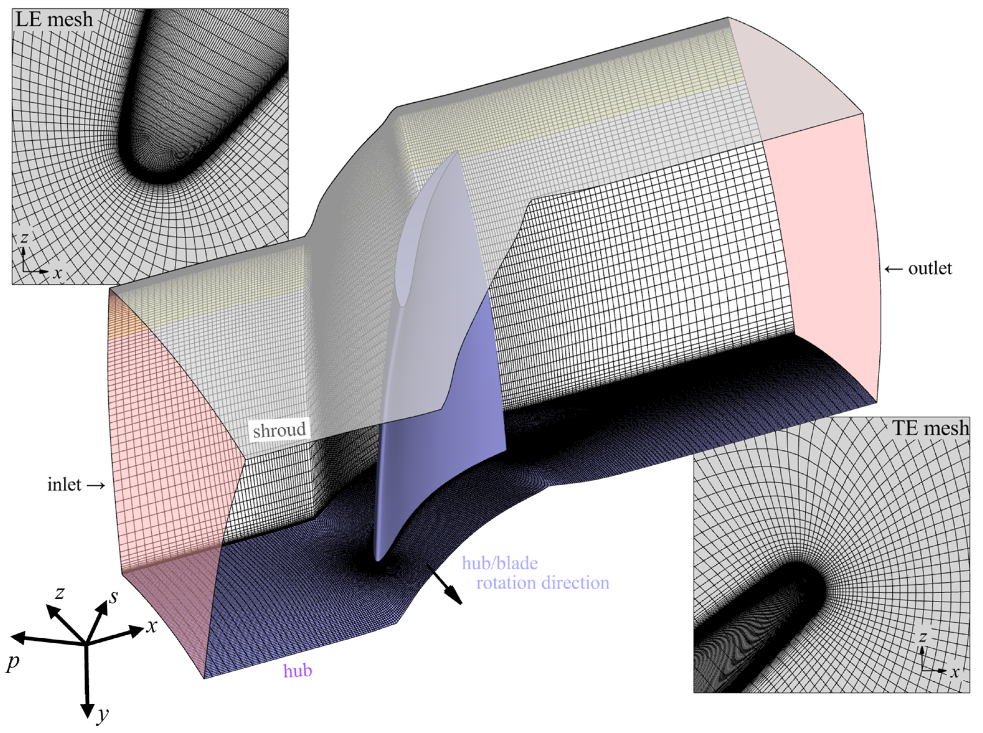
2.3. Numerical Setups

2.3.1. Experimental Configurations

Du et al. [44] conducted experimental research in the low-speed, large-scale axial compressor test rig at Beihang University. This compressor features a 1.5-stage layout that includes an inlet guide vane, a rotor, and a stator. Calculations of the Reynolds number, which were based on the length of the rotor’s tip chord (C), yielded a value of 750,000. The specific parameters of the compressor are detailed in Table 1. Velocity measurements in great detail were obtained at cross-sections that were almost perpendicular to the direction of the rotor’s tip chordwise, utilizing intervals of either 5% or 10% of the chord length through the stereoscopic particle image velocimetry (SPIV) technique. For further information on the experiment, refer to ref. [44].

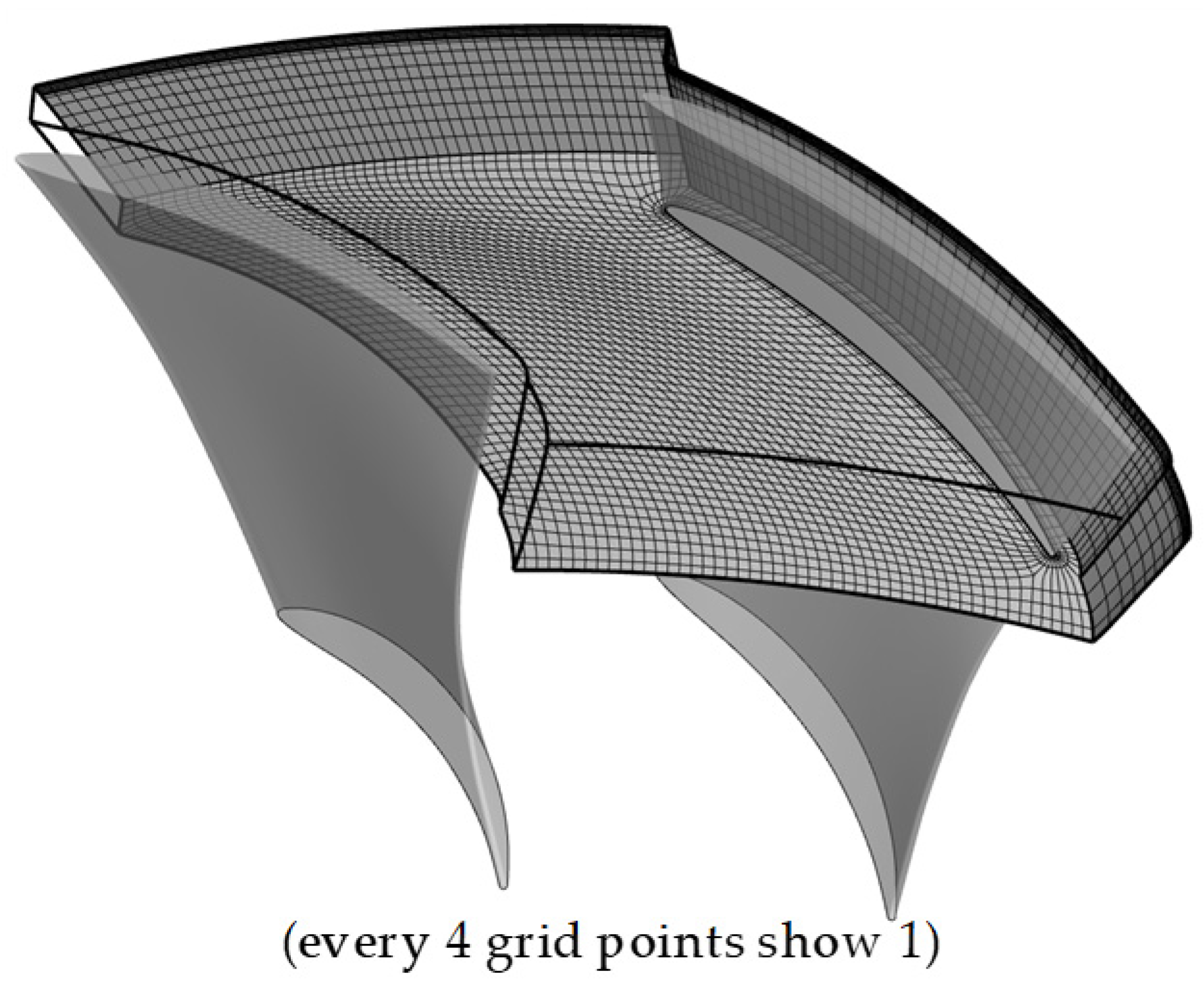
2.3.2. Computational Domain and Numerical Method

With the rapid development of computer resources, the computational fluid dynamics (CFD) technique was rapidly developed and has been widely used to study aerodynamic and aeroelastic problems [45,46]. The choice of the turbulence model plays a pivotal role in the Reynolds-averaged Navier–Stokes equations (RANS) method within engineering fields [47], and it represents a notable challenge in the aerodynamics of compressors [48], particularly concerning the analysis of tip leakage flows [49]. Hence, to explore the evolution of tip leakage flow in the rotor, the DDES method, a hybrid approach combining large eddy simulation (LES) and RANS, is utilized in this study to reduce the need for an extensive computational grid that an LES commonly requires. Compared to the RANS method, the DDES method performs significantly better in predicting the TLF [50]. This study employs the DDES method based on the shear stress transport (SST) k-ω model [51], a turbulent model that is frequently used in turbomachinery simulations [52].
For the simulation focusing on tip leakage flow, the study opted for an O4H-type mesh configuration to maintain high grid quality, as illustrated in Figure 1. The y+ is set to around 0.8 of the solid walls. The simulation’s inlet was positioned at 1.0 chord length ahead of the blade’s leading edge, with the entire computational domain extending approximately 4.0 chord lengths in the axial direction downstream. Within the TLV region, at a spanwise height exceeding 80% of the blade, refined meshes were utilized. The mesh has an aspect ratio below 2 and an expansion ratio under 1.05 to enhance the resolution of the TLV structure. The grid spacings in the spanwise, pitchwise, and streamwise dimensions relative to the blade tip’s chord length are capped at Δx+ ≤ 110, Δy+ ≤ 1, and Δz+ ≤ 120, respectively. This grid quality aligns with that of prior studies conducted under comparable flow conditions that also employed the DDES method [53,54]. The total number of grid points used in the simulation is around 6.2 million.
The simulations were performed in Fluent with a pressure-based implicit solver. The SIMPLE algorithm, an algorithm for coupling pressure and velocity, was applied in the simulations. The spatial aspect of the simulation utilized a bounded central differencing scheme for integration, while temporal discretization was achieved through second-order implicit time integration. To capture the steady total pressure distribution of the inlet flow between the inlet guide vane and the rotor, five-hole probes were strategically placed in the center of the blade passage, and the results of pressure measurements at various radii were applied to the inlet boundary condition.
In the DDES calculations, approximately 1000 time steps (Δt) cover the duration it takes for a rotor blade to pass one pitch. This time step size is selected to adequately capture the dynamics of the unsteady tip leakage flow, ensuring compliance with the Courant–Friedrichs–Lewy condition for numerical stability. The chosen time step is nondimensional, normalized by both the rotor-tip chord length and the speed of the inlet’s main flow, set at 5 × 10⁻⁴. During each time step, 30 inner iterations are executed to ensure accuracy and convergence. To comprehensively document the flow’s behavior over time, 3000 instantaneous results are recorded throughout the simulation, with a saving interval of every 10 physical time steps, providing a detailed temporal resolution of the flow characteristics.

2.3.3. Validation of the Numerical Method

The simulation results of time-averaged streamwise vorticity of the representative cross-sections at design (DE) and near-stall (NS) conditions are compared with an experimental measurement in Figure 2. To better capture the TLV, the s-y-p coordinate system is set up by rotating the x-axis and z-axis about the y-axis to the position that the x-axis is parallel to the blade tip chord and perpendicular to the cross-sections in the SPIV measurements, as shown in Figure 1. The rotated x-axis direction is termed streamwise, and the rotated z-axis direction is termed pitchwise in the following sections. The flow coefficient has been checked to guarantee that the operating point is compatible with the experiment. The flow coefficients in the simulations are 0.58 with the DE condition and 0.51 with the NS condition, respectively, showing that the agreement between them is quite good. The DDES captures the location and track of TLV at different working conditions. The simulation results capture the location of TLV and show qualitatively good agreement with experimental results.

3. Results and Discussion

3.1. Effect of Parameters on the LCS Structure in the Low-Speed Rotor

As understood from the calculation process of the FTLE, there are several parameters which affect the results of the LCSs. Three of them are considered to be the main factors, namely the initial grid of the particle trajectory, the trajectory integration method, and the integration time T. In this section, these three factors are discussed separately.

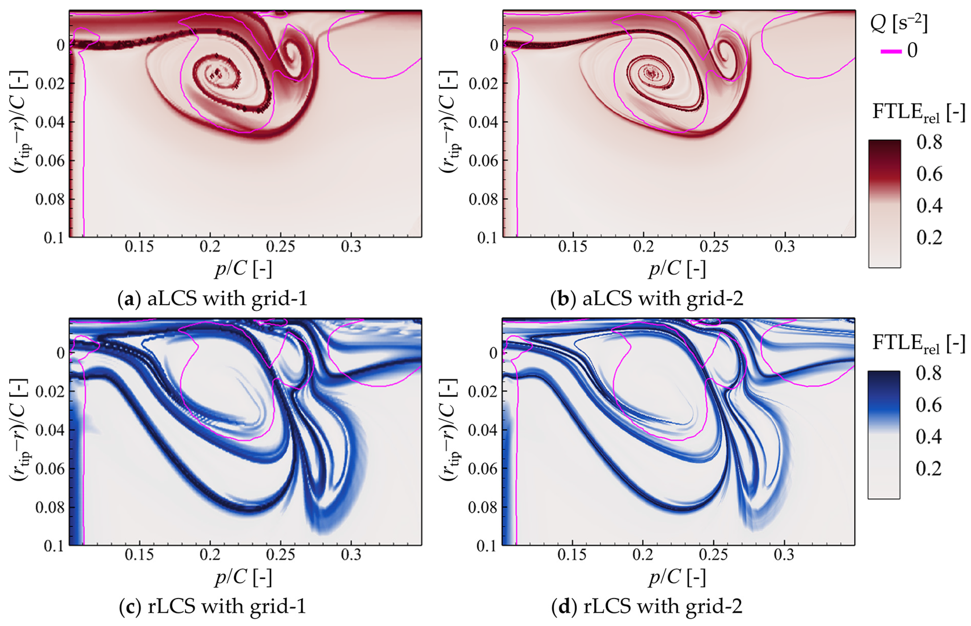
3.1.1. The Initial Grid of the Particle Trajectory

Two regular grids are compared, and the calculation parameters of the FTLE field are shown in Table 2. The initial grids are located at the cross-section of s/C = 0.5 and cover the TLV in the time-averaged flow field at DE condition. In the streamwise cross-section plane, the grid is uniform, and two layers of the grid are set in the streamwise direction to compute the derivative along this direction. The grid cells are nearly cubic. The grid of particle trajectory is advected in time as the flow field is steady. The total number of grid points in grid-2 is 6.25 times greater than that in grid-1, attributed to a 2.5-fold increase in the grid point number of grid-1 in each spatial direction. Calculations for both negative and positive integration times are performed, which correspond to aLCSs and rLCSs, respectively. The results are shown in Figure 3.
The general LCSs are similar in both grids, while the ridges are more evident in the higher-density grid. The LCSs are defined as the ‘ridges’ of the FTLE field represented by the position of local maximum values, and the exact values are not that important in illustrating the structures. For the aLCSs of the TLV core region, where the curvature of the ridge is much larger and more complicated in a small region, the differences are more significant between the two grids. For the FTLE field of forward time, the ridges are more complicated, and the lower-density initial grid mashes the ridges close to each other, forming into one.
The increasing initial grid points result in more distinct LCSs and higher computation costs simultaneously. Adaptive meshes are generated based on the FTLE fields from grid-1 to balance the calculation accuracy and costs. Regular grid points of four different densities are used to seed at different regions with various FTLE ranges and are particularly refined inside the TLV core, as shown in Table 3. Then, these seeding points are triangulated into the unstructured grid. As the grid density near the ridges stays nondecreasing, the grid numbers of the adaptive grids reduce to 27.5% and 82.7% of the grid-2 for the FTLE field of negative and positive integration time, respectively. The sketch of the adaptive grids and contours of the FTLE fields are shown in Figure 4. With the adaptive grids, the ridges are further clarified, while the general LCSs stay the same. In the core region of the TLV, where the radius of curvature of the ridges is small, the detailed aLCSs are captured with the higher-density grid. For the rLCSs, the decrement of the total grid points of the initial grid is not significant, as the structures are complicated.
For the calculation of the three-dimensional FTLE field, the cost increases sharply. To capture the LCS as that at the 2D plane, the grid number of the initial particle trajectory grid would be greatly larger than the mesh of the numerical simulation. To save computation resources, the initial grid of particle trajectory is limited to the region inside the blade row within a 25% span near the shroud. The sketch of the initial grid is shown in Figure 5, and the grid is referred to as grid-3D in this study. The total grid number of grid-3D is approximately 4.34 million.
Figure 6 shows the FTLE field and vorticity field of the time-averaged flow field with the DE condition. The Eulerian Q criterion is applied as well, and the isolines of Q = 0 s−2 are shown in Figure 6c, along with the vorticity field. Compared to the LCSs calculated from grid-1, the outlines of the general structures at the cross-section plane s/C = 0.5 are similar, while the ridges of grid-3d are rougher due to the lower density of the initial grid of the particle trajectory.
A regular grid, termed grid-3Duni, is generated and shown in Figure 7a. The total number of grid points is approximately 8.80 million, and the distributions of the grid points in each direction are uniform. The spanwise range of the grid is narrowed down to a 7.5% span to capture the TLV core and save the computational resources. The grid density at the cross-section plane s/C = 0.5 is nearly half of grid-1.
This grid gets clearer ridge structures of the FTLE field than the other 3D grid, especially with the high curvature. However, compared with the results from grid-1, the detailed LCSs cannot be distinguished, while the computational costs are far beyond that of grid-1. Limited by computational resources and efficiency, the identification of LCSs in 3D presents the overall LCSs in the whole flow field, and detailed LCSs are more suitable for identification in 2D.

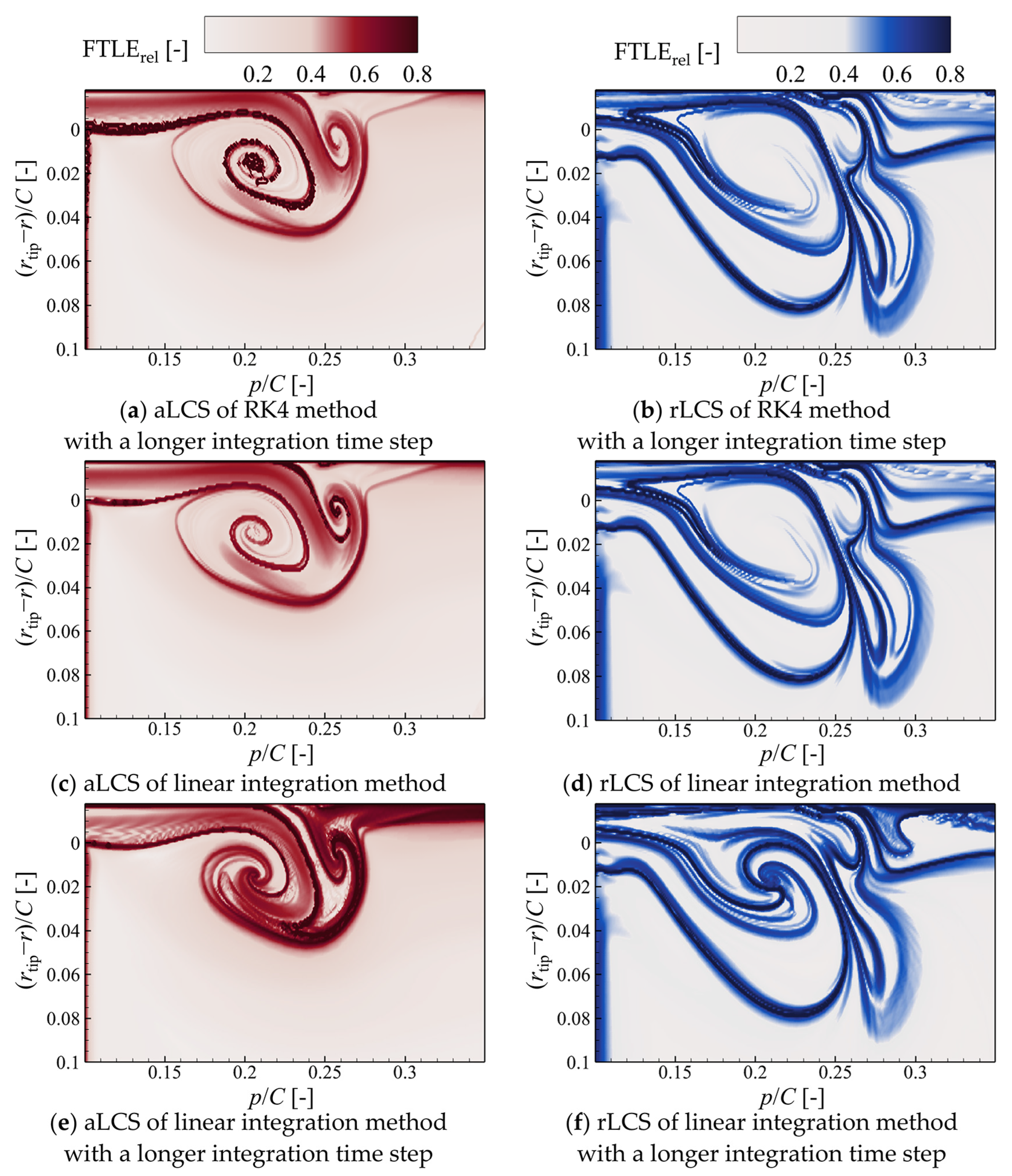
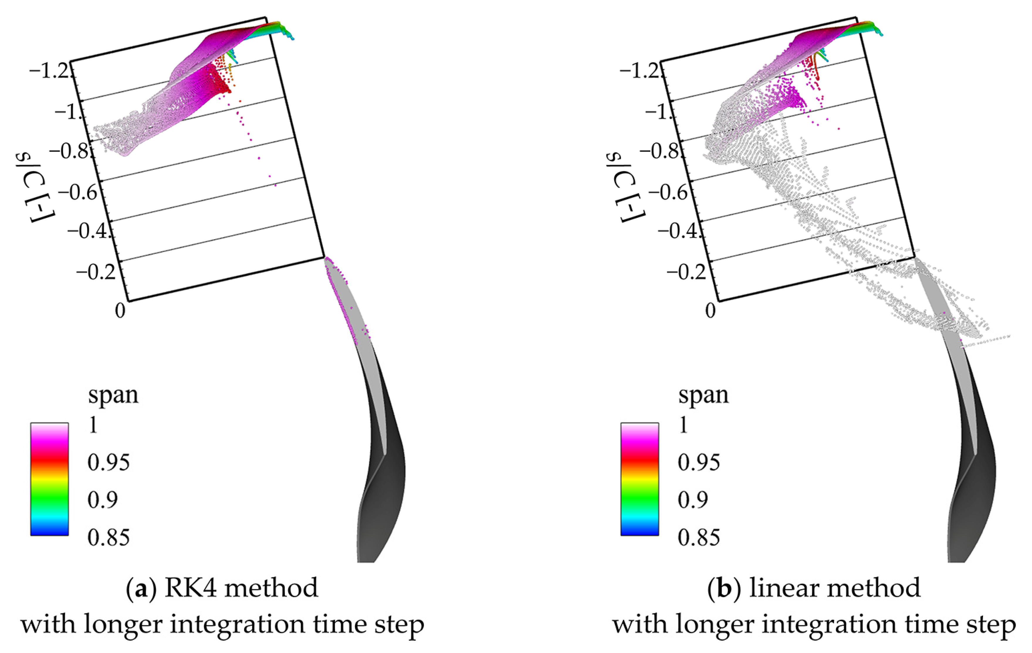
3.1.2. The Time Integration Method

The time integrations of all the particle trajectories results above are carried out by the fourth-order Runge–Kutta method. To test the effect of the time integration method, the time integrations are performed via the fourth-order Runge–Kutta method, with a longer integration time step, and the linear integration method with two integration time steps; the FTLE fields are shown in Figure 8. The impact of the time integration method falls primarily in the aLCSs, while the rLCSs are almost unaffected. Compared to the aLCSs in Figure 3c, the ridges of the TLV become rougher with the longer time step, while the general shape and scale of the ridges stay the same. The ridges of the induced vortex stand out when using the low-order time integration method. The ridges of both the TLV and the induced vortex shrink towards the core, and the scales of these LCSs are all reduced. The results are more sensitive to the integration time step length when using the linear method. When increasing the integration time step length from 2.5 Δt to the longer integration time step of 20 Δt, the LCSs are significantly different from the other results.
Figure 9 shows the final streamwise position of the particle with different time integration methods. When applying the time integration in a negative time direction, the ridges of the TLV and IV are related to two regions of large particle separations, respectively, with one being near the shear layer at the blade tip, while the other is near the shear layer at the shroud. For an axial rotor, the blade is relatively thin, and the clearance is small. However, the flow inside the gap is complex, featuring vortex structures and jet flows. When particles advect to the gap, a large time interval may lead them to pass the gap within a few integration steps, and thus, it is difficult to capture the flow features inside the gap. The RK4 method performs better than the linear method in tracking the particles inside the gap and thus gives a more stable structure of the LCSs.
Figure 10 shows the 3D view of the final position of the particles with different time integration methods with an integration time step of 20 Δt. The differences in the final positions of the particles between the two methods mainly exist in the particles that have passed the blade gap. For the linear method, a great part of the particles is finally located near the shroud. The particles near the shroud tend to be trapped in the shear layer at low speed or hit the shroud and stop. With a longer time step length, the particle trajectories further deviate with time-advecting, and the general LCSs are altered.

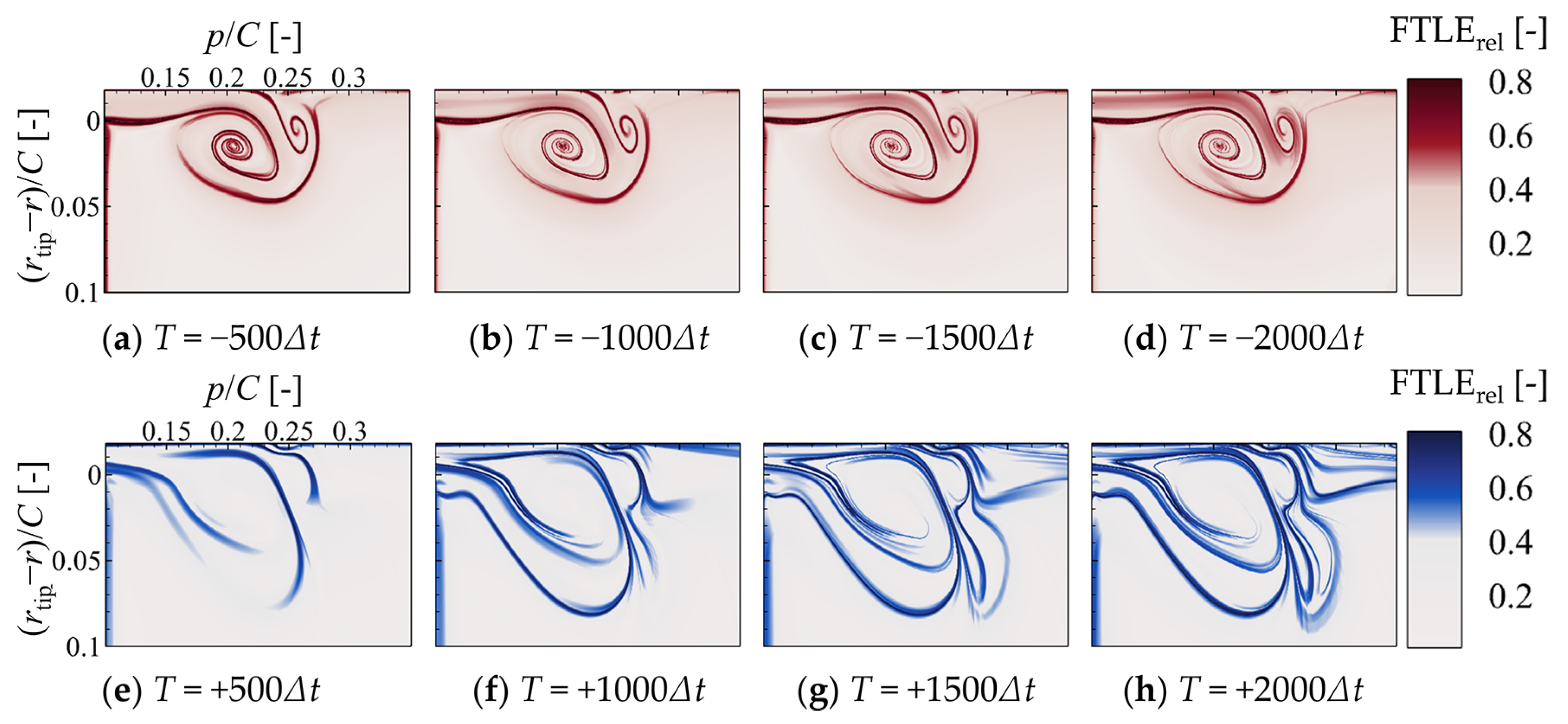
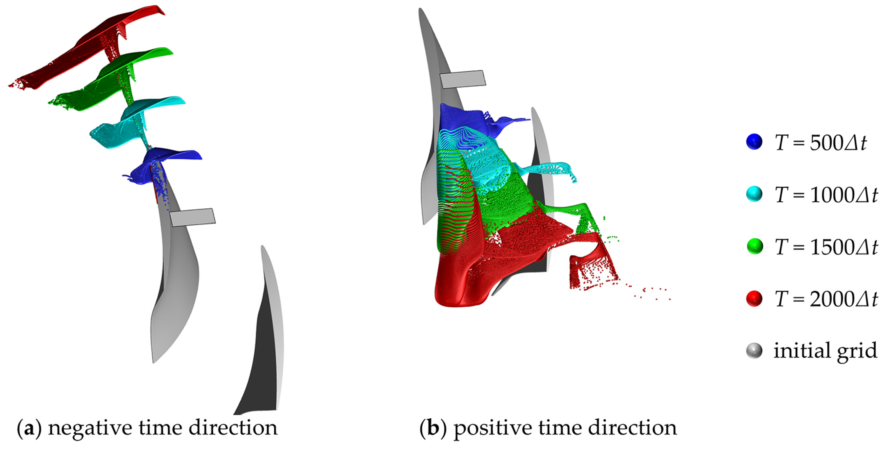
3.1.3. The Integration Time

The integration time (T) is another critical factor for the LCSs, as it determines the final position of the particle. The LCSs of a series of integration times for both negative and positive time directions are shown in Figure 11, and the corresponding final particle positions are shown in Figure 12. For the negative time direction, the particles transport ahead of the blade row where the flow is relatively undisturbed, and the general structures of the aLCSs are similar. In the positive time integration direction, the particles are transported downstream and entrained into different vortex structures, or even into the gap of the adjacent blade. Thus, more rLCSs emerge with the increase in the integration time. In this rotor, the period of a rotor blade passing through one pitch is about 1000 Δt, and the period of a particle passing through the blade row is about 1500 Δt. As the integration time length exceeds 1000 Δt, the primary LCSs tend toward stability.

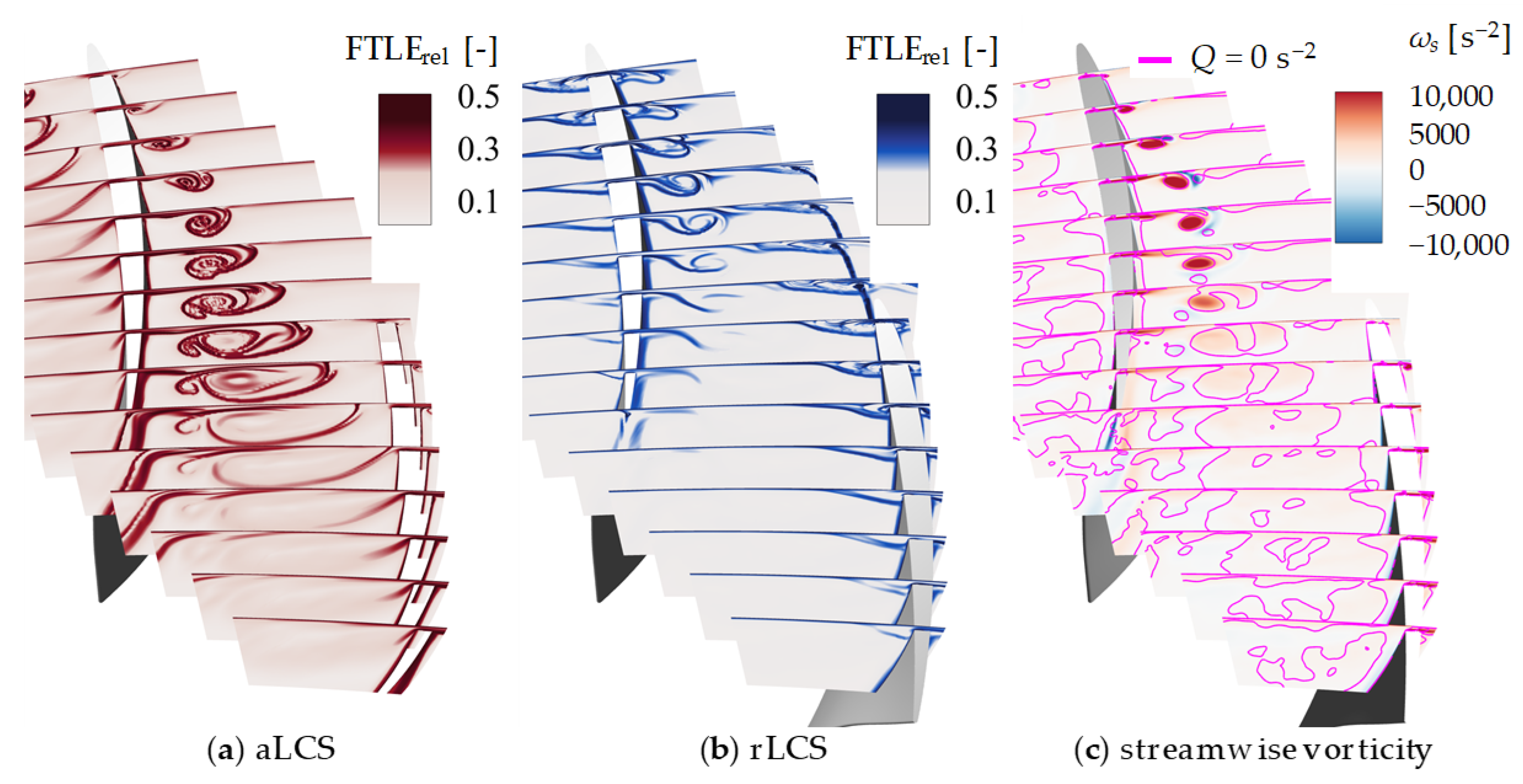
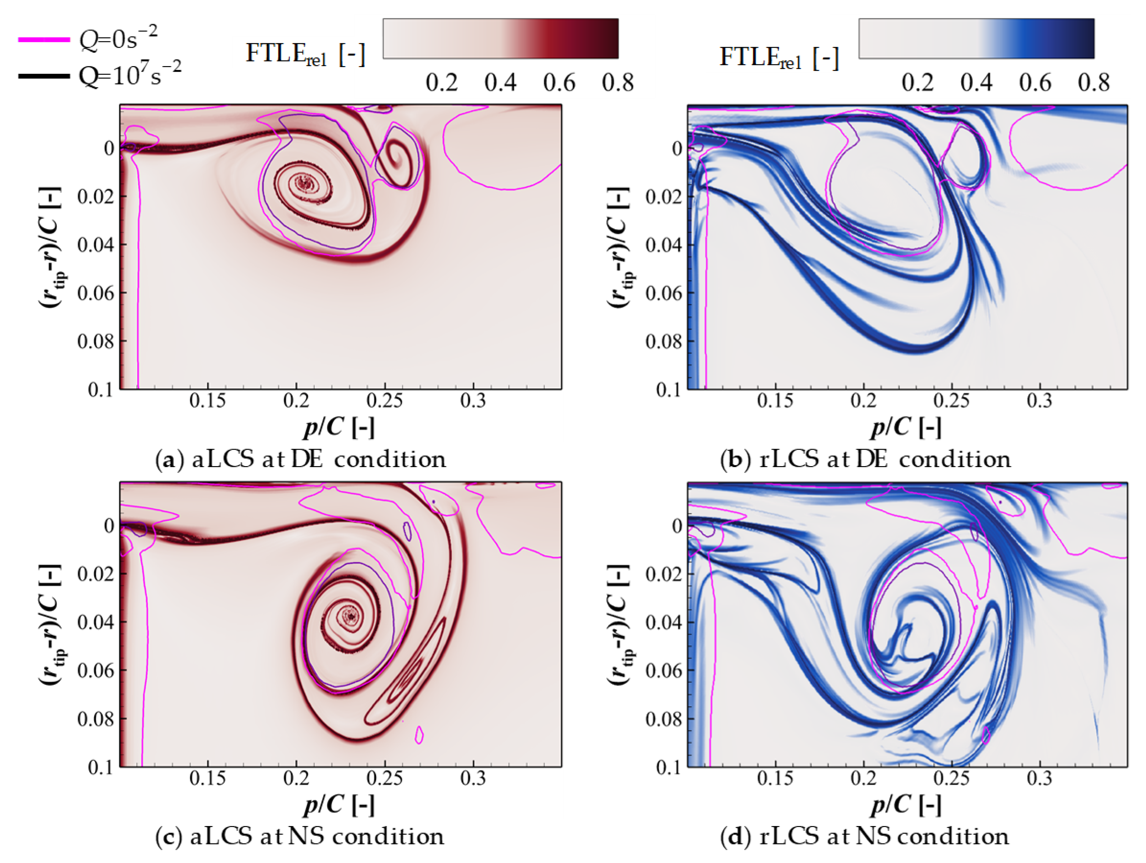
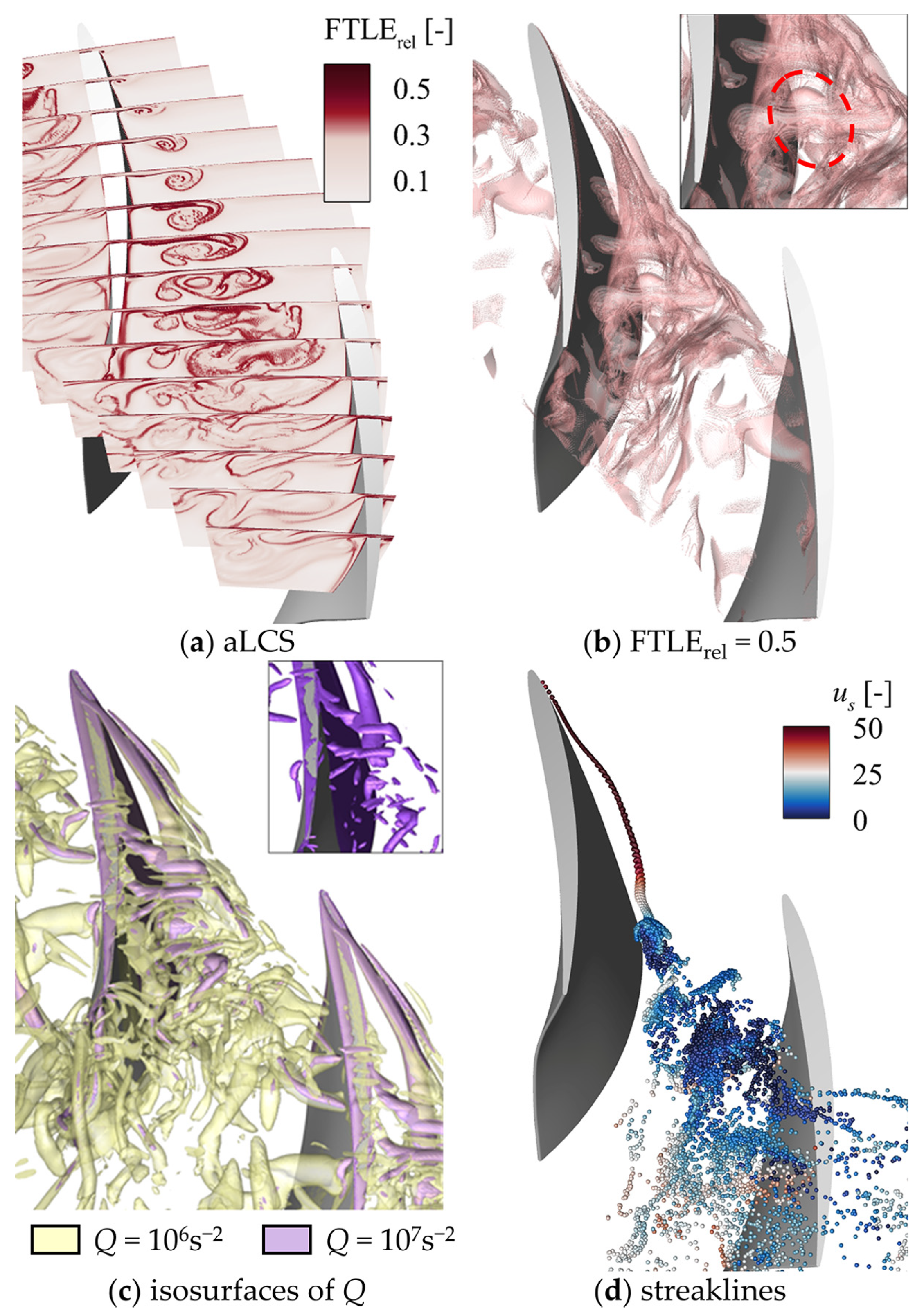
3.2. LCSs of TLF in the Low-Speed Rotor

The FTLE and vorticity fields of the time-averaged flow fields in the DE and NS conditions are shown in Figure 6 and Figure 13, respectively. The Eulerian Q criterion is applied, and the isolines of Q = 0 s−2 are shown in Figure 6c and Figure 13c, along with the vorticity field. For the time-averaged flow field, the aLCSs are similar to the TLV structure identified by the Q criterion, while the correlativity between the rLCS and the vortex structures seems weak. The region enclosed by the aLCS and the rLCS covers the TLV. In our previous study [55,56], the evolution of the TLV was divided into three phases, namely the generation phase, the development phase, and the dissipation phase. In the first two phases, the LCSs are clear, while, as the flow travels downstream, the TLV steps into the dissipation phase. In the first stage of the dissipation phase, the TLF jet shears across the passage flow and rolls up together as the secondary TLV (STLV). This structure can be confirmed by the aLCS, as clear ridges between the TLV and the STLV indicate two separate vortex structures. Then, the TLV breaks down. For the Eulerian Q criterion, the vortex structures it identified become unrecognizable. Meanwhile, for the LCSs, the aLCS gives the boundary of the passage flow entrainment.
Figure 14 shows the LCSs at the cross-section s/C = 0.5 of two instantaneous flow fields at the DE and NS conditions. The FTLE field is calculated using the grid-2, same as that in Figure 3b,d, employing the RK4 method for time integration with a step length of 2.5 Δt and a total integration period of 1000 Δt. The figure also depicts isolines for Q = 0 s−2 and 107s−2. Affected by the unsteadiness, the rLCS with the DE condition in the instantaneous flow field demonstrate a higher number of ridges than that in the steady flow field, which indicates the unstableness of the flow. With the NS condition, the TLV evolves more rapidly with higher unsteadiness, and the rLCSs exhibit increased complexity. The general structures of the aLCSs maintain consistency at the DE and NS conditions. In the DE condition, the vortex region, as identified by the Q criterion, covers the helical ridges of the TLV and induced vortex, while, with the NS condition, the vortex region identified by the Q criterion only covers the helical ridges of the TLV, especially for the higher-value regions. Part of the region at the shear layer of the TLF and passage flow is recognized as the vortex. The transport of the induced vortex is delineated by the aLCS, which is not captured by the Eulerian method.
The 3D LCSs of two instantaneous flow fields with the DE and NS conditions are shown in Figure 15 and Figure 16, respectively. The aLCSs at different streamwise cross-sections are shown in (a), the aLCS isosurfaces of FTLErel are shown in (b), the isosurfaces of Q are shown in (c), and the snapshots of the streaklines releasing along the TLV core are shown in (d) for both working conditions. A streakline is formed by continuously releasing fluid particles at a fixed point and observing the trajectories that the fluid particles reach over time. In this study, the streaklines are constructed by releasing particles along the TLV core at continuous time intervals of 10 Δt. The particle release begins from the initial sampled flow field, with particles advecting downstream with an integration time step of 10 Δt using the RK4 time integration method. The integration method is consistent with the LCS calculations. Compared to the aLCS in the time-averaged flow field, the differences are caused by the unsteadiness of the flow. The breakdown of the TLV features a characteristic unsteady flow structure in this rotor, and the breakdown patterns are different in the DE and NS conditions. Only the spiral breakdown pattern of the TLV exits at the DE condition, while the spiral and bubble breakdown patterns of the TLV appear alternately at the NS condition.
As shown in Figure 15c and Figure 16c, it is hard to assess the breakdown pattern by the isosurfaces of Q. From the snapshots of the streaklines, the breakdown patterns of these two flow fields could be distinguished: a spiral breakdown pattern for the DE condition and a bubble breakdown pattern for the NS condition. This method is commonly used to determine the breakdown pattern of vortices in the flow of pipes or delta wings. In the flow field of a rotor where the secondary flow is strong, the structure of the vortex breakdown alters, and the performance of this method relies on the judgment of the researchers. An accurate depiction of the breakdown pattern is contingent upon the strategic placement of the initial seeding points. When reducing the number of seeding points along the core, or displacing the seeding points away from the TLV core, it is hard for the streaklines to construct a bubble, and the breakdown pattern becomes ambiguous. Moreover, due to the complexity of the vortex structures, streaklines are inadequate for illustrating the features of the entire flow field, resulting in particles dispersing throughout. The isosurfaces of the aLCSs show different structures in vortex breakdown patterns. For the TLV of the bubble breakdown pattern, the surface of the TLV core ends, and a bubble-like surface appears downstream. For the TLV of the spiral breakdown pattern, the surface of the TLV core ends, and a bar-like surface appears downstream. The FTLE fields of other instantaneous flow fields have been checked for both working conditions. The aLCS patterns of each breakdown pattern correspond with the above descriptions and so are not shown here.

4. Conclusions

A Lagrangian analysis is introduced to study the LCSs of the TLF in a low-speed axial compressor rotor based on DDESs. The calculation method of the FTLE field in a 3D flow field is discussed, emphasizing three primary factors. Then, the Lagrangian method is compared with the Eulerian Q method in analyzing the vortex structures of the TLF. The main findings are summarized as follows:
(1)
The accuracy of calculating the particle advecting trajectory affects the results of the FTLE field the most. A shorter integration step or higher-order integration method would improve this accuracy.
(2)
The clarity of the ridges depends on the density of the initial grid near them. With the complex flow field as the low-speed axial compressor rotor, it is suggested that the general LCSs be detected on the coarse 3D initial grid while a two-layer mesh is then used to capture detailed LCSs.
(3)
The LCSs have advantages in identifying the relationships and interactions between vortex structures. The LCSs show a transport barrier between the TLV and the secondary TLV, indicating two separate vortices.
(4)
The breakdown patterns of the vortices in the whole flow field can be recognized clearly by the LCSs, which is not true with the Q criterion method, while the streaklines rely on subjective judgment. The aLCSs show the bubble-like and bar-like structure in the isosurfaces corresponding to the bubble and spiral breakdown patterns. The Lagrangian method has great potential in regard to unraveling the mechanism of complex vortex structures and is worth applying more in turbomachinery.

Author Contributions

Conceptualization, J.H., Y.L. and Y.T.; software, J.H.; formal analysis, J.H. and Y.T.; resources, Y.L.; data curation, J.H.; writing—original draft preparation, J.H.; writing—review and editing, Y.L. and Y.T.; visualization, J.H.; supervision, Y.L.; funding acquisition, Y.L. All authors have read and agreed to the published version of the manuscript.

Funding

This work was supported by the National Natural Science Foundation of China (Nos. 52106039, 51976006), the Industry–University–Research Cooperation Project of AECC (Grant Nos.HFZL2022CXY001 and HFZL2023CXY002), and the Fundamental Research Funds for the Central Universities.

Data Availability Statement

Data are contained within the article.

Conflicts of Interest

The authors declare no conflicts of interest.

Nomenclature

ΔtPhysical time step of simulation
tTime of instantaneous flow field
s,pStreamwise and pitchwise coordinate
CBlade tip chord length
QSecond invariant of the velocity gradient tensor
TIntegration time
uVelocity
ωVorticity
σ t 0 t 0 + T (x0)Finite-time Lyapunov exponent
FTLErelRelative finite-time Lyapunov exponent
TLVTip leakage vortex
TLFTip leakage flow
FTLEFinite-time Lyapunov exponent
aLCSAttracting Lagrangian coherent structure
rLCSRepelling Lagrangian coherent structure
DDESDelayed detached-eddy simulation
DEDesign condition
NSNear-stall condition

References

  1. Lakshminarayana, B.; Pouagare, M.; Davino, R. Three-dimensional Flow Field in the Tip Region of a Compressor Rotor Passage-Part I: Mean Velocity Profiles and Annulus Wall Boundary Layer. ASME J. Eng. Power 1982, 104, 760–772. [Google Scholar] [CrossRef]
  2. Lakshminarayana, B.; Pouagare, M.; Davino, R. Three-dimensional Flow Field in the Tip Region of a Compressor Rotor Passage-Part II: Turbulence Properties. J. Eng. Power 1982, 104, 772–781. [Google Scholar] [CrossRef]
  3. Furukawa, M.; Inoue, K.; Saiki, K.; Yamada, K. The Role of Tip Leakage Vortex Breakdown in Compressor Rotor Aerodynamics. ASME J. Turbomach. 1999, 121, 469–480. [Google Scholar] [CrossRef]
  4. Denton, J.D. Loss Mechanisms in Turbomachines. ASME J. Turbomach. 1993, 115, 621–656. [Google Scholar] [CrossRef]
  5. Kameier, F.; Neise, W. Experimental Study of Tip Clearance Losses and Noise in Axial Turbomachines and Their Reduction. ASME J. Turbomach. 1997, 119, 460–471. [Google Scholar] [CrossRef]
  6. Day, I.J. Stall, Surge, and 75 Years of Research. ASME J. Turbomach. 2016, 138, 011001. [Google Scholar] [CrossRef]
  7. Cao, Z.; Zhang, X.; Liang, Y.; Liu, B. Influence of Blade Lean on Performance and Shock Wave/Tip Leakage Flow Interaction in a Transonic Compressor Rotor. J. Appl. Fluid Mech. 2022, 15, 153–167. [Google Scholar] [CrossRef]
  8. Lu, H.; Yang, Y.; Guo, S.; Huang, Y.; Wang, H.; Zhong, J. Flow Control in Linear Compressor Cascades by Inclusion of Suction Side Dimples at Varying Locations. Proc. Inst. Mech. Eng. Part A J. Power Energy 2018, 232, 706–721. [Google Scholar] [CrossRef]
  9. Zhong, F.; Zhou, C. Effects of Tip Gap Size on the Aerodynamic Performance of a Cavity-Winglet Tip in a Turbine Cascade. ASME J. Turbomach. 2017, 139, 101009. [Google Scholar] [CrossRef]
  10. Green, M.; Rowley, C.; Haller, G. Detection of Lagrangian Coherent Structures in 3D Turbulence. J. Fluid Mech. 2007, 572, 111–120. [Google Scholar] [CrossRef]
  11. Helmholtz, H. On the Integrals of the Hydrodynamic Equations Corresponding to Vortex Motions. Lond. Edinb. Dublin Philos. Mag. J. Sci. 1867, 33, 485–512. [Google Scholar] [CrossRef]
  12. Hunt, J.C.; Wray, A.A.; Moin, P. Eddies, Streams, and Convergence Zones in Turbulent Flows. Cent. Turbul. Res. Rep. 1988, CTR-S88, 193–208. [Google Scholar]
  13. Duda, D.; Yanovych, V.; Uruba, V. Vortex Profiles in Grid Turbulence Observed by PIV. AIP Conf. Proc. 2023, 2672, 020002. [Google Scholar] [CrossRef]
  14. Chong, M.S.; Perry, A.E.; Cantwell, B.J. A General Classification of Three-Dimensional Flow Fields. Phys. Fluids 1990, 2, 765–777. [Google Scholar] [CrossRef]
  15. Jeong, J.; Hussain, F. On the Identification of a Vortex. J. Fluid Mech. 1995, 285, 69–94. [Google Scholar] [CrossRef]
  16. Liu, C.; Xu, H.; Cai, X.; Gao, Y. Liutex and Its Applications in Turbulence Research, 1st ed.; Elsevier: Amsterdam, The Netherlands, 2020; ISBN 978-012-819-023-4. [Google Scholar]
  17. Zhong, W.; Liu, Y.; Tang, Y. Unsteady Flow Structure of Corner Separation in a Highly Loaded Compressor Cascade. ASME J. Turbomach. 2024, 146, 031003. [Google Scholar] [CrossRef]
  18. Hou, J.; Liu, Y. Effect of Moving End Wall on Tip Leakage Flow in a Compressor Cascade with Different Clearance Heights. AIP Adv. 2024, 14, 015327. [Google Scholar] [CrossRef]
  19. Haller, G.; Yuan, G. Lagrangian Coherent Structures and Mixing in Two-Dimensional Turbulence. Phys. D 2000, 147, 352–370. [Google Scholar] [CrossRef]
  20. D’Ovidio, F.; Fernández, V.; Hernández-García, E.; López, C. Mixing Structures in the Mediterranean Sea from Finite-Size Lyapunov Exponents. Geophys. Res. Lett. 2004, 31, L17203. [Google Scholar] [CrossRef]
  21. Prants, S. Transport Barriers in Geophysical Flows: A Review. Symmetry 2023, 15, 1942. [Google Scholar] [CrossRef]
  22. Lekien, F.; Coulliette, C.; Mariano, A.J.; Ryan, E.H.; Shay, L.K.; Haller, G.; Marsden, J. Pollution Release Tied to Invariant Manifolds: A Case Study for The Coast of Florida. Physica D 2005, 210, 1–20. [Google Scholar] [CrossRef]
  23. Sapsis, T.; Haller, G. Inertial Particle Dynamics in a Hurricane. J. Atmos. Sci. 2009, 66, 2481–2492. [Google Scholar] [CrossRef]
  24. Shadden, S.C.; Astorino, M.; Gerbeau, J.-F. Computational Analysis of An Aortic Valve Jet with Lagrangian Coherent Structures. Chaos 2010, 20, 017512. [Google Scholar] [CrossRef] [PubMed]
  25. Shadden, S.C.; Taylor, C.A. Characterization of Coherent Structures in the Cardiovascular System. Ann. Biomed. Eng. 2008, 36, 1152–1162. [Google Scholar] [CrossRef] [PubMed]
  26. He, G.; Pan, C.; Feng, L.; Gao, Q.; Wang, J. Evolution of Lagrangian Coherent Structures in a Cylinder-Wake Disturbed Flat Plate Boundary Layer. J. Fluid Mech. 2016, 792, 274–306. [Google Scholar] [CrossRef]
  27. Pan, C.; Wang, J.; Zhang, C. Identification of Lagrangian Coherent Structures in the Turbulent Boundary Layer. Sci. China Ser. G-Phys. Mech. Astron. 2009, 52, 248–257. [Google Scholar] [CrossRef]
  28. Li, S.; Jiang, N.; Yang, S.; Huang, Y.; Wu, Y. Coherent Structures over Riblets in Turbulent Boundary Layer Studied by Combining Time-Resolved Particle Image Velocimetry (TRPIV), Proper Orthogonal Decomposition (POD), and Finite-Time Lyapunov Exponent (FTLE). Chin. Phys. B. 2018, 27, 104701. [Google Scholar] [CrossRef]
  29. Rockwood, M.P.; Taira, K.; Green, M.A. Detecting Vortex Formation and Shedding in Cylinder Wakes Using Lagrangian Coherent Structures. AIAA J. 2017, 55, 15–23. [Google Scholar] [CrossRef]
  30. Olcay, A.B. Investigation of a wake formation for flow over a cylinder using Lagrangian coherent structures. Prog. Comput. Fluid Dyn. 2016, 16, 2. [Google Scholar] [CrossRef]
  31. Wang, W.; Prants, S.V.; Zhang, J.; Zhang, J.; Wang, L. A Lagrangian Analysis of Vortex Formation in the Wake behind a Transversely Oscillating Cylinder. Regul. Chaot. Dyn. 2018, 23, 583–594. [Google Scholar] [CrossRef]
  32. Sun, P.N.; Colagrossi, A.; Marrone, S.; Zhang, A.M. Detection of Lagrangian Coherent Structures in the SPH framework. Comput. Methods Appl. Mech. Eng. 2016, 305, 849–868. [Google Scholar] [CrossRef]
  33. Wang, L.; Wang, P.; Chang, Z.; Huang, B.; Wu, D. A Lagrangian Analysis of Partial Cavitation Growth and Cavitation Control Mechanism. Phys. Fluids 2022, 34, 113329. [Google Scholar] [CrossRef]
  34. Ahmad, R.; Zhang, J.; Farooqi, A.; Nauman Aslam, M. Transport Phenomena and Mixing Induced by Vortex Formation in Flow Around Airfoil Using Lagrangian Coherent Structures. Numer. Math. Theor. Meth. Appl. 2019, 12, 1231–1245. [Google Scholar] [CrossRef]
  35. Tang, J.; Tseng, C.; Wang, N. Lagrangian-Based Investigation of Multiphase Flows by Finite-Time Lyapunov Exponents. Acta. Mech. Sin. 2012, 28, 612–624. [Google Scholar] [CrossRef]
  36. Tu, H.; Marzanek, M.; Green, M.A.; Rival, D.E. FTLE and Surface-Pressure Signature of Dynamic Flow Reattachment During Delta-Wing Axial Acceleration. AIAA J. 2022, 60, 2178–2194. [Google Scholar] [CrossRef]
  37. Li, K.; Savari, C.; Barigou, M. Computation of Lagrangian Coherent Structures from Experimental Fluid Trajectory Measurements in a Mechanically Agitated Vessel. Chem. Eng. Sci. 2022, 254, 117598. [Google Scholar] [CrossRef]
  38. Tseng, C.; Hu, H. Flow Dynamics of a Pitching Foil by Eulerian and Lagrangian Viewpoints. AIAA J. 2016, 54, 712–727. [Google Scholar] [CrossRef]
  39. Haller, G. Distinguished Material Surfaces and Coherent Structures in Three-Dimensional Fluid Flows. Phys. D 2001, 149, 248–277. [Google Scholar] [CrossRef]
  40. Shadden, S.C. A Dynamical Systems Approach to Unsteady Systems; California Institute of Technology: Pasadena, CA, USA, 2006. [Google Scholar]
  41. Haller, G.; Sapsis, T. Lagrangian Coherent Structures and the Smallest Finite-Time Lyapunov Exponent. Chaos 2011, 21, 023115. [Google Scholar] [CrossRef]
  42. Shadden, S.C.; Lekien, F.; Marsden, J.E. Definition and Properties of Lagrangian Coherent Structures from Finite-Time Lyapunov Exponents in Two-Dimensional Aperiodic Flows. Phys. D 2005, 212, 271–304. [Google Scholar] [CrossRef]
  43. Lekien, F.; Shadden, S.C.; Marsden, J.E. Lagrangian Coherent Structures in n-Dimensional Systems. J. Math. Phys. 2007, 48, 065404. [Google Scholar] [CrossRef]
  44. Du, H.; Yu, X.; Zhang, Z.; Liu, B. Relationship Between the Flow Blockage of Tip Leakage Vortex and Its Evolutionary Procedures inside the Rotor Passage of a Subsonic Axial Compressor. J. Therm. Sci. 2013, 22, 522–531. [Google Scholar] [CrossRef]
  45. Liu, Y.; Zhao, S.; Wang, F.; Tang, Y. A Novel Method for Predicting Fluid-Structure Interaction with Large Deformation Based on Masked Deep Neural Network. Phys. Fluids 2024, 36, 027103. [Google Scholar] [CrossRef]
  46. Liu, Y.; Wang, F.; Zhao, S.; Tang, Y. A Novel Framework for Predicting Active Flow Control by Combining Deep Reinforcement Learning and Masked Deep Neural Network. Phys. Fluids 2024, 36, 037112. [Google Scholar] [CrossRef]
  47. Spalart, P.R. Philosophies and Fallacies in Turbulence Modeling. Prog. Aerosp. Sci. 2015, 74, 1–15. [Google Scholar] [CrossRef]
  48. Liu, Y.; Wei, X.; Tang, Y. Investigation of Unsteady Rotor–Stator Interaction and Deterministic Correlation Analysis in a Transonic Compressor Stage. ASME J. Turbomach. 2023, 145, 071004. [Google Scholar] [CrossRef]
  49. Lee, G.H.; Park, J.I.; Baek, J.H. Performance Assessment of Turbulence Models for the Quantitative Prediction of Tip Leakage Flow in Turbomachines. In Proceedings of the ASME Turbo Expo 2004: Power for Land, Sea, and Air, Volume 5: Turbo Expo 2004, Parts A and B, Vienna, Austria, 14–17 June 2004; pp. 1501–1512. [Google Scholar] [CrossRef]
  50. Liu, Y.; Zhong, L.; Lu, L. Comparison of DDES and URANS for Unsteady Tip Leakage Flow in an Axial Compressor Rotor. ASME J. Fluids Eng. 2019, 141, 121405. [Google Scholar] [CrossRef]
  51. Gritskevich, M.S.; Garbaruk, A.V.; Schütze, J.; Menter, F.R. Development of DDES and IDDES Formulations for the k-ω Shear Stress Transport Model. Flow Turbul. Combust. 2012, 88, 431–449. [Google Scholar] [CrossRef]
  52. Menter, F.R.; Kuntz, M.; Langtry, R. Ten Years of Industrial Experience with the SST Turbulence Model. In Turbulence, Heat and Mass Transfer 4; Hanjalic, K., Nagano, Y., Tummers, M.J., Eds.; Begell House: New York, NY, USA; Wallingford, UK, 2003; Volume 4, pp. 625–632. [Google Scholar]
  53. Tucker, P. Unsteady Computational Fluid Dynamics in Aeronautics; Fluid Mechanics and Its Applications; Springer: Dordrecht, The Netherlands, 2013; Volume 104. [Google Scholar] [CrossRef]
  54. Li, H.; Su, X.; Yuan, X. Entropy Analysis of the Flat Tip Leakage Flow with Delayed Detached Eddy Simulation. Entropy 2019, 21, 21. [Google Scholar] [CrossRef]
  55. Hou, J.; Liu, Y.; Zhong, L.; Zhong, W.; Tang, Y. Effect of Vorticity Transport on Flow Structure in the Tip Region of Axial Compressors. Phys. Fluids 2022, 34, 055102. [Google Scholar] [CrossRef]
  56. Hou, J.; Liu, Y. Evolution of Unsteady Vortex Structures in the Tip Region of an Axial Compressor Rotor. Phys. Fluids 2023, 35, 045107. [Google Scholar] [CrossRef]
Figure 1. Computation domain and mesh of the rotor.
Symmetry 16 00344 g001
Figure 2. Time-averaged streamwise vorticity of different conditions. (a) Experimental result at the DE condition; (b) DDES result at the DE condition; (c) experiment result at the NS condition; (d) DDES result at the NS condition.
Symmetry 16 00344 g002
Figure 3. Sketch of initial grids and contours of an FTLE field with different regular grids. Contours of aLCS and isolines of Q = 0 s−2 with (a) grid-1 and (b) grid-2; contours of rLCS and isolines of Q = 0 s−2 with (c) grid-1 and (d) grid-2.
Symmetry 16 00344 g003
Figure 4. Sketch of adaptive grids and contours of FTLE field with different direction of integration times. (a) Sketch of adaptive grid for aLCS; (b) sketch of adaptive grid for rLCS; (c) contours of aLCS; (d) contours of rLCS.
Symmetry 16 00344 g004
Figure 5. Sketch of the initial grid grid-3D.
Symmetry 16 00344 g005
Figure 6. FTLE field and vorticity field of the time-averaged flow field at the DE condition. (a) Contours of aLCS; (b) contours of rLCS; (c) streamwise vorticity with Q = 0 s−2.
Symmetry 16 00344 g006
Figure 7. Sketch of grid-3Duni and FTLE field of time-averaged flow field at DE condition. (a) sketch of grid-3Duni; (b) contours of aLCS.
Symmetry 16 00344 g007
Figure 8. The FTLE field of different time integration methods. (a) Contours of aLCS of RK4 method with integration time step of 20 Δt; (b) contours of rLCS of RK4 method with an integration time step of 20 Δt; (c) contours of aLCS of linear integration method with an integration time step of 2.5 Δt; (d) contours of rLCS of linear integration method with an integration time step of 2.5 Δt; (e) contours of aLCS of linear integration method with an integration time step of 20 Δt; (f) contours of rLCS of linear integration method with an integration time step of 20 Δt.
Symmetry 16 00344 g008
Figure 9. Final streamwise position of the particles with different time integration methods. (a) RK4 method with an integration time step of 2.5 Δt; (b) linear method with an integration time step of 2.5 Δt; (c) RK4 method with an integration time step of 20 Δt; (d) linear method with an integration time step of 20 Δt.
Symmetry 16 00344 g009
Figure 10. Final position of the particles with different time integration methods. (a) RK4 method with an integration time step of 20 Δt; (b) linear method with an integration time step of 20 Δt.
Symmetry 16 00344 g010
Figure 11. The LCSs of a series of integration times, both negative and positive, and the time direction of the time-averaged flow field at the DE condition. (a) Integration time of T = −500 Δt; (b) integration time of T = −1000 Δt; (c) integration time of T = −1500 Δt; (d) integration time of T = −2000 Δt; (e) integration time of T = +500 Δt; (f) integration time of T = +1000 Δt; (g) integration time of T = +1500 Δt; (h) integration time of T = +2000 Δt.
Symmetry 16 00344 g011
Figure 12. Final particle positions of a series of integration times. (a) Negative time direction for aLCS; (b) positive time direction for rLCS.
Symmetry 16 00344 g012
Figure 13. TLV structure in the time-averaged flow field at the NS condition. (a) contours of aLCS; (b) contours of rLCS; (c) contours of streamwise vorticity with isonlines of Q = 0 s−2.
Symmetry 16 00344 g013
Figure 14. FTLE field with isolines of Q in the instantaneous flow field of cross-section s/C = 0.5 at t = +17,500 Δt at the DE and NS conditions. Contours of (a) aLCS and (b) rLCS with the DE condition; (c) aLCS and (d) rLCS with the NS condition.
Symmetry 16 00344 g014
Figure 15. FTLE field, Q, and streaklines of instantaneous flow field at t = +17,500 Δt at the DE condition. (a) Contours of aLCS; (b) isosurfaces of FTLErel = 0.6; (c) isosurfaces of Q; (d) snapshot of streaklines.
Symmetry 16 00344 g015
Figure 16. FTLE field, Q, and streaklines of instantaneous flow field at t = +17,500 Δt at the NS condition. (a) Contours of aLCS; (b) isosurfaces of FTLErel = 0.6; (c) isosurfaces of Q; (d) snapshot of streaklines.
Symmetry 16 00344 g016
Table 1. Design parameters of the test facility.
ParameterParameter Value
Outer diameter1.0 m
Hub-to-tip ratio0.6
Design Speed1200 r/min
ConfigurationInlet guide vane + Rotor + Stator
Number of rotor blades17
Mid-span blade chord152 mm
Mid-span Blade camber angle40.8°
Mid-span Blade stagger angle36.5°
Solidity (mid-span)1.03
Aspect ratio (mid-span)1.32
Rotor tip gap3.5 mm
Rotor tip gap/blade height1.75%
Table 2. Calculation parameters of FTLE field with different regular grids.
Grid No.Grid SizeIntegration Time StepIntegration TimeTime Integration Method
1300(p) × 180(r)2.5 Δt±2000 ΔtFourth-order Runge-Kutta
2750(p) × 450(r)2.5 Δt±2000 ΔtFourth-order Runge-Kutta
Table 3. Grid densities for different FTLE ranges.
Grid Density LevelGrid SizeFTLE Range
1150(p) × 90(r)(−∞, 0.27]
2300(p) × 180(r)(0.27, 0.56)
3750(p) × 450(r)[0.56, +∞)
41500(p) × 900(r)[0.56, +∞) (partial)
Disclaimer/Publisher’s Note: The statements, opinions and data contained in all publications are solely those of the individual author(s) and contributor(s) and not of MDPI and/or the editor(s). MDPI and/or the editor(s) disclaim responsibility for any injury to people or property resulting from any ideas, methods, instructions or products referred to in the content.

