Article

Curve-Surface Pairs on Embedded Surfaces and Involute D-Scroll of the Curve-Surface Pair in E3

by
Filiz Ertem Kaya
1,*,† and
Süleyman Şenyurt
2,†
1
Department of Mathematics, Faculty of Science and Arts, Niğde Ömer Halisdemir University, Niğde 51240, Turkey
2
Department of Mathematics, Ordu University, Ordu 52200, Turkey
*
Author to whom correspondence should be addressed.
These authors contributed equally to this work.
Symmetry 2024, 16(3), 323; https://doi.org/10.3390/sym16030323
Submission received: 22 January 2024 / Revised: 20 February 2024 / Accepted: 22 February 2024 / Published: 7 March 2024
(This article belongs to the Special Issue Symmetry/Asymmetry: Differential Geometry and Its Applications)

Abstract

:
Willmore defined embedded surfaces on f : S E 3 , which is the embedding of S into Euclidean 3-space. He investigated the Euclidean metric of E 3 , inducing a Riemannian structure on f ( S ) . The expression analogous to the left-hand member of the curvature K is replaced by the mean curvature H 2 on f ( S ) . Our aim is to observe the Gaussian and mean curvatures of curve–surface pairs using embedded surfaces in different curve–surface pairs and to define some developable operations on their curve–surface pairs. We also investigate the embedded surfaces using the Willmore method. We first recall the Darboux curve–surface and derive the new characterizations. This curve–surface pair is called the osculating Darboux curve–surface if its position vector always lies in the osculating Darboux plane spanned by a Darboux frame. Thus, we observed an osculating Darboux curve–surface pair. We also obtained the D -scroll of the curve–surface pair and involute D -scroll of the curve–surface pair with some differential geometric elements and found D ( α , M ) ( s ) and D ( α , M ) ( s ) -scrolls of the curve–surface pair ( α , M ) .

1. Introduction

Curves, surfaces, and curve–surface pairs are essential structures in differential geometry. Willmore defined embedded surfaces on f : S E 3 as embedding of S into Euclidean 3-space. He took the Euclidean metric of E 3 and induced it to a Riemannian structure on f ( S ) , considered an expression analogous to the left-hand member of the curvature K, and replaced it with the mean curvature H 2 on f ( S ) .
Similar to the work in [1], in this study, we introduce a novel concept of embedded surface with curve–surface pairs, and present fresh insights by offering new characterizations for these pairs within Euclidean 3-space. This marks the first comprehensive exploration of curve–surface pairs theory in this context, establishing both necessary and sufficient conditions.
Frenet frame geometric studies were constructed in [2,3,4,5,6,7,8]. Similar studies were conducted in [9,10,11,12,13,14,15]. For example, Chen [5] observed rectifying curves and an invariant of the rectifying curve. By using the Frenet frame, the envelope of the plane spanned is also examined in [5,13]. Moreover, Takeuchi and Izumiya [12] showed the proofs that a developable surface with a geodesic as a rectifying curve is a conical surface. There are also other papers on this subject, as seen in [16,17,18,19,20]. In addition, based on the results in [7,10,15,16], Takahashi studied the relations between the invariants of the Darboux curve and osculating Darboux curve in [19].
A regular curve is defined by curvatures κ and τ and a curve–surface pair is defined by curvatures k n , k g and t r . A regular curve is called a general helix if its first and second curvatures κ and τ are not constant, but κ τ is constant.
Many papers have considered the involute–evolute curves. for example [21,22,23]. Using a similar method, we produce a new ruled surface based on another ruled surface. In [21], D -scroll, which is known as the rectifying developable surface, of any curve α and the involute D -scroll of the curve α are already defined as E 3 . In [21,22,23], special ruled surfaces of D -scroll and involute D -scroll are considered, which are associated with a space curve α with a curvature κ 0 and involute β .
The objective of this study is to analyze the Gaussian and mean curvatures of curve–surface pairs utilizing embedded surfaces across various curve–surface pair configurations. Additionally, we aim to perform developable operations on these curve–surface pairs, thoroughly investigating their properties. We employ the Gauss–Bonnet theorem by Willmore to characterize developable curve–surface pairs, particularly focusing on those whose position vectors align with the planes spanned by the osculating Darboux frame, as discussed in [1]. Also, we obtain the D -scroll within a specific type of strip and the involute D -scroll within another type of strip, incorporating various differential geometric components such as the Weingarten map S, mean, and Gaussian curvatures. Notably, we explore the curvatures of the a , b , c invariants, denoted as k n = b , k g = c , t r = a (Curvatures of a Strip) and determine D ( α , M ) ( s ) and D ( α , M ) ( s ) s c r o l l s of the strip ( α , M ) along with the modified Darboux vector field of the involute ( β , M ) , following methodologies outlined in previous works [1,7,16,21,22,23].
Then, we review some basic concepts regarding curve–surface pairs, embedded surfaces, osculating Darboux frame, and D -scroll with some differential geometric elements.

2. Preliminaries

Definition 1. 
Let α : I R 3 be a curve α ´ ( s ) 0 where T ( s ) = α ´ ( s ) is a unit tangent vector of α at s and M is a surface in Euclidean 3-space. We define a surface element of M as the part of a tangent plane at the neighbour of the point. The locus of the these surface elements along the curve is called a curve–surface pair, shown as ( α , M ) , [24].
Definition 2. 
Let t be the tangent vector field of curve α, n be the normal vector field of the curve α, and b be the binormal vector field of curve α [17]. Frenet vectors of the curve are shown as V 1 , V 2 , V 3 . Here, V 1 = t , V 2 = n , V 3 = b . The strip vector fields of a strip that belong to curve α are ξ , η , ζ . These vector fields are:
Strip tangent vector field is t = ξ
Strip normal vector field is ζ = N
Strip binormal vector field is η = ζ Λ ξ ([17]).
We can write
t = ξ n = cos φ η + sin φ ζ b = sin φ η + cos φ ζ .
Let t , n , b and ξ , η , ζ be the curve and the curve–surface pair’s vector fields. The curve–surface pair tangent vector field, normal vector field, and binormal vector field are provided by t = ξ , ζ = N and η = ξ ζ . Curve α has two curvatures, κ and τ . A curve has a curve–surface pair with three curvatures k n = b , k g = c , t r = a , which are the normal curvature, geodesic curvature, and geodesic torsion of the curve–surface pair. If ξ , η , ζ is the curve–surface pair’s vector fields on α , we have derivatives of the ξ , η , ζ ,
ξ ´ = c η b ζ η ´ = c ξ + a ζ ζ ´ = b ξ a η .
Let φ be the angle between b and ζ . From the last equation we have ξ   ´ = c η b ζ . If we substitute ξ = t in last equation, we obtain
ξ   ´ = κ n
and
b = κ sin φ , c = κ cos φ
From the last two equations, we obtain,
κ 2 = b 2 + c 2
which denotes the relationship between the curvature κ of a curve α and the normal curvature and the geodesic curvature of a curve–surface pair [17].
By using similar operations, we obtain a new equation, as follows
τ = a + b ´ c b c ´ b 2 + c 2
which shows the relationship between τ (torsion or second curvature of α ) and a , b , c curvatures of a curve–surface pair that belongs to the curve α . From [17] we can also write
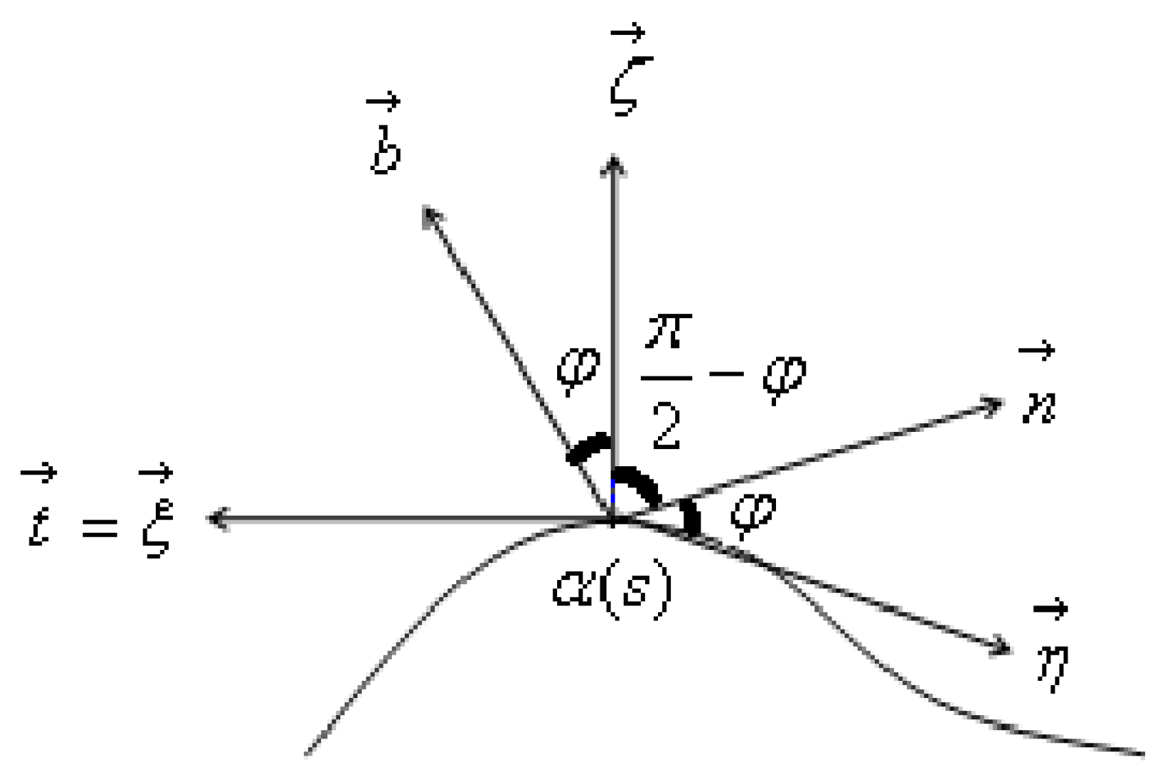
a = φ   ´ + τ .
Definition 3. 
Let α be a curve in M E 3 . If the geodesic curvature (torsion) of curve α is equal to zero, then the curve–surface pair ( α , M ) is called a curvature curve–surface pair. In Figure 1, we see the relations between Frenet vector fields of curve α and the vector fields of ( α , M ) [17].
If we take φ as the angle between b and ζ , we can see in Figure 2.
Definition 4. 
Let α be a curve in M E 3 . If the geodesic curvature (torsion) of the curve α is equal to zero, then the curve–surface pair ( α , M ) is called a curvature curve–surface pair [17].

Modified Darboux Vector Field of the Curve-Surface Pair ( α , M ) and ( β , M )

In this section, we provide some preliminaries of the D -scroll with some differential geometric elements.
Definition 5. 
Let the Frenet vector fields be V 1 ( s ) = t , V 2 ( s ) = n , V 3 ( s ) = b of α and let the first and second curvatures of the curve α ( s ) be κ ( s ) and τ ( s ) , respectively. The quantities t , n , b , κ , τ are collectively the Frenet Serret apparatus of the curves. Also, ξ , η , ζ , of the unit strip vector fields of ( α , M ) and k n = b , k g = c , t r = a are the curvatures of strip ( α , M ) . For any unit speed curve α, in terms of the Frenet–Serret apparatus, the Darboux vector D ( α , M ) can be expressed as
D ( α , M ) = a + b   ´ c b c   ´ b 2 + c 2 b 2 + c 2 ξ + b 2 + c 2 η .
Definition 6. 
Let a vector field be
D = τ κ ( s ) V 1 ( s ) + V 3 ( s )
along α ( s ) , under the condition that κ = 0 and it is called the modified Darboux vector field of α [21,22,23].
By using this definition, we can write
D ( α , M ) = a + b   ´ c b c   ´ b 2 + c 2 b 2 + c 2 . ξ + η
along α ( s ) , under the condition that κ = 0 and it is called the modified Darboux vector field of the strip ( α , M ) .
Definition 7. 
Let S be a closed orientable surface, differentiable of class C , f : S E 3 be a C embedding on S into E 3 [1]. The Euclidean metric of E 3 induces a Riemannian structure on f ( S ) . Let κ and τ denote the principal curvatures of f , H = ( κ + τ ) / 2 , and K = κ τ denote the mean and Gauss curvatures of f at P ϵ f ( S ) , respectively. f ( S ) is considered a hypersurface of E 3 . We define the mean and Gauss curvatures formulae in different curve–surface pair curvatures in [6,7]. We use the Gauss–Bonnet theorem for different curvatures of the curve–surface pairs such that
1 2 π b 2 + c 2 a + b   ´ c b c   ´ b 2 + c 2 d S = χ ( S )
where the right-hand member of (1) is the Euler characteristic of S .
In particular, we define τ ( f ) by
τ ( f ) = 1 8 π b 2 + c 2 2 + a + b   ´ c b c   ´ b 2 + c 2 2 d S .
We cannot expect τ ( f ) to be a topological invariant of S ; thus, we define τ ( f ) by
τ ( f ) = inf f ϵ F τ ( f )
where the infimum is taken over the space F of all C —embeddings of S in E 3 [1].

3. Curve–Surface Pairs on Embedded Surfaces

Theorem 1. 
Let S have a genus of 0. We have τ ( f ) = 2 only if f ( S ) is an Euclidean sphere and is invariant for the curvatures of the curve–surface pair.
Proof. 
Let κ and τ denote he principal curvatures of f , H = ( κ + τ ) / 2 and K = κ τ denote the mean and Gauss curvatures of f at P ϵ f ( S ) . So, we have
H 2 K = 1 4 b 2 + c 2 a + b   ´ c b c   ´ b 2 + c 2 2 8 π d τ ( f ) d S 2 π d χ ( S ) d S = 1 4 b 2 + c 2 a + b   ´ c b c   ´ b 2 + c 2 2 2 π d τ ( f ) χ ( S ) d S = 1 4 b 2 + c 2 a + b   ´ c b c   ´ b 2 + c 2 2 d d S τ ( f ) χ ( S ) = 1 8 π b 2 + c 2 a + b   ´ c b c   ´ b 2 + c 2 2
Thus, we have
τ ( f ) = χ ( S ) + 1 8 π b 2 + c 2 a + b   ´ c b c   ´ b 2 + c 2 2 d S
We see τ ( f ) χ ( S ) . As S has genus 0 and τ ( f ) = 2 , it is an invariant curvatures of curve–surface pair. If τ ( f ) = 2 , from (6) b 2 + c 2 = a + b   ´ c b c   ´ b 2 + c 2 at each point P ϵ f ( S ) . Thus, every point is an umbilic; thus, f ( S ) is an Euclidean sphere using curvatures of the invariant curve–surface pair. This completes the proof. □
Some information about an upper bound for τ ( f ) may be obtained from the results of Weyl [25].
Theorem 2. 
The square of the mean curvature H of a convex surface satisfies the inequality
a ( b 2 + c 2 ) + b   ´ c b c   ´ b 2 + c 2 + 1 4 b 2 + c 2 a + b   ´ c b c   ´ b 2 + c 2 2 sup P ϵ f ( S ) a ( b 2 + c 2 ) + b   ´ c b c   ´ b 2 + c 2 Δ a ( b 2 + c 2 ) + b   ´ c b c   ´ b 2 + c 2 a ( b 2 + c 2 ) + b   ´ c b c   ´ b 2 + c 2
Proof. 
Let f ( S ) be a convex surface with surface area V using curvatures of the curve–surface pair. Then, we have
2 τ ( f ) V 2 π sup P ϵ f ( S ) a ( b 2 + c 2 ) + b   ´ c b c   ´ b 2 + c 2 Δ a ( b 2 + c 2 ) + b   ´ c b c   ´ b 2 + c 2 a ( b 2 + c 2 ) + b   ´ c b c   ´ b 2 + c 2 .
Let us consider the anchor ring f ( T ) provided by
x = t + z cos u cos v y = t + z cos u sin v z = z sin u
The first fundamental coefficients are provided by [1].
K 2 = z 2 , L = 0 , M = t + z cos u .
The second fundamental coefficients are provided by
N = z , O = 0 , P = t + z cos u cos u .
So, we obtain the mean curvature for the different curve-surface pairs
b 2 + c 2 + a + b   ´ c b c   ´ b 2 + c 2 2 = t + 2 z cos u 2 z t + z cos u b 2 + c 2 + a + b   ´ c b c   ´ b 2 + c 2 = t + 2 z cos u z t + z cos u
Thus, we write
τ ( f ) = 1 8 π 0 2 π 0 2 π b 2 + c 2 + a + b   ´ c b c   ´ b 2 + c 2 2 z t + z cos u d u d v
So, we find τ ( f ) in the same way as in [1], and that it is invariant, using curvatures of the curve–surface pair. This completes the proof. □

4. The Developable Curve-Surface Pairs with an Osculating Darboux Frame

Now, we can give the following definitions, propositions and their proofs using the references [2,3,4,5,6,7,8,9,10,11,12,13,14,15,16,17,18,19,20,21,22,23].
Definition 8. 
Let ( α , S ) be an orientable curve–surface pair and α : I S be a unit speed curve with a normal curvature κ n ( s ) , geodesic curvature κ g ( s ) , and geodesic torsion τ g ( s ) . If φ ( s ) denotes the angle between the b and ζ . We obtain the following equations,
κ 2 = b 2 + c 2 κ g ( s ) = c = κ sin φ κ n ( s ) = b = κ cos φ τ g ( s ) = a + b   ´ c b c   ´ b 2 + c 2 + d φ d s
η ( s ) = sin φ e 2 ( s ) cos φ e 3 ( s ) ζ ( s ) = cos φ e 2 ( s ) + sin φ e 3 ( s )
Definition 9. 
These equations are part a special vector field on a tangent plane of an orientable curve–surface ( α , S ) :
D o ( α , S ) = a + b ´ c b c ´ b 2 + c 2 ξ + d φ d s ξ + b ζ
called an Osculating Darboux vector of a curve–surface pair, and the normalized osculating Darboux vector field is
D o ( α , S ) = a + b   ´ c b c   ´ b 2 + c 2 ξ + d φ d s ξ + b ζ b 2 + c 2 1 2
We obtain,
δ o ( α , S ) = c b a + b   ´ c b c   ´ b 2 + c 2 + d φ d s ´ + b ´ a + b   ´ c b c   ´ b 2 + c 2 + d φ d s b 2 + a + b   ´ c b c   ´ b 2 + c 2 + d φ d s 2 ,
σ o ( α , S ) = a + b   ´ c b c   ´ b 2 + c 2 + d φ d s b 2 + a + b   ´ c b c   ´ b 2 + c 2 + d φ d s 2 1 2 + b δ o ( α , S ) b 2 + a + b   ´ c b c   ´ b 2 + c 2 + d φ d s 2 1 2
The special case: If φ = constant, then φ   ´ = 0 . So, the equation is a = τ . That is, if the angle is constant, then the torsion of the curve–surface pair is equal to the torsion of the curve.
In the same way as reference [16], we obtained the following propositions:
Proposition 1. 
Let ( α , S ) be an orientable curve–surface on a closed orientable surface S . Then, ( α , S ) is congruent to an osculating Darboux curve–surface pair only in the following two cases.
(i)
b = 0 , ( α , S ) is a plane curve–surface pair.
(ii)
b 0 , ( α , S ) is a curve–surface pair with δ o ( α , S ) 0 and σ o ( α , S ) = 0 .
Proof. 
We demonstrate i i i . If ( α , S ) as a plane curve–surface pair and by (7) and (8), cos φ = 0 . So, ( α , S ) lies in planes e 1 ( s ) , η ( s ) and e 1 ( s ) , e 2 ( s ) . Then, ( α , S ) is congruent to an osculating Darboux curve–surface pair. Therefore, ( α , S ) is a curve–surface pair with δ o ( α , S ) 0 and σ o ( α , S ) = 0 . In a similar way, we demonstrate i i i . Thus, this completes the proof of the proposition. □
Proposition 2. 
Let ( α , S ) be an orientable curve–surface pair on a closed orientable surface S with b 0 . If ( α , S ) satisfies two of following conditions, the remaining condition holds up:
(i)
( α , S ) is an asymptotic curve–surface pair on S.
(ii)
α ( s ) is a congruent to a rectifying Darboux curve–surface pair on S .
(iii)
( α , S ) is a curve–surface pair on a planar curve α ( s ) .
Proof. 
We demonstrate that if i holds up, i i and i i i are equivalent. As ( α , S ) is an asymptotic curve–surface pair, using (6) and (7), cos φ = 0 , we obtain η ( s ) = ± e 2 ( s ) . So, this means that ( α , S ) lies in planes e 1 ( s ) , η ( s ) and e 1 ( s ) , e 2 ( s ) . Thus, i i and i i i are equivalent. After this, we demonstrate i i , i i i i . As ( α , S ) lies in planes e 1 ( s ) , e 2 ( s ) and e 1 ( s ) , η ( s ) . This means that e 2 ( s ) = ± η ( s ) . By (6) and (7), cos φ = 0 , and b = 0 . So, ( α , S ) is an asymptotic curve-surface pair on S . This completes the proof of the proposition. □
Proposition 3. 
Let ( α , S ) be an orientable curve–surface pair on a closed orientable surface S with c 0 . If ( α , S ) satisfies two of following conditions, the remaining condition holds up,
(i)
α ( s ) is a line of curvature curve–surface pair on S .
(ii)
( α , S ) is a spherical curve–surface pair on S .
Proof. 
We demonstrate i i i . If α ( s ) is a line of curvature curve–surface pair on S , then, using (10) and (11), we obtain c = nonzero   c o n s t . Using 10, by calculations, we obtain τ κ + 1 κ   ´ 1 τ   ´ = 0 . Therefore, ( α , S ) is a spherical curve–surface pair. We demonstrate i i i . As ( α , S ) is a spherical curve–surface pair, we obtain ( α , S ) which lies in planes e 1 ( s ) , η ( s ) and e 2 ( s ) , e 3 ( s ) . Thus, α ( s ) = γ ( s ) η . Differentiating α ( s ) with respect to s , we use the following equations,
γ ( s ) κ g ( s ) = 1 γ   ´ ( s ) = 0 γ ( s ) τ g ( s ) = 0
By using these equations, we obtain γ ( s ) 0 , so we obtain τ g ( s ) = 0 . Therefore, α ( s ) is a line of curvature curve–surface pair on S . This completes the proof of the proposition. □
Proposition 4. 
Let ( α , S ) be an orientable curve–surface pair on a closed orientable surface S with a = 0 , b = 1 and φ = c o n s t . If ( α , S ) satisfies two of the following conditions, the remaining condition holds up,
(i)
α ( s ) is a line of curvature of ( α , S ) .
(ii)
α ( s ) is a congruent to an osculating Darboux curve–surface pair.
(iii)
( α , S ) is a spherical curve-surface pair.
Proof. 
We obtain i , i i i i i . As α ( s ) is a line of curvature of ( α , S ) , δ o ( α , S ) = c and σ o ( α , S ) = ± c ´ c 2 , also we take c 0 ( c o n s t ), κ = c sin φ and a + b ´ c b c ´ b 2 + c 2 = d φ d s . So, we get τ κ + 1 κ   ´ 1 τ   ´ = 0 . Thus, ( α , S ) is a spherical curve-surface pair. We obtain i i , i i i i . So ( α , S ) is a spherical curve and congruent to an osculating Darboux curve-surface pair. We show i i i , i i i . Since ( α , S ) is a spherical curve-surface pair, τ κ + 1 κ   ´ 1 τ   ´ = 0 . Since α ( s ) is a line of curvature of ( α , S ) , we get,
ψ ( s ) = a ( s ) + b ( s )   ´ c ( s ) b ( s ) c ( s )   ´ b ( s ) 2 + c ( s ) 2 d s = c   ´ 1 + c 2 d s = arctan c ( s ) = arctan κ g ( s ) .
So we obtain,
tan ψ ( s ) = κ g ( s )
Thus, we get sin ψ ( s ) = c 1 + c 2 , δ o ( α , S ) = c c ´ 2 + c 2 c ´ 0 and σ o ( α , S ) = 0 . Therefore, ( α , S ) is a congruent to an osculating Darboux curve-surface pair. This completes the proof of the proposition. □

5. The Involute Curve–Surface Pair

Now we study the involute of a strip in E 3 .
Definition 10. 
Let ( α , M ) and ( β , M ) be the strips in E 3 . The tangent lines of a strip generate a surface called the tores of the strip. If the strip ( β , M ) , which lies on the tores, intersect the tangent lines orthogonally, it is called an involute of ( α , M ) . If ( β , M ) is an involute of ( α , M ) , then by definition ( α , M ) is an evolute of ( β , M ) .
Theorem 3. 
Let ( β , M ) be the involute of the strip ( α , M ) . The quantities V 1 , V 2 , V 3 , κ , τ and V 1 , V 2 , V 3 , κ , τ are collectively the Frenet–Serret apparatus of the curve α and the i n v o l u t e β, respectively. Also, the quantities ξ , η , ζ , a , b , c and ξ , η , ζ , a , b , c are collectively the Frenet–Serret apparatus of the strip ( α , M ) and the i n v o l u t e ( β , M ) , respectively. The Frenet vectors of i n v o l u t e β , based on its evolute curve α, are given in [21] as follows
V 1 = V 2 , V 2 = κ V 1 + τ V 3 κ 2 + τ 2 1 2 , V 3 = τ V 1 + κ V 3 κ 2 + τ 2 1 2 .
Thus, we can write the last equation in the same way as the strip
V 1 = cos φ η + sin φ ζ V 2 = ( b 2 + c 2 ) ξ sin φ ( a + b   ´ c b c   ´ b 2 + c 2 ) η + cos φ ( a + b   ´ c b c   ´ b 2 + c 2 ) ζ ) a 2 + b 2 + c 2 + ( b   ´ c b c   ´ b 2 + c 2 ) 2 1 2 V 3 = ( a + b   ´ c b c   ´ b 2 + c 2 ) ξ + ( sin φ ( b 2 + c 2 ) η + cos φ ( b 2 + c 2 ) ζ ) a 2 + b 2 + c 2 + ( b   ´ c b c   ´ b 2 + c 2 ) 2 1 2 .
Proof. 
It is obviously seen from (6) and (14). □
Theorem 4. 
Let β be the involute of curve α . The first curvature and the second curvature of i n v o l u t e ( β , M ) are
κ = κ 2 + τ 2 ( c s ) κ , ( c s ) κ > 0 , κ 0 .
and
τ = κ τ   κ   τ ( c s ) κ κ 2 + τ 2 = τ 2 κ τ   ( c s ) κ κ 2 + τ 2 , c i s c o n s t a n t .
So, we can write this in the same way as the curvatures of the strip
κ = a 2 + b 2 + c 2 + ( b   ´ c b c   ´ b 2 + c 2 ) 2 ( c s ) b 2 + c 2 , ( c s ) b 2 + c 2 > 0 , ( b 2 + c 2 ) 0 . a n d τ = κ τ   κ   τ ( c s ) κ κ 2 + τ 2 = τ 2 κ τ   ( c s ) κ κ 2 + τ 2 , c i s c o n s t a n t .
Proof. 
It is obviously seen. □
Theorem 5. 
Let β be the involute of the curve α . The modified Darboux vector field of the i n v o l u t e β in type of the strip is
D ˜ = a + b   ´ c b c   ´ b 2 + c 2 a 2 + b 2 + c 2 + ( b   ´ c b c   ´ b 2 + c 2 ) 2 V 1 ( a + b   ´ c b c   ´ b 2 + c 2 ) 2 b 2 + c 2 a + b   ´ c b c   ´ b 2 + c 2   a 2 + b 2 + c 2 + ( b   ´ c b c   ´ b 2 + c 2 ) 2 3 2 V 2 + b 2 + c 2 a 2 + b 2 + c 2 + ( b   ´ c b c   ´ b 2 + c 2 ) 2 V 3 .
Also, we find
D ( β , M ) = a + b   ´ c b c   ´ b 2 + c 2 a 2 + b 2 + c 2 + ( b   ´ c b c   ´ b 2 + c 2 ) 2 ξ ( a + b   ´ c b c   ´ b 2 + c 2 ) 2 b 2 + c 2 a + b   ´ c b c   ´ b 2 + c 2   a 2 + b 2 + c 2 + ( b   ´ c b c   ´ b 2 + c 2 ) 2 3 2 ( cos φ η + sin φ ζ ) + b 2 + c 2 a 2 + b 2 + c 2 + ( b   ´ c b c   ´ b 2 + c 2 ) 2 ( sin φ η + cos φ ζ ) D ( β , M ) = a + b   ´ c b c   ´ b 2 + c 2 a 2 + b 2 + c 2 + ( b   ´ c b c   ´ b 2 + c 2 ) 2 ξ ( a + b   ´ c b c   ´ b 2 + c 2 ) 2 b 2 + c 2 a + b   ´ c b c   ´ b 2 + c 2   a 2 + b 2 + c 2 + ( b   ´ c b c   ´ b 2 + c 2 ) 2 3 2 ( cos φ sin φ ) η + b 2 + c 2 a 2 + b 2 + c 2 + ( b   ´ c b c   ´ b 2 + c 2 ) 2 ( sin φ + cos φ ) ζ .
This is the modified Darboux vector field of the involute ( β , M ) .
Corollary 1. 
If the second curvature τ of curve α is a non-zero constant, then τ = 0 . Hence, we have that the modified Darboux vector field of the i n v o l u t e β in type pf the strip is
D ˜ = k 2 k 1 2 + k 2 2 V 1 k 1 k 2 k 1 2 + k 2 2 3 2 V 2 + k 1 V 3 k 1 2 + k 2 2 .
Also, we find D ˜ in type of curve–surface pair:
D ( α , M ) = a + b   ´ c b c   ´ b 2 + c 2 a 2 + b 2 + c 2 + ( b   ´ c b c   ´ b 2 + c 2 ) 2 ξ ( b 2 + c 2 )   ´ ( a + b   ´ c b c   ´ b 2 + c 2 ) a 2 + b 2 + c 2 + ( b   ´ c b c   ´ b 2 + c 2 ) 2 3 2 ( cos φ η + sin φ ζ ) + ( b 2 + c 2 ) a 2 + b 2 + c 2 + ( b   ´ c b c   ´ b 2 + c 2 ) 2 ( sin φ η + cos φ ζ ) . D ( α , M ) = a ( b 2 + c 2 ) + b   ´ c b c   ´ ( a 2 + b 2 + c 2 ) ( b 2 + c 2 ) 2 + ( b   ´ c b c   ´ ) 2 ξ ( b 2 + c 2 )   ´ ( b 2 + c 2 ) 3 ( a ( b 2 + c 2 ) + b   ´ c b c   ´ ) ( a 2 + b 2 + c 2 ) ( b 2 + c 2 ) 2 + ( b   ´ c b c   ´ ) 2 3 2 ( cos φ η + sin φ ζ ) + ( b 2 + c 2 ) 2 ( a 2 + b 2 + c 2 ) ( b 2 + c 2 ) 2 + ( b   ´ c b c   ´ ) 2 ( sin φ η + cos φ ζ ) .
Proof. 
This is proven by the last two theorems. □
Theorem 6. 
In E 3 , the modified Darboux vector fields of a curve–surface pair ( α , M ) and its i n v o l u t e β can not be perpendicular to each other.
Proof. 
The inner product of the curve–surface pair ( α , M ) and its i n v o l u t e β is obviously proven. Their inner product is not equal to zero. So, the modified Darboux vector fields of a curve–surface pair ( α , M ) and its i n v o l u t e β can not be perpendicular to each other. This completes the proof. □

6. The D ˜ -Scroll and Involute D ˜ -Scroll of the Curve-Surface Pair in the E 3

In this section, we consider the differential geometric and fundamental elements of the special ruled surface D ˜ -scroll of the curve–surface pair e v o l u t e ( α , M ) and i n v o l u t e β .
A ruled surface is shown as a set of points whisked by a moving straight line. A ruled surface is one generated by the motion of a straight line in E 3 [21]. Choosing a directrix on the surface, i.e., a smooth unit speed curve–surface pair ( α , M ) s orthogonal to the straight lines, and then choosing ω ( s ) to be unit vectors along the curve in the direction of the lines, velocity vectors ( α , M ) s and ω satisfy ( α , M )   , ω = 0 . So, it is called the B-scroll of the curve-surface. The special ruled surfaces B-scroll of the curve-surface over null curves with null rulings in 3-dimensional Lorentzian space form were introduced by L. K. Graves. The first, second, and third fundamental forms of B-scrolls have been examined in [14].
Definition 11. 
Let ( α ( s ) , M ( s ) ) be the arclengthed curve–surface pair. Equation
ψ M s , u = ( α ( s ) , M ( s ) ) + v ζ s
is the parametrization of the ruled curve–surface, which is called B-scroll (binormal scroll).
Definition 12. 
Let curve β be the involute of α , hence
ψ M ( s , v ) = ( β , M ) ( s ) + v D ˜ M ( s ) = ( β , M ) ( s ) + v a b ( s ) ξ s + ς s
is the parametrization of the D ˜ -scroll of i n v o l u t e β of the curve–surface pair. This rectifying developable surface is called I n v o l u t e D ˜ -scroll of ( α , M ) .
Theorem 7. 
If β is the involute curve of curve α , then the parametrization of the i n v o l u t e D ˜ -scroll in terms of the Frenet–Serret apparatus of the curve α is
ψ M s , v = α + λ + v k 2 a 2 + b 2 + c 2 ξ k 2 2 k 1 k 2   a 2 + b 2 + c 2 3 2 η + v k 1 a 2 + b 2 + c 2 ζ .
Proof. 
The Definition 11 and the formulae of the curvatures of curve–surface pair can clearly be seen. □
Corollary 2. 
If the second curvature τ of the curve α s is constant but not equal to zero, then τ = 0 . Hence, the parametrization of i n v o l u t e D ˜ -scroll is
ψ s , v = α + c s + v ( a + b   ´ c b c   ´ b 2 + c 2 ) a 2 + b 2 + c 2 + ( b   ´ c b c   ´ b 2 + c 2 ) 2 ξ v b 2 + c 2 ( a + b   ´ c b c   ´ b 2 + c 2 ) η a 2 + b 2 + c 2 + ( b   ´ c b c   ´ b 2 + c 2 ) 2 3 2 + v b 2 + c 2 ζ a 2 + b 2 + c 2 + ( b   ´ c b c   ´ b 2 + c 2 ) 2 .
Proof. 
The formulae of curvatures for the curve–surface pair and formulae of D ˜ -scroll and i n v o l u t e D ˜ -scroll can clearly be seen. □
Theorem 8. 
The D ˜ -scroll and the i n v o l u t e D ˜ -scroll of a non-planar curve–surface pair α and ( α , M ) do not intersect each other, where c s .
Proof. 
Further, we know that c s , s I , c = c o n s t a n t , is the distance between the arclengthed curves ( α , M ) and ( β , M ) . So, the D ˜ -scroll and the i n v o l u t e D ˜ -scroll of a non-planar curve–surface pair α and ( α , M ) do not intersect each other, where c s . This proves the theorem. □

7. Conclusions

In this work, we investigated the Gaussian and mean curvatures of curve–surface pairs using embedded surfaces. Next, we provided some extensible operations on the curve–surface pairs using the Gauss–Bonnet theorem for embedded surfaces. Moreover, we studied developable curve–surface pairs with position vectors lie in planes spanned by an osculating Darboux frame, and characterized these surfaces using similar procedures as those in the papers of [1,12]. Finally, by referring [21], we examined the D ˜ -scroll and the involute D ˜ -scroll of the curve–surface pairs.

Author Contributions

Conceptualization, F.E.K. and S.Ş.; methodology, F.E.K. and S.Ş.; validation, S.Ş.; formal analysis, F.E.K.; investigation, S.Ş.; writing—original draft preparation, F.E.K.; writing—review and editing, S.Ş. All authors have read and agreed to the published version of the manuscript.

Funding

This research received no external funding.

Data Availability Statement

No new data were created or analyzed in this study. Data sharing is not applicable to this article.

Acknowledgments

The authors gratefully and sincerely thank the reviewers, who criticized and improved the quality of our article, for their generous comments, corrections, and contributions, as well as the editor of the journal who took care of our article.

Conflicts of Interest

The authors declare no conflicts of interest.

References

  1. Willmore, T.J. Note on embedded surfaces. An. Sti. Univ. Al. I. Cusa Iasi N. Ser. Sect. I a Mat. 1965, 11B, 493–496. [Google Scholar]
  2. Altunkaya, B.; Kahraman, F.; Kula, L.; Aytekin, C. On rectifying slant helices in Euclidean 3-space. Konuralp J. Math. 2016, 4, 17–24. [Google Scholar]
  3. Camci, Ç.; Kula, L.; Ilarslan, K. Characterizations of the position vector of a surface curve in Euclidean 3-space. An. St. Univ. Ovidius Constanta 2011, 19, 59–70. [Google Scholar]
  4. Chen, B.Y. Rectifying curves and geodesics on a cone in the Euclidean 3-space. Tamkang J. Math. 2017, 48, 209–214. [Google Scholar] [CrossRef]
  5. Chen, B.Y. When does the position vector of a space curve always lie in its rectifying plane? Am. Math. Mon. 2003, 110, 147–152. [Google Scholar] [CrossRef]
  6. Chen, B.Y.; Dillen, F. Rectifying curves as centrodes and extremal curves. Bull. Inst. Math. Acad. Sin. 2005, 33, 77–90. [Google Scholar]
  7. Hananoi, S.; Izumiya, S. Normal developable surfaces of surfaces along curves. Proc. R. Soc. Edinb. Sect. Math. 2017, 147, 177–203. [Google Scholar] [CrossRef]
  8. Hananoi, S.; Ito, N.; Izumiya, S. Spherical Darboux images of curves on surfaces. Beitr. Algebra Geom. 2015, 56, 575–585. [Google Scholar] [CrossRef]
  9. Izumiya, S. Generating families of developable surfaces in R3. Hokkaido Univ. Prepr. Ser. Math. 2001, 512, 1–18. [Google Scholar] [CrossRef]
  10. Izumiya, S.; Otani, S. Flat Approximations of surfaces along curves. Demonstr. Math. 2015, 48, 217–241. [Google Scholar] [CrossRef]
  11. Izumiya, S.; Takeuchi, N. Generic properties of helices and Bertrand curves. J. Geom. 2002, 74, 97–109. [Google Scholar] [CrossRef]
  12. Izumiya, S.; Takeuchi, N. New special curves and developable surfaces. Turk. J. Math. 2004, 28, 153–163. [Google Scholar]
  13. Izumiya, S.; Takeuchi, N. Special Curves and Ruled Surface. Beitr. Algebra Geom. 2003, 44, 203–212. [Google Scholar]
  14. Izumiya, S.; Katsumi, H.; Yamasaki, T. The rectifying developable and the spherical Darboux image of a space curve. Banach Cent. Publ. 1999, 50, 137–149. [Google Scholar] [CrossRef]
  15. Izumiya, S.; Saji, K.; Takeuchi, N. Flat surfaces along cuspidal edges. J. Singul. 2017, 16, 73–100. [Google Scholar] [CrossRef]
  16. Takahashi, T. Characterizing the developable surfaces with curves whose position vectors lie in the planes spanned by Darboux frame. Indian J. Pure Appl. Math. 2023, 54, 456–466. [Google Scholar] [CrossRef]
  17. Sabuncuoğlu, A.; Hacısalihoğlu, H.H. Higher Curvatures of A Strip. Comm. Fac. Sci. Univ. Ankara Sér. A1 Math 1975, 24, 25–33. [Google Scholar]
  18. Shaikh, A.A.; Ghosh, P.R. Curves on a Smooth Surface with Position Vectors Lie in the Tangent Plane. Indian J. Pure Appl. Math. 2020, 51, 1097–1104. [Google Scholar] [CrossRef]
  19. Takahashi, T. Curves always lie in the plane spanned by Darboux frame. Rend. Del Circ. Mat. Palermo Ser. 2021, 70, 1083–1098. [Google Scholar] [CrossRef]
  20. Yayli, Y.; Gok, I.; Hacısalihoğlu, H.H. Extended rectifying curves as new kind of modified Darboux vectors. TWMS J. Pure Appl. Math. 2018, 9, 18–31. [Google Scholar]
  21. Kılıçoğlu, Ş.; Şenyurt, S. On the differential geometric elements of the Involute D-scroll. Adv. Appl. Clifford Algebr. 2015, 25, 977–988. [Google Scholar] [CrossRef]
  22. Kılıçoğlu, Ş.; Şenyurt, S. On the Involute D-scroll in Euclidean 3-Space. Math. Comb. 2019, 3, 1–10. [Google Scholar]
  23. Kılıçoğlu, Ş.; Şenyurt, S. On the Second order Involute Curves in E3. Commun. Fac. Sci. Univ. Ank. Ser. A1 Math. Stat. 2017, 66, 332–339. [Google Scholar] [CrossRef]
  24. Ertem Kaya, F.; Yayli, Y.; Hacısalihoğlu, H.H. A Charecterization of Cylindrical Helix Strip. Commun. Fac. Sci. Univ. Ank. Ser. A1 Math. Stat. 2010, 59, 37–51. [Google Scholar] [CrossRef]
  25. Weyl, H. Viertejahrschrift der naturforschenden Gesellschaft in Zurich. Jahrgang 1959, 61, 40–72. [Google Scholar]
Figure 1. A curve–surface pair (strip) in E 3 .
Symmetry 16 00323 g001
Figure 2. Strip and curve vector fields in E 3 .
Symmetry 16 00323 g002
Disclaimer/Publisher’s Note: The statements, opinions and data contained in all publications are solely those of the individual author(s) and contributor(s) and not of MDPI and/or the editor(s). MDPI and/or the editor(s) disclaim responsibility for any injury to people or property resulting from any ideas, methods, instructions or products referred to in the content.

