A Mini-Review of the Kinetic Energy Partition Method in Quantum Mechanics

Abstract

Based on the idea of adiabatic symmetry, we present a novel basis set expansion method—the kinetic energy partition (KEP) method—for solving quantum eigenvalue problems. Broken symmetry is responsible for quantum entanglement in many-body systems via parametric non-adiabatic corrections. Starting from simple one-particle-in-one-dimension problems, we gradually increase the complexity in the number of particles and the interaction patterns. Our goal in the mini-review is to advocate for the utility of the KEP method in front-line research, in particular for research beginners in quantum many-body problems.

1. Introduction

Many physical properties of materials, which are modeled as quantum many-body systems, can, at least in principle, be obtained by solving the corresponding Schrödinger equations. Since the discovery of such equations, several solution schemes have been devised for this specific purpose. However, a single universal solution method, which can effectively overcome the “exponential wall” problem associated with the inherent complexity of fully solving the many-body Schrödinger equations, has yet to be established. Among the various solution schemes available, the basis set expansion method remains one of the standard approaches for implementing the solution algorithms, such as those used in the perturbation theory or the variational theory. In elementary quantum mechanics, it is well known that the first step in utilizing a basis set to expand the wave function is to establish its physical significance and assess its quality, aiming to minimize the search effort by reducing the number of basis functions to a manageable level. This task, however, is not straightforward, as it requires comprehensive knowledge of the system’s dynamic behavior under the interactions governed by the potential energy functions. Experience has shown that a deeper understanding of a system’s symmetry properties facilitates the construction of an appropriate basis set [1,2,3,4,5]. In many ways, the choice of a “good” basis set greatly influences the success of subsequent calculations. Therefore, a significant focus in solving quantum eigenvalue problems lies in streamlining the process of constructing a suitable basis set.

If there is no prior knowledge about the system under study, the perturbation theory has traditionally been employed to guide the selection of a basis set [6]. The procedure typically involves considering the full-potential energy functions, often expressed as a sum of two terms [7]. One of these terms is used to construct the zeroth-order Hamiltonian, also known as the unperturbed system, which is usually chosen to be Hermitian to ensure a real energy spectrum. The other potential term is referred to as the perturbing term. If the Schrödinger equation corresponding to the unperturbed Hamiltonian can be solved analytically, yielding solutions, which are well represented by analytical functions, and if the perturbing potential is relatively small in magnitude, the basis set associated with the unperturbed Hamiltonian is considered to be “good”. In some cases, where the perturbation parameter can be determined beforehand and remains constant during the dynamical evolution, one can estimate the effectiveness of such basis set.

Unfortunately, in most practical cases of significance, the system tends to evolve into a “strong-coupling” condition, where the initially designated “small” perturbing potential becomes dominant over the unperturbed Hamiltonian. This situation is reflected in slow convergence or even divergence of numerical calculations for physical quantities, such as the system energies. Moreover, things become even more challenging when the magnitudes or types of the two potentials are comparable, making it fundamentally impossible to determine which one dominates over the other. At this stage, specialized techniques, such as the large-order perturbation theory [6], strong perturbation theory [8], or re-summation techniques are typically employed. However, while these methods may improve certain results, they often introduce additional problems. Furthermore, the original physical interpretation based on the perturbation theory is frequently obscured by these modified calculations. Given the lack of a straightforward solution, researchers often resort to brute-force numerical calculations performed by computers.

Recently, we introduced a novel perspective on the traditional perturbation theory. Instead of dividing the potential energy into two terms, we took a different approach by partitioning kinetic energy through adjustment of the associated mass factor. This new method, dubbed the kinetic energy partition (KEP) method, aims to reframe the system’s Hamiltonian as a simple sum of subsystem Hamiltonians, each representing an effective one-particle system. Importantly, the coupling is automatically incorporated into each subsystem without bias toward any particular interaction potential. As a result, the basis set formed by combining the subsystem wave functions is inherently meaningful in a physical sense.

In the practical implementation of the KEP method, the additional computational cost is largely offset by the relatively small number of basis functions required to achieve precise solutions compared to traditional perturbation-based approaches. Remarkably, our previous work demonstrated that by employing only a few (fewer than ten) basis functions, the KEP method consistently yields energies with an error of only 5% compared to exact solutions [9]. This remarkable outcome suggests the high potential of the KEP method as an alternative approach to tackling the crucial challenge of solving many-body Schrödinger equations.

In this review article, we aim to review the ideas [10,11,12] and implementations of the KEP method for general many-body systems. We begin by examining simple quantum systems with basic interaction potentials to demonstrate the solution procedure. Subsequently, we apply the KEP method to a model N-body problem [13], enabling readers to become familiar with complex systems. The purpose of this mini-review is to inspire research novices to explore this challenging field.

The remainder of this paper is organized as follows. Section 2 outlines the development of the kinetic energy partitioning (KEP) method for single-body systems with multiple interactions, establishing the essential notations for our analysis. In Section 3, we extend the application of KEP to N-body problems, demonstrating its adaptability to more complex systems. Section 4 is devoted to examining the efficacy of the KEP method across various case studies. Specifically, Section 4.1 and Section 4.2 delve into the one-dimensional problems with double and triple zero-range interactions, respectively. Section 4.3 assesses the performance of KEP in scenarios involving numerous harmonic oscillators within one dimension. Furthermore, Section 4.4 applies KEP to the analysis of one-dimensional Moshinsky atoms with two or more interacting bodies. Conclusively, Section 5 summarizes our findings and offers insights into the implications and potential future applications of our research.

2. Theory of One-Body Problem Interacting with N Force Centers

We first consider a single particle interacting with N force centers described by the corresponding potential energy function V_i, i = 1, 2, 3,… N. Using the KEP method, the kinetic energy T is divided into N terms with the corresponding effective mass m_i, i = 1, 2, 3,…N. The idea is to distribute each kinetic term to a corresponding potential term by using the effective mass factor. With this partition, the system Hamiltonian can be separated into N sub-Hamiltonians and can be represented as

$$\widehat{H}=\widehat{T}+{\sum }_{i=1}^N{V}_i={\sum }_{i=1}^N{\widehat{H}}_i$$

(1)

where each sub-Hamiltonian is composed of the partitioned kinetic energy and the corresponding potential energy, respectively.

$${\widehat{H}}_i=\frac{{\widehat{p}}^2}{2m_i}+V_i$$

(2)

Suppose

$${\widehat{H}}_i{\psi }_{n_i}^i=E_{n_i}^i{\psi }_{n_i}^i$$

(3)

where n_i is the quantum number for subsystem i. To solve the Schrödinger equation

$$\widehat{H}\mathsf{\Psi }=E\mathsf{\Psi }$$

(4)

let the system wave function be a linear combination of the subsystems’ wave functions

$$\mathsf{\Psi }={\displaystyle \sum _{i=1}^N{\displaystyle \sum _{n_i=1}^{N_i}{C}_{n_i}^i{\psi }_{n_i}^i}}$$

(5)

where $N_i$ represents the truncation point in the wave function expansion series for the i-th subsystem, and $C_{n_i}^i$ is the linear expansion coefficient of the wave function. Substituting Equation (5) into Equation (4), we obtain

$${\displaystyle \sum _{i=1}^N{\displaystyle \sum _{n_i=1}^{N_i}{C}_{n_i}^i{\displaystyle \sum _{j=1}^N{\widehat{H}}_j}{\psi }_{n_i}^i}}=E{\displaystyle \sum _{i=1}^N{\displaystyle \sum _{n_i=1}^{N_i}{C}_{n_i}^i{\psi }_{n_i}^i}}$$

(6)

Multiplying $\left.〈{\psi }_{n_k}^k\right|\cdot$, we obtain

$${\displaystyle \sum _{i=1}^N{\displaystyle \sum _{n_i=1}^{N_i}{C}_{n_i}^i\left.〈{\psi }_{n_k}^k\right|{\displaystyle \sum _{j=1}^N{\widehat{H}}_j\left|{\psi }_{n_i}^i\right.〉}}}=E{\displaystyle \sum _{i=1}^N{\displaystyle \sum _{n_i=1}^{N_i}{C}_{n_i}^i〈{\psi }_{n_k}^k\left|{\psi }_{n_i}^i\right.〉}}$$

(7)

Notice that

$${\widehat{H}}_j=\left(\frac{m_i}{m_j}\right){\widehat{H}}_i+V_j-\left(\frac{m_i}{m_j}\right)V_i$$

(8)

We obtain

$$\begin{array}{ll}{C}_{n_k}^k[\left(1+{\displaystyle \sum _{j\ne k}^N}\frac{m_k}{m_j}\right)& E_{n_k}^k-E]+{\displaystyle \sum _{i\ne j}^N}{\displaystyle \sum _{j\ne k}^N}{\displaystyle \sum _{n_i}^{N_i}}{C}_{n_i}^i⟨{\psi }_{n_k}^k|V_j-\frac{m_i}{m_j}{V}_i|{\psi }_{n_i}^i⟩\\ & +{\displaystyle \sum _{i\ne k}^N}{\displaystyle \sum _{n_i}^{N_i}}{C}_{n_i}^i\left[E_{n_k}^k+{\displaystyle \sum _{j\ne k}^N}\left(\frac{m_i}{m_j}\right)E_{n_i}^i-E\right]⟨{\psi }_{n_k}^k|{\psi }_{n_i}^i⟩=0\end{array}$$

(9)

The overlap coupling matrices are represented by short-hand notations

$$〈{\psi }_{n_k}^k\left|V_j-\frac{m_i}{m_j}{V}_i\right|{\psi }_{n_i}^i〉\equiv {\xi }_{n_k{n}_i}^{kji}$$

(10)

$$〈{\psi }_{n_k}^k\left|{\psi }_{n_i}^i\right.〉\equiv {\eta }_{n_k{n}_i}^{ki}$$

(11)

Let us study the KEP solution scheme. First, consider the case of an all-equal-mass partition, $m_i=m/N$ for all $i=1,2,\cdots ,N$. Let us discuss the ground state solutions, where $n_i=0$ for all $i$. Additionally, the overlap matrices can be set as ${\xi }_{n_k{n}_i}^{kji}=\xi$ for all (k, j, i) and ${\eta }_{n_k{n}_i}^{ki}=\eta$ for all (k, i). The notation $E$ will be substituted to $W$, and $E_0^i$ can be written as $\epsilon$. The secular matrix equation could be obtained via expansion of Equation (9), and we obtain

$$\left|\begin{array}{ccccc}A& Q& Q& \cdots & Q\\ Q& A& Q& \cdots & Q\\ ⋮& & & & \\ Q& Q& Q& \cdots & A\end{array}\right|=0$$

(12)

where

$$A=\left(N\epsilon -W\right)+\left(N-1\right)\xi ,$$

(13)

$$Q=\eta \left(N\epsilon -W\right)+\left(N-2\right)\xi ,$$

(14)

We thus obtain

$${\left(A-Q\right)}^{N-1}\left[A+\left(N-1\right)Q\right]=0$$

(15)

and

$$W=N\epsilon +\frac{{\left(N-1\right)}^2\xi }{1+\left(N-1\right)\eta }\approx N\epsilon +{\left(N-1\right)}^2\xi$$

(16)

As an example, for harmonic potentials

$$\epsilon \approx \frac{1}{\sqrt{N}}\frac{\omega }{2}$$

(17)

where $\omega$ is the frequency. The overlap matrices can be represented as

$$\xi \approx N{\xi }_1,$$

(18)

where ${\xi }_1\approx k{d}^2$

$$\eta \approx e^{-\sqrt{N}{d}^2},$$

(19)

where d is the displacement. For large N, we have

$$W\approx \frac{1}{2}\sqrt{N}\omega +N^3{\xi }_1,$$

(20)

which is consistent with the exact solution [14], where for large N, the N³ dependence appears.

3. Theory of N-Body KEP

In this section, we review the general KEP formulation for many-body problems, such as those in atomic physics, which contains two-electron and three-electron problems as examples. The non-relativistic fixed-nucleus Hamiltonian of N-electron atom is

$$\widehat{H}={\displaystyle \sum _{i=1}^N{\widehat{T}}_i}+{\displaystyle \sum _{i=1}^N{U}_i}+\frac{1}{2}{\displaystyle \sum _{i=1}^N{\displaystyle \sum _{j\ne i}^N{V}_{ij}}}$$

(21)

where ${\widehat{T}}_i$ is the kinetic energy operator; U_i is the Coulomb interaction between the nucleus and the i-th electron; and V_ij is the Coulomb interaction between electrons. Based on the KEP method, the mass factor can be decomposed to

$$\frac{1}{m}=\frac{1}{m_i}+{\displaystyle \sum _{j\ne i}^N\frac{1}{m_{i,j}}}$$

(22)

where m_i and m_i,j are the effective mass factors distributed to potentials U_i and V_i,j, respectively. To be more general, the kinetic energy term is separated by using the mass parameters {$s_i,s_{i,j}$} to allocate the effective mass factor in the form of

$${\widehat{T}}_i=-\frac{{\hslash }^2}{2m}{\nabla }_i^2=-\frac{{\hslash }^2}{2\left(m/s_i\right)}{\nabla }_i^2+{\displaystyle \sum _{j\ne i}^N-\frac{{\hslash }^2}{2\left( m/s_{i,j}\right)}{\nabla }_i^2}$$

(23)

where m is the electron mass, the parameters s_i,j are set to negative one in the second part of the partition, and then s_i is equal to N. Therefore, the Hamiltonian can be rewritten as

$$\begin{array}{ll}\widehat{H}& ={\displaystyle \sum _{i=1}^N\left[-\frac{{\hslash }^2}{2\left(m/s_i\right)}{\nabla }_i^2+U_i\right]}+{\displaystyle \sum _{i=1}^N{\displaystyle \sum _{j\ne i}^N\left[-\frac{{\hslash }^2}{2\left( m/s_{i,j}\right)}{\nabla }_i^2+\frac{1}{2}{V}_{ij}\right]}}\\ & ={\displaystyle \sum _{i=1}^N\left({\widehat{H}}_i+{\displaystyle \sum _{j\ne i}^N{\widehat{H}}_{i,j}}\right)}={\displaystyle \sum _{i=1}^N{\widehat{K}}_i}\end{array}$$

(24)

Note that the ${\widehat{H}}_{i,j}$ term is related to “negative mass”; therefore, we can handle the repulsive interaction in the same way, as it is an attractive one. The i-th subsystem Hamiltonian ${\widehat{K}}_i$ is defined as

$${\widehat{K}}_i={\displaystyle \sum _{j=1}^N{\widehat{H}}_{i,j}}$$

(25)

where

$${\widehat{H}}_{i,i}\equiv {\widehat{H}}_i$$

(26)

The total Hamiltonian can be divided into N subsystems, and the Schrödinger equations for the partitioned Hamiltonian are

$$\left\{\begin{array}{l}{\widehat{H}}_i{\psi }_i=E_i{\psi }_i\\ {\widehat{H}}_{i,j}{\psi }_{i,j}=E_{i,j}{\psi }_{i,j}\end{array}\right.$$

(27)

Notice that here, i indicates the particle index containing the quantum numbers as well for specifying the eigenstates. The i-th subsystem ${\widehat{K}}_i$ Schrödinger equation with the collective coordinate {r} can be represented as

$${\widehat{K}}_i{\varphi }_i\left(r_i,\left\{r_i^{\prime }\right\}\right)={\epsilon }_i{\varphi }_i\left(r_i,\left\{r_i^{\prime }\right\}\right)$$

(28)

Here, we use $\left\{r\right\}\equiv \left\{r_1,r_2,\dots ,r_i,\dots ,r_N\right\}$, and the complement set $\left\{r_i^{\prime }\right\}$ can be shown as

$$\left\{r_i^{\prime }\right\}=\left\{r\right\}/\left\{r_i\right\}=\left\{r_1,r_2,\dots ,r_{i-1},r_{i+1},\dots ,r_N\right\}$$

(29)

At this point in time, we would like to mention an important classical idea called adiabatic invariance or adiabatic symmetry. This idea is very useful in the following to simplify the calculation procedure. For a specific coordinate r_i, the dependence of the subsystem wave function on its complementary set $\left\{r_i^{\prime }\right\}$ is not explicitly seen in the subsystem equation. If we treat this set as adiabatic with respect to the specific coordinate, each subsystem is approximately energy conserved. Therefore, adiabatically, the total system is fully separable and bears a kind of symmetry called adiabatic symmetry. This solution scheme using the adiabatic symmetry idea is called adiabatic approximation in the following discussion.

To solve Equation (37), we assume that the wave function of the i-th subsystem is a linear combination of the partitioned wave functions

$${\varphi }_i\left({\mathit{r}}_i,\left\{{\mathit{r}}_i^{\prime }\right\}\right)=C_i{\psi }_i\left({\mathit{r}}_i\right)+{\displaystyle \sum _{j\ne i}^N{C}_{i,j}{\psi }_{i,j}\left({\mathit{r}}_i,{\mathit{r}}_j\right)}={\displaystyle \sum _{j=1}^N{C}_{i,j}{\psi }_{i,j}\left({\mathit{r}}_i,{\mathit{r}}_j\right)}$$

(30)

This is the main supposition of the KEP method, namely that ${\psi }_{i,j}$ are physically motivated bases because they are the exact solutions of the partitioned wave functions. Note that $C_{i,j}$ is the expansion coefficient decided by the boundary conditions and normalization, where

$${\psi }_{i,i}\left({\mathit{r}}_i,{\mathit{r}}_i\right)\equiv {\psi }_i\left(r_i\right)$$

(31)

$$C_{i,i}\equiv C_i$$

(32)

Substitute Equation (34) and Equation (39) into Equation (37), and we obtain

$$\left({\displaystyle \sum _{j=1}^N{\widehat{H}}_{i,j}}\right)\left({\displaystyle \sum _{k=1}^N{C}_{i,k}{\psi }_{i,k}}\right)={\epsilon }_i\left({\displaystyle \sum _{k=1}^N{C}_{i,k}{\psi }_{i,k}}\right)$$

(33)

Multiplying Equation (42) with ${\displaystyle \int d\tau {\psi }_{i,l}^{*}}$ and integrating it over the infinitesimal volume of the configuration space $d\tau ={\displaystyle \prod _{i=1}^{N}d{\mathit{r}}_i}$, we obtain

$$C_{i,l}\left(E_{i,l}-{\epsilon }_i\right)+{\displaystyle \sum _{k=1}^N{\displaystyle \sum _{j\ne l}^N{C}_{i,k}〈{\psi }_{i,l}\left|{\widehat{H}}_{i,j}\right|{\psi }_{i,k}〉}}+{\displaystyle \sum _{k\ne l}^N{C}_{i,k}\left(E_{i,l}-{\epsilon }_i\right)〈{\psi }_{i,l}\left|{\psi }_{i,k}\right.〉}=0$$

(34)

where ${\widehat{H}}_{i,j}$ can be replaced by the relation

$${\widehat{H}}_{i,j}=\left(\frac{m_{i,k}}{m_{i,j}}\right){\widehat{H}}_{i,k}+V_{i,j}-\left(\frac{m_{i,k}}{m_{i,j}}\right)V_{i,k}=\left(\frac{s_{i,j}}{s_{i,k}}\right){\widehat{H}}_{i,k}+V_{i,j}-\left(\frac{s_{i,j}}{s_{i,k}}\right)V_{i,k}$$

(35)

Hence, Equation (43) can be rewritten as

$$\begin{array}{l}{C}_{i,l}\left(E_{i,l}-{\epsilon }_i\right)+{\displaystyle \sum _{k=1}^N{\displaystyle \sum _{j\ne l}^N{C}_{i,k}\left[\left(\frac{s_{i,j}}{s_{i,k}}\right)E_{i,k}〈{\psi }_{i,l}\left|{\psi }_{i,k}\right.〉+〈{\psi }_{i,l}\left|V_{i,j}-\left(\frac{s_{i,j}}{s_{i,k}}\right)V_{i,k}\right|{\psi }_{i,k}〉\right]}}\\ +{\displaystyle \sum _{k\ne l}^N{C}_{i,k}\left(E_{i,l}-{\epsilon }_i\right)〈{\psi }_{i,l}\left|{\psi }_{i,k}\right.〉}=0\end{array}$$

(36)

where

$$〈{\psi }_{i,l}\left|V_{i,j}-\left(\frac{s_{i,j}}{s_{i,k}}\right)V_{i,k}\right|{\psi }_{i,k}〉\equiv {\xi }_{ljk}^i$$

(37)

$$〈{\psi }_{i,l}\left|{\psi }_{i,k}\right.〉\equiv {\eta }_{lk}^i$$

(38)

Hence, we simplify Equation (45) to

$$C_{i,l}\left\{\left[1+{\displaystyle \sum _{j\ne l}^N\left(\frac{s_{i,j}}{s_{i,l}}\right)}\right]E_{i,l}-{\epsilon }_i\right\}+{\displaystyle \sum _{k=1}^N{\displaystyle \sum _{j\ne l}^N{C}_{i,k}{\xi }_{ljk}^i}}+{\displaystyle \sum _{k\ne l}^N{C}_{i,k}\left[{\displaystyle \sum _{j\ne l}^N\left(\frac{s_{i,j}}{s_{i,k}}\right)E_{i,k}}+E_{i,l}-{\epsilon }_i\right]{\eta }_{lk}^i}=0$$

(39)

Since the coefficients cannot all be zero, solving the secular equation of Equation (48) yields the KEP eigenvalue of the i-th subsystem energy. To solve the full Schrödinger equation

$$\left({\displaystyle \sum _{i=1}^N{\widehat{K}}_i}\right)\mathsf{\Psi }=E\mathsf{\Psi }$$

(40)

The total wave function is assumed to take the form of a Slater determinant

$$\mathsf{\Psi }\left({\mathit{r}}_1,{\mathit{r}}_2,\dots ,{\mathit{r}}_i,\dots ,{\mathit{r}}_N\right)=A{\displaystyle \prod _{i=1}^N{\varphi }_i\left({\mathit{r}}_i{\sigma }_i,\left\{{\mathit{r}}_i^{\prime }{\sigma }_i^{\prime }\right\}\right)}$$

(41)

where A is the anti-symmetrization operator, which also implies the normalization condition. Notice that $\left\{{\sigma }_i\right\}$ is the spin set. If we discuss the ground state, the coordinate part of the wave function is symmetric in a Hartree-like product form, with the spin part being anti-symmetric [12,15]. For a general closed-shell atom (oxygen being an exception), this is because the atomic Hamiltonian without external interactions commutes with the electron spins; therefore, the wave function can be written as a product of the coordinate part and the spin part. The accurate KEP energy is

$$\begin{array}{ll}{E}^{KEP}& ={\displaystyle \int d{\mathit{r}}_{1}d{\mathit{r}}_2\dots d{\mathit{r}}_N}{\mathsf{\Psi }}^{*}\left({\displaystyle \sum _{i=1}^N{\widehat{K}}_i}\right)\mathsf{\Psi }={\displaystyle \int d{\mathit{r}}_{1}d{\mathit{r}}_2\dots d{\mathit{r}}_N}{\varphi }_1^{*}{\varphi }_2^{*}\dots {\varphi }_N^{*}\left({\displaystyle \sum _{i=1}^N{\widehat{K}}_i}\right){\varphi }_1{\varphi }_2\dots {\varphi }_N\\ & =\mathrm{N}{\displaystyle \int d{\mathit{r}}_{1}d{\mathit{r}}_2\dots d{\mathit{r}}_N}{\varphi }_1^{*}{\varphi }_2^{*}\dots {\varphi }_N^{*}{\widehat{K}}_1{\varphi }_1{\varphi }_2\dots {\varphi }_N\end{array}$$

(42)

where, in the last equation, we considered the particle exchange symmetry, so that we can reduce the N-term integrals to only a one-electron term. The integral in Equation (51) can be expanded as

$$\begin{array}{l}{\displaystyle \int d{\mathit{r}}_{1}d{\mathit{r}}_2\dots d{\mathit{r}}_N}{\varphi }_1^{*}{\varphi }_2^{*}\dots {\varphi }_N^{*}{\widehat{K}}_1{\varphi }_1{\varphi }_2\dots {\varphi }_N={\displaystyle \int d{\mathit{r}}_{1}d{\mathit{r}}_2\dots d{\mathit{r}}_N}{\varphi }_1^{*}{\varphi }_2^{*}\dots {\varphi }_N^{*}\left(\frac{{\widehat{p}}_1^2}{2m}+U_1+\frac{1}{2}{\displaystyle \sum _{j=2}^N{V}_{1j}}\right){\varphi }_1{\varphi }_2\dots {\varphi }_N\\ +{\displaystyle \int d{\mathit{r}}_{1}d{\mathit{r}}_2\dots d{\mathit{r}}_N}{\varphi }_1^{*}{\varphi }_2^{*}\dots {\varphi }_N^{*}{\varphi }_1\frac{{\widehat{p}}_1^2}{2m}\left({\varphi }_2\dots {\varphi }_N\right)+{\displaystyle \int d{\mathit{r}}_{1}d{\mathit{r}}_2\dots d{\mathit{r}}_N}{\varphi }_1^{*}{\varphi }_2^{*}\dots {\varphi }_N^{*}{\varphi }_1\frac{{\widehat{p}}_1{\varphi }_1}{m}\left[{\widehat{p}}_1\left({\varphi }_2\dots {\varphi }_N\right)\right]\\ ={\displaystyle \int d{\mathit{r}}_{1}d{\mathit{r}}_2\dots d{\mathit{r}}_N}{\varphi }_1^{*}{\varphi }_2^{*}\dots {\varphi }_N^{*}{\epsilon }_1{\varphi }_1{\varphi }_2\dots {\varphi }_N+{\displaystyle \int d{\mathit{r}}_{1}d{\mathit{r}}_2\dots d{\mathit{r}}_N}{\varphi }_1^{*}{\varphi }_2^{*}\dots {\varphi }_N^{*}{\varphi }_1\frac{{\widehat{p}}_1^2}{2m}\left({\varphi }_2\dots {\varphi }_N\right)\\ +{\displaystyle \int d{\mathit{r}}_{1}d{\mathit{r}}_2\dots d{\mathit{r}}_N}{\varphi }_1^{*}{\varphi }_2^{*}\dots {\varphi }_N^{*}{\varphi }_1\frac{{\widehat{p}}_1{\varphi }_1}{m}\left[{\widehat{p}}_1\left({\varphi }_2\dots {\varphi }_N\right)\right]\end{array}$$

(43)

If the adiabatic conditions are used, the last two terms in Equation (43) are small for our purpose. This is because the last two terms involve derivatives with respect to r₁, and using the adiabatic assumption, the dependence on the complementary set {r₂, r₃, r₄,…,r_N} is weak. Therefore, we can simplify the above KEP calculation process. Here, we refer to this approach as adiabatic approximation by ignoring the last two terms, and the result thus obtained is called the AKEP energy:

$$E^{AKEP}=N{\displaystyle \int d{\mathit{r}}_{1}d{\mathit{r}}_2\dots d{\mathit{r}}_N}{\varphi }_1^{*}{\varphi }_2^{*}\dots {\varphi }_N^{*}{\epsilon }_1\left({\mathit{r}}_2,\dots ,{\mathit{r}}_N\right){\varphi }_1{\varphi }_2\dots {\varphi }_N$$

(44)

4. One-Dimensional Model Potentials

In this section, we showcase the application of the KEP method through simple systems, drawing inspiration from the dynamics of one-dimensional ultracold systems as referenced in Ref [16]. We illustrate that the numerical results can attain very high accuracy using only a limited number of basis functions for each subsystem.

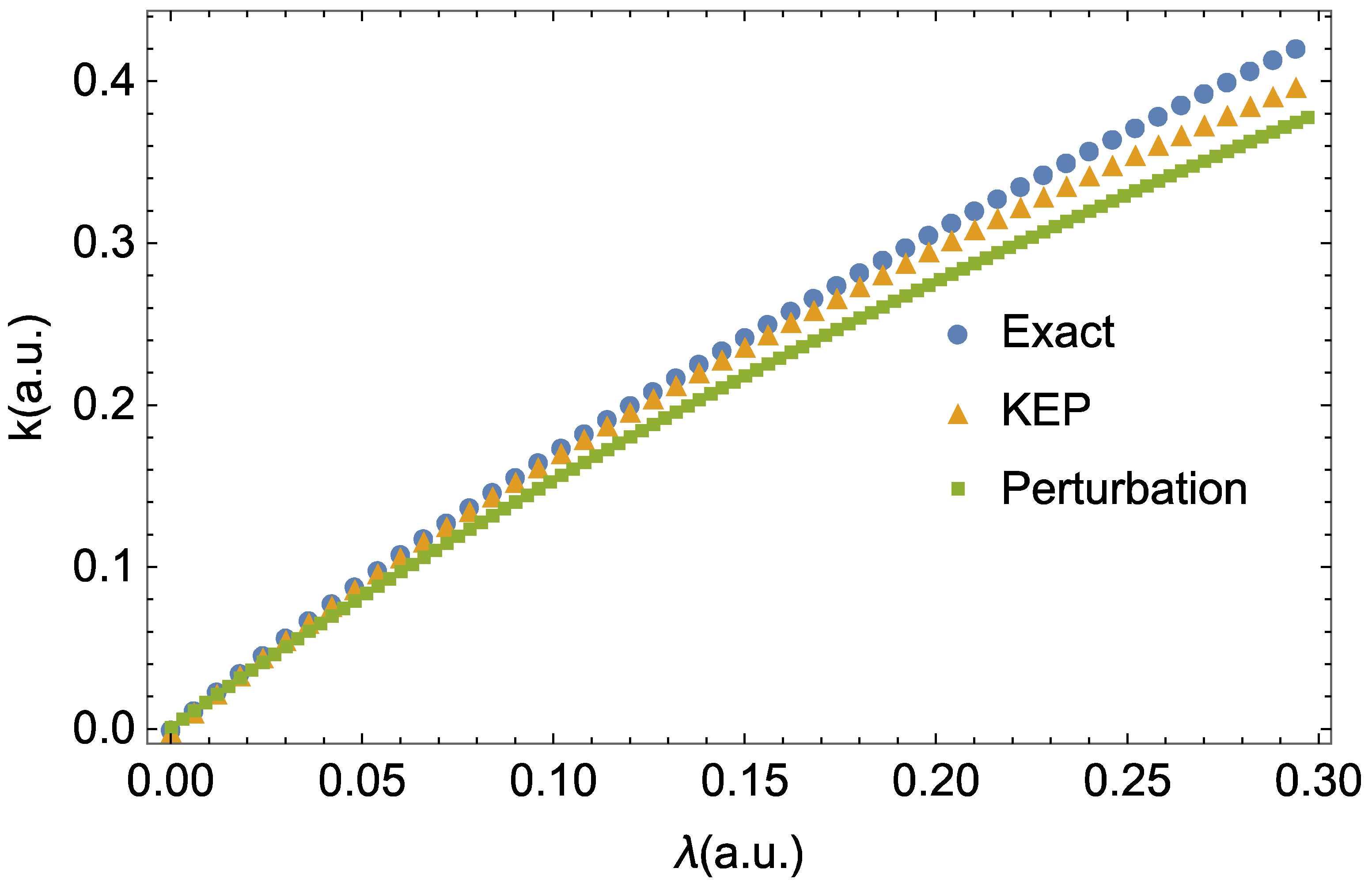
4.1. Double Zero-Range Potentials in One-Dimensional System

The Hamiltonian for the double zero-range potentials could be written as

$$\widehat{H}=-\frac{{\hslash }^2}{2m}\frac{{\partial }^2}{\partial x^2}-{\lambda }_1\delta \left(x+a\right)-{\lambda }_2\delta \left(x-a\right).$$

(45)

If ${\lambda }_1={\lambda }_2=\lambda >0$, this system is symmetric with respect to the origin. By using the KEP method, Equation (45) can be rewritten as

$$\widehat{H}={\widehat{H}}_1+{\widehat{H}}_2=\left[-\frac{{\hslash }^2}{2m_1}\frac{{\partial }^2}{\partial x^2}-{\lambda }_1\delta \left(x_1+a\right)\right]+\left[-\frac{{\hslash }^2}{2m_2}\frac{{\partial }^2}{\partial x^2}-{\lambda }_2\delta \left(x_2-a\right)\right],$$

(46)

where the partitioning mass is $m_1=m_2=2m.$ The Schrödinger equation for each subsystem is ${\widehat{H}}_i{\psi }_i\left(x\right)=E_i{\psi }_i\left(x\right)$ and $E_i=-\left(2m\right){\lambda }^2/\left(2{\hslash }^2\right)$. The wave functions of subsystems ${\widehat{H}}_1$ and ${\widehat{H}}_2$ are

$${\psi }_1\left(x\right)=\left\{\begin{array}{c}\sqrt{k}\exp \left[k\left(x-a\right)\right], x<a\\ \sqrt{k}\exp \left[-k\left(x-a\right)\right], x>a \end{array}\right.,$$

$${\psi }_2\left(x\right)=\left\{\begin{array}{c}\sqrt{k}\exp \left[k\left(x+a\right)\right], x<-a\\ \sqrt{k}\exp \left[-k\left(x+a\right)\right], x>-a \end{array}\right.,$$

(47)

where the wave number $k$ is

$$k=\frac{\left(2m\right)\lambda }{{\hslash }^2}=\sqrt{-\frac{2\left(2m\right)E_1}{{\hslash }^2}}$$

(48)

According to Equation (16), the KEP energy $E_{\mathrm{K}\mathrm{E}\mathrm{P}}$ and KEP wave number $k_{\mathrm{K}\mathrm{E}\mathrm{P}}$ could be written as

$$E_{\mathrm{K}\mathrm{E}\mathrm{P}}=2E_1+\frac{\xi }{1+\eta }=-\frac{{\hslash }^2{k}_{\mathrm{K}\mathrm{E}\mathrm{P}}^2}{2m}$$

(49)

where the overlap coupling matrices $\xi$ and $\eta$ are

$$\xi =\lambda k \left[1-\exp \left(-4ka\right)\right]$$

$$\eta =\exp \left(-2ka\right)\left(2ka+1\right)$$

(50)

Figure 1 presents a comparative analysis of the exact wave numbers and those obtained via the kinetic energy partition (KEP) method against the strength of a zero-range potential, denoted by λ. This comparison elucidates the correlation between precise quantum mechanical calculations and the KEP approach on the one hand and the perturbation method on the other as λ varies. Based on the description and the visual representation provided in Figure 1, it can be observed that when the strength of the zero-range potential, λ, is small, the wave numbers calculated using the kinetic energy partitioning (KEP) method align closely with those derived from exact quantum mechanical solutions. This indicates a high degree of accuracy of the KEP method in the regime of weak potentials. The data points, represented by blue dots, are nearly indistinguishable from the exact solution, signifying strong agreement. The results of using the first-order perturbation method, by treating one delta potential as perturbation, are represented by green squares. The first-order perturbation method shows reasonable agreement with the exact solutions at lower values of λ; yet, as λ increases, the perturbation approximations begin to diverge, suggesting its limitations in the context of stronger potentials. However, as λ increases, the potential becomes stronger, and while the general trend of the KEP method continues to follow the exact solutions, there is a slight divergence noted, which might be indicative of the limits of KEP approximation under the conditions of strong interactions. The KEP method significantly deviates from the exact solution, emphasizing the need for careful application of the KEP method at certain ranges of λ. The overall linear trend suggests a proportional relationship between the wave numbers and the strength of the potential across a wide range of λ values. Figure 2 shows the wave function profiles obtained with the kinetic energy partitioning (KEP) method and exact calculations within the domain $x\in \left[-3, 3\right] (a.u.)$. The graph features a dual-peak structure (that is, the discontinuity in the first derivatives of the wave function), which reflects the divergent behavior of the zero-range potential. The KEP method demonstrates high accuracy in the wave function form, as evidenced by its close approximation to the exact wave function.

4.2. Triple Zero-Range Potentials in One-Dimensional System

In this subsection, the KEP method is tested by extending the double zero-range potential to the triple zero-range potential. The Hamiltonian with the triple zero-range interaction can be represented as

$$\widehat{H}=-\frac{{\hslash }^2}{2m}\frac{{\partial }^2}{\partial x^2}-{\lambda }_1\delta \left(x+a\right)-{\lambda }_2\delta \left(x\right)-{\lambda }_3\delta (x-a).$$

(51)

Here, we consider a case where the interactions are of equal strengths and are all attractive, namely ${\lambda }_1={\lambda }_2={\lambda }_3=\lambda >0$. Based on the KEP method, the sub-Hamiltonian can be separated with the equal mass partition, $m_i=3m$ $\left(i=1, 2, 3\right)$,

$$\widehat{H}={\widehat{H}}_1+{\widehat{H}}_2+{\widehat{H}}_3$$

(52)

where the respective subsystem’s Hamiltonian is

$$\begin{gathered} {\widehat{H}}_1=-\frac{{\hslash }^2}{2m_1}\frac{{\partial }^2}{\partial x^2}-{\lambda }_1\delta \left(x+a\right) \\ {\widehat{H}}_2=-\frac{{\hslash }^2}{2m_2}\frac{{\partial }^2}{\partial x^2}-{\lambda }_2\delta \left(x\right) \\ {\widehat{H}}_3=-\frac{{\hslash }^2}{2m_3}\frac{{\partial }^2}{\partial x^2}-{\lambda }_3\delta \left(x-a\right) \end{gathered}$$

(53)

The KEP energies can be obtained by solving the determinant of Equation (9) involving the overlap coupling matrix $\xi$ and $\eta$.

Figure 3 and Figure 4 collectively offer a comprehensive insight into the behavior of wave numbers and wave function amplitudes in a system characterized by a triple zero-range potential. In Figure 3, a meticulous comparison between the exact wave numbers and those obtained through the kinetic energy partition (KEP) method is depicted, with varying λ values symbolizing the strength of interaction. The exact wave numbers are indicated by blue circles, while the KEP-derived wave numbers are represented by orange triangles. As the λ value, measured in the atomic unit, escalates, both the exact and KEP wave numbers maintain a linear correlation, suggesting a proportional relationship between the wave number $k$, also in the atomic unit, and the interaction strength. The close proximity of the KEP points to the exact values at lower λ indicates a high precision of the KEP method in this regime. With increasing λ, slight deviations become apparent, signaling the nuanced complexity captured by the KEP method under stronger interactions.

Figure 4 shows the probability amplitude ${\left|\psi \right|}^2$ within the spatial domain of $x\in \left[-3, 3\right]$ in the atomic units, showcasing the wave function profiles generated by both the KEP method and exact calculations. The solid blue line traces the KEP probability amplitude, while the dashed orange line delineates the exact solution. The triple peaks observed in the graph correspond to the divergent nature of the triple zero-range potential. The remarkable agreement between the two methods demonstrates KEP’s adeptness at accurately capturing the wave function’s intricate structure.

4.3. N Harmonic Oscillator Interactions in One-Dimensional Schrödinger Equation

The system of a particle interacting with many harmonic oscillator interactions [13,16,17,18,19] in a one-dimensional space serves as a good example for modeling the local dynamics of a defect in solid-state materials [20,21]. Here, the KEP method is used to study this model system. The Hamiltonian for a quantum system with many harmonic interactions can be represented as

$$\widehat{H}=\frac{{\widehat{p}}^2}{2m}+\frac{1}{2}\sum _{i=1}^N{k}_i{\left(x-d_i\right)}^2,$$

(54)

where $k_i$ and $d_i$ are the spring constants and equilibrium distances for the subsystem. According to the KEP scheme, kinetic energy can be equally separated into N terms, and the Hamiltonian can be rewritten as

$$\widehat{H}=\sum _{i=1}^N{\widehat{H}}_i=\sum _{i=1}^N\left[\frac{{\widehat{p}}^2}{2m_i}+\frac{1}{2}{k}_i{\left(x-d_i\right)}^2\right],$$

(55)

where the mass is

$${\sum }_{i=1}^N\frac{1}{m_i}=\frac{1}{m}.$$

(56)

The Schrödinger equation corresponding to Equation (54) is $\widehat{H}\psi =E\psi$. The eigenvalue of Equation (55) could be calculated by using Equation (9) for $N$ harmonic interaction in a one-dimensional particle. Plugging the desired eigenvalue into Equation (9), the coefficient set of $\{C_1, C_2,\dots ,C_N\}$ can be found. Finally, the KEP eigenfunction can be written as

$${\psi }^{\mathrm{K}\mathrm{E}\mathrm{P}}=C_1{\psi }_1+C_2{\psi }_2+\dots +C_N{\psi }_N.$$

(57)

The exact solutions for the eigenvalue and eigenfunction of Equation (54) are known

$$\begin{gathered} E_n=\left(n+\frac{1}{2}\right)\hslash \sqrt{\frac{k}{m}}+\frac{k}{2}{\left(\Delta d\right)}^2, n=0, 1, 2, \dots \\ {\psi }_n\left(x\right)={\phi }_n\left(x-\overline{d}\right), \end{gathered}$$

(58)

where ${\phi }_n\left(x\right)$ is the wave function of a simple harmonic oscillator $\left({\widehat{p}}^2/2m+k{x}^2/2\right){\phi }_n\left(x\right)=e_n{\phi }_n\left(x\right)$. $\overline{d}$ and $\Delta d$ can be represented as

$$\begin{gathered} \overline{d}=\frac{1}{k}\sum _{i=1}^N{k}_i{d}_i \\ {\left(\Delta d\right)}^2=\frac{1}{k}\sum _{i=1}^N{k}_i{d}_i^2-{\left(\frac{1}{k}\sum _{i=1}^N{k}_i{d}_i\right)}^2 \end{gathered}$$

(59)

$d_{2i+1}=-\left(i+1\right)d$ and $d_{2i}=i\times d$ are represented as $N\in odd$ and $N\in even$, respectively. We appreciate Dr. Francisco M. Fernaández [14] for pointing out several simplifications in our previous studies [4], giving many useful suggestions and indicating the exact solutions of Equation (58).

Table 1. Comparison of the KEP and exact eigenvalues (in the atomic units) from $N=1$ to $N=10$. The parameters are set as $d_i=0.1\ast \left(N-1\right)$, $k=0.1$ and $m=\hslash =e=1$.

N	KEP (a.u.)	Exact (a.u.)	Error (%)
1	0.15811	0.15811	0
2	0.22386	0.22386	0
3	0.27486	0.27486	0
4	0.31873	0.31873	0
5	0.35848	0.35855	0.0195
6	0.39419	0.39605	0.4696
7	0.43236	0.43233	0.0069
8	0.46822	0.46821	0.0021
9	0.50433	0.50434	0
10	0.54154	0.54125	0.0535

shows the high accuracy of using the KEP method in a system with many quantum harmonic oscillator interactions. The numerical results with five-digit decimals are compared with the exact eigenvalues. The KEP method yields an excellent agreement with the exact energies in Equation (58). Figure 5 plots the KEP wave function square with different $N$ values in Equation (57) as compared to the exact probability density. This illustrates that the KEP eigenfunctions are close to the exact eigenfunction in the case of many quantum harmonic interactions.

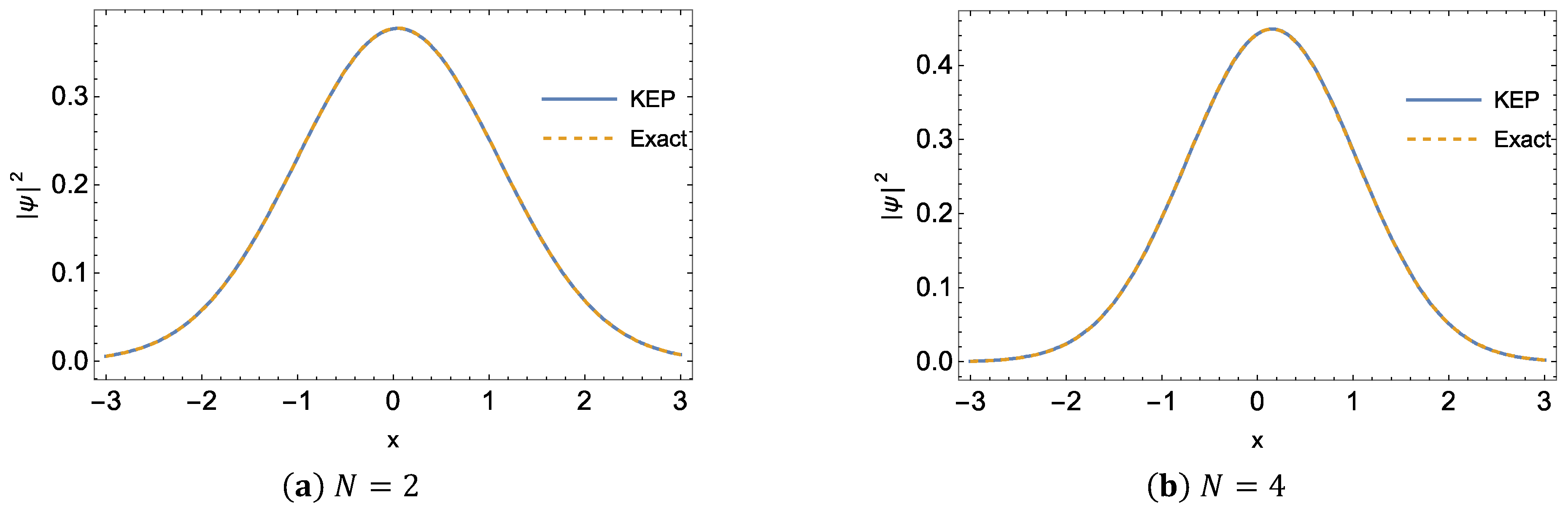
4.4. Three-Body Problem and Many Interactions of One-Dimensional Moshinsky Atoms

In this subsection, we apply the KEP method to a popular atom model—the Moshinsky atom—where harmonic interactions serve as a substitute for the Coulomb interactions among electrons and nuclei. This ideal could help reduce the difficult integrals for the system energy. Recently, the theoretical and experimental progress in our understanding of quasi-one-dimensional cold-atom systems has served as a motivation to study these models [22,23,24,25,26]. The total Hamiltonian of the Moshinsky atom with two electrons is

$$\widehat{H}=\frac{{\widehat{p}}_1^2}{2m}+\frac{1}{2}k{x}_1^2+\frac{{\widehat{p}}_2^2}{2m}+\frac{1}{2}k{x}_2^2-\frac{1}{2}K{\left(x_1-x_2\right)}^2$$

(60)

where $K$ and $k$ are the spring constants for the electron–electron and electron–nucleus interactions, respectively. According to the KEP method [9], we can separate the mass of the kinetic energy terms in Equation (60), and the electron–electron interaction term is divided into two equal parts. The total Hamiltonian can be written as

$$\widehat{H}=-\frac{{\hslash }^2}{2\left(\frac{m}{s_1}\right)}\frac{{\partial }^2}{\partial x_1^2}-\frac{1}{2}\left(\frac{K}{2}\right){\left(x_1-x_2\right)}^2-\frac{{\hslash }^2}{2\left(\frac{m}{1-s_1}\right)}\frac{{\partial }^2}{\partial x_1^2}+\frac{1}{2}k{x}_1^2$$

$$-\frac{{\hslash }^2}{2\left(\frac{m}{s_2}\right)}\frac{{\partial }^2}{\partial x_2^2}-\frac{1}{2}\left(\frac{K}{2}\right){\left(x_1-x_2\right)}^2-\frac{{\hslash }^2}{2\left(\frac{m}{1-s_1}\right)}\frac{{\partial }^2}{\partial x_1^2}+\frac{1}{2}k{x}_1^2$$

$$=\left({\widehat{H}}_{\mathrm{1,2}}+{\widehat{H}}_1\right)+\left({\widehat{H}}_{\mathrm{2,1}}+{\widehat{H}}_2\right)$$

(61)

Notice that Equation (61) contains repulsion interactions; therefore, the adjustable parameters $s_1 \mathrm{a}\mathrm{n}\mathrm{d} s_2$ are set to negative one, which uses the concept of negative mass. The parameters $s_1 \mathrm{a}\mathrm{n}\mathrm{d} s_2$ provide a generalized approach to modulating the mass parameter, thereby introducing additional degrees of freedom to address the complexity inherent in many-body systems. The Schrödinger equations for the four Hamiltonian systems are

$$\left\{\begin{array}{c}{\widehat{H}}_1{\psi }_1=E_1{\psi }_1\\ {\widehat{H}}_{\mathrm{1,2}}{\psi }_{\mathrm{1,2}}=E_{\mathrm{1,2}}{\psi }_{\mathrm{1,2}}\\ {\widehat{H}}_2{\psi }_2=E_2{\psi }_2\\ {\widehat{H}}_{\mathrm{2,1}}{\psi }_{\mathrm{2,1}}=E_{\mathrm{2,1}}{\psi }_{\mathrm{2,1}}\end{array}\right.$$

(62)

The ${\widehat{H}}_1$ and ${\widehat{H}}_2$ partial systems are simply mass-modified ($m\to m_1=m/(1-s_1)$ and $m\to m_2=m/(1-s_2)$) harmonic oscillator potential problems; therefore, the ground state energies and wave functions are both known as

$$\begin{gathered} E_1=\frac{1}{2}\left(2n_1+1\right)\hslash {\omega }_1, n_1=\mathrm{0,1},2,\dots \\ {\psi }_1\left(x_1\right)=\frac{1}{\sqrt{2^{n_1}{n}_1!}}{\left(\frac{2b_1}{\pi }\right)}^{1/4}\exp \left(-b_1{x}_1^2\right)H_{n_1}\left(\sqrt{2b_1}{x}_1\right) \end{gathered}$$

(63)

$$\begin{gathered} E_2=\frac{1}{2}\left(2n_2+1\right)\hslash {\omega }_2, n_1=\mathrm{0,1},2,\dots \\ {\psi }_2\left(x_2\right)=\frac{1}{\sqrt{2^{n_2}{n}_2!}}{\left(\frac{2b_2}{\pi }\right)}^{1/4}\exp \left(-b_2{x}_2^2\right)H_{n_2}\left(\sqrt{2b_2}{x}_2\right) \end{gathered}$$

(64)

where ${\omega }_1=\sqrt{k/m_1}$, $\omega =\sqrt{k/m_2}$, $H_n\left(x\right)$ are the n-th order Hermite polynomials, and $b_1$, $b_2$ is defined as

$$b_1=\frac{m_1{\omega }_1}{2\hslash };b_2=\frac{m_2{\omega }_2}{2\hslash }$$

(65)

Then, we solve the ${\widehat{H}}_{\mathrm{1,2}}$ partial system, for which the Schrödinger equation is

$$\left[-\frac{{\hslash }^2}{2\left(\frac{m}{s_1}\right)}\frac{{\partial }^2}{\partial x_1^2}-\frac{1}{2}\left(\frac{K}{2}\right){\left(x_1-x_2\right)}^2\right]{\psi }_{\mathrm{1,2}}=E_{\mathrm{1,2}}{\psi }_{\mathrm{1,2}}$$

(66)

Through the momentum translation invariance, let $\rho \equiv \left|x_1-x_2\right|$ to perform the variable transformation. Notice that because the interaction potential is an inverse (repulsive) harmonic oscillator, the system is unstable. However, if we choose to use a negative mass, namely s₁ < 0, it also becomes an effective (attractive) harmonic oscillator problem due to the negative mass.

$$\left[-\frac{{\hslash }^2}{2\left(\frac{m}{\left|s_1\right|}\right)}\frac{{\partial }^2}{\partial {\rho }_1^2}+\frac{1}{2}\left(\frac{K}{2}\right){\rho }_1^2\right]{\psi }_{\mathrm{1,2}}\left({\rho }_1\right)=-E_{\mathrm{1,2}}{\psi }_{\mathrm{1,2}}\left({\rho }_1\right)$$

(67)

This is the reason why we can avoid using the continuous-energy basis sets associated with the original repulsion interaction. We obtain the ground state energy and wave function by shifting the origin to $x_2$:

$$E_{\mathrm{1,2}}=-\frac{1}{2}\left(2n_{\mathrm{1,2}}+1\right)\hslash {\omega }_{\mathrm{1,2}} n_{\mathrm{1,2}}=\mathrm{0,1},2,\dots$$

(68)

$${\psi }_{\mathrm{1,2}}\left({\rho }_1\right)=\frac{1}{\sqrt{2^{n_{\mathrm{1,2}}}{n}_{\mathrm{1,2}}!}}{\left(\frac{2b_{\mathrm{1,2}}}{\pi }\right)}^{\frac{1}{4}}\exp \left(-b_{\mathrm{1,2}}{\rho }_1^2\right)H_{n_{\mathrm{1,2}}}\left(\sqrt{2b_{\mathrm{1,2}}}{\rho }_1\right)$$

(69)

Notice that $m_{\mathrm{1,2}}=m/\left|s_1\right|$, and $H_n\left(x\right)$ is the n-th order Hermite polynomial. Additionally, $b_{\mathrm{1,2}}$ and ${\omega }_{\mathrm{1,2}}$ are defined as

$$b_{\mathrm{1,2}}=\frac{m_{\mathrm{1,2}}{\omega }_{\mathrm{1,2}}}{2\hslash }, {\omega }_{\mathrm{1,2}}=\sqrt{K/2m_{\mathrm{1,2}}}$$

(70)

The energy and wave function of the partial system ${\widehat{H}}_{\mathrm{2,1}}$ can be obtained with the same method described above by simply exchanging the indices. Next, we solve the Schrödinger equation with the subsystem Hamiltonian ${\widehat{K}}_1$:

$${\widehat{K}}_1{\varphi }_1={\epsilon }_1{\varphi }_1$$

(71)

where

$${\widehat{K}}_1={\widehat{H}}_{\mathrm{1,2}}+{\widehat{H}}_1$$

(72)

Now, we assume that the wave function of the subsystem for electron one is a linear combination of ${\psi }_{\mathrm{1,2}}\left({\rho }_1\right)$ and ${\psi }_1\left(x_1\right)$:

$${\varphi }_1\left(x_1;x_2\right)=C_{\mathrm{1,2}}{\psi }_{\mathrm{1,2}}\left({\rho }_1\right)+C_1{\psi }_1\left(x_1\right)$$

(73)

Substituting Equation (73) into Equation (72), we acquire

$$\left\{\begin{array}{c}{C}_1\left(E_1+{\xi }_{\mathrm{1,2}}-{\epsilon }_1\right)+C_{\mathrm{1,2}}\left(E_1+E_{\mathrm{1,2}}-{\epsilon }_1\right){\eta }_1=0\\ C_1\left(E_1+E_{\mathrm{1,2}}-{\epsilon }_1\right){\eta }_1+C_{\mathrm{1,2}}\left(E_1+{\xi }_{\mathrm{1,2}}-{\epsilon }_1\right)=0\end{array}\right.$$

(74)

The energy of the subsystem ${\widehat{K}}_1$ is obtained by the vanishing determinant of the coefficient matrix:

$${\epsilon }_1^{\pm }\left(x_2\right)=\frac{\left[\left(1-2{\eta }_1^2\right)E_1+\left(1-{\eta }_1^2\right)E_{\mathrm{1,2}}+{\xi }_1+{\xi }_{\mathrm{1,2}}\right]\pm \sqrt{D_1}}{2\left(1-{\eta }_1^2\right)}$$

(75)

where

$$D_1={\left[\left(1-2{\eta }_1^2\right)E_1+\left(1-{\eta }_1^2\right)E_{\mathrm{1,2}}+{\xi }_1+{\xi }_{\mathrm{1,2}}\right]}^2-4\left(1-{\eta }_1^2\right)\left[\left(E_1+{\xi }_{\mathrm{1,2}}\right)\left(E_{\mathrm{1,2}}+{\xi }_1\right)-{\eta }_1^2{\left(E_1+E_{\mathrm{1,2}}\right)}^2\right]$$

(76)

The symbols ${\eta }_1$, ${\xi }_1$ and ${\xi }_{\mathrm{1,2}}$ in Equation (75) are defined and calculated as

$${\eta }_1=⟨{\psi }_{\mathrm{1,2}}|{\psi }_1⟩={\left[\frac{4b_1{b}_{\mathrm{1,2}}}{{\left(b_1+b_{\mathrm{1,2}}\right)}^2}\right]}^{1/4}\exp \left(-\frac{b_1{b}_{\mathrm{1,2}}{x}_2^2}{b_1+b_{\mathrm{1,2}}}\right)$$

(77)

$${\xi }_1=⟨{\psi }_{\mathrm{1,2}}|{\widehat{H}}_1|{\psi }_{\mathrm{1,2}}⟩=-2E_{\mathrm{1,2}}-\frac{K-k\left(1+4b_{\mathrm{1,2}}{x}_2^2\right)}{8b_{\mathrm{1,2}}}$$

(78)

$${\xi }_{\mathrm{1,2}}=⟨{\psi }_1|{\widehat{H}}_{\mathrm{1,2}}|{\psi }_1⟩=-\frac{1}{2}{E}_1+\frac{k-K\left(1+4b_1{x}_2^2\right)}{16b_1}$$

(79)

All of the above symbols are functions of $x_2$. Here, ${\epsilon }_1^{-}\left(x_2\right)$ conforms to the ground state energy; therefore, we will ignore its superscript for simplicity. The normalized wave function is

$${\varphi }_1\left(x_1;x_2\right)=\sqrt{\frac{1}{{\Delta }_1^2+2{\eta }_1{\Delta }_1+1}}\left[{\psi }_1\left(x_1\right)+{\Delta }_1{\psi }_{\mathrm{1,2}}\left({\rho }_1\right)\right]$$

(80)

where

$${\Delta }_1=-\frac{\left(E_1+{\xi }_{\mathrm{1,2}}-{\epsilon }_1\right)}{\left(E_1+E_{\mathrm{1,2}}-{\epsilon }_1\right){\eta }_1 }$$

(81)

Note that the coefficients depending on $x_2$ are obtained by Equation (77) and the normalization condition. The same method can be used to calculate the energy and wave function for electron two by simply swapping the indices $1\leftrightarrow 2$. To solve the full Schrödinger equation

$$\widehat{H}\mathsf{\Psi }=E\mathsf{\Psi }$$

(82)

where

$$\widehat{H}={\widehat{K}}_1+{\widehat{K}}_2$$

(83)

we assume that the total wave function is a Hartree-like product function

$$\mathsf{\Psi }={\varphi }_1\left(x_1;x_2\right)\varphi \left(x_2;x_1\right)$$

Substituting the above equation into Equation (82), we obtain the KEP energy

$$\begin{gathered} E^{\mathrm{K}\mathrm{E}\mathrm{P}}=\iint {\varphi }_1^{*}\left(x_1;x_2\right){\varphi }_2^{*}\left(x_2;x_1\right)\left({\widehat{K}}_1+{\widehat{K}}_2\right){\varphi }_1\left(x_1;x_2\right){\varphi }_2\left(x_2;x_1\right)d{x}_{1}d{x}_2 \\ =2\iint {\varphi }_1^{*}\left(x_1;x_2\right){\varphi }_2^{*}\left(x_2;x_1\right){\widehat{K}}_1{\varphi }_1\left(x_1;x_2\right){\varphi }_2\left(x_2;x_1\right)d{x}_{1}d{x}_2 \end{gathered}$$

(84)

Here, we considered the electron exchange symmetry. The last integral can be written explicitly as

$$\begin{gathered} \iint {\varphi }_1^{*}\left(x_1;x_2\right){\varphi }_2^{*}\left(x_2;x_1\right){\widehat{K}}_1{\varphi }_1\left(x_1;x_2\right){\varphi }_2\left(x_2;x_1\right)d{x}_{1}d{x}_2=\iint d{x}_{1}d{x}_2{\varphi }_1^{*}{\varphi }_2^{*}\left(\frac{{\widehat{p}}_1^2}{2m}+V_1+V_{\mathrm{1,2}}\right){\varphi }_1{\varphi }_2 \\ =\iint d{x}_{1}d{x}_2{\varphi }_1^{*}{\varphi }_2^{*}\left(\frac{{\widehat{p}}_1^2}{2m}{\varphi }_1\right){\varphi }_2+\iint d{x}_{1}d{x}_2{\varphi }_1^{*}{\varphi }_2^{*}\left(\frac{{\widehat{p}}_1^2}{2m}{\varphi }_2\right){\varphi }_1+\iint d{x}_{1}d{x}_2{\varphi }_1^{*}{\varphi }_2^{*}\left(\frac{{\widehat{p}}_1{\varphi }_1{\widehat{p}}_1{\varphi }_2}{m}\right) \\ +\iint d{x}_{1}d{x}_2{\varphi }_1^{*}{\varphi }_2^{*}\left(V_1+V_{\mathrm{1,2}}\right){\varphi }_1{\varphi }_2 \\ =\iint d{x}_{1}d{x}_2{\varphi }_1^{*}{\varphi }_2^{*}{\epsilon }_1\left(x_2\right){\varphi }_1\left(x_1;x_2\right){\varphi }_2\left(x_2;x_1\right)+\iint d{x}_{1}d{x}_2{\varphi }_1^{*}{\varphi }_2^{*}\left(\frac{{\widehat{p}}_1^2}{2m}{\varphi }_2\right){\varphi }_1+\iint d{x}_{1}d{x}_2{\varphi }_1^{*}{\varphi }_2^{*}\left(\frac{{\widehat{p}}_1{\varphi }_1{\widehat{p}}_1{\varphi }_2}{m}\right) \end{gathered}$$

(85)

To simplify Equation (84), we adopt the adiabatic approximation

$$\begin{gathered} \iint d{x}_{1}d{x}_2{\varphi }_1^{*}\left(x_1;x_2\right){\varphi }_2^{*}\left(x_2;x_1\right){\widehat{K}}_1{\varphi }_1\left(x_1;x_2\right){\varphi }_2\left(x_2;x_1\right) \\ \approx \iint {\varphi }_1^{*}{\varphi }_2^{*}{\epsilon }_1\left(x_2\right){\varphi }_1{\varphi }_{2}d{x}_{1}d{x}_2 \end{gathered}$$

(86)

These integrals can be calculated by using the known analytic functions. In

Table 2. Comparison of the exact energy solutions, the KEP and AKEP solutions for the ratio of the spring constants. Here, we utilize the atomic units $m=\hslash =e=1$ and $K=0.01$.

k/K	KEP	AKEP	Exact	Error for KEP (%)	Error for AKEP (%)
2.0	0.101	0.098	0.071	42.5	39.13
2.1	0.106	0.103	0.088	19.6	17.1
2.5	0.123	0.121	0.114	7.6	6.1
3.0	0.142	0.141	0.137	4.2	3.2
3.5	0.160	0.158	0.155	3.1	2.3
4.0	0.175	0.174	0.171	2.6	2.0
4.5	0.190	0.189	0.185	2.4	1.9
5.0	0.203	0.202	0.198	2.4	1.9
5.5	0.216	0.215	0.211	2.4	2.0
6.0	0.228	0.227	0.223	2.4	2.1
6.5	0.239	0.239	0.234	2.5	2.2
8.0	0.271	0.270	0.264	2.7	2.4
10.0	0.308	0.308	0.300	2.9	2.8

, we compare the exact energy, the adiabatic KEP (AKEP) energy and the KEP energy for a range of the ratio of $k/K$. The analytic exact energy is taken from Ref [27].

$$E^{\mathrm{e}\mathrm{x}\mathrm{a}\mathrm{c}\mathrm{t}}=\frac{1}{2}\sqrt{\frac{k-2K}{m}}+\frac{1}{2}\sqrt{\frac{k}{m}}=\frac{1}{2}\sqrt{\frac{k}{m}}\left(\sqrt{1-\frac{2K}{k}}+1\right)$$

(87)

In Equation (84), we can see that the ratio of 2 is a critical point of the exact solution, where the repulsive potential is equivalent to the attractive potential, and the system starts to become unstable. We see that both the KEP and the AKEP results exhibit quite large errors near the critical point, with others being less than 3%. In Figure 6, we plot the exact, KEP and AKEP energies with different k/K ratios. Clearly, the KEP method can be used for a very wide range of $k/K$ ratios. The exact wave function is compared with the KEP solution, as shown in Figure 7. We see an overall agreement in the contour plots, thus demonstrating the feasibility of using the KEP method in modeling the wave functions.

5. Conclusions

In this paper, we review the general methodology of using the recently proposed KEP method for solving quantum eigenvalue problems. The KEP scheme is successfully applied in several illustrative quantum mechanical systems with a wide range of interaction patterns. Using the KEP solution scheme, the symmetry or anti-symmetry of interaction within the particles can be considered. The problems of the symmetric double and triple zero-range potentials are solved with the KEP method, and the KEP energies and wave functions are very close to the exact solutions. The system with N harmonic oscillator interactions is well tested from N = 1 to N = 10, where the KEP method renders an excellent agreement with the exact solutions. Finally, the KEP method is applied to the Moshinsky atom, which is a three-body scenario, and achieves high-accuracy results. Therefore, we demonstrate the high potential of using the KEP method to calculate both the eigenvalues and wave functions for general quantum mechanical problems.

References

1. Arteca, G.A.; Fernández, F.M.; Castro, E.A.; Arteca, G.A.; Fernández, F.M.; Castro, E.A. Large Order Perturbation Theory and Summation Methods in Quantum Mechanics; Springer: Berlin/Heidelberg, Germany, 1990. [Google Scholar]
2. Chen, Y.H.; Greene, C.H. P-wave Efimov physics implications at unitarity. Phys. Rev. A 2023, 107, 033329. [Google Scholar] [CrossRef]
3. Esry, B.D.; Greene, C.H. Spontaneous spatial symmetry breaking in two-component Bose-Einstein condensates. Phys. Rev. A 1999, 59, 1457–1460. [Google Scholar] [CrossRef]
4. Higgins, M.D.; Greene, C.H. Three and four identical fermions near the unitary limit. Phys. Rev. A 2022, 106, 023304. [Google Scholar] [CrossRef]
5. Andrews, D.L. Symmetry and quantum features in optical vortices. Symmetry 2021, 13, 1368. [Google Scholar] [CrossRef]
6. Fernandez, F.M. Introduction to Perturbation Theory in Quantum Mechanics; CRC Press: Boca Raton, FL, USA, 2000. [Google Scholar]
7. Higgins, M.D.; Greene, C.H.; Kievsky, A.; Viviani, M. Nonresonant density of states enhancement at low energies for three or four neutrons. Phys. Rev. Lett. 2020, 125, 052501. [Google Scholar] [CrossRef]
8. Znojil, M. Perturbation theory near degenerate exceptional points. Symmetry 2020, 12, 1309. [Google Scholar] [CrossRef]
9. Mineo, H.; Chao, S.D. Split kinetic energy method for quantum systems with competing potentials. Ann. Phys. 2012, 327, 2061–2073. [Google Scholar] [CrossRef]
10. Chen, Y.; Chao, S.D. Negative Mass Can Be Positively Useful in Quantum Mechanics. J. Chin. Chem. Soc. 2018, 65, 654–666. [Google Scholar] [CrossRef]
11. Chen, Y.-H.; Chao, S.D. The kinetic energy partition method applied to a confined quantum harmonic oscillator in a one-dimensional box. Chin. J. Phys. 2018, 56, 584–592. [Google Scholar] [CrossRef]
12. Chen, Y.-H.; Chao, S.D. Kinetic energy partition method applied to ground state helium-like atoms. J. Chem. Phys. 2017, 146, 124120. [Google Scholar] [CrossRef]
13. Benavides-Riveros, C.L.; Toranzo, I.V.; Dehesa, J.S. Entanglement in N-harmonium: Bosons and fermions. J. Phys. B At. Mol. Opt. Phys. 2014, 47, 195503. [Google Scholar] [CrossRef]
14. Fernández, F.M. Comment on: “The kinetic energy partition method applied to quantum eigenvalue problems with many harmonic-oscillator potentials” by Y.-H. Chen and SD Chao. J. Math. Chem. 2018, 56, 1511–1514. [Google Scholar] [CrossRef]
15. Chen, Y.-H.; Chao, S.D. Solving many-body Schrödinger equations with kinetic energy partition method. Ann. Phys. 2018, 388, 54–68. [Google Scholar] [CrossRef]
16. Armstrong, J.R.; Volosniev, A.G.; Fedorov, D.V.; Jensen, A.S.; Zinner, N.T. Analytic solutions of topologically disjoint systems. J. Phys. A Math. Theor. 2015, 48, 085301. [Google Scholar] [CrossRef]
17. Mehta, N.P. Born-Oppenheimer study of two-component few-particle systems under one-dimensional confinement. Phys. Rev. A 2014, 89, 052706. [Google Scholar] [CrossRef]
18. Armstrong, J.R.; Zinner, N.T.; Fedorov, D.V.; Jensen, A.S. Analytic harmonic approach to the N-body problem. J. Phys. B At. Mol. Opt. Phys. 2011, 44, 055303. [Google Scholar] [CrossRef]
19. Alon, O.E. Analysis of a trapped Bose–Einstein condensate in terms of position, momentum, and angular-momentum variance. Symmetry 2019, 11, 1344. [Google Scholar] [CrossRef]
20. Vitória, R.L.L.; Belich, H. Harmonic oscillator in an environment with a pointlike defect. Phys. Scr. 2019, 94, 125301. [Google Scholar] [CrossRef]
21. Pattanayak, A.; Dixit, G. Influence of vacancy defects in solid high-order harmonic generation. Phys. Rev. A 2020, 101, 013404. [Google Scholar] [CrossRef]
22. Kościk, P.; Kuroś, A.; Pieprzycki, A.; Sowiński, T. Pair-correlation ansatz for the ground state of interacting bosons in an arbitrary one-dimensional potential. Sci. Rep. 2021, 11, 13168. [Google Scholar] [CrossRef]
23. Wan, J.-Y.; Wang, X.; Zhang, X.; Meng, Y.-L.; Wang, W.-L.; Sun, Y.; Liu, L. Quasi-one-dimensional diffuse laser cooling of atoms. Phys. Rev. A 2022, 105, 033110. [Google Scholar] [CrossRef]
24. Kościk, P. Quantum entanglement of two harmonically trapped dipolar particles. Few-Body Syst. 2015, 56, 107–114. [Google Scholar] [CrossRef]
25. Mistakidis, S.; Volosniev, A.; Barfknecht, R.; Fogarty, T.; Busch, T.; Foerster, A.; Schmelcher, P.; Zinner, N. Few-body Bose gases in low dimensions—A laboratory for quantum dynamics. Phys. Rep. 2023, 1042, 1–108. [Google Scholar] [CrossRef]
26. Greene, C.H.; Giannakeas, P.; Pérez-Ríos, J. Universal few-body physics and cluster formation. Rev. Mod. Phys. 2017, 89, 035006. [Google Scholar] [CrossRef]
27. Cohen, L.; Lee, C. Exact reduced density matrices for a model problem. J. Math. Phys. 1985, 26, 3105–3108. [Google Scholar] [CrossRef]
Figure 1. Comparison of the exact, KEP and perturbation method of wave numbers versus the λ values for the double zero-range potential, where the strengths of interaction are the same. The (blue) circle, (orange) triangle and (green) square represent the exact and the KEP wave numbers, respectively. The x-axis is the λ value in the atomic unit, and the y-axis is the wave number k in the atomic unit, and here, a = 1 .
Symmetry 16 00290 g001
Figure 2. Illustration of the KEP and exact probability amplitudes ψ 2 within x 3 ,   3   a . u . and λ = 0.15   ( a . u . ) for the double zero-range potential. The solid (blue) line and dashed (orange) line are the KEP and exact solutions, respectively.
Symmetry 16 00290 g002
Figure 3. Comparison of the exact and KEP wave numbers versus the λ values for the triple zero-range potential, where the strengths of interaction are the same. The (blue) circle and (orange) triangle represent the exact and KEP wave numbers, respectively. The horizontal axis is the λ value in the atomic unit, and the vertical axis is the wave number k in the atomic unit, and here, a = 1 .
Symmetry 16 00290 g003
Figure 4. Illustration of the KEP and exact probability amplitudes ψ 2 within x 3 ,   3   a . u . and λ = 0.1 for the triple zero-range potential. The solid (blue) line and dashed (orange) line are the KEP and exact solutions, respectively.
Symmetry 16 00290 g004
Figure 5. Illustration of the KEP and exact wave functions with the double and quadruple harmonic interactions, respectively. The parameters are set as d i = 0.1 N 1 , k = 0.1 and m = = e = 1 .
Symmetry 16 00290 g005
Figure 6. Comparison of the exact, KEP and AKEP energies with the k/K ratio from 2 to 10 for the two-electron Moshinsky atom in the atomic units.
Symmetry 16 00290 g006
Figure 7. Illustration of the contour plots of the exact wave function and the KEP solution for the Moshinsky atom with the interaction ratio k/K = 4 in the atomic units.
Symmetry 16 00290 g007