Approximate N⁵LO Higgs Boson Decay Width Γ(H→γγ)

Abstract

The precision and predictive power of perturbative QCD (pQCD) prediction depends on both a precise, convergent, fixed-order series and a reliable way of estimating the contributions of unknown higher-order (UHO) terms. It has been shown that by applying the principle of maximum conformality (PMC), which applies the renormalization group equation recursively to set the effective magnitude of ${\alpha }_s$ of the process, the remaining conformal coefficients will be well matched with the corresponding ${\alpha }_s$ at each order, leading to a scheme-and-scale invariant and more convergent perturbative series. The PMC series, being satisfied with the standard renormalization group invariance, has a rigorous foundation. Thus it not only can be widely applied to virtually all high-energy hadronic processes, but also can be a reliable platform for estimating UHO contributions. In this paper, by using the total decay width $\Gamma (H\to \gamma \gamma )$ which has been calculated up to N⁴LO QCD corrections, we first derive its PMC series by using the PMC single-scale setting approach and then estimate its unknown N⁵LO contributions by using a Bayesian analysis. The newly suggested Bayesian-based approach estimates the magnitude of the UHO contributions based on an optimized analysis of the probability density distribution, and the predicted UHO contribution becomes more accurate when more loop terms have been known to tame the probability density function. Using the top-quark pole mass $M_t$ = 172.69 GeV and the Higgs mass $M_H$ = 125.25 GeV as inputs, we obtain $\Gamma (H\to \gamma \gamma )=9.56504\mathrm{keV}$, and the estimated N⁵LO contribution to the total decay width is $\Delta {\Gamma }_H=\pm 1.65\times {10}^{-4}\mathrm{keV}$ for the smallest credible interval of $95.5\%$ degree of belief.

1. Introduction

The ATLAS and CMS collaborations have discovered the Higgs boson in 2012 [1,2], consistent with the elementary particle suggested by the Standard Model (SM). The Higgs boson answers some of the most profound questions in physics, such as where the masses of the elementary particles and the $W^{\pm }/Z^0$ gauge bosons come from, how the electroweak phase transition governs the evolution of the early universe, etc. It is then crucial to verify and study the Higgs properties, either experimentally or theoretically.

Precise measurements of the Higgs boson production and decay channels provide critical tests of the SM and are vital in the exploration of new physics beyond the SM. Over the past decade, many new measurements on the Higgs boson properties have been performed by the collaborations at the LHC. Some new Higgs factories such as the International Linear Collider (ILC) [3], the Circular Electron Positron Collider (CEPC) [4] and the Future Circular Collider [5] have been designed to further improve the experimental precision on the Higgs properties. Thus, the Higgs boson is being moved from the object of a search to an exploration tool. Till now, almost all of the related measurements have been in agreement with the SM predictions within errors. As one of the most important decay channels of the Higgs boson, it has been shown that the process $H\to \gamma \gamma$ has an observable fraction $(2.50\pm 0.20)\times {10}^{-3}$ [6], which plays an important role in Higgs phenomenology.

Because the photon is massless, the process $H\to \gamma \gamma$ is a loop-induced process even at the leading-order level, whose amplitude can be decomposed into a bosonic contribution, stemming from the W boson, and the fermionic contributions, respectively. More explicitly, its decay width can be written as

$$\begin{array}{c}\hfill \Gamma (H\to \gamma \gamma )=\frac{M_H^3}{64\pi }{\left|A_W+\sum _f{A}_f\right|}^2,\end{array}$$

(1)

where $M_H$ is the Higgs mass, $A_W$ is the contribution from the purely bosonic diagrams, and $A_f$ is the contribution from the amplitudes with $f=(t,b,c,\tau )$, which corresponds to the top quark, the bottom quark, the charm quark, and the $\tau$ lepton, accordingly. The above equation can be further rewritten as [7]

$$\begin{array}{c}\hfill \Gamma (H\to \gamma \gamma )=\frac{M_H^3}{64\pi }\left(A_{\mathrm{LO}}^2+A_{\mathrm{EW}}\frac{\alpha }{\pi }\right)+R_n,\end{array}$$

(2)

where $\alpha$ is the fine-structure constant, $A_{\mathrm{EW}}$ is the electroweak (EW) correction [8,9], $A_{\mathrm{LO}}$ is the leading-order (LO) contribution, and $R_n$ represents the QCD corrections, in which n represents the QCD correction calculated up to the $n_{\mathrm{th}}$-loop level. At present, the LO, the next-to-leading order (NLO), the N²LO, the N³LO, and the N⁴LO perturbative QCD (pQCD) corrections for $\Gamma (H\to \gamma \gamma )$ have been calculated in Refs. [8,9,10,11,12,13,14,15,16,17,18,19,20,21,22,23,24] under various approaches. In particular, the fermionic contribution which forms a gauge-invariant subset has been calculated up to the N⁴LO level in the large top-quark limit with $M_H<<2m_t$ [21]. Those improvements give us a good basis for achieving a precise pQCD prediction on $\Gamma (H\to \gamma \gamma )$. On the other hand, future precise measurements on the Higgs boson decay may determine the branching fraction of its decay into two photons up to a high precision of one percent [25]. Thus, to fully exploit future precise measurements, it is important to achieve a high-precision theoretical prediction as much as possible, as is the purpose of the present paper.

2. The N⁴LO-Level Prediction ${\mathit{R}}_{\mathbf{4}}$ under the PMC and the Higher-Order Contribution Using a Bayesian Analysis

A valid prediction for a physical observable from quantum field theory should be independent of the choice of renormalization scheme and scale—this is the primary requirement of renormalization group invariance (RGI). Satisfying the RGI is a challenging problem for pQCD, since a truncated perturbation series does not automatically satisfy the requirements of the renormalization group. In the following we will take the higher-order QCD corrections to the process $H\to \gamma \gamma$ as an explicit example.

The perturbative series of the QCD correction $R_4$ up to the $\mathcal{O}\left({\alpha }_s^5\right)$ level can be read from Refs. [20,21], which is given in $n_f$ series with $n_f$ being the active number of quark flavors. For the later convenience of applying the renormalization group equation (RGE) to set the effective magnitude of ${\alpha }_s$, we express it as a $\left\{{\beta }_i\right\}$ series by using the general degeneracy relations of the QCD theory among different orders, e.g.,

$$\begin{array}{cc}\hfill R_4=& \sum _{i=1}^4{r}_i({\mu }_r^2/Q^2)a^i\left({\mu }_r\right)\hfill \\ \hfill =& r_{1,0}a\left({\mu }_r\right)+[r_{2,0}+{\beta }_0{r}_{2,1}]a^2\left({\mu }_r\right)\hfill \\ \hfill & +[r_{3,0}+{\beta }_1{r}_{2,1}+2{\beta }_0{r}_{3,1}+{\beta }_0^2{r}_{3,2}]a^3\left({\mu }_r\right)\hfill \\ \hfill & +[r_{4,0}+{\beta }_2{r}_{2,1}+2{\beta }_1{r}_{3,1}+\frac{5}{2}{\beta }_1{\beta }_0{r}_{3,2}+3{\beta }_0{r}_{4,1}\hfill \end{array}$$

(3)

$$\begin{array}{cc}\hfill & +3{\beta }_0^2{r}_{4,2}+{\beta }_0^3{r}_{4,3}]a^4\left({\mu }_r\right)+\mathcal{O}\left(a^5\right),\hfill \end{array}$$

(4)

where $a={\alpha }_s/\pi$ and $Q=M_t$ ($M_t$ being the top-quark pole mass), which represents the typical momentum flow of the process. The $\left\{{\beta }_i\right\}$-functions have been calculated up to the five-loop level in the $\overline{\mathrm{MS}}$ scheme [26,27,28,29,30,31,32,33,34,35,36,37]. The expansion coefficients $r_{i,j}$ in Equation (3) can be derived from the ones of Refs. [20,21] via proper transformations. In Refs. [20,21], the perturbative expressions are given in the form of the $\overline{\mathrm{MS}}$-scheme top-quark running mass $\left(m_t\right)$. Following the arguments of Ref. [38], we transform it into the perturbative series over the top-quark pole mass ($M_t$) with the help of the $O\left({\alpha }_s^5\right)$-level relation between $m_t$ and $M_t$ [22] in order to avoid the confusion of applying the PMC-scale-setting procedures, e.g., only the RGE-involved ${\beta }_i$ terms remain and are adopted for fixing the correct magnitude of the strong coupling and its argument, e.g., the PMC scale $Q^{\ast }$. The coefficients $r_{i,0}$ are conformal ones which are free of the renormalization scale ${\mu }_r$, and the nonconformal coefficients $r_{i,j(\ne 0)}$ are functions of ${\mu }_r$ which can be expressed as

$$\begin{array}{c}\hfill r_{i,j}=\sum _{k=0}^j{C}_j^k{\widehat{r}}_{i-k,j-k}{ln}^k({\mu }_r^2/Q^2),\end{array}$$

(5)

where ${\widehat{r}}_{i,j}=r_{i,j}{|}_{{\mu }_r=Q}$. The RGE determines the running behavior of ${\alpha }_s$ and is scheme-dependent. By applying the principle of maximum conformality (PMC) [39,40,41,42,43], which applies the RGE recursively to set the effective magnitude of ${\alpha }_s$ of the process, the remaining conformal coefficients are well matched with the corresponding ${\alpha }_s$ at each order, leading to a scheme-and-scale invariant and convergent perturbative series free of divergent renormalization terms, cf. the reviews [44,45,46]. These reviews show that the PMC predictions respect all features of the renormalization group, and its prediction satisfies all the requirements of RGI; The commensurate scale relations, which relate physical observables to each other, ensure that PMC predictions are independent of the choice of renormalization scheme for any observable; And the transitivity and symmetry properties of the commensurate scales are the scale transformations of the renormalization “group”. Moreover, the PMC reduces in the Abelian limit to the Gell–Mann–Low method [47], and it provides a solid way to extend the well-known Brodsky–Lepage–Mackenzie (BLM) method [48] to all orders.

The PMC single-scale approach (PMCs) [49] determines an overall effective ${\alpha }_s$ (its argument is called the PMC scale) for the fixed-order predictions, and the resultant perturbative series provide a good basis for demonstrating that the PMC series is free of renormalization scale-and-scheme ambiguities up to any fixed order, being consistent with the fundamental renormalization group approaches [50,51]. It is noted that the single-scale approaches suggested in Ref. [49] are different from each other, but it has been demonstrated that the resultant pQCD series for both approaches are exactly the same. This equivalence indicates that by using the RGE to fix the value of the effective coupling is equivalent to requiring each loop’s terms to be scale-invariant simultaneously. Following the PMCs procedures [49], all the RGE-involved nonconformal terms of the above conventional series (4) of $R_4\left({\mu }_r\right)$ should be removed from the series and adopted for fixing the correct magnitude of ${\alpha }_s$ of the process; one then obtains a scale-invariant conformal series. Up to the N⁴LO level, we have

$$\begin{array}{c}\hfill R_4{|}_{\mathrm{PMCs}}=\sum _{i=1}^4{\widehat{r}}_{i,0}{a}^i\left(Q_{\ast }\right)+\mathcal{O}\left(a^5\right),\end{array}$$

(6)

where $Q_{\ast }$ is the PMC scale, which can be determined by the following equation

$$\begin{array}{ccc}\hfill ln\frac{Q_{\ast ,{\mathrm{N}}^{\mathit{l}}\mathrm{LL}}^2}{Q^2}& =& -\frac{{\sum }_{k=1}^{l+2}{\sum }_{i=1}^{l-k+2}\left[{(-1)}^i{\Delta }_{n,k}^{(i-1)}{\widehat{r}}_{k+i,i}(n+k-1)a^k\left(Q_{\ast ,{\mathrm{N}}^{\mathit{l}}\mathrm{LL}}\right)\right]}{{\sum }_{\eta =1}^{l+1}{\sum }_{k=1}^{l+2}{\sum }_{i=\eta }^{l-k+2}\left[{(-1)}^i(n+k-1)C_i^{\eta }{\Delta }_{n,k}^{(i-1)}{\widehat{r}}_{k+i-\eta ,i-\eta }{L}_{Q_{\ast ,{\mathrm{N}}^{\mathit{l}-\mathit{1}}\mathrm{LL}}}^{\eta -1}{a}^k\left(Q_{\ast ,{\mathrm{N}}^{\mathit{l}}\mathrm{LL}}\right)\right]}\hfill \end{array}$$

(7)

$$\begin{array}{ccc}& =& \sum _{i=0}^2{S}_i{a}^i\left(Q_{\ast ,{\mathrm{N}}^{\mathit{l}}\mathrm{LL}}\right),\hfill \end{array}$$

(8)

where $L_{Q_{\ast ,{\mathrm{N}}^{\mathit{l}-\mathit{1}}\mathrm{LL}}}=ln{Q}_{\ast ,{\mathrm{N}}^{\mathit{l}-\mathit{1}}\mathrm{LL}}^2/Q^2$. In the second line, e.g., Equation (8), we have expanded the series in the nominator and denominator as power series over $a={\alpha }_s/\pi$, and their precision depend on how many loop terms for the pQCD approximation $R_n$ are known. That is, by using $R_2$, $R_3$, and $R_4$ accordingly, the PMC scale can be fixed at the LL accuracy, NLL accuracy, and N²LL accuracy, respectively. A similar PMC analysis on the N²LO level $R_2$ was conducted in Ref. [52], in which the LL-accuracy PMC scale was given. Up to the N⁴LO level, we need to know the first three functions ${\Delta }_{n,k}^{(0,1,2)}$, which are

$$\begin{array}{cc}\hfill & {\Delta }_{n,k}^{\left(0\right)}=1,\hfill \\ \hfill & {\Delta }_{n,k}^{\left(1\right)}=-\frac{1}{2}\sum _{i=0}^{+\infty }(n+k+i){\beta }_i{a}^{i+1},\hfill \\ \hfill & {\Delta }_{n,k}^{\left(2\right)}=\frac{1}{3!}\sum _{i=0}^{+\infty }\sum _{j=0}^{+\infty }(n+k+i)(n+i+j+k+1)\hfill \\ \hfill & \times {\beta }_i{\beta }_j{a}^{i+j+2}.\hfill \end{array}$$

(9)

And the functions $S_i$ with $i=(0,1,2)$ are

$$\begin{array}{c}{S}_0=-\frac{{\widehat{r}}_{2,1}}{{\widehat{r}}_{1,0}}\hfill \end{array}$$

(10)

$$\begin{array}{c}{S}_1=\frac{2({\widehat{r}}_{2,0}{\widehat{r}}_{2,1}-{\widehat{r}}_{1,0}{\widehat{r}}_{3,1})}{{\widehat{r}}_{1,0}^2}+\frac{({\widehat{r}}_{2,1}^2-{\widehat{r}}_{1,0}{\widehat{r}}_{3,2})}{{\widehat{r}}_{1,0}^2}{\beta }_0\hfill \\ S_2=\frac{4({\widehat{r}}_{1,0}{\widehat{r}}_{2,0}{\widehat{r}}_{3,1}-{\widehat{r}}_{2,0}^2{\widehat{r}}_{2,1})+3({\widehat{r}}_{1,0}{\widehat{r}}_{2,1}{\widehat{r}}_{3,0}-{\widehat{r}}_{1,0}^2{\widehat{r}}_{4,1})}{{\widehat{r}}_{1,0}^3}\hfill \\ +\frac{3({\widehat{r}}_{2,1}^2-{\widehat{r}}_{1,0}{\widehat{r}}_{3,2})}{2{\widehat{r}}_{1,0}^2}{\beta }_1-[\frac{2{\widehat{r}}_{2,0}^2{\widehat{r}}_{2,1}-{\widehat{r}}_{1,0}{\widehat{r}}_{2,0}(6{\widehat{r}}_{3,1}+2{\widehat{r}}_{3,2})}{{\widehat{r}}_{1,0}^3}\hfill \\ -\frac{3({\widehat{r}}_{2,0}{\widehat{r}}_{2,1}^2+{\widehat{r}}_{1,0}^2{\widehat{r}}_{4,2})}{{\widehat{r}}_{1,0}^3}]{\beta }_0+[\frac{({\widehat{r}}_{1,0}{\widehat{r}}_{2,0}{\widehat{r}}_{3,2}-{\widehat{r}}_{1,0}^2{\widehat{r}}_{4,3})}{{\widehat{r}}_{1,0}^3}\hfill \end{array}$$

(11)

$$\begin{array}{cc}& +\frac{2({\widehat{r}}_{1,0}{\widehat{r}}_{2,0}{\widehat{r}}_{3,2}-{\widehat{r}}_{2,1}^3)}{{\widehat{r}}_{1,0}^3}]{\beta }_0^2\hfill \end{array}$$

(12)

The predictive power of pQCD prediction also depends on a reliable way of estimating the contributions of unknown higher-order (UHO) terms. A Bayesian-based approach provides such a way of estimating the UHO contribution, which predicts the magnitude of the UHO terms based on an optimized analysis of the probability density distribution. The Bayesian analysis constructs probability distributions in which Bayes’ theorem is used to iteratively update the probability as new information becomes available [53,54,55,56,57]. The interested reader may turn to Ref. [57] to learn the recent progresses on Bayesian analysis. We put the key formulas in the following for self-consistency.

If the perturbative approximation starts at the initial order $O\left({\alpha }_s^l\right)$ and stops at the $k_{\mathrm{th}}$ order $O\left({\alpha }_s^k\right)$, the corresponding perturbatively calculable physical observable can be schematically represented as

$$\begin{array}{c}\hfill {\rho }_k=\sum _{i=l}^k{c}_i{\alpha }_s^i,\end{array}$$

(13)

where the $c_i$’s are expansion coefficients. Replacing ${\rho }_k\to R_n$, $l\to 1$, and $c_i\to r_i$ (${\widehat{r}}_{i,0}$) in the following formulas, we obtain the required formulas for the conventional (PMC) series of $R_n$. By taking three reasonable hypotheses, we obtain the probability density function (p.d.f) for the unknown higher-order coefficient $c_n$,

$$\begin{array}{c}\hfill f_c\left(c_n\right|c_l,\dots ,c_k)=\left\{\begin{array}{c}\frac{n_c}{2(n_c+1){\overline{c}}_{\left(k\right)}},\left|c_n\right|\le {\overline{c}}_{\left(k\right)}\hfill \\ \frac{n_c{\overline{c}}_{\left(k\right)}^{n_c}}{2(n_c+1){\left|c_n\right|}^{n_c+1}},\left|c_n\right|>{\overline{c}}_{\left(k\right)}\hfill \end{array}\right..\end{array}$$

(14)

where ${\overline{c}}_{\left(k\right)}$ = Max$\left\{\right|c_l|,\dots ,|c_k\left|\right\}$, and $n_c=k-l+1$, which represents the number of known perturbative coefficients, $c_l,\dots ,c_k$. Using Equation (14), one then derives the conditional p.d.f. for the uncalculated higher-order term ${\delta }_n=c_n{\alpha }_s^n$, $(n>k)$. Especially for the one-order higher UHO-term with $n=k+1$, the conditional p.d.f. of ${\delta }_{k+1}$ and ${\rho }_{k+1}$ with given coefficients $c_l,\dots ,c_k$, denoted by $f_{\delta }\left({\delta }_{k+1}\right|c_l,\dots c_k)$ and $f_{\rho }\left({\rho }_{k+1}\right|c_l,\dots c_k)$, respectively, read

$$\begin{array}{c}\hfill f_{\delta }\left({\delta }_{k+1}\right|c_l,\dots ,c_k)=\left(\frac{n_c}{n_c+1}\right)\frac{1}{2{\alpha }_s^{k+1}{\overline{c}}_{\left(k\right)}}\left\{\begin{array}{cc}1,\hfill & |{\delta }_{k+1}|\le {\alpha }_s^{k+1}{\overline{c}}_{\left(k\right)}\hfill \\ {\left(\frac{{\alpha }_s^{k+1}{\overline{c}}_{\left(k\right)}}{|{\delta }_{k+1}|}\right)}^{n_c+1},\hfill & |{\delta }_{k+1}|>{\alpha }_s^{k+1}{\overline{c}}_{\left(k\right)}\hfill \end{array}\right.,\end{array}$$

(15)

$$\begin{array}{c}\hfill f_{\rho }\left({\rho }_{k+1}\right|c_l,\dots ,c_k)=\left(\frac{n_c}{n_c+1}\right)\frac{1}{2{\alpha }_s^{k+1}{\overline{c}}_{\left(k\right)}}\left\{\begin{array}{cc}1,\hfill & |{\rho }_{k+1}-{\rho }_k|\le {\alpha }_s^{k+1}{\overline{c}}_{\left(k\right)}\hfill \\ {\left(\frac{{\alpha }_s^{k+1}{\overline{c}}_{\left(k\right)}}{|{\rho }_{k+1}-{\rho }_k|}\right)}^{n_c+1},\hfill & |{\rho }_{k+1}-{\rho }_k|>{\alpha }_s^{k+1}{\overline{c}}_{\left(k\right)}\hfill \end{array}\right..\end{array}$$

(16)

One usually estimates the central value of ${\rho }_{k+1}$ to be its expectation value $E\left({\rho }_{k+1}\right)$ and takes its uncertainty as its standard deviation, ${\sigma }_{k+1}$. The expectation value $E\left({\rho }_{k+1}\right)$ can be related to the expectation value of ${\delta }_{k+1}$, i.e., $E\left({\rho }_{k+1}\right)=E\left({\delta }_{k+1}\right)+{\rho }_k$. For the present prior distribution, $E\left({\delta }_{k+1}\right)=0$, due to the fact that the symmetric probability distribution (15) is centered at zero. To predict the magnitude of ${\delta }_{k+1}$ consistently, it is useful to define a critical degree of belief (DoB), $p_c\%$, which equals the least value of $p\%$ that satisfies the following equations:

$$\begin{array}{c}\hfill {\rho }_{i-1}+c_i^{\left(p\right)}{\alpha }_s^i\ge {\rho }_i+c_{i+1}^{\left(p\right)}{\alpha }_s^{i+1},(i=l+1,\dots ,k),\end{array}$$

(17)

$$\begin{array}{c}\hfill {\rho }_{i-1}-c_i^{\left(p\right)}{\alpha }_s^i\le {\rho }_i-c_{i+1}^{\left(p\right)}{\alpha }_s^{i+1},(i=l+1,\dots ,k).\end{array}$$

(18)

Thus, for any $p\%\ge p_c\%$, the error bars determined by the $p\%$-credible intervals (CIs) provide consistent estimates for the magnitude of ${\delta }_{k+1}$. The value of $p_c\%$ is nondecreasing when k increases. Practically, we adopt the smallest $p_s\%$-CI so as to obtain a consistent and high DoB estimation, i.e.,

$$\begin{array}{c}\hfill [E\left({\rho }_{k+1}\right)-c_{k+1}^{\left(p_s\right)}{\alpha }_s^{k+1},E\left({\rho }_{k+1}\right)+c_{k+1}^{\left(p_s\right)}{\alpha }_s^{k+1}],\end{array}$$

(19)

as a final estimate for ${\rho }_{k+1}$, where $p_s\%=\mathrm{Max}\{p_c\%,p_{\sigma }\%\}$. Here, $p_{\sigma }\%$ represents the DoB for the $1\sigma$ interval, and ${\rho }_{k+1}\in [E\left({\rho }_{k+1}\right)-{\sigma }_{k+1},E\left({\rho }_{k+1}\right)+{\sigma }_{k+1}]$.

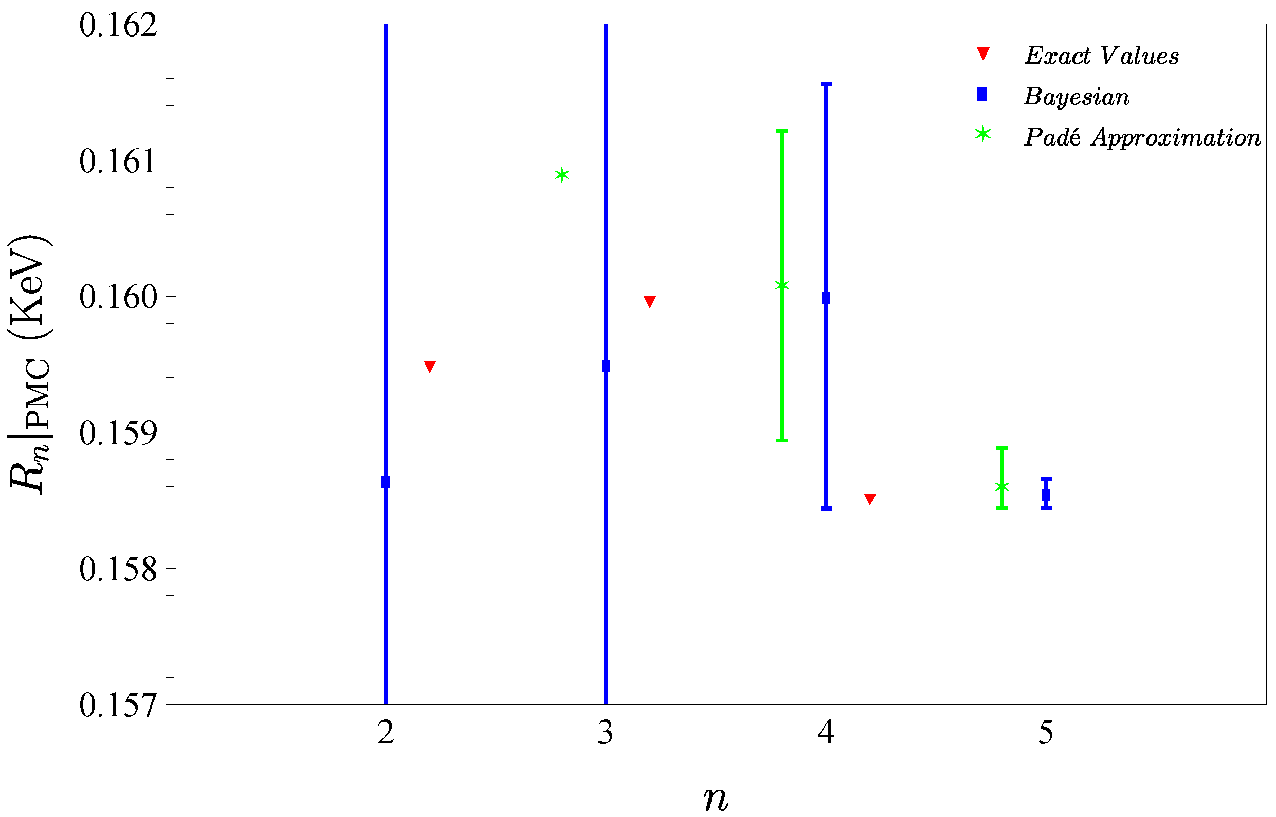
2.1. Basic Numerical Results and Discussions

To perform the numerical calculation, we took the values of the input parameters from the Particle Data Group [6], e.g., the W-boson mass $M_W$ = 80.377 GeV, the $\tau$-lepton mass $M_{\tau }$ = 1.7769 GeV, the b-quark pole mass $M_b$ = 4.78 GeV, the c-quark pole mass $M_c$ = 1.67 GeV, the t-quark pole mass $M_t$ = 172.69 GeV, and the Higgs mass $M_H$ = 125.25 GeV. The Fermi constant was $G_F=1.1664\times {10}^{-5}{\mathrm{GeV}}^{-2}$ and the fine-structure constant was $\alpha$ = 1/137.036. We assumed the running of ${\alpha }_s$ was at the four-loop level; the QCD asymptotic scale ${\Lambda }_{\mathrm{QCD}}$ was determined by using ${\alpha }_s\left(M_Z\right)=0.1179$, which gave ${\Lambda }_{\mathrm{QCD}}^{n_f=5}=0.2072$ GeV.

For the process $H\to \gamma \gamma$, its QCD correction $R_n$ under the $\overline{\mathrm{MS}}$-scheme was calculated up to the N⁴LO level. The initial fixed-order pQCD series was scheme-and-scale-dependent. (A way of achieving a scheme-and-scale-invariant prediction directly from the initial series, which is called the principle of minimum sensitivity (PMS), has been suggested in the literature. It assumes that all uncalculated higher-order terms give zero contribution and determines the optimal scheme and scale by requiring the slope of the pQCD series over the scheme-and-scale choices vanish. Since the PMS breaks the standard renormalization group invariance [45], it cannot be treated as a strict solution of conventional scheme-and-scale ambiguities, which, however, could be treated as an effective treatment.) As has been discussed above, after applying the PMC, the resultant conformal series becomes scheme-and-scale-invariant. We present the scale-invariant conformal coefficients ${\widehat{r}}_{i,0}(i=1,\dots ,4)$ in

Table 1. The $\overline{\mathrm{MS}}$ coefficients ${\widehat{r}}_{i,0}$ and $r_i$ for $R_4$. The coefficients $r_i$ are also scale-dependent, and their values under three typical scale choices, e.g., ${\mu }_r=M_H/2$, $M_H$, and $2M_H$, are given for comparison.

	$\mathit{i}=1$	$\mathit{i}=2$	$\mathit{i}=3$	$\mathit{i}=4$
$r_i({\mu }_r=M_H/2)$	$1.4070$	$-0.9874$	$-0.4084$	$3.3437$
$r_i({\mu }_r=M_H)$	$1.4070$	$0.2024$	$-1.6545$	$-0.3693$
$r_i({\mu }_r=2M_H)$	$1.4070$	$1.5282$	$-0.3456$	$-2.4065$
${\widehat{r}}_{i,0}$	$1.4070$	$1.3387$	$-3.6304$	$4.5695$

, where the scale-dependent coefficients $r_i$ at ${\mu }_r=M_H/2$, $M_H$ and $2M_H$ are also presented for comparison.

Using the expansion coefficients of the QCD corrections $R_2$, $R_3$, and $R_4$, the PMC scale can be fixed at the LL accuracy, NLL accuracy and N²LL accuracy, respectively, and we obtain

$$\begin{array}{ccc}\hfill Q_{\ast ,\mathrm{LL}}& =& 242.791\mathrm{GeV},\hfill \end{array}$$

(20)

$$\begin{array}{ccc}\hfill Q_{\ast ,\mathrm{NLL}}& =& 193.457\mathrm{GeV},\hfill \end{array}$$

(21)

$$\begin{array}{ccc}\hfill Q_{\ast ,{\mathrm{N}}^2\mathrm{LL}}& =& 213.603\mathrm{GeV}.\hfill \end{array}$$

(22)

$|Q_{\ast ,{\mathrm{N}}^2\mathrm{LL}}-Q_{\ast ,\mathrm{NLL}}\left|<\right|Q_{\ast ,\mathrm{NLL}}-Q_{\ast ,\mathrm{LL}}|$ indicates that the expansion series of $ln{Q}_{\ast }^2/Q^2$ has a perturbative nature. Together with the fact that its higher-order terms will suffer from both ${\alpha }_s$-power suppression and exponential suppression, the residual scale dependence of $Q_{\ast }$ due to even higher-order terms of $R_n$ will be highly suppressed, whose effects on the magnitude of ${\alpha }_s$ is negligible. The PMC predictions of $R_2$, $R_3$, and $R_4$ are

$$\begin{array}{ccc}\hfill R_2{|}_{\mathrm{PMC}}& =& 0.159493\mathrm{keV},\hfill \end{array}$$

(23)

$$\begin{array}{ccc}\hfill R_3{|}_{\mathrm{PMC}}& =& 0.159969\mathrm{keV},\hfill \end{array}$$

(24)

$$\begin{array}{ccc}\hfill R_4{|}_{\mathrm{PMC}}& =& 0.158517\mathrm{keV}.\hfill \end{array}$$

(25)

Table 2. The N⁴LO QCD corrections $R_4={\sum }_{i=1}^4{\Delta }_i$ of $\Gamma (H\to \gamma \gamma )$ under conventional (Conv.) and PMC scale settings, respectively. ${\Delta }_i$ represents the individual decay width at the NLO, N²LO, N³LO or N⁴LO level, respectively. Three typical values ${\mu }_r=M_H/2$, $M_H$, and $2M_H$ are adopted to show the renormalization scale uncertainty.

		$\mathit{i}=1$	$\mathit{i}=2$	$\mathit{i}=3$	$\mathit{i}=4$	${\mathit{R}}_4\left({\mathit{\mu }}_{\mathit{r}}\right)$
	${\mu }_r=M_H/2$	$0.17589$	$-0.01543$	$-0.00080$	$0.00082$	$0.16048$
${\Delta }_i\left(\mathrm{KeV}\right){|}_{\mathrm{Conv}.}$	${\mu }_r=M_H$	$0.15830$	$0.00256$	$-0.00236$	$-0.00006$	$0.15845$
	${\mu }_r=2M_H$	$0.14467$	$0.01616$	$-0.00038$	$-0.00027$	$0.16018$
${\Delta }_i\left(\mathrm{KeV}\right){|}_{\mathrm{PMC}}$	${\mu }_r\in [Q/2,2Q]$	$0.14744$	$0.01470$	$-0.00418$	$0.00055$	$0.15852$

shows the N⁴LO QCD corrections $R_4={\sum }_{i=1}^4{\Delta }_i$ under conventional and PMC scale settings, where ${\Delta }_i$ represents the individual decay width at the NLO, the N²LO, the N³LO or the N⁴LO level, respectively. Three typical scales ${\mu }_r=M_H/2$, $M_H$, and $2M_H$ were adopted to show the conventional renormalization scale uncertainty. Table 2 shows that under conventional scale setting, the separate decay widths ${\Delta }_i$ are highly scale-dependent, and due to the large cancellation among different orders, the net scale dependence of the N⁴LO prediction $R_4$ becomes small $\sim 1.28\%$ for ${\mu }_r\in [M_H/2,2M_H]$. After applying the PMC, both ${\Delta }_i$ and $R_4$ are scale-independent. This confirms the observation that if the correct magnitude of ${\alpha }_s$ of a pQCD series has been determined by using the RG-involved $\left\{{\beta }_i\right\}$-terms, indicating a good match of ${\alpha }_s$ with its expansion coefficients, one will achieve a precise scale-independent pQCD prediction. Such scale-independent nature of the pQCD approximation can be treated as its intrinsic perturbative property. Due to the good perturbative nature of the PMC series of $R_n$, the difference between the magnitudes of $R_n$ and $R_{n-1}$ becomes smaller with the increment of the given loop numbers.

Under the Bayesian approach, we predicted the magnitude of the unknown coefficient $c_{i+1}$ from the known ones $\{c_1,\dots ,c_i\}$ with $c_i\to r_i$ (${\widehat{r}}_{i,0}$) for conventional (PMC) series, respectively. Our results are listed in

Table 3. The predicted smallest 95.5% CIs for the scale-dependent conventional coefficients $r_i\left({\mu }_r\right)$ at the scale ${\mu }_r=M_H$ and the scale-invariant coefficients ${\widehat{r}}_{i,0}(i=3,4,5)$ of $R_n({\mu }_r=M_H)$ via the Bayesian approach, where $M_H=125.25\mathrm{GeV}$. The values from given series (“ECs”) are presented for comparison.

	$r_2\left(M_H\right)$	$r_3\left(M_H\right)$	$r_4\left(M_H\right)$	$r_5\left(M_H\right)$
CI	$[-15.6334,15.6334]$	$[-3.8294,3.8294]$	$[-2.9303,2.9303]$	$[-2.4023,2.4023]$
EC	$0.2024$	$-1.6545$	$-0.3693$	−
	${\widehat{r}}_{2,0}$	${\widehat{r}}_{3,0}$	${\widehat{r}}_{4,0}$	${\widehat{r}}_{5,0}$
CI	$[-15.6334,15.6334]$	$[-3.8294,3.8294]$	$[-6.4298,6.4298]$	$[-6.6348,6.6348]$
EC	$1.3387$	$-3.6304$	$4.5695$	−

. From Table 1 and Table 3, we can see that the exact values of $r_{i,0}(i=2,3,4,)$ and $r_i(i=2,3,4)$ lay within the predicted 95.5% CIs. Moreover, we obtained the smallest 95.5% credible intervals (CIs) for the perturbative coefficients $r_5({\mu }_r=M_H)$ and $r_{5,0}$, which were $r_5\in [-2.4023,2.4023]$ and $r_{5,0}\in [-6.6348,6.6348]$, respectively. The values from given series (“ECs”) are presented for comparison.

Using the estimated $r_5\left(M_H\right)$ and ${\widehat{r}}_{5,0}$, the error of ${\Gamma }_{\mathrm{H}}$ caused by the UHO-terms for conventional series and PMC series under the Bayesian approach (B.A.) were

$$\begin{array}{cc}\hfill & \Delta {\Gamma }_H{|}_{\mathrm{Conv}.}^{\mathrm{UHO}}=\pm 8.523\times {10}^{-5}\mathrm{keV},\hfill \end{array}$$

(26)

$$\begin{array}{cc}\hfill & \Delta {\Gamma }_H{|}_{\mathrm{PMC}}^{\mathrm{UHO}}=\pm 1.65\times {10}^{-4}\mathrm{keV}.\hfill \end{array}$$

(27)

By further taking ${\mu }_r\in [M_H/2,2M_H]$, the conventional series also had the following scale uncertainty

$$\begin{array}{c}\hfill \Delta {\Gamma }_H{|}_{\mathrm{Conv}.}^{{\mu }_r}={(}_{-1.02\times {10}^{-5}}^{+2.03\times {10}^{-3}})\mathrm{keV}.\end{array}$$

(28)

Then, as a combination, the net errors caused by the N⁵LO UHO terms in conventional and PMC series were

$$\begin{array}{cc}\hfill & \Delta {\Gamma }_H{|}_{\mathrm{Conv}.}={(}_{-8.58\times {10}^{-5}}^{+2.03\times {10}^{-3}})\mathrm{keV}\hfill \end{array}$$

(29)

$$\begin{array}{cc}\hfill & \Delta {\Gamma }_H{|}_{\mathrm{PMC}}=\pm 1.65\times {10}^{-4}\mathrm{keV}\hfill \end{array}$$

(30)

where ${\mu }_r\in [M_H/2,2M_H]$.

In addition, for the more precise PMC series, we also adopted another usual way of estimating UHO contributions, e.g., the Padé approximation approach (PAA) [58,59,60] to estimate the UHO terms of $R_{\mathrm{n}}$. The PAA works when we know enough higher orders, e.g., $n\ge 2$ for the present case. The PAA has an intrinsic error due to the existence of different types of generating functions [61], and we took the result of the $[0/n-1]$ type as its central value and the results of other types were treated as its uncertainty. More explicitly, to estimate the N³LO magnitude from the given N²LO series, we used the $[0/1]$-type generating function; to estimate the N⁴LO magnitude from the given N³LO series, we used the $[0/2]$-type and $[1/1]$-type generating functions; to estimate the N⁵LO magnitude from the given N⁴LO series, we used the $[0/3]$-type, $[1/2]$-type, and $[2/1]$-type generating functions, etc. We put the results in Figure 1, where the “Exact Values” together with the Bayesian approach (B.A.) and Padé approximation approach (PAA) ones are presented. Figure 1 shows that for the B.A. approach, the “exact” value are always within the predicted error band, the predicted one-order-higher UHO error band is always within the predicted one-order-lower UHO error band, and the predicted UHO values become more accurate when more loop terms are known. Thus, if one has enough higher-order information to tame the probability density function, one may determine the precise contribution of the UHO terms. For the PAA, the “exact” N⁴LO value is outside of the predicted error bar, and the predicted N⁵LO error bar becomes better and is consistent with the B.A. one. In this sense, at least for the present case, the B.A. approach is more effective than the PAA.

From Equation (2), there are other error sources such as $\Delta M_H$, $\Delta m_t$ and $\Delta {\alpha }_s\left(M_Z\right)$ for the total decay width $\Gamma (H\to \gamma \gamma )$. For this purpose, we took $\Delta M_H=\pm 0.17$ GeV, $\Delta m_t=\pm 0.30$ GeV, and $\Delta {\alpha }_s\left(M_z\right)=\pm 0.0009$ GeV [6] to show their effects. When discussing the error caused by one parameter, the other parameters were fixed as their center values. Thus, we had

$$\begin{array}{cc}\hfill & \Delta {\Gamma }_H{|}_{\mathrm{Conv}.}^{\Delta M_H}={(}_{-5.423\times {10}^{-2}}^{+5.455\times {10}^{-2}})\mathrm{keV},\hfill \end{array}$$

(31)

$$\begin{array}{cc}\hfill & \Delta {\Gamma }_H{|}_{\mathrm{PMC}}^{\Delta M_H}={(}_{-5.421\times {10}^{-2}}^{+5.453\times {10}^{-2}})\mathrm{keV},\hfill \end{array}$$

(32)

$$\begin{array}{cc}\hfill & \Delta {\Gamma }_H{|}_{\mathrm{Conv}.}^{\Delta m_t}={(}_{-7.040\times {10}^{-4}}^{+6.999\times {10}^{-4}})\mathrm{keV},\hfill \end{array}$$

(33)

$$\begin{array}{cc}\hfill & \Delta {\Gamma }_H{|}_{\mathrm{PMC}}^{\Delta m_t}={(}_{-7.045\times {10}^{-4}}^{+7.004\times {10}^{-4}})\mathrm{keV},\hfill \end{array}$$

(34)

$$\begin{array}{cc}\hfill & \Delta {\Gamma }_H{|}_{\mathrm{Conv}.}^{\Delta {\alpha }_s\left(M_Z\right)}={(}_{-1.072\times {10}^{-3}}^{+1.071\times {10}^{-3}})\mathrm{keV},\hfill \end{array}$$

(35)

$$\begin{array}{cc}\hfill & \Delta {\Gamma }_H{|}_{\mathrm{PMC}}^{\Delta {\alpha }_s\left(M_Z\right)}={(}_{-1.062\times {10}^{-3}}^{+1.061\times {10}^{-3}})\mathrm{keV}.\hfill \end{array}$$

(36)

By adding all the mentioned errors in quadrature, our final results for the total decay ${\Gamma }_H$ of $H\to \gamma \gamma$ using the B.A. approach were

$$\begin{array}{cc}\hfill & {\Gamma }_H{|}_{\mathrm{Conv}.}^{\mathrm{B}.\mathrm{A}.}=9.{56497}_{-0.05424}^{+0.05461}\mathrm{keV},\hfill \end{array}$$

(37)

$$\begin{array}{cc}\hfill & {\Gamma }_H{|}_{\mathrm{PMC}}^{\mathrm{B}.\mathrm{A}.}=9.{56504}_{-0.05422}^{+0.05455}\mathrm{keV}\hfill \end{array}$$

(38)

whose net errors were $1.138\%$ and $1.137\%$. This shows that since the QCD correction was calculated up to the N⁴LO level, the main errors were dominated by $\Delta M_H$. (As a rough estimation, by setting all input parameters to be their central values, the magnitudes of the EW or the QCD-EW mixing correction are $\sim \mathcal{O}(-2.1\times {10}^{-1}\mathrm{keV})$ or $\sim \mathcal{O}(+1.6\times {10}^{-1}\mathrm{keV})$, and then the errors caused by one-order-higher EW or QCD-EW corrections should be $\sim \mathcal{O}(-1.5\times {10}^{-3}\mathrm{keV})$ or $\sim \mathcal{O}(+1.2\times {10}^{-3}\mathrm{keV})$ because of the $\alpha$ suppression. Furthermore, due to different sign of the EW and QCD-EW mixing corrections, their net error becomes $\sim \mathcal{O}(3.0\times {10}^{-4}\mathrm{keV})$. Those magnitudes are also smaller than the dominant error caused by $\Delta M_H$.)

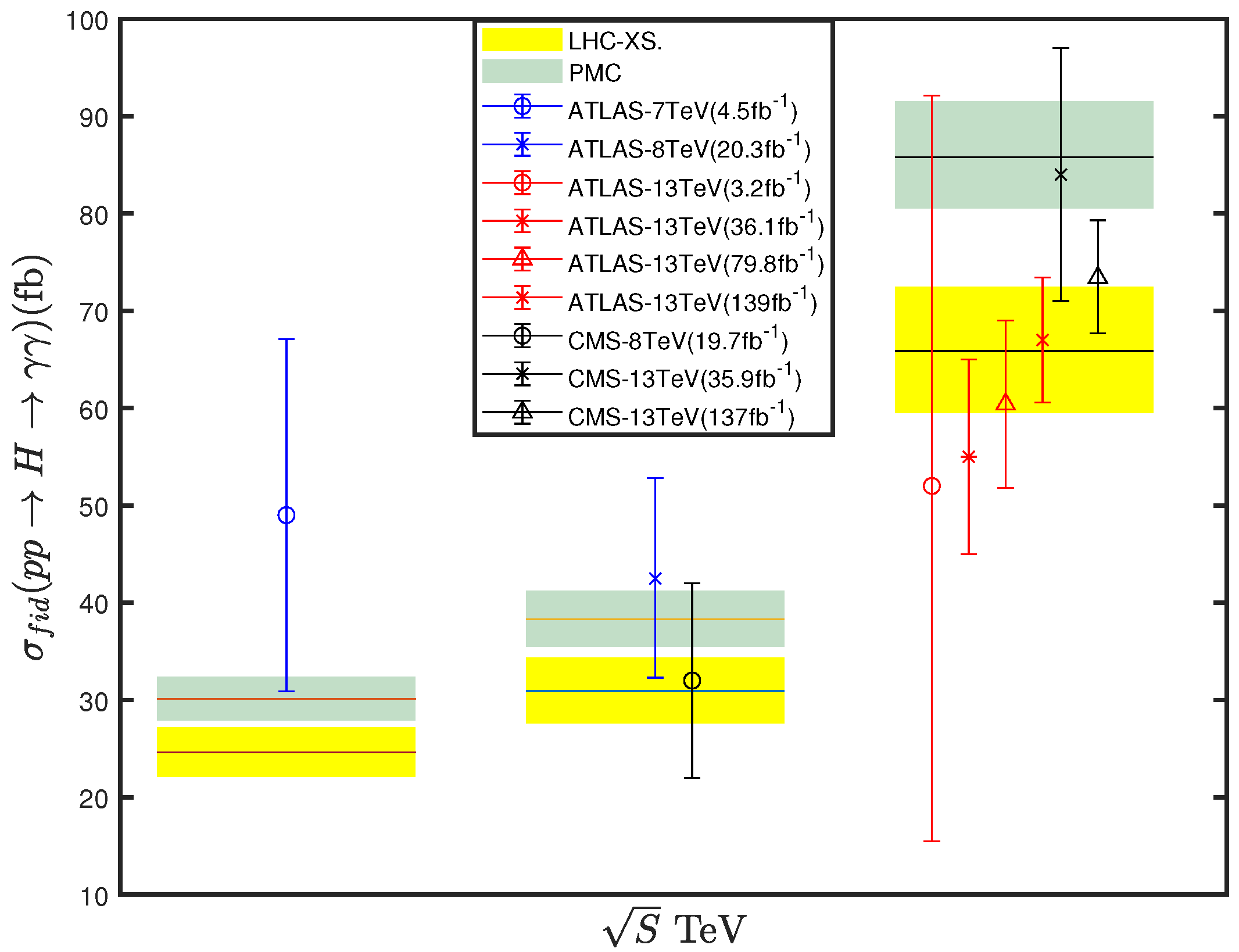
2.2. The Fiducial Cross Section of ${\sigma }_{\mathrm{fid}}(pp\to H\to \gamma \gamma )$

As an application of the $H\to \gamma \gamma$ decay width, we estimated the “fiducial cross section” of the process $pp\to H\to \gamma \gamma$. The fiducial cross section ${\sigma }_{\mathrm{fid}}$ can be written as

$$\begin{array}{c}\hfill {\sigma }_{\mathrm{fid}}(pp\to H\to \gamma \gamma )={\sigma }_{\mathrm{Incl}}{\mathcal{B}}_{H\to \gamma \gamma }A\end{array}$$

(39)

where A is the acceptance factor, whose value for different collision energies can be found in Ref. [62]. $B_{H\to \gamma \gamma }$ represents the branching ratio of $H\to \gamma \gamma$. By using $\Gamma (H\to \gamma \gamma )$ with a conventional-scale-setting approach, the LHC-XS group gave ${\mathcal{B}}_{H\to \gamma \gamma }=0.{00227}_{-0.00208}^{+0.00206}$ [63]. The inclusive cross section ${\sigma }_{\mathrm{Incl}}$ predicted by the LHC-XS group is given in Ref. [64]. The results are ${\sigma }_{\mathrm{fid}}{(pp\to H\to \gamma \gamma )|}_{\mathrm{LHC}-\mathrm{XS}}=24.{63}_{-2.50}^{+2.55}$ fb, $30.{93}_{-3.33}^{+3.44}$ fb, and $65.{86}_{-6.33}^{+6.58}$ fb for the proton–proton center-of-mass collision energy $\sqrt{\mathrm{S}}$ = 7, 8, and 13 TeV, respectively, which has been measured by the ATLAS and CMS collaborations with increasing integrated luminosities [62,65,66,67,68,69,70]. Taking the same inputs as those of Refs. [63,64,71], e.g., $M_H$ = 125 GeV and $M_t$ = 173.3 GeV, and using the QCD corrections up to the N⁴LO level, we obtained ${\sigma }_{\mathrm{fid}}{(pp\to H\to \gamma \gamma )|}_{\mathrm{PMC}}=30.1_{-2.2}^{+2.3}$ fb, $38.3_{-2.8}^{+2.9}$ fb, and $85.5_{-5.3}^{+5.7}$ fb for the proton–proton center-of-mass collision energy $\sqrt{\mathrm{S}}$ = 7, 8, and 13 TeV, respectively. As an intuitive comparison of the experimental data and theoretical results, we present the results in Figure 2 (Due to the resummation of the given $\left\{{\beta }_i\right\}$-type terms, which determine the precise magnitudes of ${\alpha }_s$ at different proton–proton center-of-mass collision energies, the PMC predictions are always larger than the LHC-XS predictions using conventional series.). It shows that when $\sqrt{\mathrm{S}}$ = 7 or 8 TeV, the theoretical results are consistent with the experimental measurements, and when $\sqrt{\mathrm{S}}$ = 13 TeV, the measured values of ATLAS and CMS differ significantly, and the theoretical results are closer to the data of CMS.

3. Summary

By using the PMC-scale-setting approaches, all nonconformal terms were adopted to set the correct magnitude of ${\alpha }_s$ with the help of the RGE, and the resultant pQCD series became more precise without the conventional scheme-and-scale independence. In this paper, we calculated the decay width $\Gamma (H\to \gamma \gamma )$ up to the N⁴LO QCD corrections. A Bayesian approach was applied to estimate the uncalculated N⁵LO contribution, which was only about $\pm 1.65\times {10}^{-4}$ keV for the case of the smallest $95.5\%$ credible interval. After taking all the mentioned errors into consideration, we predicted ${\Gamma }_H{|}_{\mathrm{PMC}}^{\mathrm{B}.\mathrm{A}.}=9.{56504}_{-0.05422}^{+0.05455}$ keV. Thus, by using the Bayesian approach, one can consistently obtain high-reliability estimations of UHO contributions by using convergent and scale-independent PMC series, greatly improving the prediction ability of pQCD.

References

1. Aad, G.; Abajyan, T.; Abbott, B.; Abdallah, J.; Khalek, S.A.; Abdelalim, A.A.; Aben, R.; Abi, B.; Abolins, M.; AbouZeid, O.S.; et al. Observation of a new particle in the search for the Standard Model Higgs boson with the ATLAS detector at the LHC. Phys. Lett. B 2012, 716, 1–29. [Google Scholar] [CrossRef]
2. Chatrchyan, S.; Khachatryan, V.; Sirunyan, A.M.; Tumasyan, A.; Adam, W.; Aguilo, E.; Bergauer, T.; Dragicevic, M.; Erö, J.; Fabjan, C.; et al. Observation of a New Boson at a Mass of 125 GeV with the CMS Experiment at the LHC. Phys. Lett. B 2012, 716, 30–61. [Google Scholar] [CrossRef]
3. Baer, H.; Barklow, T.; Fujii, K.; Gao, Y.; Hoang, A.; Kanemura, S.; List, J.; Logan, H.E.; Nomerotski, A.; Perelstein, M.; et al. The International Linear Collider Technical Design Report—Volume 2: Physics. arXiv 2013, arXiv:1306.6352. [Google Scholar]
4. Guimaraes da Costa, J.B.; Gao, Y.; Jin, S.; Qian, J.; Tully, C.G.; Young, C.; Wang, L.T.; Ruan, M.; Zhu, H.; Dong, M. CEPC Conceptual Design Report: Volume 2—Physics & Detector. arXiv 2018, arXiv:1811.10545. [Google Scholar]
5. Abada, A.; Abbrescia, M.; AbdusSalam, S.S.; Abdyukhanov, I.; Abelleira Fernandez, J.; Abramov, A.; Aburaia, M.; Acar, A.O.; Adzic, P.R.; Agrawal, P.; et al. FCC Physics Opportunities: Future Circular Collider Conceptual Design Report Volume 1. Eur. Phys. J. C 2019, 79, 474. [Google Scholar] [CrossRef]
6. Data Group; Workman, R.L.; Burkert, V.D.; Crede, V.; Klempt, E.; Thoma, U.; Tiator, L.; Agashe, K.; Aielli, G.; Allanach, B.C.; et al. Review of Particle Physics. Prog. Theor. Exp. Phys. 2022, 2022, 083C01. [Google Scholar]
7. Yu, Q.; Wu, X.G.; Wang, S.Q.; Huang, X.D.; Shen, J.M.; Zeng, J. Properties of the decay Hγγ using the approximate α s 4 corrections and the principle of maximum conformality. Chin. Phys. C 2019, 43, 093102. [Google Scholar] [CrossRef]
8. Ellis, J.R.; Gaillard, M.K.; Nanopoulos, D.V. A Phenomenological Profile of the Higgs Boson. Nucl. Phys. B 1976, 106, 292. [Google Scholar] [CrossRef]
9. Shifman, M.A.; Vainshtein, A.I.; Voloshin, M.B.; Zakharov, V.I. Low-Energy Theorems for Higgs Boson Couplings to Photons. Sov. J. Nucl. Phys. 1979, 30, 711. [Google Scholar]
10. Zheng, H.Q.; Wu, D.D. First order QCD corrections to the decay of the Higgs boson into two photons. Phys. Rev. D 1990, 42, 3760. [Google Scholar] [CrossRef]
11. Dawson, S.; Kauffman, R.P. QCD corrections to Hγγ. Phys. Rev. D 1993, 47, 1264. [Google Scholar] [CrossRef]
12. Djouadi, A.; Spira, M.; van der Bij, J.J.; Zerwas, P.M. QCD corrections to gamma gamma decays of Higgs particles in the intermediate mass range. Phys. Lett. B 1991, 257, 187. [Google Scholar] [CrossRef]
13. Djouadi, A.; Spira, M.; Zerwas, P.M. Two photon decay widths of Higgs particles. Phys. Lett. B 1993, 311, 255. [Google Scholar] [CrossRef]
14. Melnikov, K.; Yakovlev, O.I. Higgs → two photon decay: QCD radiative correction. Phys. Lett. B 1993, 312, 179. [Google Scholar] [CrossRef]
15. Inoue, M.; Najima, R.; Oka, T.; Saito, J. QCD corrections to two photon decay of the Higgs boson and its reverse process. Mod. Phys. Lett. A 1994, 9, 1189. [Google Scholar] [CrossRef]
16. Spira, M.; Djouadi, A.; Graudenz, D.; Zerwas, P.M. Higgs boson production at the LHC. Nucl. Phys. B 1995, 453, 17. [Google Scholar] [CrossRef]
17. Fleischer, J.; Tarasov, O.V.; Tarasov, V.O. Analytical result for the two loop QCD correction to the decay H→2γ. Phys. Lett. B 2004, 584, 294. [Google Scholar] [CrossRef]
18. Harlander, R.; Kant, P. Higgs production and decay: Analytic results at next-to-leading order QCD. J. High Energy Phys. 2005, 12, 015. [Google Scholar] [CrossRef]
19. Anastasiou, C.; Buehler, S.; Herzog, F.; Lazopoulos, A. Inclusive Higgs boson cross-section for the LHC at 8 TeV. J. High Energy Phys. 2012, 2012, 4. [Google Scholar] [CrossRef]
20. Maierhöfer, P.; Marquard, P. Complete three-loop QCD corrections to the decay H→γγ. Phys. Lett. B 2013, 721, 131. [Google Scholar] [CrossRef]
21. Sturm, C. Higher order QCD results for the fermionic contributions of the Higgs-boson decay into two photons and the decoupling function for the MS ¯ renormalized fine-structure constant. Eur. Phys. J. C 2014, 74, 2978. [Google Scholar] [CrossRef]
22. Marquard, P.; Smirnov, A.V.; Smirnov, V.A.; Steinhauser, M.; Wellmann, D. MS ¯ -on-shell quark mass relation up to four loops in QCD and a general SU(N) gauge group. Phys. Rev. D 2016, 94, 074025. [Google Scholar] [CrossRef]
23. Davies, J.; Herren, F. Higgs boson decay into photons at four loops. Phys. Rev. D 2021, 104, 053010. [Google Scholar] [CrossRef]
24. Actis, S.; Passarino, G.; Sturm, C.; Uccirati, S. NNLO Computational Techniques: The Cases Hγγ and Hgg. Nucl. Phys. B 2009, 811, 182. [Google Scholar] [CrossRef]
25. Benedikt, M.; Mertens, V.; Cerutti, F.; Riegler, W.; Otto, T.; Tommasini, D.; Tavian, L.J.; Gutleber, J.; Zimmermann, F.; Mangano, M.; et al. FCC-hh: The Hadron Collider: Future Circular Collider Conceptual Design Report Volume 3. Eur. Phys. J. Spec. Top. 2019, 228, 755. [Google Scholar]
26. Gross, D.J.; Wilczek, F. Ultraviolet Behavior of Nonabelian Gauge Theories. Phys. Rev. Lett. 1973, 30, 1343. [Google Scholar] [CrossRef]
27. Politzer, H.D. Reliable Perturbative Results for Strong Interactions? Phys. Rev. Lett. 1973, 30, 1346. [Google Scholar] [CrossRef]
28. Caswell, W.E. Asymptotic Behavior of Nonabelian Gauge Theories to Two Loop Order. Phys. Rev. Lett. 1974, 33, 244. [Google Scholar] [CrossRef]
29. Jones, D.R.T. Two Loop Diagrams in Yang-Mills Theory. Nucl. Phys. B 1974, 75, 531. [Google Scholar] [CrossRef]
30. Tarasov, O.V.; Vladimirov, A.A.; Zharkov, A.Y. The Gell-Mann-Low Function of QCD in the Three Loop Approximation. Phys. Lett. B 1980, 93, 429. [Google Scholar] [CrossRef]
31. Larin, S.A.; Vermaseren, J.A.M. The Three loop QCD Beta function and anomalous dimensions. Phys. Lett. B 1993, 303, 334. [Google Scholar] [CrossRef]
32. van Ritbergen, T.; Vermaseren, J.A.M.; Larin, S.A. The Four loop beta function in quantum chromodynamics. Phys. Lett. B 1997, 400, 379. [Google Scholar] [CrossRef]
33. Chetyrkin, K.G. Four-loop renormalization of QCD: Full set of renormalization constants and anomalous dimensions. Nucl. Phys. B 2005, 710, 499. [Google Scholar] [CrossRef]
34. Czakon, M. The Four-loop QCD beta-function and anomalous dimensions. Nucl. Phys. B 2005, 710, 485. [Google Scholar] [CrossRef]
35. Baikov, P.A.; Chetyrkin, K.G.; Kühn, J.H. Five-Loop Running of the QCD running coupling constant. Phys. Rev. Lett. 2017, 118, 082002. [Google Scholar] [CrossRef]
36. Herzog, F.; Ruijl, B.; Ueda, T.; Vermaseren, J.A.M.; Vogt, A. The five-loop beta function of Yang-Mills theory with fermions. J. High Energy Phys. 2017, 2017, 90. [Google Scholar] [CrossRef]
37. Luthe, T.; Maier, A.; Marquard, P.; Schröder, Y. The five-loop Beta function for a general gauge group and anomalous dimensions beyond Feynman gauge. J. High Energy Phys. 2017, 2017, 166. [Google Scholar] [CrossRef]
38. Wang, S.Q.; Wu, X.G.; Zheng, X.C.; Shen, J.M.; Zhang, Q.L. The Higgs boson inclusive decay channels Hb b ¯ and Hgg up to four-loop level. Eur. Phys. J. C 2014, 74, 2825. [Google Scholar] [CrossRef]
39. Brodsky, S.J.; Wu, X.G. Scale Setting Using the Extended Renormalization Group and the Principle of Maximum Conformality: The QCD Coupling Constant at Four Loops. Phys. Rev. D 2012, 85, 034038. [Google Scholar] [CrossRef]
40. Brodsky, S.J.; Giustino, L.D. Setting the Renormalization Scale in QCD: The Principle of Maximum Conformality. Phys. Rev. D 2012, 86, 085026. [Google Scholar] [CrossRef]
41. Brodsky, S.J.; Wu, X.G. Application of the Principle of Maximum Conformality to Top-Pair Production. Phys. Rev. D 2012, 86, 014021. [Google Scholar] [CrossRef]
42. Mojaza, M.; Brodsky, S.J.; Wu, X.G. Systematic All-Orders Method to Eliminate Renormalization-Scale and Scheme Ambiguities in Perturbative QCD. Phys. Rev. Lett. 2013, 110, 192001. [Google Scholar] [CrossRef]
43. Brodsky, S.J.; Mojaza, M.; Wu, X.G. Systematic Scale-Setting to All Orders: The Principle of Maximum Conformality and Commensurate Scale Relations. Phys. Rev. D 2014, 89, 014027. [Google Scholar] [CrossRef]
44. Wu, X.G.; Brodsky, S.J.; Mojaza, M. The Renormalization Scale-Setting Problem in QCD. Prog. Part. Nucl. Phys. 2013, 72, 44. [Google Scholar] [CrossRef]
45. Wu, X.G.; Ma, Y.; Wang, S.Q.; Fu, H.B.; Ma, H.H.; Brodsky, S.J.; Mojaza, M. Renormalization Group Invariance and Optimal QCD Renormalization Scale-Setting. Rept. Prog. Phys. 2015, 78, 126201. [Google Scholar] [CrossRef]
46. Wu, X.G.; Shen, J.M.; Du, B.L.; Huang, X.D.; Wang, S.Q.; Brodsky, S.J. The QCD Renormalization Group Equation and the Elimination of Fixed-Order Scheme-and-Scale Ambiguities Using the Principle of Maximum Conformality. Prog. Part. Nucl. Phys. 2019, 108, 103706. [Google Scholar] [CrossRef]
47. Gell-Mann, M.; Low, F.E. Quantum electrodynamics at small distances. Phys. Rev. 1954, 95, 1300. [Google Scholar] [CrossRef]
48. Brodsky, S.J.; Lepage, G.P.; Mackenzie, P.B. On the Elimination of Scale Ambiguities in Perturbative Quantum Chromodynamics. Phys. Rev. D 1983, 28, 228. [Google Scholar] [CrossRef]
49. Shen, J.M.; Wu, X.G.; Du, B.L.; Brodsky, S.J. Novel All-Orders Single-Scale Approach to QCD Renormalization Scale-Setting. Phys. Rev. D 2017, 95, 094006. [Google Scholar] [CrossRef]
50. Stueckelberg de Breidenbach, E.C.G.; Petermann, A. Normalization of constants in the quanta theory. Helv. Phys. Acta 1953, 26, 499. [Google Scholar]
51. Peterman, A. Renormalization Group and the Deep Structure of the Proton. Phys. Rept. 1979, 53, 157. [Google Scholar] [CrossRef]
52. Wang, S.Q.; Wu, X.G.; Zheng, X.C.; Chen, G.; Shen, J.M. An analysis of Hγγ up to three-loop QCD corrections. J. Phys. G 2014, 41, 075010. [Google Scholar] [CrossRef]
53. Cacciari, M.; Houdeau, N. Meaningful characterization of perturbative theoretical uncertainties. J. High Energy Phys. 2011, 2011, 39. [Google Scholar] [CrossRef]
54. Bagnaschi, E.; Cacciari, M.; Guffanti, A.; Jenniches, L. An extensive survey of the estimation of uncertainties from missing higher orders in perturbative calculations. J. High Energy Phys. 2015, 2015, 133. [Google Scholar] [CrossRef]
55. Bonvini, M. Probabilistic definition of the perturbative theoretical uncertainty from missing higher orders. Eur. Phys. J. C 2020, 80, 989. [Google Scholar] [CrossRef]
56. Duhr, C.; Huss, A.; Mazeliauskas, A.; Szafron, R. An analysis of Bayesian estimates for missing higher orders in perturbative calculations. J. High Energy Phys. 2021, 2021, 122. [Google Scholar] [CrossRef]
57. Shen, J.M.; Zhou, Z.J.; Wang, S.Q.; Yan, J.; Wu, Z.F.; Wu, X.G.; Brodsky, S.J. Extending the Predictive Power of Perturbative QCD Using the Principle of Maximum Conformality and Bayesian Analysis. Eur. Phys. J. C 2023, 83, 326. [Google Scholar] [CrossRef]
58. Basdevant, J.L. The Pade approximation and its physical applications. Fortsch. Phys. 1972, 20, 283. [Google Scholar] [CrossRef]
59. Samuel, M.A.; Li, G.; Steinfelds, E. Estimating perturbative coefficients in quantum field theory using Pade approximants. 2. Phys. Lett. B 1994, 323, 188. [Google Scholar] [CrossRef]
60. Samuel, M.A.; Ellis, J.R.; Karliner, M. Comparison of the Pade approximation method to perturbative QCD calculations. Phys. Rev. Lett. 1995, 74, 4380. [Google Scholar] [CrossRef]
61. Du, B.L.; Wu, X.G.; Shen, J.M.; Brodsky, S.J. Extending the Predictive Power of Perturbative QCD. Eur. Phys. J. C 2019, 79, 182. [Google Scholar] [CrossRef]
62. Aad, G. et al. [ATLAS Collaboration] Measurement of the Higgs Boson Production cross Section at 7, 8 and 13 TeV Center-of-Mass Energies in the Hγγ Channel with the ATLAS Detector. ATLAS-CONF-2015-060. Available online: http://cds.cern.ch/record/2114826 (accessed on 1 September 2022).
63. de Florian, D.; Fontes, D.; Quevillon, J.; Schumacher, M.; Llanes-Estrada, F.J.; Gritsan, A.V.; Vryonidou, E.; Signer, A.; de Castro, M.P.; Pagani, D.; et al. Handbook of LHC Higgs Cross Sections: 4. Deciphering the Nature of the Higgs Sector. arXiv 2016, arXiv:1610.07922. [Google Scholar]
64. Heinemeyer, S.; Mariotti, C.; Passarino, G.; Tanaka, R.; Andersen, J.R.; Artoisenet, P.; Bagnaschi, E.A.; Banfi, A.; Becher, T.; Bernlochner, F.U.; et al. Handbook of LHC Higgs Cross Sections: 3. Higgs Properties. arXiv 2013, arXiv:1307.1347. [Google Scholar]
65. ATLAS. Measurements of Higgs Boson Properties in the Diphoton Decay Channel with 36.1 fb−1 pp Collision Data at the Center-of-Mass Energy of 13 TeV with the ATLAS Detector. ATLAS-CONF-2017-045. Available online: http://cds.cern.ch/record/2273852 (accessed on 1 September 2022).
66. ATLAS. Combination of Searches for Heavy Resonances Using 139 fb−1 of proton–proton Collision Data at s = 13 TeV with the ATLAS Detector. ATLAS-CONF-2022-028. Available online: http://cds.cern.ch/record/2809967 (accessed on 1 September 2022).
67. Alves, L.; Lucio, F. Fiducial and differential cross-section measurements in the di-photon channel using full Run2 dataset at ATLAS. In Proceedings of the 41st International Conference on High Energy Physics (ICHEP 2022), Bologna, Italy, 6–13 July 2022; p. 1051. [Google Scholar]
68. CMS. Measurement of Differential Fiducial Cross Sections for Higgs Boson Production in the Diphoton Decay Channel in pp Collisions at s = 13 TeV. CMS-PAS-HIG-17-015. Available online: http://cds.cern.ch/record/2257530 (accessed on 1 September 2022).
69. Khachatryan, V.; Sirunyan, A.M.; Tumasyan, A.; Adam, W.; Asilar, E.; Bergauer, T.; Brandstetter, J.; Brondolin, E.; Dragicevic, M.; Ero, J.; et al. Measurement of differential cross sections for Higgs boson production in the diphoton decay channel in pp collisions at s = 8 TeV. Eur. Phys. J. C 2016, 76, 13. [Google Scholar] [CrossRef] [PubMed]
70. Tumasyan, A.; Adam, W.; Andrejkovic, J.W.; Bergauer, T.; Chatterjee, S.; Damanakis, K.; Dragicevic, M.; Escalante Del Valle, A.; Hussain, P.S.; Jeitler, M.; et al. Measurement of the Higgs boson inclusive and differential fiducial production cross sections in the diphoton decay channel with pp collisions at s = 13 TeV. J. High Energy Phys. 2023, 2023, 091. [Google Scholar]
71. Wang, S.Q.; Wu, X.G.; Brodsky, S.J.; Mojaza, M. Application of the Principle of Maximum Conformality to the Hadroproduction of the Higgs Boson at the LHC. Phys. Rev. D 2016, 94, 053003. [Google Scholar] [CrossRef]
Figure 1. The predicted values for the pQCD correction R n | PMC under the Padé approximation approach (PAA) and Bayesian approach (B.A.) at different orders, respectively. The blue rectangles together with the error bars are for B.A., the green error bars are brought by different types of PAAs, and the exact values of the R n ( M H ) | PMC at different orders, respectively.
Symmetry 16 00173 g001
Figure 2. The fiducial cross section σ fid ( p p H γ γ ) using Γ ( H γ γ ) up to the N4LO level. The LHC−XS prediction, the ATLAS measurements [62,65,66,67], and the CMS measurement [68,69,70] are presented as a comparison.
Symmetry 16 00173 g002