
Canonical Construction of Invariant Differential Operators: A Review


Institute for Nuclear Research and Nuclear Energy, Bulgarian Academy of Sciences, 72 Tsarigradsko Chaussee, 1784 Sofia, Bulgaria
Symmetry 2024, 16(2), 151; https://doi.org/10.3390/sym16020151
Submission received: 3 November 2023
/
Revised: 3 December 2023
/
Accepted: 13 December 2023
/
Published: 27 January 2024
(This article belongs to the Section Physics)
Abstract
:In the present paper, we review the progress of the project of the classification and construction of invariant differential operators for non-compact, semisimple Lie groups. Our starting point is the class of algebras which we called earlier ‘conformal Lie algebras’ (CLA), which have very similar properties to the conformal algebras of Minkowski space-time, though our aim is to go beyond this class in a natural way. For this purpose, we introduced recently the new notion of a parabolic relation between two non-compact, semi-simple Lie algebras and that have the same complexification and possess maximal parabolic subalgebras with the same complexification.
1. Introduction and Preliminaries
Invariant differential operators play a very important role in the description of physical symmetries—starting from the early occurrences in the Maxwell, d’Allembert and Dirac, equations to the latest applications of (super)differential operators in conformal field theory, supergravity and string theory (for reviews, cf., e.g., [1,2]). Thus, it is important for applications in physics to systematically study such operators. For more relevant references cf., e.g., [3,4,5,6,7,8,9,10,11,12,13,14,15,16,17,18,19,20,21,22,23,24,25,26,27,28,29,30,31,32,33,34,35,36,37,38,39,40,41,42,43,44,45,46,47,48,49,50,51,52,53,54,55,56,57,58,59,60,61,62,63,64,65,66,67,68,69,70,71,72,73], and others throughout the text. Especially, we would like to point out the book [74] which contains a section devoted to groups of conformal transformations of curved spacetime.
In a recent paper [75], we started the systematic explicit construction of invariant differential operators. We gave an explicit description of the building blocks, namely, the parabolic subgroups and subalgebras from which the necessary representations are induced. Thus, we have set the stage for the study of different non-compact groups. Up to 2016, relevant references may be found in our monograph [76] and also in [77,78,79,80,81,82,83,84,85,86,87,88,89,90,91,92,93,94,95,96,97,98,99,100,101,102,103,104,105,106,107,108,109,110,111].
Our canonical construction is applicable also to quantum groups, super groups, to (super-)Virasoro and Kac-Moody algebras, see our monographs: [112,113,114].
Preliminaries
Let G be a semi-simple, non-compact Lie group, and K a maximal compact subgroup of G. Then, we have an Iwasawa decomposition , where is an Abelian simply connected vector subgroup of G and is a nilpotent simply connected subgroup of G preserved by the action of . Furthermore, let be the centralizer of in K. Then, the subgroup is a minimal parabolic subgroup of G. A parabolic subgroup is any subgroup of G which contains a minimal parabolic subgroup.
Furthermore let denote the Lie algebras of , resp.
For our purposes, we shall be restrict maximal parabolic subgroups , i.e., , resp., to maximal parabolic subalgebras with .
Let be a (non-unitary) character of A, , parameterized by a real number d, called the conformal weight or energy.
Furthermore, let fix a discrete series representation of M on the Hilbert space , or the finite-dimensional (non-unitary) representation of M with the same Casimirs.
We call the induced representation an elementary representation of G [24]. (These are called generalized principal series representations (or limits thereof) in [115].) Their spaces of functions are
where , , , . The representation action is the left regular action:
- An important ingredient in our considerations are the highest/lowest-weight representations of . These can be realized as (factor-modules of) Verma modules over , where , is a Cartan subalgebra of and weight is determined uniquely from [76].
Actually, since our ERs may be induced from finite-dimensional representations of (or their limits) the Verma modules are always reducible. Thus, it is more convenient to use generalized Verma modules such that the role of the highest/lowest-weight vector v0 is taken by the (finite-dimensional) space . For the generalized Verma modules (GVMs) the reducibility is controlled only by the value of the conformal weight d. Relatedly, for the intertwining differential operators, only the reducibility with regard to non-compact roots is essential.
- Another main ingredient of our approach is as follows. We group the (reducible) ERs with the same Casimirs in sets called multiplets [76]. The multiplet corresponding to fixed values of the Casimirs may be depicted as a connected graph, the vertices of which correspond to the reducible ERs and the lines (arrows) between the vertices correspond to intertwining operators. The explicit parameterization of the multiplets and of their ERs is important in understanding of the situation. The notion of multiplets was introduced in [116] and applied to representations of and , resp., induced from their minimal parabolic subalgebras. Then it was applied to the conformal superalgebra [117], to infinite-dimensional (super)algebras [113] and to quantum groups [112]. (For other applications, we refer to [114].)
In fact, the multiplets contain explicitly all the data necessary to construct the intertwining differential operators. Actually, the data for each intertwining differential operator consist of the pair , where is a (non-compact) positive root of , , such that the BGG Verma module reducibility condition (for highest-weight modules) is fulfilled:
where is half the sum of the positive roots of . When the above holds, then the Verma module with shifted weight (or for GVM and non-compact) is embedded in the Verma module (or ). This embedding is realized by a singular vector determined by a polynomial in the universal enveloping algebra , and is the subalgebra of generated by the negative root generators [118]. More explicitly, [76,119], (or for GVMs). Then, there exists [76,119] an intertwining differential operator
given explicitly by:
where denotes the right action on the functions .
In most of these situations, the invariant operator has a non-trivial invariant kernel in which a subrepresentation of is realized. Thus, studying the equations with trivial RHS is also very important:
For example, in many physical applications, in the case of first-order differential operators, i.e., for , these equations are called conservation laws, and the elements are called conserved currents.
The above construction also works for the subsingular vectors of Verma modules. Such vectors are also expressed by a polynomial in the universal enveloping algebra: , cf. [120]. Thus, there exists a conditionally invariant differential operator given explicitly by , and a conditionally invariant differential equation; for many more details, see [121]. (Note that these operators (equations) are not of the first order.)
In our exposition below, we shall use the so-called Dynkin labels:
where , is half the sum of the positive roots of .
We shall use also the so-called Harish–Chandra parameters:
where is any positive root of . These parameters are redundant, since they are expressed in terms of the Dynkin labels; however, some statements are best formulated in their terms. (Clearly, both the Dynkin labels and Harish–Chandra parameters have their origin in the BGG reducibility condition (3).)
Finally, we shall introduce the notion of ’parabolically related non-compact semisimple Lie algebras’ [122]. This notion is not part of our procedure for constructing invariant differential operators, but just a tool to extend the construction from one Lie algebra to another.
Definition 1.
Let be two non-compact semi-simple Lie algebras with the same complexification . We call them parabolically related if they have parabolic subalgebras , , such that ().♢
Certainly, there are many such parabolic relationships for any given algebra . Furthermore, two algebras may be parabolically related via different parabolic subalgebras.
The paper is organized as follows. In Section 2, we consider the case of the pseudo-orthogonal algebras which are parabolically related to the conformal algebra for . In Section 3, we consider the CLA and the parabolically related , and for : . In Section 4, we consider the CLA and—for —the parabolically related . In Section 5, we consider the algebras (which are CLA when n is even) and the parabolically related algebras. In Section 6, we consider the CLA and the parabolically related . In Section 7, we consider the hermitian symmetric case and the parabolically related and . In Section 8, we consider the algebra and its real forms and . In Section 9, we consider the algebra .
We would also like to list some more recent relevant references [123,124,125,126,127,128,129,130,131,132,133,134,135,136,137,138,139,140,141,142,143,144,145,146,147,148,149,150,151,152,153,154,155,156,157,158,159,160,161,162,163,164,165,166,167,168,169,170,171,172,173,174,175,176,177,178,179,180,181,182,183,184,185,186,187,188,189,190,191,192,193,194,195,196,197,198,199,200,201,202,203,204,205,206,207,208,209,210,211,212,213,214,215,216,217,218,219,220,221,222,223,224,225,226,227,228,229].
2. Conformal Algebras and Parabolically Related Algebras
The most widely used algebras are the conformal algebras in n-dimensional Minkowski space-time. In that case, there is a maximal Bruhat decomposition [230] that has direct physical meaning:
where is the Lorentz algebra of n-dimensional Minkowski space-time, the subalgebra represents the dilatations and the conjugated subalgebras , are the algebras of translations and special conformal transformations, both being isomorphic to n-dimensional Minkowski space-time.
Another physically important feature is that the algebras have discrete series representations. We recall that by the Harish–Chandra criterion [231], these are groups where the following holds:
where K is the maximal compact subgroup of the non-compact group G.
Furthermore, the algebras belong to the class of Hermitian symmetric spaces. The practical criterion is that in these cases, the maximal compact subalgebra is of the form:
The Lie algebras from this class are as follows:
These groups/algebras have highest/lowest-weight representations, and relatedly, holomorphic discrete series representations.
We label the signature of the ERs of as follows:
where the last entry of labels the characters of , and the first entries are labels of the finite-dimensional nonunitary irreps of .
The reason to use the parameter c instead of d is that the parametrization of the ERs in the multiplets is given in a simple intuitive way (cf. [232]):
Furthermore, we denote by the representation space with signature .
The number of ERs in the corresponding multiplets is equal to
where are Cartan subalgebras of , resp. This formula is valid for the main multiplets of all conformal Lie algebras.
The ERs in the multiplet are related by intertwining integral and differential operators. The integral operators were introduced by Knapp and Stein [233]. They correspond to elements of the restricted Weyl group of . These operators intertwine the pairs
The intertwining differential operators correspond to non-compact positive roots of the root system of , cf. [76]. (In the current context, compact roots of are those that are roots also of the subalgebra , the rest of the roots are non-compact.) The degrees of these intertwining differential operators are given just by the differences of the c entries [76]:
where is omitted from the first line for even.
Matters are arranged so that in every multiplet only the ER with signature contains a finite-dimensional nonunitary subrepresentation in a subspace . The latter corresponds to the finite-dimensional unitary irrep of with signature . The subspace is annihilated by the operator , and is the image of the operator .
- Interlude:
We mention one more special feature of , namely that the complexification of the maximal compact subgroup is isomorphic to the complexification of the first two factors of the Bruhat decomposition:
The coincidence of the complexification of the semi-simple subalgebras
means that the sets of finite-dimensional (nonunitary) representations of are in 1-to-1 correspondence with the finite-dimensional (unitary) representations of . The latter leads to the fact that the corresponding induced representations are representations of finite -type [234].
It turns out that some of the hermitian-symmetric algebras share the above-mentioned special properties of . This subclass consists of
with the corresponding analogs of Minkowski space-time V being
In view of applications to physics, we proposed to call these algebras ‘conformal Lie algebras’ (or groups).
We summarize the algebras parabolically related to conformal Lie algebras with maximal parabolics fulfilling (18) in Table 1 below. Also, some non-CLAs are included.
There, denotes as a real Lie algebra (thus, ); denotes the compact real form of ; and we have imposed restrictions to avoid coincidences or degeneracies due to well-known isomorphisms: , , , , , , .
Although the diagram in Figure 1 is valid for arbitrary (even ) due to the parabolic relatedness, the contents are very different. (The same remark holds for the diagram in Figure 2 valid for for odd .) We comment only on the ER with signature . In all cases, it contains a UIR of realized on an invariant subspace of the ER . That subspace is annihilated by the operator , and is the image of the operator . (Other ERs contain more UIRs.)
If , the mentioned UIR is a discrete series representation. (Other ERs contain more discrete series UIRs.)
And if , the invariant subspace is the direct sum of two subspaces , in which a holomorphic discrete series representation and its conjugate anti-holomorphic discrete series representation, resp., are realized. Note that the corresponding lowest-weight GVM is infinitesimally equivalent only to the holomorphic discrete series, while the conjugate highest-weight GVM is infinitesimally equivalent to the anti-holomorphic discrete series.
Note that , are Harish–Chandra parameters corresponding to the non-compact positive roots of . From these, only corresponds to a simple root; i.e., it is a Dynkin label.
Above, we considered for . The case is reduced to since . The case is special and must be treated separately. But, in fact, it is contained in what we presented already. In that case, the multiplets contain only two ERs which may be depicted by the top pair in the pictures that we presented. And they have the properties that we described for with . The case was given already in 1946-7 independently by Gel’fand et al. [235] and Bargmann [236].
3. The Lie Algebra and Parabolically Related Algebras
Let , . The maximal compact subgroup is , while . The number of ERs in the corresponding multiplets is equal to
The signature of the ERs of is
The Knapp–Stein restricted Weyl reflection is given by
Below, in Figure 3 and Figure 4, we give the diagrams for for [237]. (The case is already considered since .) These are also diagrams for the parabolically related , and for , these are also diagrams for the parabolically related [122].
We use the following conventions. Each intertwining differential operator is represented by an arrow accompanied by a symbol encoding the root and the number which is involved in the BGG criterion.
4. The Lie Algebras and (-even)
Let . Let be the split real form of . The maximal compact subgroup is , while . The number of ERs in the corresponding multiplets is
The signature of the ERs of is
The Knapp–Stein Weyl reflection acts as follows:
5. The Lie Algebra
The Lie algebra is given by
, .
The maximal compact subalgebra is . Thus, has discrete series representations and highest/lowest-weight representations. The split rank is .
The maximal parabolic subalgebras have -factors as follows [75]:
5.1. Case of
For even , we may choose a maximal parabolic such that , . We note also that
Thus, with this choice we utilize the property which distinguishes the class of ’conformal Lie algebras’ to which class the algebras belong.
Furthermore, we restrict ourselves to .
We label the signature of the ERs of as follows:
where the last entry of labels the characters of , and the first five entries are labels of the finite-dimensional (nonunitary) irreps of when all or limits of the latter when some .
Below, we shall use the following conjugation on the finite-dimensional entries of the signature:
The ERs in the multiplet are related also by intertwining integral operators introduced in [KnSt]. These operators are defined for any ER, the general action being:
Furthermore, we give the correspondence between the signatures and the highest weight . The connection is through the Dynkin labels:
where , is half the sum of the positive roots of . The explicit connection is
Finally, we recall that according to [75], the above considerations are applicable also for the algebra with parabolic -factor .
The main multiplets are in 1-to-1 correspondence with the finite-dimensional irreps of ; i.e., they are labeled by the six positive Dynkin labels .
The number of ERs/GVMs in the corresponding multiplets is [75]
where is a Cartan subalgebra of both and .
They are given explicitly in the Figure 9 below. The pairs are symmetric with regard to to the bullet in the middle of the figure—this represents the Weyl symmetry realized by the Knapp–Stein operators
The statements made for the ER with signature in the previous cases also remain valid here. Also, the conjugate ER contains a unitary discrete series subrepresentation split in highest/lowest-weight representations.
All the above is valid also for the algebra , cf. [75]; however, the latter algebra does not have highest/lowest-weight representations.
We present only the main multiplets. The reduced multiplets may be seen in [92].
5.2. Case of
This case was already considered for the choice of generic maximal parabolic subalgebra of , but here, we shall consider a Heisenberg maximal parabolic subalgebra.
We recall that has minimal parabolic:
The Satake–Dynkin diagram of is
![Symmetry 16 00151 i001]() where, by standard convention, the black dots represent the subalgebras of .
where, by standard convention, the black dots represent the subalgebras of .

We shall use the Heisenberg maximal parabolic (21) with -subalgebra:
The Satake–Dynkin diagram of is a subdiagram of (23)

From the above, it follows that the -compact roots of are (given in terms of the simple roots):
By definition, the above are the positive roots of .
The positive -noncompact roots of in terms of the simple roots are:
where, for convenience, we use the notation
To characterize the Verma modules, we shall first use the Dynkin labels:
where is half the sum of the positive roots of . Thus, we shall use:
Note that when all , then characterizes the finite-dimensional irreps of and its real forms, in particular, . Furthermore, characterizes the finite-dimensional irreps of the subalgebra.
For the -noncompact roots of , we shall also use the Harish–Chandra parameters:
and explicitly in terms of the Dynkin labels (compare (27)):
Main multiplets of SO*(8)
The main multiplets are in 1-to-1 correspondence with the finite-dimensional irreps of ; i.e., they are labeled by the four positive Dynkin labels .
We take . It has one embedded Verma module with HW . The number of ERs/GVMs in a main multiplet is 24. We give the whole multiplet as follows:
We shall label the signature of the ERs of also as follows:
where the last entry labels the characters of , and the first three entries of are labels of the finite-dimensional irreps of when all or limits of the latter when some . Note that is the Harish–Chandra parameter for the highest root .
Use of this labeling signatures may be given in the following pair-wise manner:
The ERs in the multiplet are alsonrelated by intertwining integral operators introduced in [233]. These operators are defined for any ER, the general action being:
The main multiplets are given explicitly in Figure 10. The pairs are symmetric with regard to to the dashed line in the middle the figure—this represents the Weyl symmetry realized by the Knapp–Stein operators .
Some comments are in order.
Matters are arranged so that in every multiplet only the ER with signature contains a finite-dimensional nonunitary subrepresentation in a finite-dimensional subspace . The latter corresponds to the finite-dimensional irrep of with signature . The subspace is annihilated by the operator , and is the image of the operator . The subspace is annihilated also by the intertwining differential operator acting from to . When all , then , and in that case, is also the trivial one-dimensional UIR of the whole algebra . Furthermore, in that case, the conformal weight is zero: .
In the conjugate ER , there is a unitary discrete series subrepresentation in an infinite-dimensional subspace with conformal weight . It is annihilated by the operator , and is the image of the operator .
Thus, for the ER with signature contains both a holomorphic discrete series representation and a conjugate anti-holomorphic discrete series representation. The direct sum of the holomorphic and the antiholomorphic representations spaces form the invariant subspace mentioned above. Note that the corresponding lowest-weight GVM is infinitesimally equivalent only to the holomorphic discrete series, while the conjugate highest-weight GVM is infinitesimally equivalent to the anti-holomorphic discrete series.
In Figure 10, we use the notation: . Each intertwining differential operator is represented by an arrow accompanied either by a symbol encoding the root and the number which is involved in the BGG criterion, or a symbol encoding the root and the number from BGG.
Finally, we recall that according to [122], the above considerations are applicable also for the algebra (with , ) with maximal Heisenberg parabolic subalgebra: , .
We present only the main multiplets. The reduced multiplets may be seen in [239].
5.3. Case of
The case is also special. It is not of the class of ‘conformal Lie algebras’ but belongs to the wider class of Hermitian symmetric spaces as described in the Introduction.
The maximal parabolic subalgebras of have -factors as follows [75]:
The factors in the maximal parabolic subalgebras have dimensions .
The case is special. In this case, we have a maximal Heisenberg parabolic with -factor
which we use in this section.
Furthermore, we restrict ourselves to our case of study with minimal parabolic:
The Satake–Dynkin diagram of is:
![Symmetry 16 00151 i003]() where, by standard convention, the black dots represent the subalgebras of and the left-right arrow represents the subalgebra of .
where, by standard convention, the black dots represent the subalgebras of and the left-right arrow represents the subalgebra of .

We shall use the Heisenberg maximal parabolic (37) with -subalgebra:
The Satake–Dynkin diagram of is a subdiagram of (40)
![Symmetry 16 00151 i004]() where the single black dot represents the subalgebra, while the connected part of the diagram represents the subalgebra.
where the single black dot represents the subalgebra, while the connected part of the diagram represents the subalgebra.

From the above follows that the -compact roots of are (given in terms of the simple roots):
By definition, the above are the positive roots of , namely: (43a) and (43b).
The positive -noncompact roots of in terms of the simple roots are
where, for convenience, we use the notation
To characterize the Verma modules, we shall use first the Dynkin labels:
where is half the sum of the positive roots of . Thus, we shall use:
Note that when all , then characterizes the finite-dimensional irreps of and its real forms, in particular, . Furthermore, characterizes the finite-dimensional irreps of the subalgebra, while the set of positive integers characterizes the finite-dimensional irreps of .
For the -noncompact roots of , we shall also use the Harish–Chandra parameters:
and explicitly in terms of the Dynkin labels (compare (44)):
Main multiplets of SO*(10)
The main multiplets are in 1-to-1 correspondence with the finite-dimensional irreps of ; i.e., they are labeled by the five positive Dynkin labels .
We take . It has one embedded Verma module with HW . The number of ERs/GVMs in a main multiplet is 40. We give the whole multiplet as follows:
We shall label the signature of the ERs of also as follows:
where the first entry labels the finite-dimensional irreps of , the second entry labels the characters of , the last three entries of are labels of the finite-dimensional (nonunitary) irreps of when all or limits of the latter when some . Note that is the Harish–Chandra parameter for the highest root .
Using this labeling, signatures may be given in the following pair-wise manner:
The ERs in the multiplet are also related by intertwining integral operators introduced in [233]. These operators are defined for any ER, the general action being:
The main multiplets are given explicitly in Figure 11. The pairs are symmetric with regard to to the bullet in the middle of the figure—this represents the Weyl symmetry realized by the Knapp–Stein operators: .
Some comments are in order.
Matters are arranged so that in every multiplet only the ER with signature contains a finite-dimensional nonunitary subrepresentation in a finite-dimensional subspace . The latter corresponds to the finite-dimensional irrep of with signature . The subspace is annihilated by the operator , and is the image of the operator . The subspace is also annihilated by the intertwining differential operator acting from to . When all then , and in that case, is also the trivial one-dimensional UIR of the whole algebra . Furthermore, in that case, the conformal weight is zero: .
In the conjugate ER , there is a unitary discrete series subrepresentation in an infinite-dimensional subspace . It is annihilated by the operator , and is the image of the operator .
Thus, for the ER with signature contains both a holomorphic discrete series representation and a conjugate anti-holomorphic discrete series representation. The direct sum of the holomorphic and the antiholomorphic representations spaces form the invariant subspace mentioned above. Note that the corresponding lowest-weight GVM is infinitesimally equivalent only to the holomorphic discrete series, while the conjugate highest weight GVM is infinitesimally equivalent to the anti-holomorphic discrete series.
Finally, we recall that according to [122], the above considerations are applicable also for the algebra (with , ) with maximal Heisenberg parabolic subalgebra: , .
We present only the main multiplets. The reduced multiplets may be seen in [240].
6. The Lie Algebras and
Let . The maximal compact subgroup is , while .
The Satake diagram [241] is:
![Symmetry 16 00151 i005]()

The signatures of the ERs of is:
expressed through the Dynkin labels:
The same signatures can be used for the parabolically related exceptional Lie algebra (with -factor ).
The noncompact roots of the complex algebra are:
given through the simple roots :
The multiplets of the main type are in 1-to-1 correspondence with the finite-dimensional irreps of ; i.e., they will be labeled by the seven positive Dynkin labels .
The number of ERs in the corresponding multiplets is equal to
The multiplets are given in Figure 12 [122,242].
The Knapp–Stein operators act pictorially as reflections with regard to the bullet intertwining each member with the corresponding member.
7. The Lie Algebras , and
Let . The maximal compact subalgebra is , while .
The Satake diagram [241] is:
![Symmetry 16 00151 i006]()

The signature of the ERs of is:
expressed through the Dynkin labels as:
The same signatures can be used for the parabolically related exceptional Lie algebras and with –factors and , resp.
Furthermore, we need the noncompact roots of the complex algebra :
The multiplets of the main type are in 1-to-1 correspondence with the finite-dimensional irreps of ; i.e., they will be labeled by the six positive Dynkin labels .
Since these algebras do not belong to the class of conformal Lie algebras (CLA), the number of ERs/GVMs in the multiplet is not given by formula (14). It turns out that each such multiplet contains 70 ERs/GVMs—see Figure 13 [122,243]. Another difference with the CLA class is that, pictorially, the the Knapp–Stein operators act as reflections with regard to the dotted line separating the members from the members (and not as reflections with regard to a central dot (bullet) as in the CLA cases).
Note that there are five cases when the embeddings correspond to the highest root : , . In these five cases, the weights are denoted as: , , , , ; then, , resp. Thus, their action coincides with the action of the Knapp–Stein operators which, in the above five cases, degenerate to differential operators as we discussed for .
Note that the figure has the standard symmetry, namely, conjugation exchanging indices , .
8. The Lie Algebra
The complex Lie algebra has two real forms denoted by and .
The first is the split real form (denoted also as ). It has discrete series representations since , where is the maximal compact subalgebra.
The real form has several parabolic subalgebras. We shall consider a maximal (also called Heisenberg) parabolic subalgebra:
Note that in what follows we shall use the case when the subalgebra is formed by the two short roots of , and the subalgebra is formed by a long root of . The other (equivalent in our considerations) possibility is to flip the short and the long roots.
The embedding diagram is given in Figure 14.
The other (split rank one) real form of is denoted as , sometimes as . This real form also has discrete series representations since . The minimal (also maximal) parabolic and the corresponding Bruhat decomposition are:
Each main multiplet contains 24 GVMs (ERs) an777d is given in Figure 15.
9. The Case of Lie Algebra
Let , with Cartan matric: , simple roots with products: . We choose ; then, . As we know, is 14-dimensional. The positive roots are:
We shall use the orthonormal basis . In its terms for the simple roots, we may choose:
With the chosen normalization, the roots , , have a length of 6, while , , have a length of 2. Another way to write the roots in general is under the condition . Then,
The dual roots are: , , , , , .
The Weyl group of is the dihedral group of order 12. This follows from the fact that , where are the two simple reflections.
The algebra has one non-compact real form: , which is naturally split. Its maximal compact subalgebra is . Thus, has discrete series representations. The complimentary space is eight-dimensional. The positive root system of consists of (chosen to be orthogonal to each other).
The minimal parabolic of is:
There are two isomorphic maximal parabolic subalgebras of which are of Heisenberg type:
where inherits from the simple root (). Equivalently, the -compact root of is (). In each case, the remaining five positive roots of are -noncompact.
The positive roots of in terms of the simple roots will be denoted as :
(where, as above, in (62a) are the long roots, in (62b) are the short roots).
To characterize the Verma modules, we shall use first the Dynkin labels:
where is half the sum of the positive roots of . Thus, we shall use:
Note that when all , then characterizes the finite-dimensional irreps of and its real forms, in particular, . Furthermore, characterizes the finite-dimensional irreps of the subalgebra.
We shall use also the Harish–Chandra parameters:
and explicitly in terms of the Dynkin labels:
9.1. Induction from Minimal Parabolic
Main Multiplets
The main multiplets are in 1-to-1 correspondence with the finite-dimensional irreps of ; i.e., they are labeled by the two positive Dynkin labels . When we induce from the minimal parabolic, the main multiplets of are the same as for the complexified Lie algebra .
We take . It has two embedded Verma modules with HW , and . The number of ERs/GVMs in a main multiplet is . We give the whole multiplet as follows:
where we have included as third entry also the parameter , related to the Harish–Chandra parameter of the highest root (recalling that ). It is also related to the conformal weight .
The ER contains discrete series representation according to the Harish–Chandra criterion [3] (all HC parameters are negative).
These labeling signatures may be given in the following pair-wise manner:
where from (67), , , , , , .
The ERs in the multiplet are also related by intertwining integral operators introduced in [233]. These operators are defined for any ER, the general action in our situation being:
This action is consistent with the parameterization in (68).
The main multiplets are given explicitly in Figure 16. The pairs are symmetric with regard to to the bullet in the middle of the picture—this symbolizes the Weyl symmetry realized by the Knapp–Stein operators:
Some comments are in order.
Matters are arranged so that in every multiplet only the ER with signature contains a finite-dimensional nonunitary subrepresentation in a finite-dimensional subspace . The latter corresponds to the finite-dimensional irrep of with signature . The subspace is annihilated by the operator , and is the image of the operator . When all , then , and in that case, is also the trivial one-dimensional UIR of the whole algebra . Furthermore, in that case, the conformal weight is zero: .
In the conjugate ER there is a unitary discrete series subrepresentation in an infinite-dimensional subspace with conformal weight . It is annihilated by the operator , and is the image of the operator .
9.2. Induction from Maximal Parabolics
9.2.1. Main Multiplets When Inducing from
When inducing from the maximal parabolic there is one -compact root, namely, . We take again the Verma module with . We take . The GVM has one embedded GVM with HW , . Altogether, the main multiplet in this case includes the same number of ERs/GVMs as in (32), so we use the same notation only adding super index 1, namely
In addition, in order to avoid coincidence with (35) we must impose in (70) the conditions: , , .
What is peculiar is that the ERs/GVMs of the main miltiplet (70) actually consist of three submultiplets with intertwining diagrams as follows:
9.2.2. Main Multiplets When Induction from
This case is partly dual to the previous one. When inducing from the maximal parabolic , there is one -compact root, namely, . We take again the Verma module with . We take . The GVM has one embedded GVM with HW , . Altogether, the main multiplet in this case includes the same number of ERs/GVMs as in (32), so we use the same notation only adding super index 2, namely
In addition, in order to avoid coincidence with (35) we must impose in (70) the conditions , .
Similarly to the case, the ERs/GVMs of the main miltiplet (72) actually consist of three submultiplets with intertwining diagrams as follows:
Funding
This research received no external funding.
Data Availability Statement
All used research data is in references and acknowledged where proper.
Conflicts of Interest
The author declares no conflict of interest.
References
- Maldacena, J.M. Large N Field Theories, String Theory and Gravity. In Lectures on Quantum Gravity; Series of the Centro De Estudios Scientificos; Gomberoff, A., Marolf, D., Eds.; Springer: New York, NY, USA, 2005; pp. 91–150. [Google Scholar]
- Terning, J. Modern Supersymmetry: Dynamics and Duality; International Series of Monographs on Physics # 132; Oxford University Press: Oxford, UK, 2005. [Google Scholar]
- Chandra, H. Discrete series for semisimple Lie groups, II. Acta Math. 1966, 116, 1–111. [Google Scholar] [CrossRef]
- Bernstein, I.N.; Gelfand, I.M.; Gelfand, S.I. Structure of representations possessing a highest weight. Funct. Anal. Appl. 1971, 5, 1–8. (in Russian). [Google Scholar] [CrossRef]
- Bernstein, I.N.; Gelfand, I.M.; Gelfand, S.I. Differential operators on the base affine space and a study of g-modules. In Lie Groups and Their Representations; Gelfand, I.M., Ed.; Halsted Press: New York, NY, USA, 1975; pp. 21–64. [Google Scholar]
- Warner, G. Harmonic Analysis on Semi-Simple Lie Groups I; Springer: Berlin/Heidelberg, Germany, 1972. [Google Scholar]
- Langlands, R.P. On the classification of irreducible representations of real algebraic groups. Math. Surv. Monogr. 1988, 31, 101–170. [Google Scholar]
- Ferrara, S.; Wess, J.; Zumino, B. Supergauge multiplets and superfields. Phys. Lett. B 1974, 51, 239. [Google Scholar] [CrossRef]
- Ferrara, S.; Zumino, B. Supergauge invariant Yang-Mills theories. Nucl. Phys. B 1974, 79, 413. [Google Scholar] [CrossRef]
- Ferrara, S.; Zumino, B. Transformation properties of the supercurrent. Nucl. Phys. B 1975, 87, 207. [Google Scholar] [CrossRef]
- Zhelobenko, D.P. Harmonic Analysis on Semisimple Complex Lie Groups; Nauka: Moscow, Russian, 1974. [Google Scholar]
- Kostant, B. Verma Modules and the Existence of Quasi-Invariant Differential Operators; Lecture Notes in Mathematics; Dold, A., Eckmann, B., Eds.; Springer: Berlin/Heidelberg, Germany, 1975; Volume 466, pp. 101–128. [Google Scholar]
- Sokatchev, E. Projection Operators and Supplementary Conditions for Superfields with an Arbitrary Spin. Nucl. Phys. B 1975, 99, 96. [Google Scholar] [CrossRef]
- Sokatchev, E. Noncommutative Geometry and String Field Theory. Phys. Lett. B 1986, 169, 209. [Google Scholar] [CrossRef]
- Sokatchev, E. Harmonic superparticle. Class. Quant. Gravity 1987, 4, 237. [Google Scholar] [CrossRef]
- Freedman, D.Z.; van Nieuwenhuizen, P.; Ferrara, S. Progress Toward a Theory of Supergravity. Phys. Rev. D 1976, 13, 3214–3218. [Google Scholar] [CrossRef]
- Ferrara, S.; van Nieuwenhuizen, P. The Auxiliary Fields of Supergravity. Phys. Lett. B 1978, 74, 333. [Google Scholar] [CrossRef]
- Wolf, J. Unitary Representations of Maximal Parabolic Subgroups of the Classical Groups; Memoirs American Mathematical Society 180; AMS: Providence, RI, USA, 1976. [Google Scholar]
- Ademollo, M.; Brink, L.; D’Adda, A.; D’Auria, R.; Napolitano, E.; Sciuto, S.; Giudice, E.D.; Vecchia, P.D.; Ferrara, S.; Gliozzi, F.; et al. Supersymmetric Strings and Color Confinement. Phys. Lett. B 1976, 62, 105–110. [Google Scholar] [CrossRef]
- Ademollo, M.; Brink, L.; D’Adda, A.; D’Auria, R.; Napolitano, E.; Sciuto, S.; Giudice, E.D.; Vecchia, P.D.; Ferrara, S.; Gliozzi, F.; et al. Dual String with U(1) Color Symmetry. Nucl. Phys. B 1976, 111, 77–110. [Google Scholar] [CrossRef]
- Fayet, P.; Ferrara, S. Supersymmetry. Phys. Rep. 1977, 32, 249. [Google Scholar] [CrossRef]
- Wolf, J. Classification and Fourier Inversion for Parabolic Subgroups with Square Integrable Nilradical; Memoirs of the American Mathematical Society 225; AMS: Providence, RI, USA, 1979. [Google Scholar]
- Knapp, A.W.; Zuckerman, G.J. Lecture Notes in Math; Springer: Berlin/Heidelberg, Germany, 1977; Volume 587, pp. 138–159. [Google Scholar]
- Dobrev, V.K.; Mack, G.; Petkova, V.B.; Petrova, S.G.; Todorov, I.T. Harmonic Analysis on the n-Dimensional Lorentz Group and Its Application to Conformal Quantum Field Theory. Lect. Notes Phys. 1977, 63, 1–280. [Google Scholar]
- Dobrev, V.K.; Mack, G.; Petkova, V.B.; Petrova, S.G.; Todorov, I.T. On the Clebsch-Gordan Expansion for the Lorentz Group in n Dimensions. Rep. Math. Phys. 1976, 9, 219–246. [Google Scholar] [CrossRef]
- Dobrev, V.K.; Petkova, V.B.; Petrova, S.G.; Todorov, I.T. Dynamical Derivation of Vacuum Operator Product Expansion in Euclidean Conformal Quantum Field Theory. Phys. Rev. D 1976, 13, 887. [Google Scholar] [CrossRef]
- Ogievetsky, V.; Sokatchev, E. On Vector Superfield Generated by Supercurrent. Nucl. Phys. B 1977, 124, 309–316. [Google Scholar] [CrossRef]
- Ogievetsky, V.; Sokatchev, E. Structure of Supergravity Group. Phys. Lett. B 1978, 79, 222. [Google Scholar] [CrossRef]
- Cremmer, E.; Sherk, J.; Ferrara, S. SU(4) Invariant Supergravity Theory. Phys. Lett. B 1978, 74, 61–64. [Google Scholar] [CrossRef]
- Cremmer, E.; Ferrara, S.; Girardello, L.; Proeyen, A.V. Coupling Supersymmetric Yang-Mills Theories to Supergravity. Phys. Lett. B 1982, 116, 231–237. [Google Scholar] [CrossRef]
- Speh, B.; Vogan, D. Reducibility of generalized principal series representations. Acta Math. 1980, 145, 227–299. [Google Scholar] [CrossRef]
- Vogan, D. Representations of Real Reductive Lie Groups; Progress in Mathematics; Birkhäuser: Boston, MA, USA; Basel, Switzerland; Stuttgart, Germany, 1981; Volume 15. [Google Scholar]
- Enright, T.; Howe, R.; Wallach, N. Representations of Reductive Groups; Trombi, P., Ed.; Birkhäuser: Boston, MA, USA, 1983; pp. 97–143. [Google Scholar]
- Galperin, A.; Ivanov, E.; Kalitsyn, S.; Ogievetsky, V.; Sokatchev, E. Unconstrained N = 2 Matter, Yang-Mills and Supergravity Theories in Harmonic Superspace. Class. Quant. Gravity 1984, 1, 469–498, Erratum in Class. Quant. Gravity 1985, 2, 127. [Google Scholar] [CrossRef]
- Dobrev, V.K.; Petkova, V.B. All positive energy unitary irreducible representations of extended conformal supersymmetry. Phys. Lett. B 1985, 162, 127–132. [Google Scholar] [CrossRef]
- Dobrev, V.K.; Petkova, V.B. Group-Theoretical Approach to Extended Conformal Supersymmetry: Function Space Realizations and Invariant Differential Operators. Fortsch. Phys. 1987, 35, 537–572. [Google Scholar] [CrossRef]
- Dobrev, V.K. Characters of the unitarizable highest weight modules over the N = 2 superconformal algebras. Phys. Lett. B 1987, 186, 43–51. [Google Scholar] [CrossRef]
- Delduc, F.; Galperin, A.; Howe, P.S.; Sokatchev, E. A Twistor formulation of the heterotic D = 10 superstring with manifest (8,0) world sheet supersymmetry. Phys. Rev. D 1993, 47, 578–593. [Google Scholar] [CrossRef]
- Truini, P.; Varadarajan, V.S. Quantization of Reductive Lie Algebras: Construction and Universality. Rev. Math. Phys. 1993, 5, 363. [Google Scholar] [CrossRef]
- Jakobsen, H.P. Lecture Notes in Physics; Springer, Berlin/Heidelberg, Germany, 1986; Volume 261, pp. 253–265.
- Kac, V.G.; Wakimoto, M. Lie Theory and Geometry; Progress in Mathematics; Birkhäuser: Boston, MA, USA, 1994; Volume 123, pp. 415–456. [Google Scholar]
- Kobayashi, T.S. Discrete decomposability of the restriction of Aq(λ) with respect to reductive subgroups and its applications. Inv. Math. 1994, 117, 181–205. [Google Scholar] [CrossRef]
- Witten, E. On the Landau-Ginzburg description of N = 2 minimal models. Int. J. Mod. Phys. A 1994, 9, 4783–4800. [Google Scholar] [CrossRef]
- Witten, E. SL(2, Z) action on three-dimensional conformal field theories with abelian symmetry. In From Fields to Stings: Circumnavigating Theoretical Physics; Shifman, M., Vainshtein, A., Wheater, J., Eds.; World Scientific: Singapore, 2004; Volume 2, pp. 1173–1200. [Google Scholar]
- Argyres, P.C.; Presser, M.; Seiberg, N.; Witten, E. New N = 2 superconformal field theories in four dimensions. Nucl. Phys. B 1996, 461, 71–84. [Google Scholar] [CrossRef]
- Ferrara, S.; Harvey, J.A.; Strominger, A.; Vafa, C. Second-quantized mirror symmetry. Phys. Lett. B 1995, 361, 59. [Google Scholar] [CrossRef]
- Ceresole, A.; Dall’Agata, G.; D’Auria, R.; Ferrara, S. Spectrum of type IIB supergravity on AdS 5× T 11: Predictions on N = 1 SCFT’s. Phys. Rev. D 2000, 61, 066001. [Google Scholar] [CrossRef]
- Antoniadis, I.; Ferrara, S.; Minasian, R.; Narain, K.S. R4 couplings in M-and type II theories on Calabi-Yau spaces. Nucl. Phys. B 1997, 507, 571. [Google Scholar] [CrossRef]
- Branson, T.P.; Olafsson, G.; Orsted, B. Spectrum generating operators and intertwining operators for representations induced from a maximal parabolic subgroup. J. Funct. Anal. 1996, 135, 163–205. [Google Scholar] [CrossRef]
- Andrianopoli, L.; Ferrara, S.; Sokatchev, E.; Zupnik, B. Shortening of primary operators in N-extended SCFT_4 and harmonic-superspace analyticity. Adv. Theor. Math. Phys. 2000, 4, 1149. [Google Scholar]
- Ferrara, S.; Maldacena, J.M. Branes, central charges and U duality invariant BPS conditions. Class. Quant. Gravity 1998, 15, 749–758. [Google Scholar] [CrossRef]
- Ferrara, S.; Fronsdal, C. Conformal Maxwell theory as a singleton field theory on AdS, IIB 3-branes and duality. Class. Quant. Gravity 1998, 15, 2153. [Google Scholar] [CrossRef]
- Howe, P.S.; Sokatchev, E.; West, P.C. 3-point functions in N = 4 Yang-Mills. Phys. Lett. B 1998, 444, 341. [Google Scholar] [CrossRef]
- Aharony, O.; Gubser, S.S.; Maldacena, J.M.; Ooguri, H.; Oz, Y. Large N field theories, string theory and gravity. Phys. Rep. 2000, 323, 183–386. [Google Scholar] [CrossRef]
- Eden, B.; Petkou, A.C.; Schubert, C.; Sokatchev, E. Partial non-renormalisation of the stress-tensor four-point function in N = 4 SYM and AdS/CFT. Nucl. Phys. B 2001, 607, 191. [Google Scholar] [CrossRef]
- Dolan, L.; Nappi, C.R.; Witten, E. Conformal operators for partially massless states. J. High Energy Phys. 2001, 110, 16. [Google Scholar] [CrossRef]
- Arutyunov, G.; Eden, B.; Petkou, A.C.; Sokatchev, E. Exceptional non-renormalization properties and OPE analysis of chiral four-point functions in N = 4 SYM4. Nucl. Phys. B 2002, 620, 380. [Google Scholar] [CrossRef]
- Knapp, A.W. Lie Groups Beyond an Introduction, 2nd ed.; Progress in Mathematics; Birkhäuser: Boston, MA, USA; Basel, Switzerland; Stuttgart, Germany, 2002; Volume 140. [Google Scholar]
- Kac, V.; Roan, S.S.; Wakimoto, M. Quantum Reduction for AFfine Superalgebras. Comm. Math. Phys. 2003, 241, 307–342. [Google Scholar] [CrossRef]
- Ferrara, S.; Sokatchev, E. Universal properties of superconformal OPEs for 1/2 BPS operators in 3⩽D⩽6. New J. Phys. 2002, 4, 2. [Google Scholar] [CrossRef]
- Kostant, B. Powers of the Euler product and commutative subalgebras of a complex simple Lie algebra. Inv. Math. 2004, 158, 181–226. [Google Scholar] [CrossRef]
- Baur, K.; Wallach, N. Nice parabolic subalgebras of reductive Lie algebras. Represent. Theory 2005, 9, 1–29. [Google Scholar] [CrossRef]
- Gannon, T.; Vasudevan, M. Charges of exceptionally twisted branes. J. High Energy Phys. 2005, 507, 35. [Google Scholar] [CrossRef]
- Carmeli, C.; Cassinelli, G.; Toigo, A.; Varadarajan, V.S. Unitary representations of super Lie groups and applications to the classification and multiplet structure of super particles. Comm. Math. Phys. 2006, 263, 217. [Google Scholar] [CrossRef]
- Duff, M.J.; Ferrara, S. E6 and the bipartite entanglement of three qutrits. Phys. Rev. D 2007, 76, 124023. [Google Scholar] [CrossRef]
- Faraggi, A.E.; Kounnas, C.; Rizos, J. Spinor-Vector Duality in fermionic Z2× Z2 heterotic orbifold models. Nucl. Phys. B 2007, 774, 208–231. [Google Scholar] [CrossRef]
- Kinney, J.; Maldacena, J.M.; Minwalla, S.; Raju, S. An Index for 4 dimensional super conformal theories. Commun. Math. Phys. 2007, 275, 209–254. [Google Scholar] [CrossRef]
- Gurrieri, G.; Lukas, L.; Micu, A. Heterotic string compactifications on half-flat manifolds II. J. High Energy Phys. 2007, 712, 81. [Google Scholar] [CrossRef]
- Hofman, D.M.; Maldacena, J. Conformal collider physics: Energy and charge correlations. J. High Energy Phys. 2008, 5, 12. [Google Scholar] [CrossRef]
- Bernardoni, F.; Cacciatori, S.L.; Cerchiai, B.L.; Scotti, A. Mapping the geometry of the E6 group. J. Math. Phys. 2008, 49, 012107. [Google Scholar] [CrossRef]
- Kallosh, R.; Kugo, T. The footprint of E7(7) in amplitudes of N = 8 supergravity. J. High Energy Phys. 2009, 901, 072. [Google Scholar] [CrossRef]
- Mizoguchi, S. Localized modes in type II and heterotic singular Calabi-Yau conformal field theories. J. High Energy Phys. 2008, 811, 022. [Google Scholar] [CrossRef]
- Ferrara, S.; Kallosh, R.; Marrani, A. Degeneration of groups of type E7 and minimal coupling in supergravity. J. High Energy Phys. 2012, 1206, 074. [Google Scholar] [CrossRef]
- Petrov, A. New Methods in the General Theory of Relativity; Nauka: Moscow, Russia, 1966; 496p. [Google Scholar]
- Dobrev, V.K. Invariant differential operators for non-compact Lie groups: Parabolic subalgebras. Rev. Math. Phys. 2008, 20, 407–449. [Google Scholar] [CrossRef]
- Dobrev, V.K. Invariant Differential Operators, Volume 1: Noncompact Semisimple Lie Algebras and Groups; De Gruyter Studies in Mathematical Physics; De Gruyter: Berlin, Germany; Boston, MA, USA, 2016; Volume 35, pp. 408 + xii. ISBN 978-3-11-042764-6. [Google Scholar]
- Catto, S.; Choun, Y.S.; Kurt, L. Invariance properties of the exceptional quantum mechanics (F4) and its generalization to complex Jordan algebras (E6). In Lie Theory and Its Applications in Physics; Springer Proceedings in Mathematics & Statistics; Springer: Tokyo, Japan, 2013; Volume 36, p. 469. [Google Scholar]
- Alkalaev, K.B. Mixed-symmetry tensor conserved currents and AdS/CFT correspondence. J. Phys. A Math. Theor. 2013, 46, 214007. [Google Scholar] [CrossRef]
- Borsten, L.; Duff, M.J.; Ferrara, S.; Marrani, A. Freudenthal Dual Lagrangians. Class. Quant. Gravity 2013, 30, 235003. [Google Scholar] [CrossRef]
- Cacciatori, S.L.; Cerchiai, B.L.; Marrani, A. Magic coset decompositions. Adv. Theor. Math. Phys. 2013, 17, 1077–1128. [Google Scholar] [CrossRef]
- Chicherin, D.; Derkachov, S.; Isaev, A.P. Conformal group: R-matrix and star-triangle relation. J. High Energy Phys. 2013, 1304, 020. [Google Scholar] [CrossRef]
- Cotaescu, I.I. Covariant representations of the de Sitter isometry group. Mod. Phys. Lett. A 2013, 28, 1350033. [Google Scholar] [CrossRef]
- Ferrara, S.; Marrani, A.; Zumino, B. Jordan pairs, E6 and U-duality in five dimensions. J. Phys. A 2013, 46, 065402. [Google Scholar] [CrossRef]
- Kleinschmidt, A.; Nicolai, H. On higher spin realizations of K(E10). J. High Energy Phys. 2013, 1308, 41. [Google Scholar] [CrossRef]
- Kubo, T. On the homomorphisms between the generalized Verma modules arising from conformally invariant system. J. Lie Theory 2013, 23, 847–883. [Google Scholar]
- Neumann, C.; Rehren, K.-H.; Wallenhorst, L. New methods in conformal partial wave analysis. In Springer Proceedings in Mathematics and Statistics; Springer: Tokyo, Japan; Berlin/Heidelberg, Germany, 2013; Volume 36, pp. 109–125. [Google Scholar]
- Todorov, I.T. Studying Quantum Field Theory. Bulg. J. Phys. 2013, 40, 93–114. [Google Scholar]
- Belitsky, A.V.; Hohenegger, S.; Korchemsky, G.P.; Sokatchev, E.; Zhiboedov, A. From correlation functions to event shapes. Nucl. Phys. B 2014, 884, 305–343. [Google Scholar] [CrossRef]
- Costa, M.S.; Goncalves, V.; Penedones, J. Spinning AdS propagators. J. High Energy Phys. 2014, 1409, 64. [Google Scholar] [CrossRef]
- Dobrev, V.K. Invariant differential operators for non-compact Lie groups: The reduced SU(3,3) multiplets. Phys. Part. Nucl. Lett. 2014, 11, 864–871. [Google Scholar] [CrossRef]
- Dobrev, V.K. Multiplet classification for SU(n,n). J. Phys. Conf. Ser. 2014, 563, 012008. [Google Scholar] [CrossRef]
- Dobrev, V.K. Invariant differential operators for non-compact Lie groups: The SO*(12) case. J. Phys. Conf. Ser. 2015, 597, 012032. [Google Scholar] [CrossRef]
- Godazgar, H.; Godazgar, M.; Hohm, O.; Nicolai, H.; Samtleben, H. Supersymmetric E7(7) exceptional field theory. J. High Energy Phys. 2014, 1409, 44. [Google Scholar] [CrossRef]
- Marrani, A.; Truini, P. Exceptional Lie algebras, SU(3) and Jordan pairs Part 2: Zorn-type representations. J. Phys. A 2014, 47, 265202. [Google Scholar] [CrossRef]
- Matumoto, H. On the homomorphisms between scalar generalized Verma modules. Compos. Math. 2014, 150, 877–892. [Google Scholar] [CrossRef]
- Metsaev, R.R. BRST invariant effective action of shadow fields, conformal fields, and AdS/CFT. Theor. Math. Phys. 2014, 181, 1548–1565. [Google Scholar] [CrossRef]
- Metsaev, R.R. Arbitrary spin conformal fields in (A)dS. Nucl. Phys. B 2014, 885, 734–771. [Google Scholar] [CrossRef]
- Metsaev, R.R. Mixed-symmetry fields in AdS(5), conformal fields, and AdS/CFT. J. High Energy Phys. 2015, 1501, 077. [Google Scholar] [CrossRef]
- Metsaev, R.R. Light-cone AdS/CFT-adapted approach to AdS fields/currents, shadows, and conformal fields. J. High Energy Phys. 2015, 1510, 110. [Google Scholar] [CrossRef]
- Nikolov, M.N.; Stora, R.; Todorov, I.T. Renormalization of massless Feynman amplitudes in configuration space. Rev. Math. Phys. 2014, 26, 1430002. [Google Scholar] [CrossRef]
- Anand, N.; Cantrell, S. The Goldstone equivalence theorem and AdS/CFT. J. High Energy Phys. 2015, 1508, 50. [Google Scholar] [CrossRef]
- Barnich, G.; Bekaert, X.; Grigoriev, M. Notes on conformal invariance of gauge fields. J. Phys. A 2015, 48, 505402. [Google Scholar] [CrossRef]
- Bekaert, X.; Erdmenger, J.; Ponomarev, D.; Sleight, C. Towards holographic higher-spin interactions: Four-point functions and higher-spin exchange. J. High Energy Phys. 2015, 1511, 149. [Google Scholar] [CrossRef]
- Costa, M.S.; Hansen, T. Conformal correlators of mixed-symmetry tensors. J. High Energy Phys. 2015, 1502, 151. [Google Scholar] [CrossRef]
- Dobrev, V.K. Classification of conformal representations induced from the maximal cuspidal parabolic. Phys. At. Nucl. 2017, 80, 347–352. [Google Scholar] [CrossRef]
- Elkhidir, E.; Karateev, D.; Serone, M. General Three-Point Functions in 4D CFT. J. High Energy Phys. 2015, 1501, 133. [Google Scholar] [CrossRef]
- Kleinschmidt, A.; Nicolai, H. Standard model fermions and K(E10). Phys. Lett. B 2015, 747, 251–254. [Google Scholar] [CrossRef]
- Vos, G. Generalized additivity in unitary conformal field theories. Nucl. Phys. B 2015, 899, 91–111. [Google Scholar] [CrossRef]
- Xiao, W. Differential equations and singular vectors in Verma modules over sl(n,C). Acta Math. Sin. Engl. Ser. 2015, 31, 1057–1066. [Google Scholar] [CrossRef]
- Zhang, G. Discrete components in restriction of unitary representations of rank one semisimple Lie groups. J. Funct. Anal. 2015, 269, 3689–3713. [Google Scholar] [CrossRef]
- Hijano, E.; Kraus, P.; Perlmutter, E.; Snively, R. Witten Diagrams Revisited: The AdS Geometry of Conformal Blocks. J. High Energy Phys. 2016, 1601, 146. [Google Scholar] [CrossRef]
- Dobrev, V.K. Invariant Differential Operators, Volume 2: Quantum Groups; De Gruyter Studies in Mathematical Physics; De Gruyter: Berlin, Germany; Boston, MA, USA, 2017; Volume 39, pp. 394 + xii. ISBN 978-3-11-043543-6/978-3-11-042770-7. [Google Scholar]
- Dobrev, V.K. Invariant Differential Operators, Volume 3: Supersymmetry; De Gruyter Studies in Mathematical Physics; De Gruyter: Berlin, Germany; Boston, MA, USA, 2018; Volume 49, pp. 218 + viii. ISBN 978-3-11-052-7490/978-3-11-052-6639. ISSN 2194-3532. [Google Scholar]
- Dobrev, V.K. Invariant Differential Operators, Volume 4: AdS/CFT, (Super-)Virasoro and Affine (Super-)Algebras; De Gruyter Studies in Mathematical Physics; De Gruyter, Berlin, Boston, 2019; Volume 53, pp. 234 + x, ISBN: 3110609681/978-3110609684.
- Knapp, A.W. Representation Theory of Semisimple Groups (An Overview Based on Examples); Princeton University Press: Princeton, NJ, USA, 1986. [Google Scholar]
- Dobrev, V.K. Multiplet classification of the reducible elementary representations of real semisimple Lie groups: The SOe(p,q) example. Lett. Math. Phys. 1985, 9, 205–211. [Google Scholar] [CrossRef]
- Dobrev, V.K.; Petkova, V.B. On the group-theoretical approach to extended conformal supersymmetry: Classification of multiplets. Lett. Math. Phys. 1985, 9, 287–298. [Google Scholar] [CrossRef]
- Dixmier, J. Enveloping Algebras; North Holland: New York, NY, USA, 1977. [Google Scholar]
- Dobrev, V.K. Canonical construction of differential operators intertwining representations of real semisimple Lie groups. Rept. Math. Phys. 1988, 25, 159–181. [Google Scholar]
- Dobrev, V.K. Subsingular vectors and conditionally invariant (q-deformed) equations. J. Phys. A 1995, 28, 7135–7155. [Google Scholar] [CrossRef]
- Dobrev, V.K. Kazhdan-Lusztig polynomials, subsingular vectors, and conditionally invariant (q-deformed) equations. In Proceedings of the Symmetries in Science IX, Bregenz, Austria, 6–10 August 1996; Gruber, B., Ramek, M., Eds.; Plenum Press: New York, NY, USA, 1997; pp. 47–80. [Google Scholar]
- Dobrev, V.K. Invariant Differential Operators for Non-Compact Lie Algebras Parabolically Related to Conformal Lie Algebras. J. High Energy Phys. 2013, 2, 15. [Google Scholar] [CrossRef]
- Fioresi, R.; Varadarajan, V.S. Harish-Chandra Highest Weight Representations of Semisimple Lie Algebras and Lie Groups. J. Lie Theory 2023, 33, 217–252. [Google Scholar]
- Fioresi, R.; Zanchetta, F. Deep Learning and Geometric Deep Learning: An introduction for mathematicians and physicists. Int. J. Geom. Methods Mod. Phys. 2023, 20, 2330006. [Google Scholar] [CrossRef]
- Juhl, A. Extrinsic Paneitz operators and Q-curvatures for hypersurfaces. Differ. Geom. Appl. 2023, 89, 102027. [Google Scholar] [CrossRef]
- Disch, J. Generic Gelfand-Tsetlin modules of quantized and classical orthogonal algebras. J. Algebra 2023, 620, 157–193. [Google Scholar] [CrossRef]
- Acosta-Humánez, P.; Barkatou, M.; Sánchez-Cauce, R.; Weil, J.A. Darboux Transformations for Orthogonal Differential Systems and Differential Galois Theory. SIGMA 2023, 19, 016. [Google Scholar] [CrossRef]
- Raza, N.; Salman, F.; Butt, A.R.; Gandarias, M.L. Lie symmetry analysis, soliton solutions and qualitative analysis concerning to the generalized q-deformed Sinh-Gordon equation. Commun. Nonlinear Sci. Numer. Simul. 2023, 116, 106824. [Google Scholar] [CrossRef]
- Isaev, A.P.; Krivonos, S.O.; Provorov, A.A. Split Casimir operator for simple Lie algebras in the cube of ad-representation and Vogel parameters. Int. J. Mod. Phys. A 2023, 38, 2350037. [Google Scholar] [CrossRef]
- Isaev, R.A.P.; Provorov, A.A. Split Casimir operator and solutions of the Yang–Baxter equation for the osp(M|N) and sℓ(M|N) Lie superalgebras, higher Casimir operators, and the Vogel parameters. Teor. Mat. Fiz. 2022, 210, 259–301. [Google Scholar] [CrossRef]
- Isaev, A.P.; Provorov, A.A. Projectors on invariant subspaces of representations ad⊗2 of Lie algebras so(N) and sp(2r) and Vogel parameterization. Teor. Mat. Fiz. 2021, 206, 3–22. [Google Scholar] [CrossRef]
- Sasso, E.; Umanità, V. On the relationships between covariance and the decoherence-free subalgebra of a quantum Markov semigroup. Inf. Dim. Anal. Quant. Probab. Rel. Top. 2023, 26, 2250022. [Google Scholar] [CrossRef]
- Aschieri, P.; Fioresi, R.; Latini, E.; Weber, T. Quantum principal bundles and noncommutative differential calculus. Proc. Sci. 2022, 406, 280. [Google Scholar]
- Chuah, M.; Fioresi, R. Levi Factors and Admissible Automorphisms. Algebr. Represent. Theory 2022, 25, 341–358. [Google Scholar] [CrossRef]
- Xie, W.; Li, W. Entanglement properties of random invariant quantum states. Quant. Inf. Comput. 2022, 22, 901–923. [Google Scholar] [CrossRef]
- Eremko, A.; Brizhik, L.; Loktev, V. Algebra of the spinor invariants and the relativistic hydrogen atom. Ann. Phys. 2023, 451, 169266. [Google Scholar] [CrossRef]
- Zhao, Q.; Wang, H.; Li, X.; Li, C. Lie Symmetry Analysis and Conservation Laws for the (2 + 1)-Dimensional Dispersionless B-Type Kadomtsev–Petviashvili Equation. J. Nonlin. Math. Phys. 2023, 30, 92–113. [Google Scholar] [CrossRef]
- Artawan, I.N.; Purwanto, A.; Yuwana, L. Invariants for determining entanglements pattern. Phys. Scr. 2022, 97, 075106. [Google Scholar] [CrossRef]
- Hu, S.; Yeats, K. Completing the c2 completion conjecture for p=2. Commun. Num. Theor. Phys. 2023, 17, 343–384. [Google Scholar] [CrossRef]
- Bautista, A.; Ibort, A.; Lafuente, J. The sky invariant: A new conformal invariant for Schwarzschild spacetime. Int. J. Geom. Meth. Mod. Phys. 2022, 19, 2250168. [Google Scholar] [CrossRef]
- Khantoul, B.; Bounames, A. Exact solutions for time-dependent complex symmetric potential well. Acta Polytech. 2023, 63, 132–139. [Google Scholar] [CrossRef]
- Weng, Z.H. Two incompatible types of invariants in the octonion spaces. Int. J. Geom. Meth. Mod. Phys. 2022, 19, 2250161. [Google Scholar] [CrossRef]
- Jalalzadeh, S.; Rasouli, S.M.M.; Moniz, P. Shape Invariant Potentials in Supersymmetric Quantum Cosmology. Universe 2022, 8, 316. [Google Scholar] [CrossRef]
- Val’kov, V.V.; Shustin, M.S.; Aksenov, S.V.; Zlotnikov, A.O.; Fedoseev, A.D.; Mitskan, V.A.; Kagan, M.Y. Topological superconductivity and Majorana states in low-dimensional systems. Phys. Usp. 2022, 65, 2–39. [Google Scholar] [CrossRef]
- Jafari, M.; Zaeim, A.; Tanhaeivash, A. Symmetry group analysis and conservation laws of the potential modified KdV equation using the scaling method. Int. J. Geom. Meth. Mod. Phys. 2022, 19, 2250098. [Google Scholar] [CrossRef]
- Marquette, I.; Zelaya, K. On the general family of third-order shape-invariant Hamiltonians related to generalized Hermite polynomials. Phys. D Nonlinear Phenom. 2022, 442, 133529. [Google Scholar] [CrossRef]
- Wang, Y.K.; Ge, L.Z.; Fei, S.M.; Wang, Z.X. A Note on Holevo Quantity of SU(2)-invariant States. Int. J. Theor. Phys. 2022, 61, 7. [Google Scholar] [CrossRef]
- Lavrov, P.M. On gauge-invariant deformation of reducible gauge theories. Eur. Phys. J. C 2022, 82, 429. [Google Scholar] [CrossRef]
- Adeyemo, O.D.; Khalique, C.M. Lie Group Classification of Generalized Variable Coefficient Korteweg-de Vries Equation with Dual Power-Law Nonlinearities with Linear Damping and Dispersion in Quantum Field Theory. Symmetry 2022, 14, 83. [Google Scholar] [CrossRef]
- Liu, W.; Fang, X.; Jing, J.; Wang, A. Gauge invariant perturbations of general spherically symmetric spacetimes. Sci. China Phys. Mech. Astron. 2023, 66, 210411. [Google Scholar] [CrossRef]
- Latorre, A.; Ugarte, L. Abelian J-Invariant Ideals on Nilpotent Lie Algebras. In Proceedings of the International Workshop on Lie Theory and Its Applications in Physics, Sofia, Bulgaria, 20–26 June 2021; Springer Proceedings in Mathematics & Statistics. Springer: Singapore, 2022; Volume 396, pp. 509–514. [Google Scholar]
- Vaneeva, O.; Magda, O.; Zhalij, A. Lie Reductions and Exact Solutions of Generalized Kawahara Equations. In Proceedings of the International Workshop on Lie Theory and Its Applications in Physics, Sofia, Bulgaria, 20–26 June 2021; Springer Proceedings in Mathematics & Statistics. Springer: Singapore, 2022; Volume 396, pp. 333–338. [Google Scholar]
- Blitz, S. A sharp characterization of the Willmore invariant. Int. J. Math. 2023, 34, 2350054. [Google Scholar] [CrossRef]
- Singh, S.; Nechita, I. Diagonal unitary and orthogonal symmetries in quantum theory: II. Evolution operators. J. Phys. A 2022, 55, 255302. [Google Scholar] [CrossRef]
- Aizawa, N.; Dobrev, V.K. Invariant differential operators for the Jacobi algebra G2. Mod. Phys. Lett. A 2022, 37, 2250067. [Google Scholar] [CrossRef]
- Schaposnik, L.P.; Schulz, S. Triality for Homogeneous Polynomials. SIGMA 2021, 17, 79. [Google Scholar] [CrossRef]
- Bonora, L.; Malik, R.P. BRST and Superfield Formalism—A Review. Universe 2021, 7, 280. [Google Scholar] [CrossRef]
- Watson, C.K.; Julius, W.; Gorban, M.; McNutt, D.D.; Davis, E.W.; Cleaver, G.B. An Invariant Characterization of the Levi-Civita Spacetimes. Symmetry 2021, 13, 1469. [Google Scholar] [CrossRef]
- Sen, I. Analysis of the superdeterministic Invariant-set theory in a hidden-variable setting. Proc. Roy. Soc. Lond. A 2022, 478, 20210667. [Google Scholar] [CrossRef]
- Geloun, J.B.; Ramgoolam, S. All-orders asymptotics of tensor model observables from symmetries of restricted partitions. J. Phys. A 2022, 55, 435203. [Google Scholar] [CrossRef]
- Anjali, S.; Gupta, S. Symplectic gauge-invariant reformulation of a free-particle system on toric geometry. EPL 2021, 135, 11002. [Google Scholar]
- Johansson, M. Low degree Lorentz invariant polynomials as potential entanglement invariants for multiple Dirac spinors. Ann. Phys. 2023, 457, 169410. [Google Scholar] [CrossRef]
- Haddadin, W.I.J. Invariant polynomials and machine learning. arXiv 2021, arXiv:2104.12733. [Google Scholar]
- Barnes, G.; Padellaro, A.; Ramgoolam, S. Permutation invariant Gaussian two-matrix models. J. Phys. A 2022, 55, 145202. [Google Scholar] [CrossRef]
- Schnetz, O. Geometries in perturbative quantum field theory. Commun. Num. Theor. Phys. 2021, 15, 743–791. [Google Scholar] [CrossRef]
- Ichikawa, T. Chern-Simons invariant and Deligne-Riemann-Roch isomorphism. Trans. Am. Math. Soc. 2021, 374, 2987–3005. [Google Scholar] [CrossRef]
- Varshovi, A.A. ★-cohomology, third type Chern character and anomalies in general translation-invariant noncommutative Yang–Mills. Int. J. Geom. Meth. Mod. Phys. 2021, 18, 2150089. [Google Scholar] [CrossRef]
- Chae, J. A Cable Knot and BPS-Series. SIGMA 2023, 19, 002. [Google Scholar] [CrossRef]
- Brandt, F. Properties of an alternative off-shell formulation of 4D supergravity. Symmetry 2021, 13, 620. [Google Scholar] [CrossRef]
- Abramovich, D.; Chen, Q.; Gross, M.; Siebert, B. Decomposition of degenerate Gromov–Witten invariants. Compos. Math. 2020, 156, 2020–2075. [Google Scholar] [CrossRef]
- Mattingly, B.; Kar, A.; Gorban, M.; Julius, W.; Watson, C.K.; Ali, M.; Baas, A.; Elmore, C.; Lee, J.S.; Shakerin, B.; et al. Curvature Invariants for the Alcubierre and Natário Warp Drives. Universe 2021, 7, 21. [Google Scholar] [CrossRef]
- Mashford, J. A Spectral Calculus for Lorentz Invariant Measures on Minkowski Space. Symmetry 2020, 12, 1696. [Google Scholar] [CrossRef]
- Kac, V.G.; Frajria, P.M.; Papi, P. Invariant Hermitian forms on vertex algebras. Commun. Contemp. Math. 2022, 24, 2150059. [Google Scholar] [CrossRef]
- Thibes, R. BRST analysis and BFV quantization of the generalized quantum rigid rotor. Mod. Phys. Lett. A 2021, 36, 2150116. [Google Scholar] [CrossRef]
- Wang, H. Weyl invariant Jacobi forms: A new approach. Adv. Math. 2021, 384, 107752. [Google Scholar] [CrossRef]
- Špenko, Š.; Bergh, M.V. Perverse schobers and GKZ systems. Adv. Math. 2022, 402, 108307. [Google Scholar] [CrossRef]
- Yamani, H.A.; Mouayn, Z. Properties of Shape-Invariant Tridiagonal Hamiltonians. Theor. Math. Phys. 2020, 203, 380–400, 761ߝ779. [Google Scholar] [CrossRef]
- Bahmandoust, P.; Latifi, D. Naturally reductive homogeneous (α,β) spaces. Int. J. Geom. Meth. Mod. Phys. 2020, 17, 2050117. [Google Scholar] [CrossRef]
- Geer, N.; Ha, N.P.; Patureau-Mirand, B. Modified graded Hennings invariants from unrolled quantum groups and modified integral. J. Pure Appl. Algebra 2022, 226, 106815. [Google Scholar] [CrossRef]
- Berceanu, S. Invariant metric on the extended Siegel–Jacobi upper half space. J. Geom. Phys. 2021, 162, 104049. [Google Scholar] [CrossRef]
- Pappas, G. Volume and symplectic structure for ℓ-adic local systems. Adv. Math. 2021, 387, 107836. [Google Scholar] [CrossRef]
- Wang, C.; Wang, X.R.; Guo, C.X.; Kou, S.P. Defective edge states and anomalous bulk-boundary correspondence for topological insulators under non-Hermitian similarity transformation. Int. J. Mod. Phys. B 2020, 34, 2050146. [Google Scholar] [CrossRef]
- Ai, C.; Dong, C.; Lin, X. Some exceptional extensions of Virasoro vertex operator algebras. J. Algebra 2020, 546, 370–389. [Google Scholar] [CrossRef]
- Kumar, S.; Chauhan, B.; Tripathi, A.; Malik, R.P. Massive 4D Abelian 2-form theory: Nilpotent symmetries from the (anti-)chiral superfield approach. Int. J. Mod. Phys. A 2022, 37, 2250003. [Google Scholar] [CrossRef]
- Zenad, M.; Ighezou, F.Z.; Cherbal, O.; Maamache, M. Ladder Invariants and Coherent States for Time-Dependent Non-Hermitian Hamiltonians. Int. J. Theor. Phys. 2020, 59, 1214–1226. [Google Scholar] [CrossRef]
- Ha, N.P. Anomaly-free TQFTs from the super Lie algebra sl(2|1). J. Knot Theor. Ramifications 2022, 31, 2250029. [Google Scholar] [CrossRef]
- Allegretti, D.G.L. Stability conditions, cluster varieties, and Riemann-Hilbert problems from surfaces. Adv. Math. 2021, 380, 107610. [Google Scholar] [CrossRef]
- Baseilhac, S.; Roche, P. Unrestricted Quantum Moduli Algebras. I. The Case of Punctured Spheres. SIGMA 2022, 18, 25. [Google Scholar] [CrossRef]
- Fioresi, R.; Latini, E.; Marrani, A. The q-linked complex Minkowski space, its real forms and deformed isometry groups. Int. J. Geom. Methods Mod. Phys. 2019, 16, 1950009. [Google Scholar] [CrossRef]
- Liu, J.G.; Yang, X.J.; Feng, Y.Y. Characteristic of the algebraic traveling wave solutions for two extended (2 + 1)-dimensional Kadomtsev–Petviashvili equations. Mod. Phys. Lett. A 2019, 35, 2050028. [Google Scholar] [CrossRef]
- Biswas, I.; Rayan, S. Homogeneous Higgs and co-Higgs bundles on Hermitian symmetric spaces. Int. J. Math. 2020, 31, 2050118. [Google Scholar] [CrossRef]
- Haouam, I. Analytical Solution of (2+1) Dimensional Dirac Equation in Time-Dependent Noncommutative Phase-Space. Acta Polytech. 2020, 60, 111–121. [Google Scholar] [CrossRef]
- Adler, D.; Gritsenko, V. The D8-tower of weak Jacobi forms and applications. J. Geom. Phys. 2020, 150, 103616. [Google Scholar] [CrossRef]
- Nigsch, E.A.; Vickers, J.A. A nonlinear theory of distributional geometry. Proc. Roy. Soc. Lond. A 2020, 476, 20200642. [Google Scholar] [CrossRef] [PubMed]
- Abe, S. Weak invariants in dissipative systems: Action principle and Noether charge for kinetictheory. Phil. Trans. Roy. Soc. Lond. A 2020, 378, 20190196. [Google Scholar] [CrossRef] [PubMed]
- Zhang, Y.; Wang, X.P. Mei Symmetry and Invariants of Quasi-Fractional Dynamical Systems with Non-Standard Lagrangians. Symmetry 2019, 11, 1061. [Google Scholar] [CrossRef]
- Gueorguiev, V.G.; Maeder, A. Geometric Justification of the Fundamental Interaction Fields for the Classical Long-Range Forces. Symmetry 2021, 13, 379. [Google Scholar] [CrossRef]
- Bambozzi, F.; Murro, S. On the uniqueness of invariant states. Adv. Math. 2021, 376, 107445. [Google Scholar] [CrossRef]
- González-Prieto, Á. Virtual classes of parabolic SL2(C) -character varieties. Adv. Math. 2020, 368, 107148. [Google Scholar] [CrossRef]
- Krishnaswami, G.S.; Vishnu, T.R. Invariant tori, action-angle variables and phase space structure of the Rajeev-Ranken model. J. Math. Phys. 2019, 60, 082902. [Google Scholar] [CrossRef]
- Dabholkar, A.; Jain, D.; Rudra, A. APS η-invariant, path integrals, and mock modularity. J. High Energy Phys. 2019, 11, 80. [Google Scholar] [CrossRef]
- Lin, D. Seiberg-Witten equation on a manifold with rank-2 foliation. Proc. Am. Math. Soc. 2021, 149, 4411–4417. [Google Scholar] [CrossRef]
- Nozawa, M.; Tomoda, K. Counting the number of Killing vectors in a 3D spacetime. Class. Quant. Gravity 2019, 36, 155005. [Google Scholar] [CrossRef]
- Chen, H. Cohomological invariants of representations of 3-manifold groups. J. Knot Theor. Ramifications 2020, 29, 2043003. [Google Scholar] [CrossRef]
- Xiao, Z.; Yang, Y.; Zhang, Y. The diagram category of framed tangles and invariants of quantized symplectic group. Sci. China Math. 2019, 63, 689–700. [Google Scholar] [CrossRef]
- Zubkov, M.A.; Wu, X. Topological invariant in terms of the Green functions for the Quantum Hall Effect in the presence of varying magnetic field. Ann. Phys. 2020, 418, 168179, Erratum in Ann. Phys. 2021, 430, 168510. [Google Scholar] [CrossRef]
- Garoufalidis, S.; Zagier, D. Asymptotics of Nahm sums at roots of unity. Ramanujan J. 2021, 55, 219–238. [Google Scholar] [CrossRef]
- Slavnov, A.A. Renormalizability and Unitarity of the Englert–Broute–Higgs–Kibble Model. Theor. Math. Phys. 2018, 197, 1611–1614. [Google Scholar] [CrossRef]
- Halder, A.K.; Paliathanasis, A.; Leach, P.G.L. Noether’s Theorem and Symmetry. Symmetry 2018, 10, 744. [Google Scholar] [CrossRef]
- Yeats, K. A Special Case of Completion Invariance for the c2 Invariant of a Graph. Can. J. Math. 2018, 70, 1416–1435. [Google Scholar] [CrossRef]
- Suzuki, S. The universal quantum invariant and colored ideal triangulations. Algebr. Geom. Topol. 2018, 18, 3363–3402. [Google Scholar] [CrossRef]
- Habibullin, I.T.; Khakimova, A.R. A Direct Algorithm for Constructing Recursion Operators and Lax Pairs for Integrable Models. Theor. Math. Phys. 2018, 196, 1200–1216. [Google Scholar] [CrossRef]
- Wheeler, J.T. General relativity as a biconformal gauge theory. Nucl. Phys. B 2019, 943, 114624. [Google Scholar] [CrossRef]
- Helleland, C.; Hervik, S. Real GIT with applications to compatible representations and Wick-rotations. J. Geom. Phys. 2019, 142, 92–110. [Google Scholar] [CrossRef]
- Talamini, V. Canonical bases of invariant polynomials for the irreducible reflection groups of types E6, E7, and E8. J. Algebra 2018, 503, 590–603. [Google Scholar] [CrossRef]
- Benkart, G.; Elduque, A. Cross products, invariants, and centralizers. J. Algebra 2018, 500, 69–102. [Google Scholar] [CrossRef]
- Wang, H. Weyl invariant E8 Jacobi forms. Commun. Num. Theor. Phys. 2021, 15, 517–573. [Google Scholar] [CrossRef]
- Bunk, S.; Szabo, R.J. Topological insulators and the Kane–Mele invariant: Obstruction and localization theory. Rev. Math. Phys. 2019, 32, 2050017. [Google Scholar] [CrossRef]
- Kauffman, L.H.; Lambropoulou, S. Skein Invariants of Links and Their State Sum Models. Symmetry 2017, 9, 226. [Google Scholar] [CrossRef]
- Fernández-Culma, E.A.; Godoy, Y. Anti-Kählerian Geometry on Lie Groups. Math. Phys. Anal. Geom. 2018, 21, 8. [Google Scholar] [CrossRef]
- Wakamatsu, M.; Kitadono, Y.; Zhang, P.M. The issue of gauge choice in the Landau problem and the physics of canonical and mechanical orbital angular momenta. Ann. Phys. 2018, 392, 287–322. [Google Scholar] [CrossRef]
- Khalfoun, H. aff(1|1)-Relative cohomology on R1|1. Int. J. Geom. Meth. Mod. Phys. 2017, 14, 1750174. [Google Scholar] [CrossRef]
- Takeuchi, Y. Ambient constructions for Sasakian η-Einstein manifolds. Adv. Math. 2018, 328, 82–111. [Google Scholar] [CrossRef]
- Levchenko, E.A.; Trifonov, A.Y.; Shapovalov, A.V. Symmetries of the One-Dimensional Fokker–Planck–Kolmogorov Equation with a Nonlocal Quadratic Nonlinearity. Russ. Phys. J. 2017, 60, 284–291. [Google Scholar] [CrossRef]
- Chen, J.; Han, M.; Li, Y.; Zeng, B.; Zhou, J. Local density matrices of many-body states in the constant weight subspaces. Rep. Math. Phys. 2019, 83, 273–292. [Google Scholar] [CrossRef]
- Belgun, F.; Cortés, V.; Haupt, A.S.; Lindemann, D. Left-invariant Einstein metrics on S3×S3. J. Geom. Phys. 2018, 128, 128–139. [Google Scholar] [CrossRef]
- Kuessner, T. Fundamental classes of 3-manifold groups representations in SL(4,R). J. Knot Theor. Ramifications 2017, 26, 1750036. [Google Scholar] [CrossRef]
- Weng, Z.H. Spin Angular Momentum of Proton Spin Puzzle in Complex Octonion Spaces. Int. J. Geom. Meth. Mod. Phys. 2017, 14, 1750102. [Google Scholar] [CrossRef]
- Jamal, S.; Paliathanasis, A. Group invariant transformations for the Klein–Gordon equation in three dimensional flat spaces. J. Geom. Phys. 2017, 117, 50–59. [Google Scholar] [CrossRef]
- Bruhat, F. Sur les représentations induites des groupes de Lie. Bull. Soc. Math. France 1956, 84, 97–205. [Google Scholar] [CrossRef]
- Chandra, H. 2.! semi-simple groups IV, V, VI Amer. Am. J. Math. 1955, 77, 743–777. [Google Scholar]
- Dobrev, V.K. Positive energy representations, holomorphic discrete series and finite-dimensional irreps. J. Phys. A 2008, 41, 425206. [Google Scholar] [CrossRef]
- Knapp, A.W.; Stein, E.M. Interwining operators for semisimple groups. Ann. Math. 1971, 93, 489–578. [Google Scholar] [CrossRef]
- Harish-Chandra, Representations of Semisimple Lie Groups VI: Integrable and Square-Integrable Representations. Am. J. Math. 1956, 78, 1–41.
- Gelfand, I.M.; Naimark, M.A. Unitary Representations of the Lorentz Group. Acad. Sci. USSR J. Phys. 1946, 10, 93–94. [Google Scholar]
- Bargmann, V. Irreducible unitary representations of the Lorentz group. Ann. Math. 1947, 48, 568–640. [Google Scholar] [CrossRef]
- Dobrev, V.K. Invariant differential operators for non-compact Lie groups: The main su(n, n) cases. Phys. At. Nucl. 2013, 76, 983–990. [Google Scholar] [CrossRef]
- Dobrev, V.K. Invariant Differential Operators for Non-Compact Lie Groups: The Sp(n,R) Case Lie Theory and Its Applications in Physics. In Proceedings of the 9th International Workshop, Varna, Bulgaria, 26 June 2011; Springer Proceedings in Mathematics and Statistics. Springer: Tokyo, Japan; Berlin/Heidelberg, Germany, 2013; Volume 36, pp. 311–335. [Google Scholar]
- Dobrev, V.K. Heisenberg parabolic subgroup of SO*(8) and invariant differential operators. In Proceedings of the Workshop on Quantum Geometry, Field Theory and Gravity, Corfu, Greece, 20–27 September 2021; Volume 406. Available online: https://pos.sissa.it/406/303 (accessed on 23 November 2022).
- Dobrev, V.K. Heisenberg Parabolic Subgroup of SO*(10) and Corresponding Invariant Differential Operators. Symmetry 2022, 14, 1592. [Google Scholar] [CrossRef]
- Satake, I. On Representations and Compactifications of Symmetric Riemannian Spaces. Ann. Math. 1960, 71, 77–110. [Google Scholar] [CrossRef]
- Dobrev, V.K. The exceptional Lie algebra E7(-25): Multiplets and invariant differential operators. J. Phys. A 2009, 42, 285203. [Google Scholar] [CrossRef]
- Dobrev, V.K. Invariant Differential Operators for Non-Compact Lie Groups: The E6(14) case. In Proceedings of the 5th Mathematical Physics Meeting: Summer School and Conference on Modern Mathematical Physics, Belgrade, Serbia, 6–17 July 2008; Dragovich, B., Rakic, Z., Eds.; Institute of Physics: Belgrade, Serbia, 2009; pp. 95–124. [Google Scholar]
Figure 1.
Diagram for the cases , , even, showing only the differential operators, while the integral operators are assumed as symmetry w.r.t. the bullet in the centre.
Figure 1.
Diagram for the cases , , even, showing only the differential operators, while the integral operators are assumed as symmetry w.r.t. the bullet in the centre.

Figure 2.
The cases , showing only the differential operators, while the integral operators are assumed as symmetry w.r.t. the bullet in the centre.
Figure 2.
The cases , showing only the differential operators, while the integral operators are assumed as symmetry w.r.t. the bullet in the centre.

Figure 3.
Pseudo-unitary symmetry (3, 3) The pseudo-unitary symmetry is similar to conformal symmetry in dimensional space, and for p = 2 coincides with the 4-dimensional conformal case. By parabolic relation the diagram above is valid also for .
Figure 3.
Pseudo-unitary symmetry (3, 3) The pseudo-unitary symmetry is similar to conformal symmetry in dimensional space, and for p = 2 coincides with the 4-dimensional conformal case. By parabolic relation the diagram above is valid also for .

Figure 4.
Pseudo-unitary symmetry in 16-dimensional space. By parabolic relation the diagram above is valid also for and .
Figure 4.
Pseudo-unitary symmetry in 16-dimensional space. By parabolic relation the diagram above is valid also for and .

Figure 5.
Main multiplets for .

Figure 6.
Main multiplets for and .

Figure 7.
Main multiplets for .

Figure 8.
Main multiplets for and .

Figure 9.
main multiplets.

Figure 10.
Main multiplets for using induction from maximal Heisenberg parabolic.

Figure 11.
Main multiplets for ) using induction from maximal Heisenberg parabolic.

Figure 12.
Main type for .

Figure 13.
Main Type for .

Figure 14.
Multiplets for the real split form using maximal parabolic with .

Figure 15.
Main multiplets for .

Figure 16.
Main multiplets for using induction from the minimal parabolic.

Figure 17.
(a) Submultiplets type for using induction from the maximal parabolic for , , , ; the (anti)diagonal arrows represent the KS operators. (b) Submultiplets type + for using induction from the maximal parabolic for , , , ; the up-down arrows represent four pairs of KS operators. (c) Submultiplets type for using induction from the maximal parabolic for , , ; the (anti)diagonal arrows represent the KS operators.


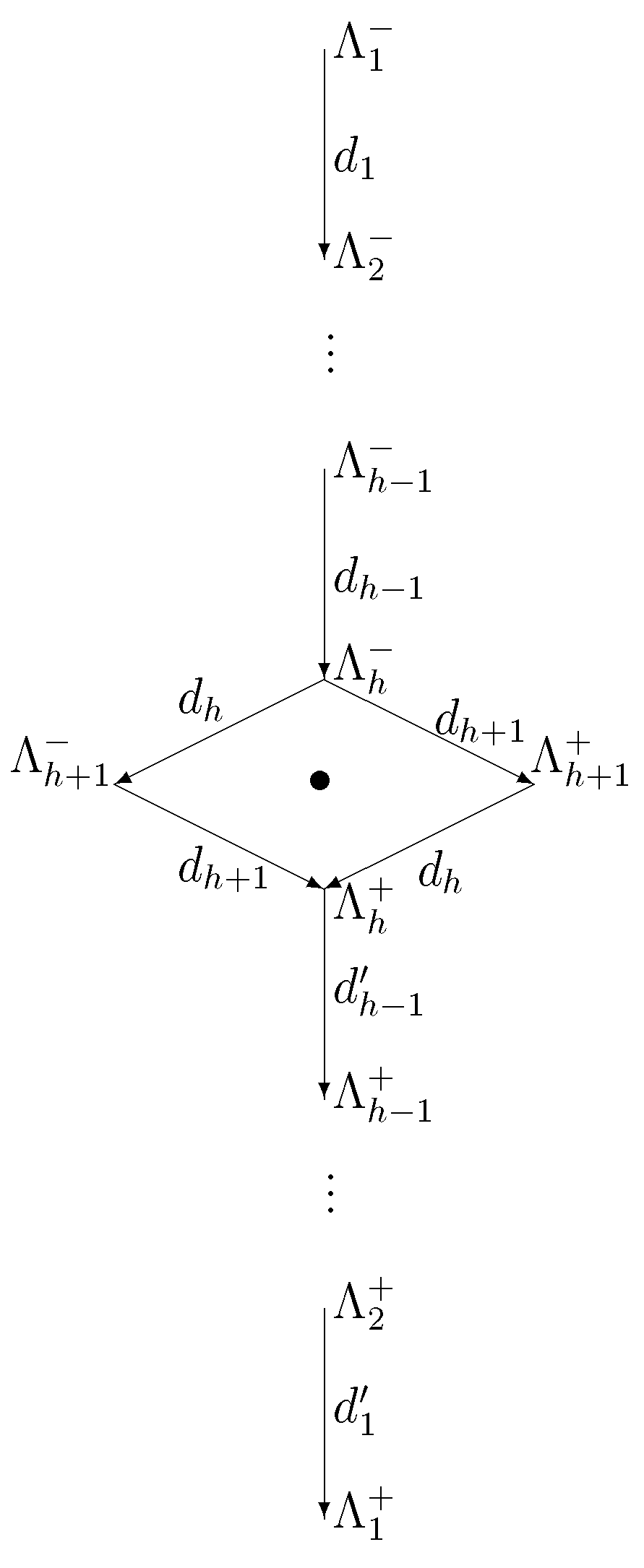
Table 1.
Table of conformal Lie algebras (CLA) with -factor fulfilling (18) and the corresponding parabolically related algebras ; we display also some non-CLA cases.
Table 1.
Table of conformal Lie algebras (CLA) with -factor fulfilling (18) and the corresponding parabolically related algebras ; we display also some non-CLA cases.
| n | ||||
| , | ||||
| , | , | |||
| 27 | ||||
| below not CLA | ||||
| 13 | ||||
| 21 | ||||
| 20 | ||||
| 15 | ||||
| 0 min. | ||||
| max. | ||||
| 6 min. | ||||
| 5 max. |
Disclaimer/Publisher’s Note: The statements, opinions and data contained in all publications are solely those of the individual author(s) and contributor(s) and not of MDPI and/or the editor(s). MDPI and/or the editor(s) disclaim responsibility for any injury to people or property resulting from any ideas, methods, instructions or products referred to in the content. |
© 2024 by the author. Licensee MDPI, Basel, Switzerland. This article is an open access article distributed under the terms and conditions of the Creative Commons Attribution (CC BY) license (https://creativecommons.org/licenses/by/4.0/).
Share and Cite
MDPI and ACS Style
Dobrev, V.K. Canonical Construction of Invariant Differential Operators: A Review. Symmetry 2024, 16, 151. https://doi.org/10.3390/sym16020151
AMA Style
Dobrev VK. Canonical Construction of Invariant Differential Operators: A Review. Symmetry. 2024; 16(2):151. https://doi.org/10.3390/sym16020151
Chicago/Turabian StyleDobrev, Vladimir K. 2024. "Canonical Construction of Invariant Differential Operators: A Review" Symmetry 16, no. 2: 151. https://doi.org/10.3390/sym16020151
Note that from the first issue of 2016, this journal uses article numbers instead of page numbers. See further details here.