Quantum Hall and Shubnikov-de Haas Effects in Graphene within Non-Markovian Langevin Approach

Abstract

The theory of open quantum systems is applied to study galvano-, thermo-magnetic, and magnetization phenomena in axial symmetric two-dimensional systems. Charge carriers are considered as quantum particles interacting with the environment through a one-body (mean-field) mechanism. The dynamics of charge carriers is affected by the average collision time that takes effectively into account two-body effects. The functional dependencies of the average collision time on the external uniform magnetic field, concentration and temperature are phenomenologically treated. Analytical expressions are obtained for the tensors of electric and thermal conductivity and/or resistivity. The developed theory is applied to describe the Shubnikov-de Haas oscillations and quantum Hall effect in graphene and GaAs/Al${}_x$Ga${}_{1-x}$As heterostructure. The dependencies of magnetization and thermal conductivity on the magnetic field are also predicted.

1. Introduction

Emerging new two-dimensional (2D) materials such as heterostructures, graphene, and black phosphorus are considered promising candidates for next-generation electronic, optoelectronic devices, electrode materials, as well as for electrocatalysts in energy storage and electrocatalytic applications [1,2,3,4,5]. One of the fascinating topics in fundamental physics is experimental and theoretical investigations of the properties of 2D electron gas (2DEG) or 2D materials in uniform magnetic fields and at low temperatures. Since the charge carrier mobility in the 2D systems is significantly high, the quantum Hall effects (QHE) and the Shubnikov–de Haas oscillations (SdHO) were observed [6,7,8,9,10,11,12,13]. For example, the QHE appears in the bulk quasi-2D materials like the black-phosphorus [14,15] and the inorganic conductor molybdenum oxide [16] at temperatures of about 0.07–4 K. The oscillator behavior of the diagonal magneto-resistance and the quantization of the off-diagonal resistance $R_{xy}$ at low temperature are interesting phenomena that have not yet been fully understood. External electric and magnetic fields and temperature can change the charge density, mobility, and collision time of charge carriers, as a result of which the transport properties of the latter may change [6]. At low temperatures and a sufficiently strong magnetic field, the SdHO amplitude is large and the QHE plateau is significantly wider [7,8]. For InSb single crystals with different concentrations and n-type mobility in the temperature range from $T_0=4.2$ to 16 K [8], the SdHO amplitude decreases with increasing temperature. It is also clear from the experiment that the period of oscillation remains unchanged at all temperatures. In ref. [13], the experiments with the In${}_{0.53}$Ga${}_{0.47}$As/InP heterostructure were carried out at various low temperatures and found that the Hall plateau disappeared with increasing temperature. The half-width of the oscillations of the diagonal resistance increases, which was also observed in graphene [17,18,19,20,21,22,23,24,25,26], which is a 2D material.

In ref. [17], the integer QHE was discovered in graphene at temperature $T_0=30$ mK. The experimental results obtained show that the mobility of charge carriers in graphene is very high. This, in turn, makes it possible to observe the QHE even at high temperatures. In ref. [20], they even managed to observe QHE under the influence of a very strong magnetic field at room temperature, where the Hall conductivity ${\sigma }_{xy}=2e^2/h$ and the longitudinal conductivity ${\sigma }_{xx}=0$. In ref. [17], the temperature dependence and gate-voltage (charge carriers concentration) dependence of the SdHO in graphene were measured. As obtained, the amplitude of SdHO significantly changes at the magnetic field $B\approx 5$ T. For the SdHO, it would be interesting to investigate theoretically the off-diagonal resistances $R_{xy}$ that correspond to the experimentally obtained diagonal resistances $R_{xx}$ at various magnetic fields and temperatures.

Experimental data show that graphene has a high thermal conductivity ($\kappa \simeq$ 3000–5000 Wm${}^{-1}$K${}^{-1}$ at room temperature) [24]. It depends on the type of substrate, defects, and concentration of impurity atoms [27,28,29,30]. Most experiments on thermal conductivity have usually been carried out at room temperature and higher. Therefore, we are interested in studying the dependence of thermal conductivity on the magnetic field at low temperatures using experimental data on electric conductivity.

In refs. [31,32,33,34], 2D systems in extremely strong magnetic fields were theoretically studied by treating the electron as a free particle and using a scattering potential with short- and long-range scatterers. This model does not work if the 2D system has too much surface roughness. In ref. [35], the Hall conductivity of 2D graphite was theoretically calculated using the Born approximation and analytical expressions for the Hall conductivities were obtained in the cases of short- and long-range scatterers and limits of strong and weak magnetic fields. To date, many experimental and theoretical studies have been carried out, but the theory of QHE is not fully developed.

The purpose of this work is to describe QHE and SdHO in graphene within the non-Markovian quantum Langevin formalism. The main idea of our model is as follows. The charge carriers are considered as quantum particles coupled to the environment (heat bath) through particle-phonon interactions. For example, the substrate of graphene can serve as a heat bath for it. The dynamics of the charge carriers are restricted by the average collision time. The functional forms of the average collision time and relaxation time on temperature, concentration, and magnetic field are extracted from experimental data. Because of this, in reality, the coupling used between the charge carrier and environment is actually more general than a simple particle-phonon coupling. In our model, the one-body, two-body, and non-Markovian effects are taken into consideration. Note, that the quantum Langevin approach was widely used to describe various macroscopic phenomena [36,37,38,39,40,41,42,43,44,45,46].

The work is organized as follows. In Section 2, the main assumptions of the model are discussed. The non-Markovian Langevin equations for the charge carriers embedded in the heat bath and uniform magnetic and electric fields are fully quantum-mechanically derived. Using the solutions of these equations, we obtain time-dependent expressions of the diagonal and non-diagonal electric conductivities in 2D systems. The resulting expressions were analyzed for weak and strong magnetic fields, as well as in the non-Markovian and Markovian limits. In Section 3, we present the description of experimental data on the QHE and SdHO in graphene and GaAs/Al${}_x$Ga${}_{1-x}$As heterostructure. The magnetization and thermal conductivity in graphene are predicted. In Section 4, the main conclusions are given.

2. Non-Markovian Langevin Equations in External Uniform Magnetic and Electric Fields

In order to derive the electric conductivity or resistance tensor for the 2D collective subsystem (charge carrier), a suitable microscopic Hamiltonian,

$$\begin{array}{ccc}\hfill H& =& H_c(B,E_x)+H_b+H_{cb},\hfill \\ \hfill H_c& =& \frac{1}{2m_x}{(p_x-e{A}_x(x,y))}^2+\frac{1}{2m_y}{(p_y-e{A}_y(x,y))}^2+e{E}_{x}x,\hfill \\ \hfill H_b& =& \sum _{\nu }^{}\hslash {\omega }_{\nu }{b}_{\nu }^{+}{b}_{\nu },\hfill \\ \hfill H_{cb}& =& \sum _{\nu }^{}({\alpha }_{\nu }x+g_{\nu }y)(b_{\nu }^{+}+b_{\nu })+\sum _{\nu }^{}\frac{1}{\hslash {\omega }_{\nu }}{({\alpha }_{\nu }x+g_{\nu }y)}^2,\hfill \end{array}$$

(1)

was formulated in ref. [46]. The term $H_c$ is the Hamiltonian of the collective subsystem embedded in the external uniform magnetic and electric fields. Here $\mathbf{q}=(x,y,0)$ is the collective coordinate of a charged particle and $\mathbf{p}=(p_x,p_y,0)$ is its canonically conjugated momentum, $m_x$ and $m_y$ are the components of the effective mass tensor, $\mathbf{A}=(-\frac{1}{2}yB,\frac{1}{2}xB,0)$ is the vector potential of the perpendicular axisymmetric magnetic field (along the z-axis) with the strength $B=\left|\mathbf{B}\right|$, and the constant electric field $\mathbf{E}=(E_x,0,0)$ acting in the x-axis direction (positive charge e). The terms $H_b$ and $H_{cb}$ are the Hamiltonians of the heat bath subsystem, and the collective-bath interaction with the coupling parameters ${\alpha }_{\nu }$ and $g_{\nu }$, respectively. The heat bath is an assembly of harmonic oscillators with frequencies ${\omega }_{\nu }$. The coupling to the heat bath is linear in the phonon creation $b_{\nu }^{+}$ and annihilation $b_{\nu }$ operators and corresponds to the energy being transferred to and from the thermal reservoir by absorption or emission of bath quanta. We introduce the counter-term (second term) in $H_{cb}$ in order to compensate for the coupling-induced potential [38,42].

Introducing new definitions for momenta

$$\begin{array}{c}\hfill {\pi }_x=p_x+\frac{1}{2}{m}_x{\omega }_{cx}y,{\pi }_y=p_y-\frac{1}{2}{m}_y{\omega }_{cy}x,\end{array}$$

(2)

where ${\omega }_{cx}=eB/m_x$ and ${\omega }_{cy}=eB/m_y$ (${\omega }_c=\sqrt{{\omega }_{cx}{\omega }_{cy}}=\frac{eB}{\sqrt{m_x{m}_y}}$ is the cyclotron frequency), we rewrite the Hamiltonian $H_c$ as

$$\begin{array}{ccc}\hfill H_c& =& \frac{{\pi }_x^2}{2m_x}+\frac{{\pi }_y^2}{2m_y}+e{E}_{x}x.\hfill \end{array}$$

(3)

Commuting the collective operators x, y, ${\pi }_x$, ${\pi }_y$, and the bath phonon operators $b_{\nu }$, $b_{\nu }^{+}$ with H, we obtain the system of the Heisenberg equations

$$\begin{array}{ccc}\hfill \dot{x}\left(t\right)& =& \frac{i}{\hslash }[H,x]=\frac{{\pi }_x\left(t\right)}{m_x},\hfill \\ \hfill \dot{y}\left(t\right)& =& \frac{i}{\hslash }[H,y]=\frac{{\pi }_y\left(t\right)}{m_y},\hfill \\ \hfill {\dot{\pi }}_x\left(t\right)& =& \frac{i}{\hslash }[H,{\pi }_x]\hfill \\ & =& {\pi }_y\left(t\right){\omega }_{cy}-e{E}_x-\sum _{\nu }^{}{\alpha }_{\nu }(b_{\nu }^{+}\left(t\right)+b_{\nu }\left(t\right))-2\sum _{\nu }^{}\frac{{\alpha }_{\nu }}{\hslash {\omega }_{\nu }}[{\alpha }_{\nu }x\left(t\right)+g_{\nu }y\left(t\right)],\hfill \\ \hfill {\dot{\pi }}_y\left(t\right)& =& \frac{i}{\hslash }[H,{\pi }_y]\hfill \\ & =& -{\pi }_x\left(t\right){\omega }_{cx}-\sum _{\nu }^{}{g}_{\nu }(b_{\nu }^{+}\left(t\right)+b_{\nu }\left(t\right))-2\sum _{\nu }^{}\frac{g_{\nu }}{\hslash {\omega }_{\nu }}[{\alpha }_{\nu }x\left(t\right)+g_{\nu }y\left(t\right)],\hfill \end{array}$$

(4)

and

$$\begin{array}{ccc}\hfill {\dot{b}}_{\nu }^{+}\left(t\right)& =& \frac{i}{\hslash }[H,b_{\nu }^{+}]=i{\omega }_{\nu }{b}_{\nu }^{+}\left(t\right)+\frac{i}{\hslash }({\alpha }_{\nu }x\left(t\right)+g_{\nu }y\left(t\right)),\hfill \\ \hfill {\dot{b}}_{\nu }\left(t\right)& =& \frac{i}{\hslash }[H,b_{\nu }]=-i{\omega }_{\nu }{b}_{\nu }\left(t\right)-\frac{i}{\hslash }({\alpha }_{\nu }x\left(t\right)+g_{\nu }y\left(t\right)).\hfill \end{array}$$

(5)

Substituting the solution

$$\begin{array}{ccc}\hfill b_{\nu }^{+}\left(t\right)& =& f_{\nu }^{+}\left(t\right)-\frac{{\alpha }_{\nu }x\left(t\right)+g_{\nu }y\left(t\right)}{\hslash {\omega }_{\nu }}\hfill \\ & +& \frac{{\alpha }_{\nu }}{\hslash {\omega }_{\nu }}\underset{0}{\overset{t}{\int }}d\tau \dot{x}\left(\tau \right)e^{i{\omega }_{\nu }(t-\tau )}+\frac{g_{\nu }}{\hslash {\omega }_{\nu }}\underset{0}{\overset{t}{\int }}d\tau \dot{y}\left(\tau \right)e^{i{\omega }_{\nu }(t-\tau )},\hfill \\ \hfill b_{\nu }\left(t\right)& =& f_{\nu }\left(t\right)-\frac{{\alpha }_{\nu }x\left(t\right)+g_{\nu }y\left(t\right)}{\hslash {\omega }_{\nu }}\hfill \\ & +& \frac{{\alpha }_{\nu }}{\hslash {\omega }_{\nu }}\underset{0}{\overset{t}{\int }}d\tau \dot{x}\left(\tau \right)e^{-i{\omega }_{\nu }(t-\tau )}+\frac{g_{\nu }}{\hslash {\omega }_{\nu }}\underset{0}{\overset{t}{\int }}d\tau \dot{y}\left(\tau \right)e^{-i{\omega }_{\nu }(t-\tau )},\hfill \\ \hfill f_{\nu }\left(t\right)& =& [b_{\nu }\left(0\right)+\frac{{\alpha }_{\nu }x\left(0\right)+g_{\nu }y\left(0\right)}{\hslash {\omega }_{\nu }}]e^{-i{\omega }_{\nu }t}\hfill \end{array}$$

(6)

of Equation (5) into (4), we obtain the stochastic dissipative quantum Langevin equations (Heisenberg–Langevin equations)

$$\begin{array}{ccc}\hfill \dot{x}\left(t\right)& =& \frac{{\pi }_x\left(t\right)}{m_x},\hfill \\ \hfill \dot{y}\left(t\right)& =& \frac{{\pi }_y\left(t\right)}{m_y},\hfill \\ \hfill {\dot{\pi }}_x\left(t\right)& =& {\pi }_y\left(t\right){\omega }_{cy}-e{E}_x-\frac{1}{m_x}\underset{0}{\overset{t}{\int }}d\tau K_{\alpha }(t-\tau ){\pi }_x\left(\tau \right)-\frac{1}{m_y}\underset{0}{\overset{t}{\int }}d\tau K_{\alpha g}(t-\tau ){\pi }_y\left(\tau \right)+F_{\alpha }\left(t\right),\hfill \\ \hfill {\dot{\pi }}_y\left(t\right)& =& -{\pi }_x\left(t\right){\omega }_{cx}-\frac{1}{m_y}\underset{0}{\overset{t}{\int }}d\tau K_g(t-\tau ){\pi }_y\left(\tau \right)-\frac{1}{m_x}\underset{0}{\overset{t}{\int }}d\tau K_{g\alpha }(t-\tau ){\pi }_y\left(\tau \right)+F_g\left(t\right)\hfill \end{array}$$

(7)

with the dissipative kernels

$$\begin{array}{ccc}\hfill K_{\alpha }(t-\tau )& =& \sum _{\nu }^{}\frac{2{\alpha }_{\nu }^2}{\hslash {\omega }_{\nu }}\cos \left[{\omega }_{\nu }(t-\tau )\right],K_g(t-\tau )=\sum _{\nu }^{}\frac{2g_{\nu }^2}{\hslash {\omega }_{\nu }}\cos \left[{\omega }_{\nu }(t-\tau )\right],\hfill \\ \hfill K_{\alpha g}(t-\tau )& =& K_{g\alpha }(t-\tau )=\sum _{\nu }^{}\frac{2{\alpha }_{\nu }{g}_{\nu }}{\hslash {\omega }_{\nu }}\cos \left[{\omega }_{\nu }(t-\tau )\right],\hfill \end{array}$$

(8)

and the random forces

$$\begin{array}{ccc}\hfill F_{\alpha }\left(t\right)& =& -\sum _{\nu }{F}_{\alpha }^{\nu }\left(t\right)=-\sum _{\nu }{\alpha }_{\nu }(f_{\nu }^{+}\left(t\right)+f_{\nu }\left(t\right)),\hfill \\ \hfill F_g\left(t\right)& =& -\sum _{\nu }{F}_g^{\nu }\left(t\right)=-\sum _{\nu }{g}_{\nu }(f_{\nu }^{+}\left(t\right)+f_{\nu }\left(t\right))\hfill \end{array}$$

(9)

in the coordinates. The random force operators $F_{\alpha }^{\nu }\left(t\right)$ and $F_g^{\nu }\left(t\right)$ are identified as fluctuations are identified as fluctuations due to the uncertainty of the initial conditions for the thermostat operators. We consider an ensemble of initial states in which the operators of the collective subsystem are fixed at the values $x\left(0\right)$ and $y\left(0\right)$, and the initial bath operators are drawn from an ensemble that is canonical relative to the collective subsystem [39,42]. The initial distribution is then the conditional density matrix ${\rho }_0\left(\{b_{\nu }^{+}\left(0\right),b_{\nu }\left(0\right)\}\right|\mathbf{q}\left(0\right))=exp(-{\sum }_{\nu }^{}\hslash {\omega }_{\nu }[b_{\nu }^{+}+\frac{{\alpha }_{\nu }x+g_{\nu }y}{\hslash {\omega }_{\nu }}][b_{\nu }+\frac{{\alpha }_{\nu }x+g_{\nu }y}{\hslash {\omega }_{\nu }}]/T_0)/Z\left(T_0\right)$, where $Z\left(T_0\right)$ is conditional partition function. In an ensemble of initial states for the bath operators, the fluctuations $F_{\alpha }^{\nu }\left(t\right)$ and $F_g^{\nu }\left(t\right)$ have the Gaussian distributions with zero average value

$$\begin{array}{c}\hfill \ll F_{\alpha }^{\nu }\left(t\right)\gg =\ll F_g^{\nu }\left(t\right)\gg =0,\end{array}$$

(10)

where the symbol $\ll ...\gg$ denotes the average over the bath. The temperature $T_0$ of the heat bath is included in the analysis through the distribution of initial conditions. The Bose-Einstein statistics is employed for the heat bath:

$$\begin{array}{ccc}\hfill \ll f_{\nu }^{+}\left(t\right)f_{{\nu }^{\prime }}^{+}\left(t^{\prime }\right)\gg & =& \ll f_{\nu }\left(t\right)f_{{\nu }^{\prime }}\left(t^{\prime }\right)\gg =0,\hfill \\ \hfill \ll f_{\nu }^{+}\left(t\right)f_{{\nu }^{\prime }}\left(t^{\prime }\right)\gg & =& {\delta }_{\nu ,{\nu }^{\prime }}{n}_{\nu }{e}^{i{\omega }_{\nu }(t-t^{\prime })},\hfill \\ \hfill \ll f_{\nu }\left(t\right)f_{{\nu }^{\prime }}^{+}\left(t^{\prime }\right)\gg & =& {\delta }_{\nu ,{\nu }^{\prime }}(n_{\nu }+1)e^{-i{\omega }_{\nu }(t-t^{\prime })},\hfill \end{array}$$

(11)

where $n_{\nu }={[\exp (\hslash {\omega }_{\nu }/T_0)-1]}^{-1}$ are the occupation numbers for phonons. Employing (11), the quantum fluctuation-dissipation relations are obtained:

$$\sum _{\nu }^{}{\phi }_{\alpha \alpha }^{\nu }(t,t^{\prime })\frac{\tanh \left[\frac{\hslash {\omega }_{\nu }}{2T_0}\right]}{\hslash {\omega }_{\nu }}=K_{\alpha }(t-t^{\prime }),\sum _{\nu }^{}{\phi }_{gg}^{\nu }(t,t^{\prime })\frac{\tanh \left[\frac{\hslash {\omega }_{\nu }}{2T_0}\right]}{\hslash {\omega }_{\nu }}=K_g(t-t^{\prime }),$$

$$\sum _{\nu }^{}{\phi }_{\alpha g}^{\nu }(t,t^{\prime })\frac{\tanh \left[\frac{\hslash {\omega }_{\nu }}{2T_0}\right]}{\hslash {\omega }_{\nu }}=K_{\alpha g}(t-t^{\prime }),$$

where

$${\phi }_{\alpha \alpha }^{\nu }(t,t^{\prime })=2{\alpha }_{\nu }^2[2n_{\nu }+1]\cos \left({\omega }_{\nu }[t-t^{\prime }]\right),{\phi }_{gg}^{\nu }(t,t^{\prime })=2g_{\nu }^2[2n_{\nu }+1]\cos \left({\omega }_{\nu }[t-t^{\prime }]\right),$$

$${\phi }_{\alpha g}^{\nu }(t,t^{\prime })=2{\alpha }_{\nu }{g}_{\nu }[2n_{\nu }+1]\cos \left({\omega }_{\nu }[t-t^{\prime }]\right),$$

are the symmetrized correlation functions ${\phi }_{k{k}^{\prime }}^{\nu }(t,t^{\prime })=\ll F_k^{\nu }\left(t\right)F_{k^{\prime }}^{\nu }\left(t^{\prime }\right)+F_{k^{\prime }}^{\nu }\left(t^{\prime }\right)F_k^{\nu }\left(t\right)\gg$, $k,k^{\prime }=\alpha ,g$. The quantum fluctuation-dissipation relations are reduced to the classical ones in the high-temperature limit (or $\hslash \to 0$): ${\sum }_{\nu }^{}{\phi }_{\alpha \alpha }^{\nu }(t,t^{\prime })=2T_0{K}_{\alpha }(t-t^{\prime })$, ${\sum }_{\nu }^{}{\phi }_{gg}^{\nu }(t,t^{\prime })=2T_0{K}_g(t-t^{\prime })$, and ${\sum }_{\nu }^{}{\phi }_{\alpha g}^{\nu }(t,t^{\prime })=2T_0{K}_{\alpha g}(t-t^{\prime })$.

The presence of the integral parts in Equation (7) indicates non-Markovian dynamics of the system. The dissipative kernels have the form of memory functions since they make the equations of motion at time t dependent on the values of $\dot{x}$ and $\dot{y}$ for previous times. The Laplace transform $\widehat{L}$ of Equation (7) leads to the system of linear equations:

$$\begin{array}{ccc}\hfill x\left(s\right)s& =& x\left(0\right)+\frac{{\pi }_x\left(s\right)}{m_x},\hfill \\ \hfill y\left(s\right)s& =& y\left(0\right)+\frac{{\pi }_y\left(s\right)}{m_y},\hfill \\ \hfill {\pi }_x\left(s\right)s& =& {\pi }_x\left(0\right)+{\omega }_{cy}{\pi }_y\left(s\right)-\frac{e{E}_x}{s}-K_{\alpha }\left(s\right)\frac{{\pi }_x\left(s\right)}{m_x}-K_{\alpha g}\left(s\right)\frac{{\pi }_y\left(s\right)}{m_y}+F_{\alpha }\left(s\right),\hfill \\ \hfill {\pi }_y\left(s\right)s& =& {\pi }_y\left(0\right)-{\omega }_{cx}{\pi }_x\left(s\right)-K_g\left(s\right)\frac{{\pi }_y\left(s\right)}{m_y}-K_{g\alpha }\left(s\right)\frac{{\pi }_x\left(s\right)}{m_x}+F_g\left(s\right).\hfill \end{array}$$

(12)

Here, $K_{\alpha }\left(s\right)$, $K_g\left(s\right)$, $K_{\alpha g}\left(s\right)$, $K_{g\alpha }\left(s\right)$ and $F_{\alpha }\left(s\right)$, $F_g\left(s\right)$ are the Laplace transforms of the dissipative kernels and random forces, respectively. The system of Equation (12) is easy to solve and performs the inverse Laplace transform ${\widehat{L}}^{-1}$ using the residue theorem and the roots of the determinant

$$\begin{array}{ccc}\hfill D& =& s^2+{\omega }_{cx}{\omega }_{cy}+\frac{s{K}_{\alpha }\left(s\right)}{m_x}+\frac{s{K}_g\left(s\right)}{m_y}+\frac{{\omega }_{cy}{K}_{g\alpha }\left(s\right)}{m_x}\hfill \\ & -& \frac{{\omega }_{cx}{K}_{\alpha g}\left(s\right)}{m_y}+\frac{K_{\alpha }\left(s\right)K_g\left(s\right)}{m_x{m}_y}-\frac{K_{\alpha g}\left(s\right)K_{g\alpha }\left(s\right)}{m_x{m}_y}=0.\hfill \end{array}$$

(13)

Finally, the explicit solutions for the originals are

$$\begin{array}{ccc}\hfill x\left(t\right)& =& x\left(0\right)+A_1\left(t\right){\pi }_x\left(0\right)+A_2\left(t\right){\pi }_y\left(0\right)-A_3\left(t\right)e{E}_x+I_x\left(t\right)+I_x^{\prime }\left(t\right),\hfill \\ \hfill y\left(t\right)& =& y\left(0\right)+B_1\left(t\right){\pi }_y\left(0\right)-B_2\left(t\right){\pi }_x\left(0\right)+B_3\left(t\right)e{E}_x-I_y\left(t\right)+I_y^{\prime }\left(t\right),\hfill \\ \hfill {\pi }_x\left(t\right)& =& C_1\left(t\right){\pi }_x\left(0\right)+C_2\left(t\right){\pi }_y\left(0\right)-C_3\left(t\right)e{E}_x+I_{{\pi }_x}\left(t\right)+I_{{\pi }_x}^{\prime }\left(t\right),\hfill \\ \hfill {\pi }_y\left(t\right)& =& D_1\left(t\right){\pi }_y\left(0\right)-D_2\left(t\right){\pi }_x\left(0\right)+D_3\left(t\right)e{E}_x-I_{{\pi }_y}\left(t\right)+I_{{\pi }_y}^{\prime }\left(t\right).\hfill \end{array}$$

(14)

In Equation (14),

$$I_x\left(t\right)={\int }_0^t{A}_1\left(\tau \right)F_{\alpha }(t-\tau )d\tau ,I_x^{\prime }\left(t\right)={\int }_0^t{A}_2\left(\tau \right)F_g(t-\tau )d\tau ,I_y\left(t\right)={\int }_0^t{B}_2\left(\tau \right)F_{\alpha }(t-\tau )d\tau ,$$

$$I_y^{\prime }\left(t\right)={\int }_0^t{B}_1\left(\tau \right)F_g(t-\tau )d\tau ,I_{{\pi }_x}\left(t\right)={\int }_0^t{C}_1\left(\tau \right)F_{\alpha }(t-\tau )d\tau ,I_{{\pi }_x}^{\prime }\left(t\right)={\int }_0^t{C}_2\left(\tau \right)F_g(t-\tau )d\tau ,$$

$$I_{{\pi }_y}\left(t\right)={\int }_0^t{D}_2\left(\tau \right)F_{\alpha }(t-\tau )d\tau ,I_{{\pi }_y}^{\prime }\left(t\right)={\int }_0^t{D}_1\left(\tau \right)F_g(t-\tau )d\tau ,$$

and the time-dependent coefficients

$$\begin{array}{ccc}\hfill A_1\left(t\right)& =& {\widehat{L}}^{-1}\left[\frac{m_{y}s+K_g\left(s\right)}{m_x{m}_{y}D\left(s\right)s}\right]=B_1{|}_{x,\alpha \leftrightarrow y,g},A_2\left(t\right)={\widehat{L}}^{-1}\left[\frac{m_y{\omega }_{cy}-K_{\alpha g}\left(s\right)}{m_x{m}_{y}D\left(s\right)s}\right],\hfill \\ \hfill A_3\left(t\right)& =& {\widehat{L}}^{-1}\left[\frac{m_{y}s+K_g\left(s\right)}{m_x{m}_{y}D\left(s\right)s^2}\right],B_2\left(t\right)={\widehat{L}}^{-1}\left[\frac{m_x{\omega }_{cx}+K_{g\alpha }\left(s\right)}{m_x{m}_{y}D\left(s\right)s}\right],\hfill \\ \hfill B_3\left(t\right)& =& {\widehat{L}}^{-1}\left[\frac{m_x{\omega }_{cx}+K_{g\alpha }\left(s\right)}{m_x{m}_{y}D\left(s\right)s^2}\right],C_1\left(t\right)={\widehat{L}}^{-1}\left[\frac{m_{y}s+K_g\left(s\right)}{m_{y}D\left(s\right)}\right]=D_1{|}_{x,\alpha \leftrightarrow y,g},\hfill \\ \hfill C_2\left(t\right)& =& {\widehat{L}}^{-1}\left[\frac{m_y{\omega }_{cy}-K_{\alpha g}\left(s\right)}{m_{y}D\left(s\right)}\right],C_3\left(t\right)={\widehat{L}}^{-1}\left[\frac{m_{y}s+K_g\left(s\right)}{m_{y}D\left(s\right)s}\right],\hfill \\ \hfill D_2\left(t\right)& =& {\widehat{L}}^{-1}\left[\frac{m_x{\omega }_{cx}+K_{g\alpha }\left(s\right)}{m_{x}D\left(s\right)}\right],D_3\left(t\right)={\widehat{L}}^{-1}\left[\frac{m_x{\omega }_{cx}+K_{g\alpha }\left(s\right)}{m_{x}D\left(s\right)s}\right].\hfill \end{array}$$

(15)

In general, the diagonal dissipative kernels are much larger than off-diagonal ones. For simplicity, we assume that there is no correlation between the operators $F_{\alpha }^{\nu }$ and $F_g^{\nu }$, so that $K_{\alpha g}=K_{g\alpha }=0$. We introduce the spectral density $D_{\omega }$ of the heat bath excitations to replace the sum over $\nu$ by the integral over frequency $\omega$: ${\sum }_{\nu }^{}...\to \underset{0}{\overset{\infty }{\int }}d\omega D_{\omega }...$, ${\alpha }_{\nu }\to {\alpha }_{\omega }$, $g_{\nu }\to g_{\omega }$, ${\omega }_{\nu }\to \omega$, and $n_{\nu }\to n_{\omega }$. The well-known spectral functions [36,39,42]

$$\begin{array}{c}\hfill D_{\omega }\frac{{\alpha }_{\omega }^2}{\omega }=\frac{{\lambda }_x^2}{\pi }\frac{{\gamma }^2}{{\gamma }^2+{\omega }^2},D_{\omega }\frac{g_{\omega }^2}{\omega }=\frac{{\lambda }_y^2}{\pi }\frac{{\gamma }^2}{{\gamma }^2+{\omega }^2}\end{array}$$

(16)

are used. Here, the memory time ${\gamma }^{-1}$ of dissipation is inverse to the phonon bandwidth of the heat bath excitations and the coefficients

$$\begin{array}{c}\hfill {\lambda }_x=\frac{1}{m_x}{\int }_0^{\infty }d\tau K_{\alpha }(t-\tau ),{\lambda }_y=\frac{1}{m_y}{\int }_0^{\infty }d\tau K_g(t-\tau )\end{array}$$

are the friction coefficients in the Markovian limit. This Ohmic dissipation with the Lorenzian cutoff (Drude dissipation) results in the dissipative kernels

$$\begin{array}{c}\hfill K_{\alpha }\left(t\right)=m_x{\lambda }_x\gamma e^{-\gamma \left|t\right|},K_g\left(t\right)=m_y{\lambda }_y\gamma e^{-\gamma \left|t\right|}.\end{array}$$

(17)

So, the solutions for the collective coordinates (14) include the following time-dependent coefficients

$$\begin{array}{ccc}\hfill A_1\left(t\right)& =& {\dot{A}}_3\left(t\right),A_2\left(t\right)={\dot{B}}_3{\left(t\right)|}_{x\leftrightarrow y},\hfill \\ \hfill A_3\left(t\right)& =& \frac{1}{m_x}\left(\frac{{\lambda }_{y}t}{{\omega }_c^2+{\lambda }_x{\lambda }_y}+\frac{{\omega }_c^2\left(\gamma -{\lambda }_y\right)-{\lambda }_y^2\left(\gamma -{\lambda }_x\right)}{\gamma {\left({\omega }_c^2+{\lambda }_x{\lambda }_y\right)}^2}\right.\hfill \\ & +& \left.\sum _{i=1}^4\frac{{\beta }_i(s_i+\gamma )\left(\gamma {\lambda }_y+s_i(s_i+\gamma )\right)e^{s_{i}t}}{s_i^2}\right),\hfill \\ \hfill B_1\left(t\right)& =& {\dot{A}}_3{\left(t\right)|}_{x\leftrightarrow y},B_2\left(t\right)={\dot{B}}_3\left(t\right),\hfill \\ \hfill B_3\left(t\right)& =& \frac{{\omega }_{cx}}{m_y}\left(\frac{t}{{\omega }_c^2+{\lambda }_x{\lambda }_y}+\frac{2{\lambda }_x{\lambda }_y-\gamma ({\lambda }_x+{\lambda }_y)}{\gamma {\left({\omega }_c^2+{\lambda }_x{\lambda }_y\right)}^2}+\sum _{i=1}^4\frac{{\beta }_i{(s_i+\gamma )}^2{e}^{s_{i}t}}{s_i^2}\right),\hfill \\ \hfill C_1\left(t\right)& =& m_x{\ddot{A}}_3\left(t\right),C_2\left(t\right)=m_x{\ddot{B}}_3{\left(t\right)|}_{x\leftrightarrow y},C_3\left(t\right)=m_x{\dot{A}}_3\left(t\right),\hfill \\ \hfill D_1\left(t\right)& =& C_1\left(t\right){{|}_{x\leftrightarrow y},D_2\left(t\right)=C_2\left(t\right)|}_{x\leftrightarrow y},D_3\left(t\right)=m_y{\dot{B}}_3\left(t\right),\hfill \end{array}$$

(18)

where ${\beta }_i={\left[{\prod }_{j\ne i}(s_i-s_j)\right]}^{-1}$ ($i,j=1-4$) and $s_i$ are the roots of the equation

$$\begin{array}{ccc}\hfill D\left(s\right)& =& (s+\gamma )\left[(s^2+{\omega }_c^2)(s+\gamma )+s\gamma {\lambda }_x\right]+\gamma {\lambda }_y\left[s(s+\gamma )+\gamma {\lambda }_x\right]=0.\hfill \end{array}$$

(19)

These roots arise when the residue theorem is applied to perform the integration in the inverse Laplace transform ${\widehat{L}}^{-1}$.

The system of equations for the first moments

$$\begin{array}{ccc}\hfill \langle \dot{x}\left(t\right)\rangle & =& \frac{\langle {\pi }_x\left(t\right)\rangle }{m_x},\langle \dot{y}\left(t\right)\rangle =\frac{\langle {\pi }_y\left(t\right)\rangle }{m_y}\hfill \\ \hfill \langle {\dot{\pi }}_x\left(t\right)\rangle & =& {\tilde{\omega }}_{cy}\left(t\right)\langle {\pi }_y\left(t\right)\rangle -{\lambda }_{{\pi }_x}\left(t\right)\langle {\pi }_x\left(t\right)\rangle -e{\tilde{E}}_{xx}\left(t\right),\hfill \\ \hfill \langle {\dot{\pi }}_y\left(t\right)\rangle & =& -{\tilde{\omega }}_{cx}\left(t\right)\langle {\pi }_x\left(t\right)\rangle -{\lambda }_{{\pi }_y}\left(t\right)\langle {\pi }_y\left(t\right)\rangle -e{\tilde{E}}_{xy}\left(t\right)\hfill \end{array}$$

(20)

is derived by averaging Equation (14) over the entire system and differentiating them with respect to t. In Equation (20),

$$\begin{array}{ccc}\hfill {\lambda }_{{\pi }_x}\left(t\right)& =& -\frac{D_1\left(t\right){\dot{C}}_1\left(t\right)+D_2\left(t\right){\dot{C}}_2\left(t\right)}{C_1\left(t\right)D_1\left(t\right)+C_2\left(t\right)D_2\left(t\right)},\hfill \\ \hfill {\lambda }_{{\pi }_y}\left(t\right)& =& -\frac{C_1\left(t\right){\dot{D}}_1\left(t\right)+C_2\left(t\right){\dot{D}}_2\left(t\right)}{C_1\left(t\right)D_1\left(t\right)+C_2\left(t\right)D_2\left(t\right)},\hfill \end{array}$$

(21)

$$\begin{array}{ccc}\hfill {\tilde{\omega }}_{cx}\left(t\right)& =& \frac{D_1\left(t\right){\dot{D}}_2\left(t\right)-D_2\left(t\right){\dot{D}}_1\left(t\right)}{C_1\left(t\right)D_1\left(t\right)+C_2\left(t\right)D_2\left(t\right)},\hfill \\ \hfill {\tilde{\omega }}_{cy}\left(t\right)& =& \frac{C_1\left(t\right){\dot{C}}_2\left(t\right)-C_2\left(t\right){\dot{C}}_1\left(t\right)}{C_1\left(t\right)D_1\left(t\right)+C_2\left(t\right)D_2\left(t\right)},\hfill \end{array}$$

(22)

and

$$\begin{array}{ccc}\hfill {\tilde{E}}_{xx}\left(t\right)& =& E_x\left[D_3\left(t\right){\tilde{\omega }}_{cy}+C_3\left(t\right){\lambda }_{{\pi }_x}\left(t\right)+{\dot{C}}_3\left(t\right)\right],\hfill \\ \hfill {\tilde{E}}_{xy}\left(t\right)& =& E_x\left[C_3\left(t\right){\tilde{\omega }}_{cx}-D_3\left(t\right){\lambda }_{{\pi }_y}\left(t\right)-{\dot{D}}_3\left(t\right)\right]\hfill \end{array}$$

(23)

are the friction coefficients, renormalized cyclotron frequencies, and the components of the electric field, respectively. As seen, the cross-component (along the y-axis) of the electric field ${\tilde{E}}_{xy}\left(t\right)$ is equal to zero at $t=0$ and only arises during the non-Markovian evolution of charge carriers, and ${\tilde{E}}_{xy}(t\to \infty )\ne 0$ (the classical Hall effect). Note that ${\tilde{E}}_{xy}\left(t\right)=0$ in the Markovian limit ($\gamma \to \infty$) [46].

One can define the current density ($k,l=x,y$) [6]

$$\begin{array}{ccc}\hfill J_k& =& \sum _l^{}{\sigma }_{kl}\left(B\right)E_l\hfill \end{array}$$

(24)

by using the expression $\mathbf{J}=ne\langle \dot{\mathbf{q}}\left(t\right)\rangle$ and Equation (20):

$$\begin{array}{ccc}\hfill J_x& =& \frac{n{e}^2}{m_x}{C}_3\left(t\right)E_x\left(t\right),J_y=-\frac{n{e}^2}{m_y}{D}_3\left(t\right)E_x\left(t\right).\hfill \end{array}$$

(25)

Changing the direction of the electric field $\mathbf{E}=(E_x,0,0)$ to $\mathbf{E}=(0,E_y,0)$, we obtain

$$\begin{array}{ccc}\hfill J_x& =& \frac{n{e}^2}{m_x}{\tilde{D}}_3\left(t\right)E_y\left(t\right),J_y=\frac{n{e}^2}{m_y}{\tilde{C}}_3\left(t\right)E_y\left(t\right),\hfill \end{array}$$

(26)

where

$$\begin{array}{ccc}\hfill {\tilde{C}}_3\left(t\right)& =& m_y{L}^{-1}\left[\frac{K_{xx}\left(s\right)+m_{x}s}{D}\right],{\tilde{D}}_3=m_x{m}_y{\omega }_{cy}{L}^{-1}\left[\frac{1}{D}\right].\hfill \end{array}$$

(27)

From (24)–(26) we obtain the expression for the conductivity tensor

$$\begin{array}{ccc}\hfill \sigma \left(\tau \right)& =& n{e}^2\left(\begin{array}{cc}\frac{C_3\left(\tau \right)}{m_x}& -\frac{D_3\left(\tau \right)}{m_y}\\ \frac{{\tilde{D}}_3\left(\tau \right)}{m_x}& \frac{{\tilde{C}}_3\left(\tau \right)}{m_y}\end{array}\right)\hfill \end{array}$$

(28)

at time $\tau$. The inverse transformation of $\sigma \left(\tau \right)$ results in the resistance tensor

$$\begin{array}{ccc}\hfill R\left(\tau \right)& =& \frac{1}{n{e}^2\left[C_3\left(\tau \right){\tilde{C}}_3\left(\tau \right)+D_3\left(\tau \right){\tilde{D}}_3\left(\tau \right)\right]}\left(\begin{array}{cc}{m}_x{\tilde{C}}_3\left(\tau \right)& m_x{D}_3\left(\tau \right)\\ -m_y{\tilde{D}}_3\left(\tau \right)& m_y{C}_3\left(\tau \right)\end{array}\right).\hfill \end{array}$$

(29)

The non-diagonal elements

$$\begin{array}{ccc}\hfill R_H\left(\tau \right)& =& \frac{m_x{D}_3\left(\tau \right)}{n{e}^2\left[C_3\left(\tau \right){\tilde{C}}_3\left(\tau \right)+D_3\left(\tau \right){\tilde{D}}_3\left(\tau \right)\right]}=\frac{m_y{\tilde{D}}_3\left(\tau \right)}{n{e}^2\left[C_3\left(\tau \right){\tilde{C}}_3\left(\tau \right)+D_3\left(\tau \right){\tilde{D}}_3\left(\tau \right)\right]}\hfill \end{array}$$

(30)

of the $R\left(\tau \right)$ have the meaning of the Hall resistance.

In order to describe the magnetotransport in real 2D systems, we need to use some additional assumptions [46]:

(1)

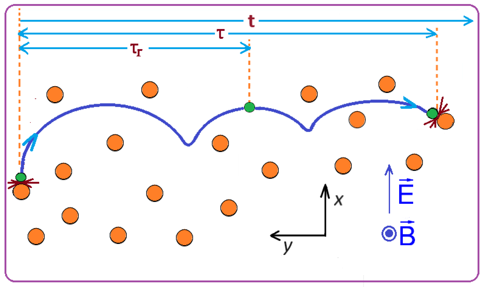
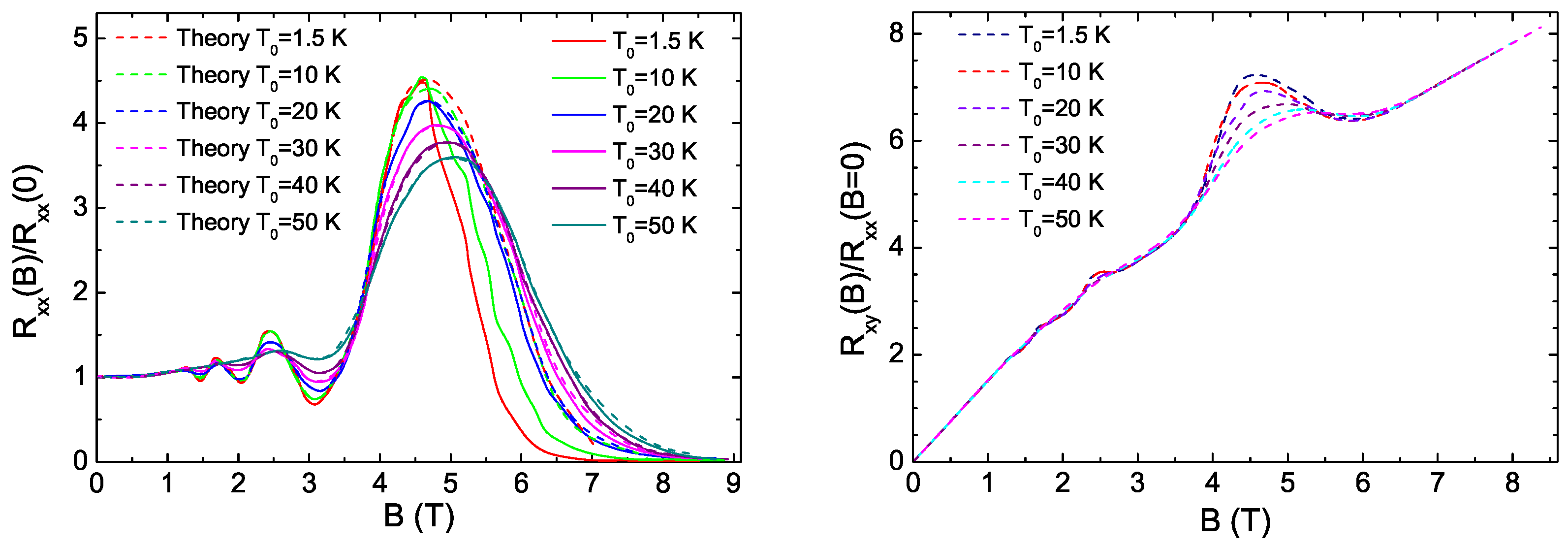
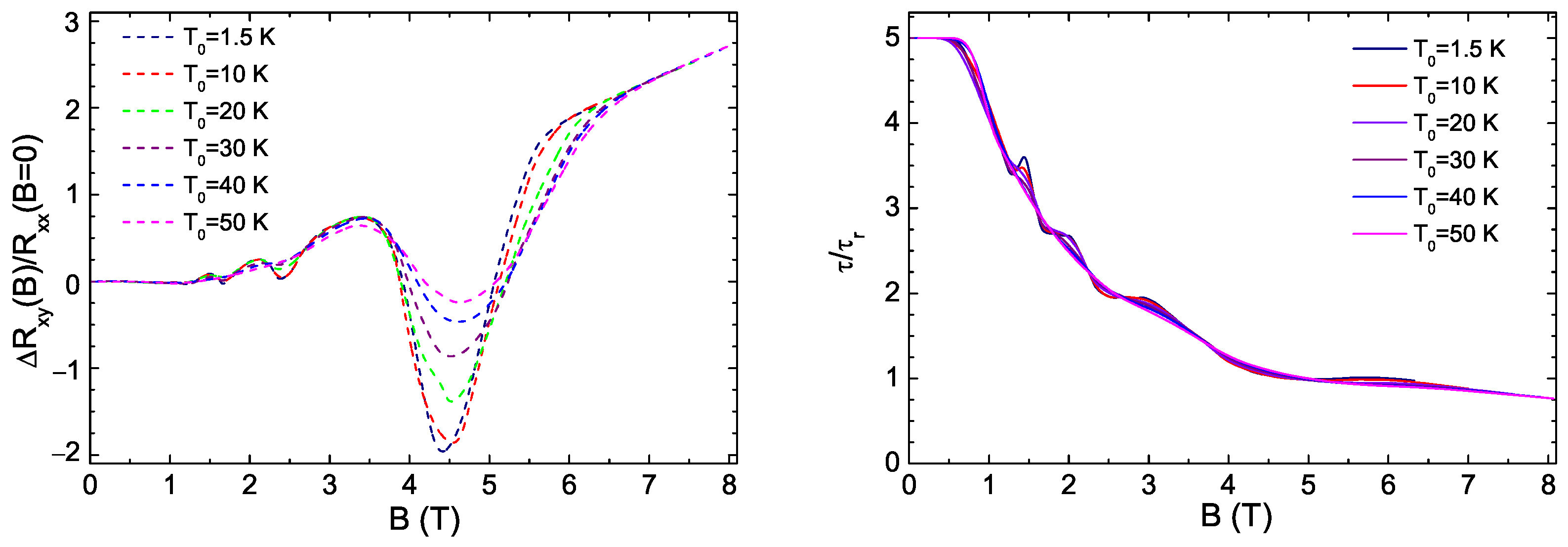
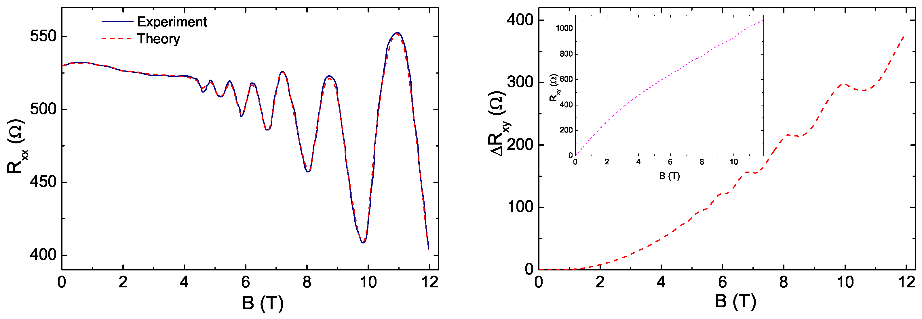
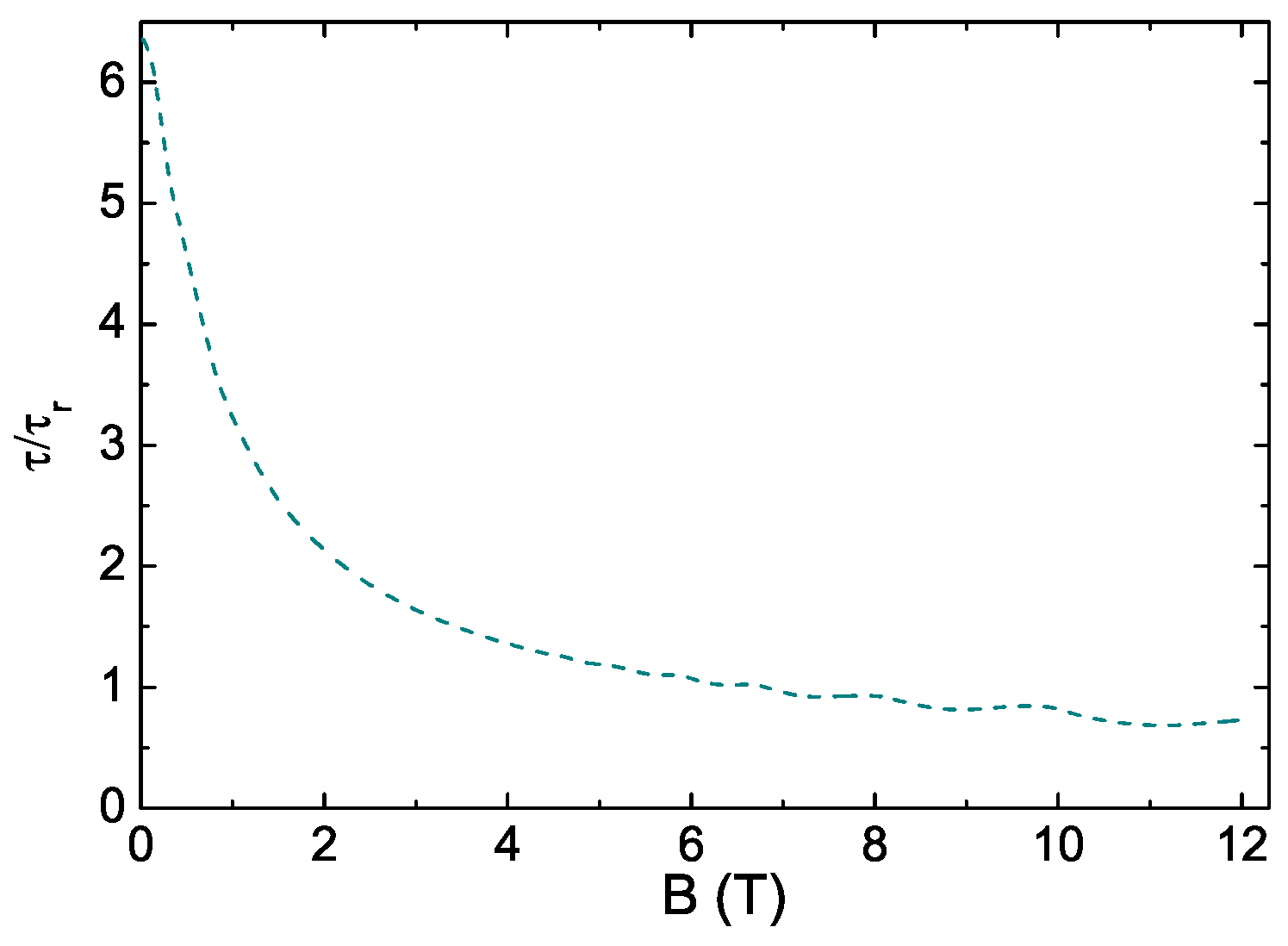
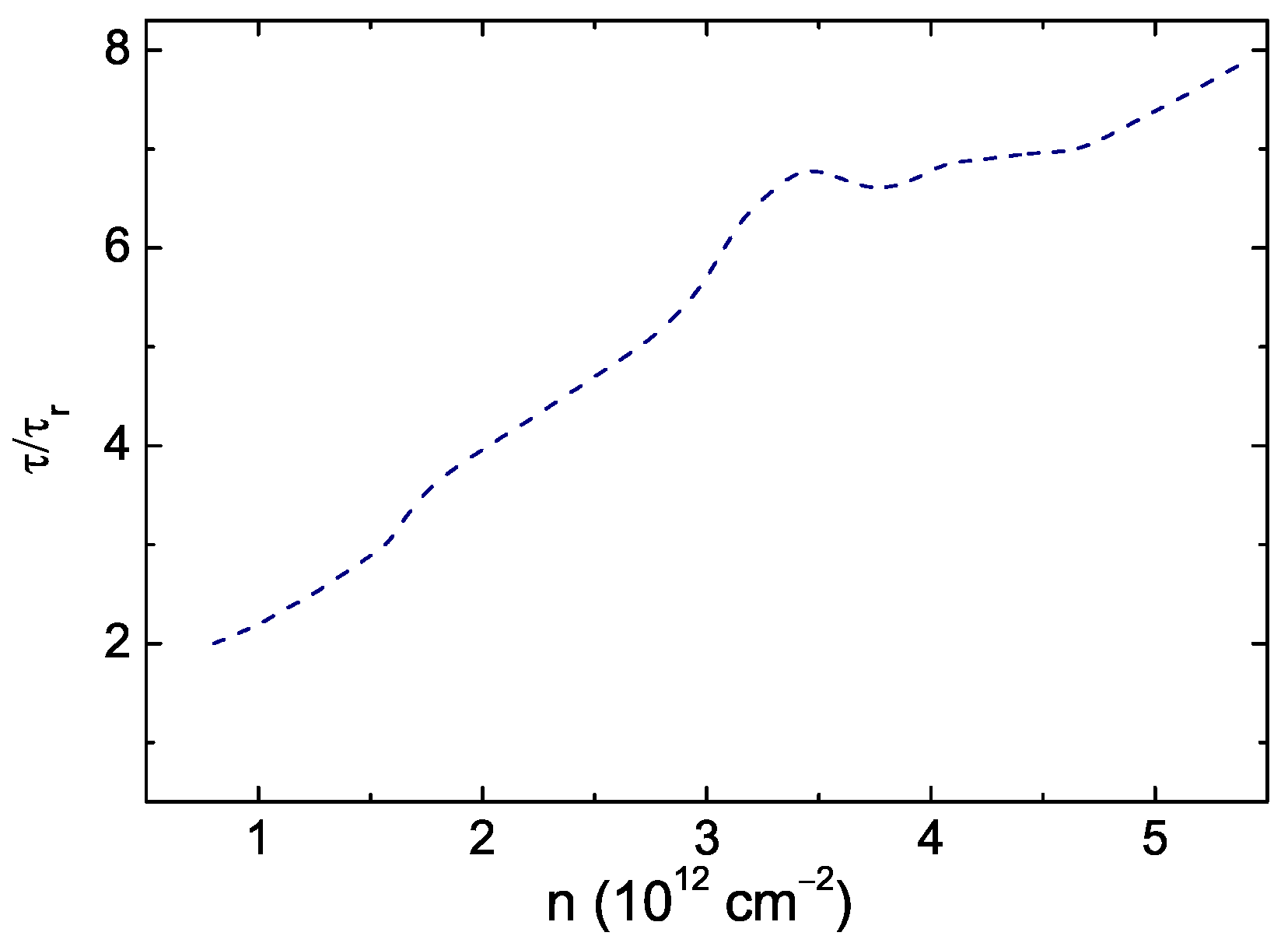
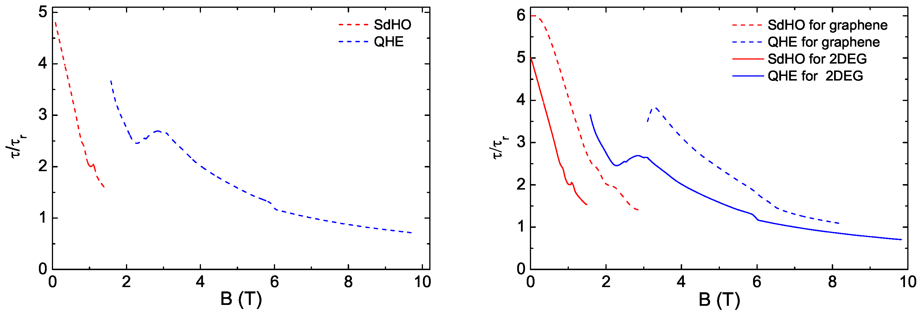
The dynamics of charge carriers are determined by three main characteristic times: the relaxation time ${\tau }_r={\lambda }^{-1}$ (if ${\lambda }_x={\lambda }_y=\lambda$), the average time $\tau$ of a free path (or the average collision time of a charge carrier between two successive collisions with ions/atoms of the lattice), and the memory time ${\gamma }^{-1}$ of the heat bath excitations. The values of ${\tau }_r$ and $\tau$ are associated with one-body (mean-field) and two-body dissipations (effects), respectively (see Figure 1). At $\tau \gg {\tau }_r$ (${\tau }_r\gg \tau$), one-body (two-body) dissipation dominates. If the values of ${\tau }_r$ and $\tau$ are comparable, then the transition process takes place. In general, the values of ${\tau }_r$ and $\tau$ depend on the magnetic field B, temperature $T_0$, and concentration n. Since these relationships are extracted from known experimental data, the coupling used between the charge carrier and environment is actually more general than the particle-phonon interaction.

(2)

Since the mass of the charge carrier is negligibly small compared to the mass of the ion/atom, it can be assumed that with each collision with the ion/atom, the charge carrier completely loses its ordered motion and its velocity or momentum becomes equal to zero. The times $\tau$ of a free path are assumed to be the same for all charge carriers and all collisions. Thus, the time limit $t=\tau$ is introduced in the conductivity tensor (28) or resistance tensor (29).

For the space-symmetric system ($m_x=m_y=m$, ${\lambda }_x={\lambda }_y=\lambda$), we derive analytical expressions that help us clarify our model and the magnetotransport process. In this case, Equation (19) simplifies as

$$\begin{array}{c}\hfill \left(s^2+{\omega }_c^2\right){\left(\gamma +s\right)}^2+2\gamma \lambda s\left(\gamma +s\right)+{\lambda }^2{\gamma }^2=0.\end{array}$$

(31)

The roots of this equation are

$$\begin{array}{ccc}\hfill s_1& =& -\frac{1}{2}\left(\gamma +i{\omega }_c+\sqrt{{\left(\gamma -i{\omega }_c\right)}^2-4\gamma \lambda }\right),s_2=s_1^{*},\hfill \\ \hfill s_3& =& -\frac{1}{2}\left(\gamma +i{\omega }_c-\sqrt{{\left(\gamma -i{\omega }_c\right)}^2-4\gamma \lambda }\right),s_4=s_3^{*}.\hfill \end{array}$$

Expanding these roots up to the first order in $\lambda /\gamma$,

$$\begin{array}{c}\hfill s_1=s_2^{*}=-\gamma \frac{{\omega }_c^2+{\gamma }^2-\gamma \lambda }{{\gamma }^2+{\omega }_c^2}+i\frac{\lambda \gamma {\omega }_c}{{\gamma }^2+{\omega }_c^2},s_3=s_4^{*}=-\frac{\lambda {\gamma }^2}{{\gamma }^2+{\omega }_c^2}-i\frac{{\omega }_c^2+{\gamma }^2+\gamma \lambda }{{\gamma }^2+{\omega }_c^2}{\omega }_c,\end{array}$$

(32)

and taking them at $t=\tau$, we obtain the diagonal and off-diagonal components of conductivity

$$\begin{array}{ccc}\hfill {\sigma }_{xx}\left(\tau \right)& =& \frac{{\sigma }_{xx0}}{1+{\left({\omega }_c{\tau }_r\right)}^2}-\frac{{\sigma }_{xx0}}{\sqrt{1+{\left({\omega }_c{\tau }_r\right)}^2}}\hfill \\ & \times & \exp [-\frac{{\gamma }^2}{{\gamma }^2+{\omega }_c^2}\frac{\tau }{{\tau }_r}]\cos [\frac{\left({\gamma }^2+\gamma /{\tau }_r+{\omega }_c^2\right){\omega }_c\tau }{{\gamma }^2+{\omega }_c^2}+\arctan \left({\omega }_c{\tau }_r\right)],\hfill \\ \hfill {\sigma }_{xy}\left(\tau \right)& =& -\frac{{\sigma }_{xx0}{\omega }_c{\tau }_r}{1+{\left({\omega }_c{\tau }_r\right)}^2}+\frac{{\sigma }_{xx0}}{\sqrt{1+{\left({\omega }_c{\tau }_r\right)}^2}}\hfill \\ & \times & \exp [-\frac{{\gamma }^2}{{\gamma }^2+{\omega }_c^2}\frac{\tau }{{\tau }_r}]\cos [\frac{\left({\gamma }^2+\gamma /{\tau }_r+{\omega }_c^2\right){\omega }_c\tau }{{\gamma }^2+{\omega }_c^2}-\arctan (\frac{1}{{\omega }_c{\tau }_r})].\hfill \end{array}$$

(33)

As seen, Equation (33) contain the non-oscillatory and oscillatory components. If the values of ${\tau }_r$ and $\tau$ are comparable, the non-oscillatory terms of (33) have a major role. In the Markovian limit ($\gamma \to \infty$), Equation (33) are transformed to simpler expressions:

$$\begin{array}{ccc}\hfill {\sigma }_{xx}\left(\tau \right)& =& \frac{{\sigma }_{xx0}}{1+{\left({\omega }_c{\tau }_r\right)}^2}-\frac{{\sigma }_{xx0}}{\sqrt{1+{\left({\omega }_c{\tau }_r\right)}^2}}\exp [-\frac{\tau }{{\tau }_r}]\cos [{\omega }_c\tau +\arctan \left({\omega }_c{\tau }_r\right)],\hfill \\ \hfill {\sigma }_{xy}\left(\tau \right)& =& -\frac{{\sigma }_{xx0}{\omega }_c{\tau }_r}{1+{\left({\omega }_c{\tau }_r\right)}^2}+\frac{{\sigma }_{xx0}}{\sqrt{1+{\left({\omega }_c{\tau }_r\right)}^2}}\exp [-\frac{\tau }{{\tau }_r}]\cos [{\omega }_c\tau -\arctan (\frac{1}{{\omega }_c{\tau }_r})].\hfill \end{array}$$

(34)

At $\tau \gg {\tau }_r$ or $t\to \infty$, the oscillatory terms vanish and we obtain the Drude conductivity tensor

$$\begin{array}{ccc}\hfill \sigma & =& \frac{{\sigma }_{xx0}}{1+{\left({\omega }_c{\tau }_r\right)}^2}\left(\begin{array}{cc}1& -{\omega }_c{\tau }_r\\ {\omega }_c{\tau }_r& 1\end{array}\right)\hfill \end{array}$$

(35)

with the Drude conductivity

$$\begin{array}{ccc}\hfill {\sigma }_{xx0}& =& \frac{n{e}^2{\tau }_r}{m}\hfill \end{array}$$

(36)

at $B=0$. Thus, one can say that our model is the generalized Drude model.

3. Calculated Results

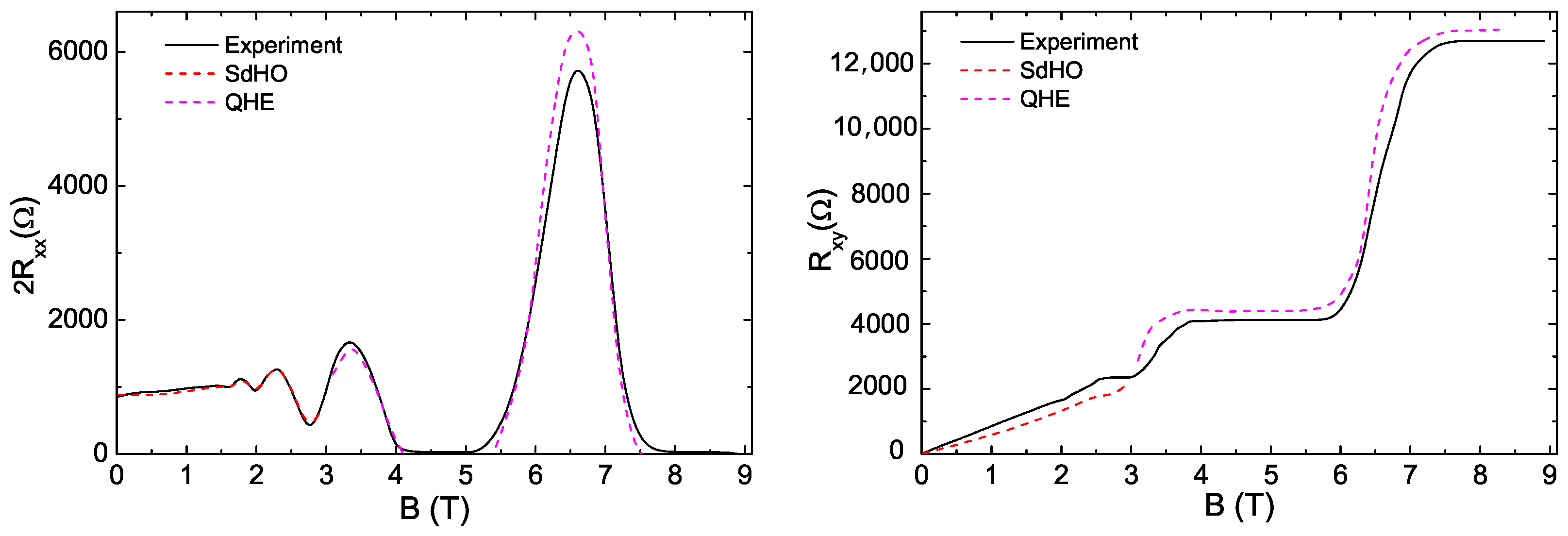
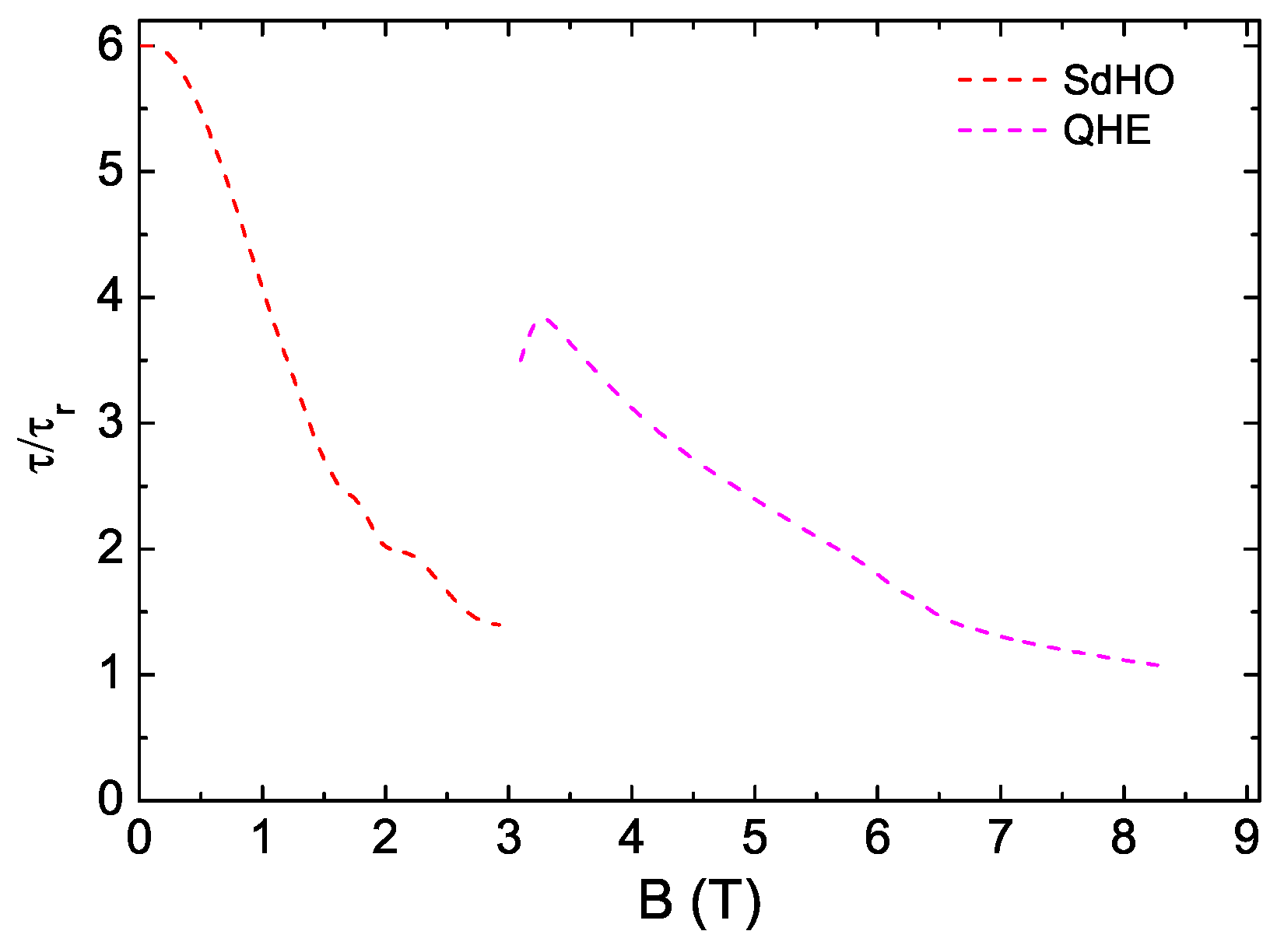
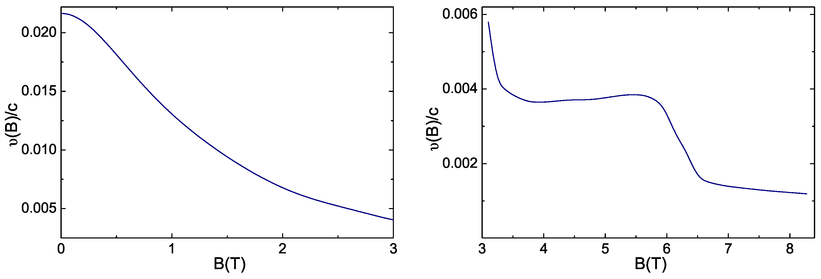
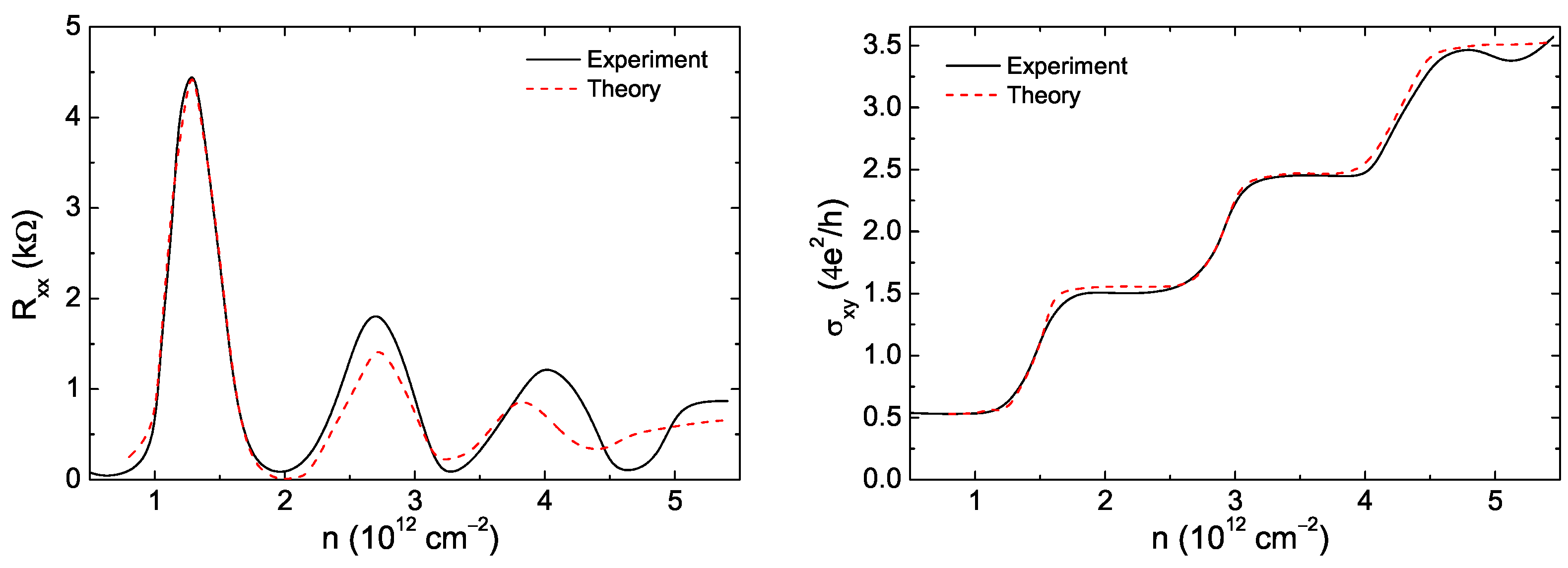
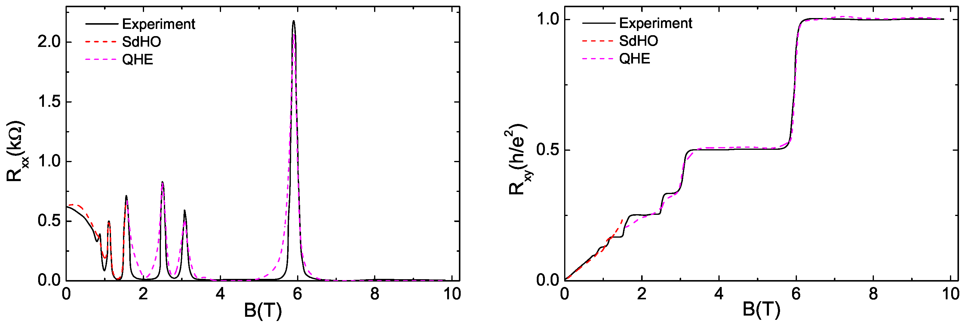
In order to turn to the observable values, all parameters ${\tau }^{-1},{\tau }_r^{-1}$, ${\omega }_c$, and $\gamma$ in the expressions are multiplied by $m/e$:

$$\begin{array}{c}\hfill {\tau }^{-1}\to \frac{m}{e}{\tau }^{-1},{\tau }_r^{-1}\to \frac{m}{e}{\tau }_r^{-1}={\mu }^{-1},\\ \hfill {\omega }_c\to \frac{m}{e}{\omega }_c=B,\gamma \to \frac{m}{e}\gamma =\Gamma .\end{array}$$

(37)

So instead of the friction coefficient $\lambda$, cyclotron frequency ${\omega }_c$, and the inverse response time $\gamma$ of the system, we have the inverse reciprocal mobility ${\mu }^{-1}$ of charge carriers, the strength of the magnetic field B, and a new parameter $\Gamma$ related to the memory time. However, for the graphene and 2D heterostructures considered, the mobility is almost independent of B (here $\mu \left(B\right)={\mu }_0$ and ${\mu }_0=\mu (B=0)$) in a wide range of B. So, their properties are described by neglecting the effect of the magnetic field on the coupling term.

3.1. SdHO and QHE

The dependence of magnetoresistance ($R_{xx}$) and Hall resistance ($R_{xy}$) on the magnetic field is shown in Figure 2 for a wide range of magnetic fields. Experimental results are taken from ref. [17], and theoretical calculations are performed using formula (29) with $\Gamma =13/(\tau /{\tau }_r)$. The experiment is conducted at the temperature $T_0=30$ mK and the gate voltage $V_g=15$ V applied to the graphene sample. The charge carriers consist of electrons and they have very high mobility, which is $\mu$ = 13,000 cm${}^2$V${}^{-1}$s${}^{-1}$ and it weakly depends on the magnetic field and temperature. The SiO${}_2$ is taken as a substrate, and the carrier density is controlled by applying a gate voltage $V_g$ ($n=\alpha V_g$, where $\alpha \approx 7.3\times {10}^{10}$ cm${}^{-2}$V${}^{-1}$[19]). The average collision times $\tau$ are extracted using the experimental data.

In Figure 2, the SdHO is observed in a narrow range of magnetic fields ($B\le 3$ T), and the QHE is observed at strong magnetic fields ($B>3$ T), where the longitudinal resistance has a minimum, and the Hall resistance has a plateau. As seen, our model describes both SdHO and QHE. The calculated results show that the values of $\tau /{\tau }_r$ are different for both processes (see Figure 3). The value of $\tau /{\tau }_r$ for SdHO decreases with the magnetic field and approaches unity at $B=3$ T. At the beginning of the QHE (at $B\approx 3$ T), a phase transition is observed, in which the value of $\tau /{\tau }_r$ increases several times compared to the value of $\tau /{\tau }_r$ at the end of the SdHO process. In the case of QHE, the value of $\tau /{\tau }_r$ decreases slower with increasing magnetic field than in the case of SdHO. As follows from Figure 3, the SdHO and QHE are the results of the transitional processes because the values of ${\tau }_r$ and $\tau$ are comparable. The observed wide plateau in $R_{xy}$ at strong fields can be explained by a decrease in the average collision time of charge carriers.

In the QHE, in the region between two plateaus in $R_{xy}$, the longitudinal resistance $R_{xx}$ has a maximum, while in the center of the plateau, it is a minimum. This phenomenon is explained by antiphase oscillations of $R_{xx}$ and $R_{xy}$, which are clearly visible in the approximate formulas

$$\begin{array}{ccc}\hfill R_{xx}\left(B\right)& =& \frac{R_{xx0}\left(1+\mu B\exp \left[-\frac{{\Gamma }^2}{{\Gamma }^2+B^2}\frac{\tau }{{\tau }_r}\right]\sin \left[\frac{\left({\Gamma }^2+\Gamma /\mu +B^2\right)\mu B}{{\Gamma }^2+B^2}\frac{\tau }{{\tau }_r}\right]\right)}{1+\exp \left[-\frac{2{\Gamma }^2}{{\Gamma }^2+B^2}\frac{\tau }{{\tau }_r}\right]-2\exp \left[-\frac{{\Gamma }^2}{{\Gamma }^2+B^2}\frac{\tau }{{\tau }_r}\right]\cos \left[\frac{\left({\Gamma }^2+\Gamma /\mu +B^2\right)\mu B}{{\Gamma }^2+B^2}\frac{\tau }{{\tau }_r}\right]},\hfill \\ \hfill R_{xy}\left(B\right)& =& \frac{R_{xx0}\mu B\left(1-\exp \left[-\frac{{\Gamma }^2}{{\Gamma }^2+B^2}\frac{\tau }{{\tau }_r}\right]\cos \left[\frac{\left({\Gamma }^2+\Gamma /\mu +B^2\right)\mu B}{{\Gamma }^2+B^2}\frac{\tau }{{\tau }_r}\right]\right)}{1+\exp \left[-\frac{2{\Gamma }^2}{{\Gamma }^2+B^2}\frac{\tau }{{\tau }_r}\right]-2\exp \left[-\frac{{\Gamma }^2}{{\Gamma }^2+B^2}\frac{\tau }{{\tau }_r}\right]\cos \left[\frac{\left({\Gamma }^2+\Gamma /\mu +B^2\right)\mu B}{{\Gamma }^2+B^2}\frac{\tau }{{\tau }_r}\right]}\hfill \end{array}$$

(38)

for the axial symmetric system in strong magnetic fields (${\omega }_c{\tau }_r\gg 1$). Here, $R_{xx0}=1/{\sigma }_{xx0}=1/\left(ne\mu \right)$.

For the SdHO (Figure 4, left) and QHE (Figure 4, right) [17], the dependencies of the average absolute value of the charge carrier velocity $\upsilon \left(B\right)=\sqrt{{\upsilon }_x^2\left(B\right)+{\upsilon }_y^2\left(B\right)}$ on the magnetic field are calculated. At $B\approx 0$ (the SdHO process), $\upsilon /c\approx 0.02$ (c is the speed of light in vacuum) and the mean free path $l=\upsilon \tau /2\approx 4$ µm. Typically, the size of graphene used in experiments is of the order of several µm. So in weak magnetic fields, charge carriers move in a ballistic mode. For the QHE at strong magnetic fields ($B>3$ T) ${\upsilon }_x\ll {\upsilon }_y$ and the off-diagonal resistance or off-diagonal conductance and ${\upsilon }_y$ (${\pi }_y$) are quantized and have the step-wise behavior. Accordingly, the current component along the y-axis is also a step function of the magnetic field. Note, that the observation of quantized conductance at integer multiples of $2e/h$ at zero magnetic fields in high mobility suspended graphene and GaAs-AlGaAs heterostucture ballistic nanoconstrictions was explained by the assumption of quantized transverse momentum [47,48,49]. A surprising conclusion of ref. [50] is that the quantized resistance of narrow quasi-one-dimensional (quasi-1D) ballistic channels (point contacts) in the 2D electron gas at $B=0$ is a limiting case of the QHE in the 2D systems.

The SdHO has been observed in a graphene sample where the mobility of charge carriers is equal to $\mu =$15,000 cm${}^2$V${}^{-1}$s${}^{-1}$ [17] (Figure 5). Experimental data show that the value of $\mu$ is independent of the temperature up to $T_0\approx 100$ K [21,24]. As seen in Figure 5, the SdHO are getting smoother as temperature increases, especially at low magnetic fields. The calculated results reproduce this behavior. This is clearly seen for the oscillation term $\Delta R_{xy}$ (see Figure 6). The main reason for this is a slight change of the $\tau /{\tau }_r$ with increasing $T_0$. Note, that the values of $\tau$ and ${\tau }_r$ are comparable and $\tau \approx {\tau }_r$ at high magnetic fields. The predicted Hall resistance (Figure 5) shows some plateau-like structure which also becomes smoother with increasing $T_0$.

The SdHO was also measured in a graphene sample with much lower mobility ($\mu =2700$ cm${}^2$V${}^{-1}$s${}^{-1}$) than in the previous case (Figure 7) [19]. The value of $\tau /{\tau }_r$ decreases rapidly at weak magnetic fields and approaches $\tau /{\tau }_r\approx 1$ as the magnetic field increases (see Figure 8). Using these $\tau /{\tau }_r$, we describe well $R_{xx}$. As seen, the oscillations in $R_{xx}$ are small. The oscillation part $\Delta R_{xy}$ of the predicted off-diagonal resistance shows that the plateau-like areas appear at B corresponding to the minima of $R_{xx}$ (Figure 7). Since the scale of the structure of $\Delta R_{xy}$ is much smaller than that in Figure 6, the predicted behavior of $\Delta R_{xy}$ or $R_{xy}$ will be difficult to observe in the experiment. However, we should again note some similarities between the SdHO and QHE and the transitional nature of both processes.

In Figure 9, the dependencies of the experimental [19] and theoretical diagonal resistance $R_{xx}$ and Hall conductivity ${\sigma }_{xy}$ on the carrier density (concentration) n in the graphene are shown at the temperature $T_0=4$ K and magnetic field $B=14$ T. Based on the experimental data of ref. [17], the mobility of charge carriers as a function of the charge density is parameterized as follows $\mu =0.097-0.02\left|n\right|+1.403/\left(1+\left|n\right|\right)$ (in unit m${}^2$V${}^{-1}$s${}^{-1}$). Using the values of $\tau /{\tau }_r$ from Figure 10 (approximately $\tau /{\tau }_r\sim \sqrt{\left|n\right|}$), we obtain quite good agreement with the experimental data for the $R_{xx}$ and ${\sigma }_{xy}$. Figure 11 shows that the transverse velocity or the transverse momentum is quantized and has a step-wise dependence on n. Thus, the step-like transverse current density $J_y$ as a function of the carrier density is predicted (Figure 12).

We also test the developed model by describing the diagonal resistance $R_{xx}$ and the Hall resistance $R_{xy}$ in the 2DEG GaAs/Al${}_x$Ga${}_{1-x}$As [12] (see Figure 13). The experiment was carried out at the temperature $T_0=66$ mK, where the charge carrier mobility is $\mu =$ 52,000 cm${}^2$V${}^{-1}$s ${}^{-1}$ and the carrier density $n=1.93\times {10}^{11}$ cm${}^2$. As seen from the calculated results in Figure 13, the SdHO and QHE are observed at $B\le 1.5$ T (weak magnetic fields) and $B>1.5$ T (strong magnetic fields), respectively, as in the case of graphene [17] (see Figure 2). At $B\approx 1.5$ T, the phase transition occurs between these two processes. The same behavior is observed for the resistance in graphene (Figure 2) [17]. For the 2DEG and graphene, the values of $\tau /{\tau }_r$ have almost the same functional dependence on the magnetic field but $\tau /{\tau }_r\left(2\mathrm{DEG}\right)<\tau /{\tau }_r\left(\mathrm{graphene}\right)$ (see Figure 14). For both solid materials, in the case of SdHO, the value of $\tau /{\tau }_r$ is faster decreasing with increasing B than in the case of QHE. Since the values of ${\tau }_r$ and $\tau$ are comparable, the SdHO and QHE are the results of the transitional processes.

The off-diagonal conductivity (33) is expressed as

$${\sigma }_{xy}\left(B\right)=-\frac{{\sigma }_{xx0}{\omega }_c{\tau }_r}{1+{\left({\omega }_c{\tau }_r\right)}^2}+\Delta {\sigma }_{xy}\left(B\right),$$

where $\Delta {\sigma }_{xy}\left(B\right)$ is the oscillation part of ${\sigma }_{xy}\left(B\right)$. If the magnetic field is very weak, the oscillation part of the conductance is as follows:

$$\begin{array}{ccc}\hfill \Delta {\sigma }_{xy}\left(B\right)& =& 2ne\mu B\left(\frac{\tau /{\tau }_r}{\Gamma }+\mu [1+\tau /{\tau }_r]\right)\exp \left(-\tau /{\tau }_r\right).\hfill \end{array}$$

(39)

The experimental data show that the value of $\tau /{\tau }_r$ is much larger at weak magnetic fields, because $\Delta {\sigma }_{xy}\left(B\right)\approx 0$. Since $\tau /{\tau }_r\approx 1$ at strong magnetic fields, the value of $\Delta {\sigma }_{xy}\left(B\right)$ becomes significantly larger.

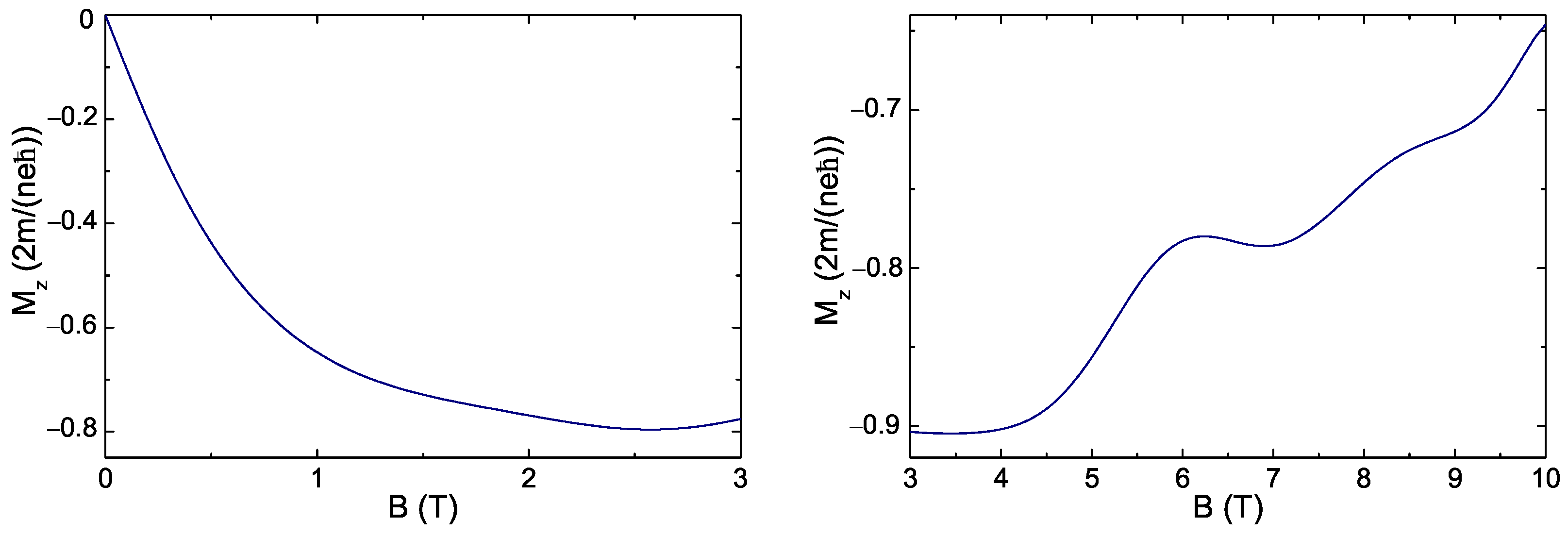
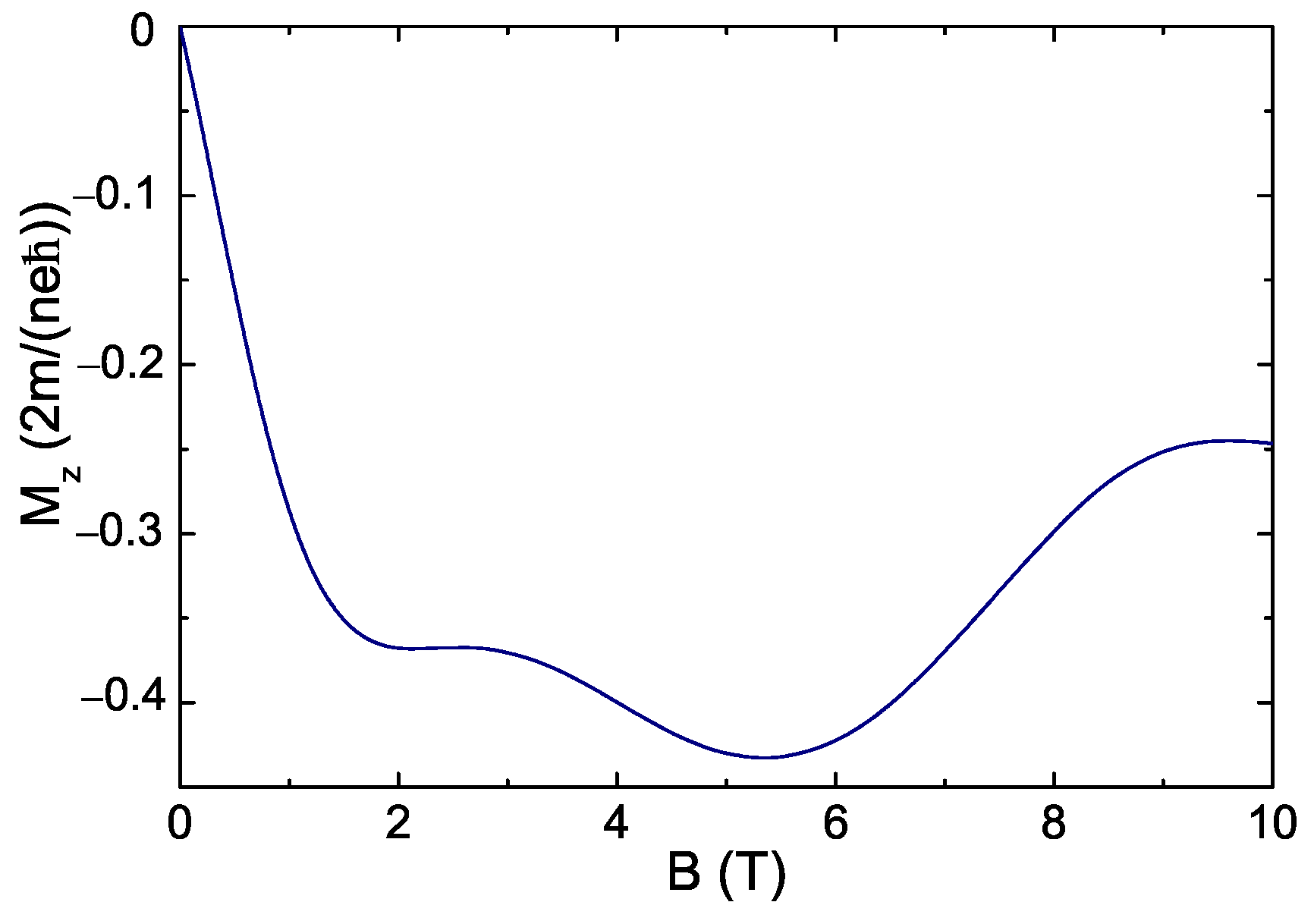
3.2. Magnetization in Graphene

Using Equation (14) and the time-dependent correlations of the random forces, we derive the $z-$component

$$\begin{array}{ccc}\hfill L_z\left(\tau \right)& =& \langle x\left(\tau \right){\pi }_y\left(\tau \right)-y\left(\tau \right){\pi }_x\left(\tau \right)\rangle =\frac{m\hslash {\gamma }^2}{\pi }{\int }_0^{\infty }d\omega {\int }_0^{\tau }dt{\int }_0^{\tau }d{t}^{\prime }\frac{\coth \left[\frac{\hslash \omega }{2T_0}\right]}{{\omega }^2+{\gamma }^2}\cos \left[\omega (t-t^{\prime })\right]\hfill \\ & \times & \{{\lambda }_x\left[B_2\left(t\right)C_1\left(t^{\prime }\right)-A_1\left(t\right)D_2\left(t^{\prime }\right)\right]+{\lambda }_y\left[A_2\left(t\right)D_1\left(t^{\prime }\right)-B_1\left(t\right)C_2\left(t^{\prime }\right)\right]\}\hfill \end{array}$$

(40)

of angular momentum or the magnetization $M\left(\tau \right)=ne{L}_z\left(\tau \right)/\left(2m\right)$. As seen in Figure 15, at weak magnetic fields ($B\le 3$ T), the magnetization $M_z$ in graphene decreases with increasing B without any oscillations. At strong magnetic fields ($B>3$ T), plateau-like structures are observed. Even though the plateaus of $M_z$ are slightly different from the ones of $R_{xy}$ (Figure 2), there is a correlation between them: the Hall resistance $R_{xy}$ is constant but the $|M_z|$ decreases in the interval $B\approx 4-6$ T. In the interval $B\approx 6-7.5$ T, the Hall resistance $R_{xy}$ increases sharply, while $M_z$ remains almost constant (see Figure 2 and Figure 15). Note, that the plateaus appear when $\tau$ is approaching ${\tau }_r$ with increasing B. The dependence of the predicted magnetization $M_z$ on the magnetic field in graphene with the properties as in Figure 7 is shown in Figure 16. The temperature of a sample is relatively high ($T_0=10$ K) and the mobility is relatively small ($\mu =2700$ cm${}^2$V${}^{-1}$s${}^{-1}$); so as a result, the magnetization is small. In Figure 16, plateau-like structures are also formed at $B>1.5$ T when the values of $\tau$ are ${\tau }_r$ are closer to each other.

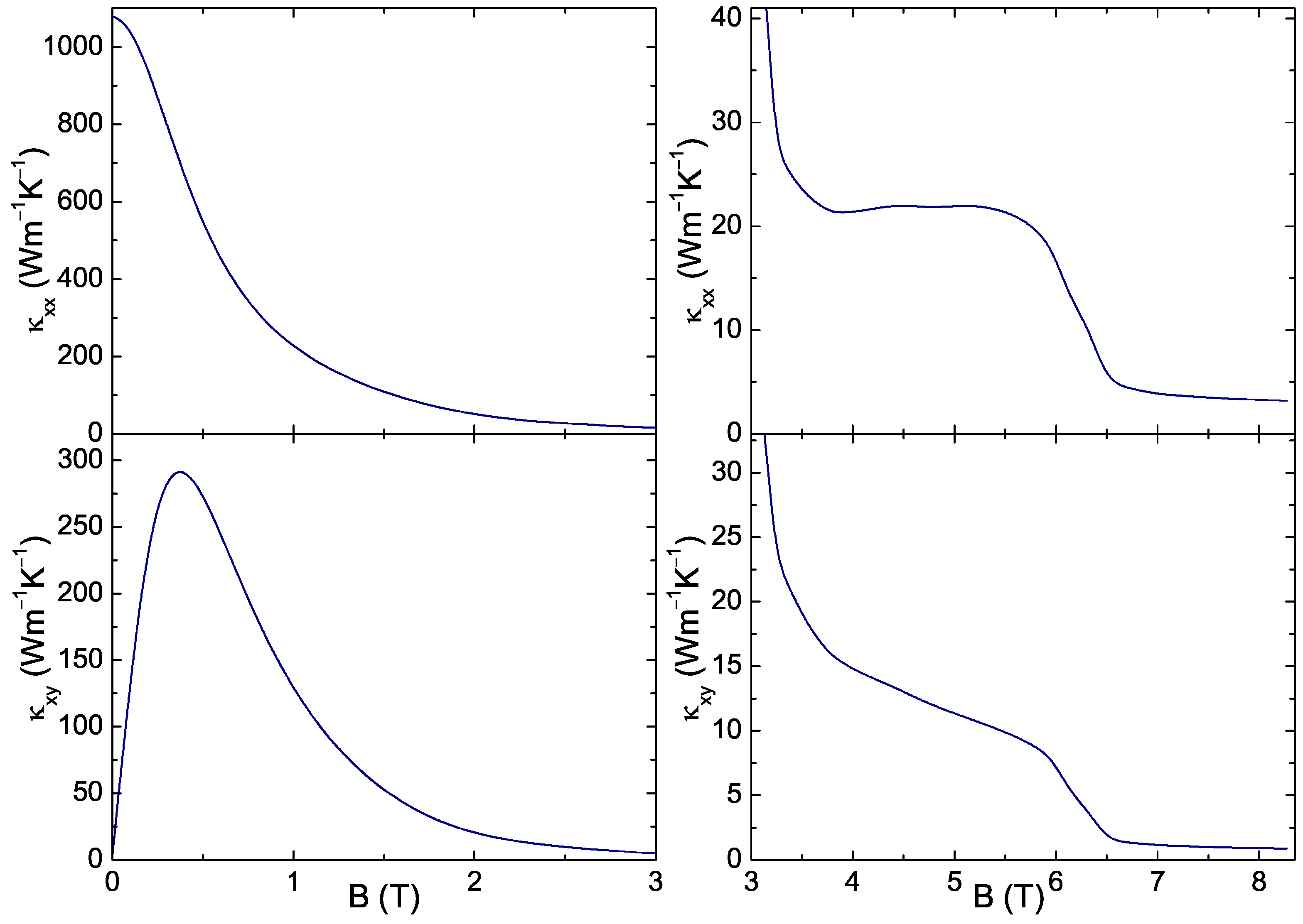
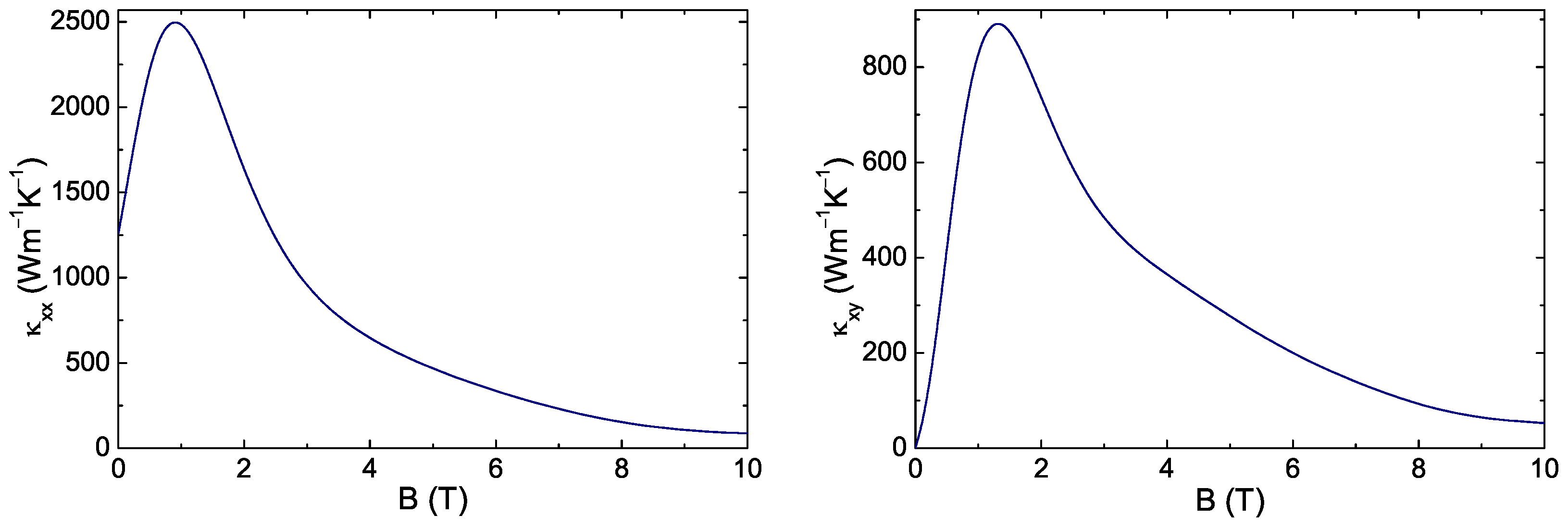
3.3. Thermal Conductivity

We assume the same ability of the carriers to carry a charge and transport heat. If the electric energy gradient $e{E}_x$ in (1) is substituted by the temperature gradient $d{T}_0/dx$ (the temperature is in energy units), the generating force of particle motion changes from electric to thermal potential, giving rise to thermomagnetic effects. Employing the formula

$$\begin{array}{ccc}\hfill \mathbf{Q}& =& n{\epsilon }_{kin}\dot{\mathbf{q}}\hfill \end{array}$$

(41)

for heat flux, the expression for the thermal conductivity tensor is obtained as

$$\begin{array}{ccc}\hfill \kappa \left(\tau \right)& =& \frac{1}{e^2}{\epsilon }_{kin}\left(\tau \right)\sigma \left(\tau \right),\hfill \end{array}$$

(42)

where ${\epsilon }_{kin}$ is the average kinetic energy of the charged particle. In the quasi-equilibrium high-temperature limit ($\tau \to \infty$), one can derive the classical Wiedemann–Franz law [6] for the Lorentz number

$$\begin{array}{ccc}\hfill L& =& \frac{\kappa }{\sigma T_0}=\frac{1}{e^2}=const.\hfill \end{array}$$

(43)

Thus, we obtain a violation of the Wiedemann–Franz law in graphene at low temperatures, which was experimentally observed in ref. [29].

The magnetic field dependencies of the diagonal ${\kappa }_{xx}$ and off-diagonal ${\kappa }_{xy}$ components of the thermal conductivity in graphene at $T_0=$ 30 mK ($m=0.025m_0$, $\mu$ = 13,000 cm${}^2$V${}^{-1}$s${}^{-1}$ [17]) are shown in Figure 17. At weak magnetic fields, ${\kappa }_{xx}$ decreases smoothly with increasing magnetic field. This is more due to the fact that the speed of charge carriers decreases with increasing magnetic field. At $B\approx 0$, the diagonal thermal conductivity is equal to ${\kappa }_{xx}\approx 1000$ Wm${}^{-1}$K${}^{-1}$ and the off-diagonal thermal conductivity is equal to ${\kappa }_{xy}\approx 0$. When ${\upsilon }_y$ reaches its maximum value, ${\kappa }_{xy}$ also reaches its maximum value and then decreases (${\kappa }_{xy}^{max}\approx 300$ Wm${}^{-1}$K${}^{-1}$). If the magnetic field is strong enough ($B\ge 3$ T), a noticeably large plateau-like structure is formed in ${\kappa }_{xx}$.

Figure 18 shows the dependence of the diagonal ${\kappa }_{xx}$ and non-diagonal ${\kappa }_{xy}$ on the magnetic field in graphene ($T_0=10$ K, $m=0.04m_0$, $\mu =2700$ cm${}^2$V${}^{-1}$s${}^{-1}$[19]). The values of $\tau /{\tau }_r$ are taken from Figure 8. It is also clear that ${\kappa }_{xx}>{\kappa }_{xy}$ at weak magnetic fields. Plateau-like behavior is not observed due to the low mobility of the charge carriers.

Note, that the value of the thermal conductivity in graphene at room temperature and $B=0$ ranges from ${\kappa }_{xx}\approx 600$ to 5500 Wm${}^{-1}$K${}^{-1}$[27,28,30]. The calculated ${\kappa }_{xx}$ in Figure 17 and Figure 18 are in the intermediate range shown by the experimental data.

4. Conclusions

Using the non-Markovian quantum Langevin approach and taking into account the coupling between charge carriers and the environment, and two-body effects, we described the SdHO and QHE and predicted thermal conductivity and magnetization in graphene and 2DEG. As shown, the galvano-, and thermo-magnetic effects strongly depend on the relationship between the relaxation and average collision times. The suitable average collision times were adjusted to describe the experimental data. One of the main conclusions of this work is that the values of relaxation and collision times are comparable and, thus, the SdHO and QHE are the results of the transitional processes. As shown for the QHE, the transverse velocity (momentum) is quantized and the transverse current is a step-like function of the magnetic field or charge density. Plateau-like behavior was predicted for the off-diagonal resistance in the SdHO, off-diagonal thermal conductivity, and magnetization in graphene and GaAs/Al${}_x$Ga${}_{1-x}$As heterostructure.

References

1. Geim, A.K. Graphene: Status and Prospects. Science 2009, 324, 1530. [Google Scholar] [CrossRef] [PubMed]
2. Novoselov, K.S. Nobel Lecture: Graphene: Materials in the Flatland. Phys. Mod. Rev. 2011, 83, 837. [Google Scholar] [CrossRef]
3. Castro Neto, A.H.; Guinea, F.; Peres, N.M.R.; Novoselov, K.S.; Geim, A.K. The electronic properties of graphene. Phys. Mod. Rev. 2009, 81, 109. [Google Scholar] [CrossRef]
4. Deng, N.; Tian, H.; Zhang, J.; Jian, J.; Wu, F.; Shen, Y.; Ren, T.-L. Black phosphorus junctions and their electrical and optoelectronic applications. J. Semicond. 2021, 42, 081001. [Google Scholar] [CrossRef]
5. Xue, X.-X.; Meng, H.; Huang, Z.; Feng, Y.; Qi, X. Black phosphorus-based materials for energy storage and electrocatalytic applications. J. Phys. Energy 2021, 3, 042002. [Google Scholar] [CrossRef]
6. Kittel, C. Introduction to Solid State Physics, 8th ed.; John Wiley & Sonc, Inc.: Hoboken, NJ, USA, 2005. [Google Scholar]
7. Komatsubara, K.F. Effect of Electric Field on the Transverse Magnetoresistance in n—Indium Antimonide at 1.5 K. Phys. Rev. Lett. 1966, 16, 1044. [Google Scholar] [CrossRef]
8. Bauer, G.; Kahlert, H. Hot electron Shubnikov–de Haas effect in n-InSb. J. Phys. C Solid State Phys. 1973, 6, 1253. [Google Scholar] [CrossRef]
9. Von Klitzing, K.; Dorda, G.; Pepper, M. New Method for High-Accuracy Determination of the Fine-Structure Constant Based on Quantized Hall Resistance. Phys. Rev. Lett. 1980, 45, 494. [Google Scholar] [CrossRef]
10. Tsui, D.C.; Stormer, H.L.; Gossard, A.C. Two-Dimensional Magnetotransport in the Extreme Quantum Limit. Phys. Rev. B 1982, 48, 1559. [Google Scholar]
11. Willet, R.; Eisenstein, J.P.; Stormer, H.L.; Tsui, D.C.; Gossard, A.C.; English, J.H. Observation of an even-denominator quantum number in the fractional quantum Hall effect. Phys. Rev. Lett. 1987, 59, 1776. [Google Scholar] [CrossRef]
12. Tsui, D.C. Nobel Lecture: Interplay of disorder and interaction in two-dimensional electron gas in intense magnetic fields. Rev. Mod. Phys. 1999, 71, 891. [Google Scholar] [CrossRef]
13. Wei, H.P.; Tsui, D.C.; Paalanen, M.A.; Pruisken, A.M.M. Experiments on Delocalization and University in the Integral Quantum Hall Effect. Phys. Rev. Lett. 1988, 61, 1294. [Google Scholar] [CrossRef] [PubMed]
14. Li, L.; Yang, F.; Ye, G.J.; Zhang, Z.; Zhu, Z.; Lou, W.; Zhou, X.; Li, L.; Watanabe, K.; Taniguchi, T.; et al. Quantum Hall effect in black phosphorus two-dimensional electron system. Nat. Nanotechnol. 2016, 11, 593. [Google Scholar] [CrossRef] [PubMed]
15. Valagiannopoulos, C.A.; Mattheakis, M.; Shirodkar, S.N.; Kaxiras, E. Manipulating polarized light with a planar slab of black phosphorus. J. Phys. Commun. 2017, 1, 045003. [Google Scholar] [CrossRef]
16. Hill, S.; Brooks, J.S.; Uji, S.; Takashita, M.; Terakura, C.; Terashima, T.; Aoki, H.; Fisk, Z.; Sarrao, J. Bulk Quantum Hall Effect In η-Mo4O11. Synth. Matals 1999, 103, 2667. [Google Scholar] [CrossRef]
17. Zhang, Y.; Tan, Y.W.; Stormer, H.L.; Kim, P. Experimental observation of the quantum Hall effect and Berry’s phase in graphene. Nature 2005, 438, 201. [Google Scholar] [CrossRef]
18. Novoselov, K.S.; Giem, A.K.; Morozov, S.V.; Jiang, D.; Zhang, Y.; Dubonos, S.V.; Grigorieva, I.V.; Firsov, A.A. Electric Field Effect in Atomically Thin Carbon Films. Science 2004, 306, 666. [Google Scholar] [CrossRef]
19. Novoselov, K.S.; Geim, A.K.; Morozov, S.V.; Jiang, D.; Katsnelson, M.I.; Grigorieva, I.V.; Dubonos, S.V.; Firsov, A.A. Two-dimensional gas of massless Dirac fermions in graphene. Nature 2005, 438, 197. [Google Scholar] [CrossRef]
20. Novoselov, K.S.; Jiang, Z.; Zhang, Y.; Morozov, S.V.; Stormer, H.L.; Zeitler, U.; Maan, J.C.; Boebinger, G.S.; Kim, P.; Geim, A.K. Room-temperature quantum Hall effect in graphene. Science 2007, 315, 1379. [Google Scholar] [CrossRef]
21. Chen, J.H.; Jang, C.; Xiao, S.; Ishigami, M.; Fuhrer, M.S. Intrinsic and extrinsic performance limits of graphene devices on SiO2. Nat. Nanotechnol. 2008, 3, 206. [Google Scholar] [CrossRef]
22. Du, X.; Skachko, I.; Barker, A.; Andrei, E.Y. Approaching ballistic transport in suspended graphene. Nat. Nanotechnol. 2008, 3, 491. [Google Scholar] [CrossRef] [PubMed]
23. Ezawa, Z.F. Quantum Hall Effects: Field Theoretical Approach and Related Topics; World Scientific: Hackensack, NJ, USA, 2008. [Google Scholar]
24. Cooper, D.R.; D’Anjou, B.; Ghattamaneni, N.; Harack, B.; Hilke, M.; Horth, A.; Majlis, N.; Massicote, M.; Vandsburger, L.; Whiteway, E.; et al. Experimental Review of Graphene. Inter. Sch. Res. Not. Condens. Matter Phys. 2012, 2012, 501686. [Google Scholar] [CrossRef]
25. Aoki, H.; Dresselhaus, M.S. Physics of Graphene; Springer International Publishing: Chem, Switzerland, 2014. [Google Scholar]
26. Katsnelson, M.I. The Physics of Graphene, 2nd ed.; Cambridge University Press: Cambridge, UK, 2020. [Google Scholar]
27. Balandin, A.A. Thermal properties of graphene and nanostructured carbon materials. Nat. Mater. 2011, 10, 569. [Google Scholar] [CrossRef] [PubMed]
28. Pop, E.; Varshney, V.; Roy, A.K. Thermal properties of graphene: Fundamentals and applications. MRS Bull. 2012, 37, 1273. [Google Scholar] [CrossRef]
29. Crossno, J.; Shi, J.K.; Wang, K.; Liu, X.; Harzheim, A.; Lucas, A.; Sachdev, S.; Kim, P.; Taniguchi, T.; Watanabe, K.; et al. Observation of the Dirac fluid and the breakdown of the Wiedemann–Franz law in graphene. Science 2016, 351, 1058. [Google Scholar] [CrossRef] [PubMed]
30. Sang, M.; Shin, J.; Kim, K.; Yu, K.J. Electronic and Thermal Properties of Graphene and Recent Advances in Graphene Based Electronics Applications. Nanomaterials 2019, 9, 374. [Google Scholar] [CrossRef]
31. Ando, T.; Uemura, Y. Theory of Quantum Transport in a Two-Dimensional Electron System under Magnetic Fields. I. Characteristics of Level Broadening and Transport under Strong Fields. J. Phys. Soc. Jpn. 1974, 36, 4. [Google Scholar] [CrossRef]
32. Ando, T. Theory of Quantum Transport in a Two-Dimensional Electron System under Magnetic Fields II. Single-Site Approximation under Strong Fields. J. Phys. Soc. Jpn. 1974, 36, 6. [Google Scholar] [CrossRef]
33. Ando, T. Theory of Quantum Transport in a Two-Dimensional Electron System under Magnetic Fields. III. Many-Site Approximation. J. Phys. Soc. Jpn. 1974, 37, 3. [Google Scholar] [CrossRef]
34. Ando, T. Theory of Quantum Transport in a Two-Dimensional Electron System under Magnetic Fields. IV. Oscillatory Conductivity. J. Phys. Soc. Jpn. 1974, 37, 5. [Google Scholar] [CrossRef]
35. Zheng, Y.; Ando, T. Hall conductivity of a two-dimensional graphite system. Phys. Rev. B 2002, 65, 245420. [Google Scholar] [CrossRef]
36. Van Kampen, N.G. Stochastic Processes in Physics and Chemistry; Elsevier: Amsterdam, The Netherlands, 1981. [Google Scholar]
37. Caldeira, A.O.; Leggett, A.J. Influence of Dissipation on Quantum Tunneling in Macroscopic Systems. Phys. Rev. Lett. 1981, 46, 211. [Google Scholar] [CrossRef]
38. Caldeira, A.O.; Leggett, A.J. Quantum tunnelling in a dissipative system. Ann. Phys. 1983, 149, 374. [Google Scholar] [CrossRef]
39. Lindenberg, K.; West, B.J. The Nonequilibrium Statistical Mechanics of Open and Closed; VCH Publisher: New York, NY, USA, 1990. [Google Scholar]
40. Isar, A.; Sandulescu, A.; Scutaru, H.; Stefanescu, E.; Scheid, W. Open quantum systems. Int. J. Mod. Phys. E 1994, 3, 635. [Google Scholar] [CrossRef]
41. Weiss, U. Quantum Dissipative Systems; World Scientific: Singapore, 1999. [Google Scholar]
42. Kanokov, Z.; Palchikov, Y.V.; Adamian, G.G.; Antonenko, N.V.; Scheid, W. Non-Markovian dynamics of quantum systems. I. Formalism and transport coefficients. Phys. Rev. E 2005, 71, 016121. [Google Scholar] [CrossRef] [PubMed]
43. Kalandarov, S.A.; Abdurakhmanov, I.B.; Kanokov, Z.; Adamian, G.G.; Antonenko, N.V. Angular momentum of open quantum systems in external magnetic field. Phys. Rev. A 2019, 99, 062109. [Google Scholar] [CrossRef]
44. Lacroix, D.; Sargsyan, V.V.; Adamian, G.G.; Antonenko, N.V. Description of non-Markovian effect in open quantum system with the discretized environment method. Eur. Phys. J. B 2015, 88, 89. [Google Scholar] [CrossRef]
45. Alpomishev, E.K.; Adamian, G.G.; Antonenko, N.V. Orbital diamagnetism of two-dimensional quantum systems in a dissipative environment: Non-Markovian effect and application to graphene. Phys. Rev. E 2021, 104, 054120. [Google Scholar] [CrossRef]
46. Abdurakhmanov, I.B.; Kanokov, Z.; Adamian, G.G.; Antonenko, N.V. Galvano- and thermo-magnetic effects at low and high temperatures within non-Markovian quantum Langevin approach. Phys. A 2018, 508, 613. [Google Scholar] [CrossRef]
47. Van Wees, B.J.; van Houten, H.; Beenakker, C.W.J.; Williamson, J.G.; Kouwenhoven, L.P.; van der Marel, D.; Foxon, C.T. Quantized conductance of point contacts in a two-dimensional electron gas. Phys. Rev. Lett. 1988, 60, 848. [Google Scholar] [CrossRef]
48. Wharam, D.A.; Thornton, T.J.; Newbury, R.; Pepper, M.; Ahmed, H.; Frost, J.E.F.; Hasco, D.G.; Peacock, D.C.; Ritchie, D.A.; Jones, G.A. One-dimensional transport and the quantisation of the ballistic resistance. J. Phys. C Sol. St. Phys. 1988, 21, L209. [Google Scholar] [CrossRef]
49. Tombros, N.; Veligura, A.; Junesch, J.; Gumarães, H.D.; Vera-Marun, I.J.; Jonkman, H.T.; van Wees, B.J. Quantized conductance of a suspended graphene nanoconstriction. Nat. Phys. 2011, 7, 697. [Google Scholar] [CrossRef]
50. Kirczenow, G. Hall effect and ballistic conduction of in a two-dimensional quantum wires. Phys. Rev. B 1988, 38, 10958. [Google Scholar] [CrossRef] [PubMed]
Figure 1. Schematic illustration of the motion (time arrow t indicated) of the charge carrier (small green circle) between two successive collisions with ions/atoms (large brown circles) of the lattice as well as the relaxation time τ r and the average collision time τ scales in 2D magnetotransport. Uniform magnetic field B = ( 0 , 0 , B ) perpendicular to the x y plane (along the z-axis), and the constant electric field E = ( E x , 0 , 0 ) acts in the direction of the x-axis.
Symmetry 16 00007 g001
Figure 2. Dependencies of R x x (left side) and R x y (right side) on the magnetic field B. Experimental results (solid lines) are taken from ref. [17]. Here, the charge carrier mobility is μ = 13,000 cm 2 V 1 s 1 , gate voltage V g = 15 V, and temperature of graphene T 0 = 30 mK.
Symmetry 16 00007 g002
Figure 3. The dependence of τ / τ r , extracted from the experimental data of ref. [17], on the magnetic field B.
Symmetry 16 00007 g003
Figure 4. The dependence of υ / c on the magnetic field B.
Symmetry 16 00007 g004
Figure 5. For the SdHO, the longitudinal resistivity resistance (the left plot) and the predicted Hall resistance (the right plot) in graphene at different temperatures and magnetic fields. Experimental data (solid lines) are taken from ref. [17]. Here the charge carrier mobility in graphene is μ = 15,000 cm 2 V 1 s 1 .
Symmetry 16 00007 g005
Figure 6. The calculated oscillation part of the Hall resistance ( Δ R x y ) and τ / τ r at different temperatures and magnetic fields.
Symmetry 16 00007 g006
Figure 7. The SdHO (left) and the oscillation part Δ R x y of the Hall resistance (right). Experimental results (solid line) are taken from ref. [19]. Here, the charge carrier mobility of graphene is μ = 2700 cm 2 V 1 s 1 , carrier density n = 4.38 × 10 12 cm 2 , and temperature T 0 = 10 K. The predicted Hall resistance is shown inside.
Symmetry 16 00007 g007
Figure 8. The dependencies of τ / τ r , extracted from the experimental data of ref. [19], on the magnetic field B.
Symmetry 16 00007 g008
Figure 9. Resistivity R x x and Hall conductivity σ x y as a function of the carrier density n. Experimental results (solid lines) are taken from ref. [19]. Here, the magnetic field is B = 14 T and temperature T 0 = 4 K.
Symmetry 16 00007 g009
Figure 10. The dependence of τ / τ r on the carrier density n.
Symmetry 16 00007 g010
Figure 11. Dependencies of longitudinal υ x and transverse υ y velocities on the carrier density n.
Symmetry 16 00007 g011
Figure 12. The dependence of the transverse current density J y on the carrier density n.
Symmetry 16 00007 g012
Figure 13. Dependencies of R x x (left) and R x y (right) on B in 2DEG. Experimental data (solid lines) are taken from ref. [12]. Here the charge carrier mobility is μ = 52,000 cm 2 V 1 s 1 , carrier density n = 1.93 × 10 11 cm 2 , and temperature T 0 = 66 mK.
Symmetry 16 00007 g013
Figure 14. The dependence of τ / τ r on B (left) for 2DEG [12]. The values of τ / τ r for graphene (dashed lines) [17] and 2DEG (solid lines) [12] are compared (right). Here, the charge carrier mobility in graphene is μ = 13,000 cm 2 V 1 s 1 and temperature T 0 = 30 mK [17]. The charge carrier mobility in 2DEG is μ = 52,000 cm 2 V 1 s 1 and temperature T 0 = 66 mK.
Symmetry 16 00007 g014
Figure 15. The dependence of magnetization M z on the magnetic field in graphene at T 0 = 30 mK ( m = 0.025 m 0 ( m 0 is the bare mass of an electron), μ = 13,000 cm 2 V 1 s 1 [17]).
Symmetry 16 00007 g015
Figure 16. The dependence of magnetization M z on the magnetic field in graphene at T 0 = 10 K ( m = 0.04 m 0 , μ = 2700 cm 2 V 1 s 1 [19]).
Symmetry 16 00007 g016
Figure 17. The dependencies of the diagonal κ x x and non-diagonal κ x y components of the thermal conductivity on the magnetic field at T 0 = 30 mK ( μ = 13,000 cm 2 V 1 s 1 [17]).
Symmetry 16 00007 g017
Figure 18. The dependencies of the diagonal κ x x and non-diagonal κ x y thermal conductivities on the magnetic field in graphene at T 0 = 10 K ( μ = 2700 cm 2 V 1 s 1 [19]).
Symmetry 16 00007 g018
Disclaimer/Publisher’s Note: The statements, opinions and data contained in all publications are solely those of the individual author(s) and contributor(s) and not of MDPI and/or the editor(s). MDPI and/or the editor(s) disclaim responsibility for any injury to people or property resulting from any ideas, methods, instructions or products referred to in the content.