de Broglie, General Covariance and a Geometric Background to Quantum Mechanics

Abstract

What is striking about de Broglie’s foundational work on wave–particle dualism is the role played by pseudo-Riemannian geometry in his early thinking. While exploring a fully covariant description of the Klein–Gordon equation, he was led to the revolutionary idea that a variable rest mass was essential. DeWitt later explained that in order to obtain a covariant quantum Hamiltonian, one must supplement the classical Hamiltonian with an additional energy ${\hslash }^2\mathcal{Q}$ from which the quantum potential emerges, a potential that Berry has recently shown also arises in classical wave optics. In this paper, we show how these ideas emerge from an essentially geometric structure in which the information normally carried by the wave function is contained within the algebraic description of the geometry itself, within an element of a minimal left ideal. We establish the fundamental importance of conformal symmetry, in which rescaling of the rest mass plays a vital role. Thus, we have the basis for a radically new theory of quantum phenomena based on the process of mass-energy flow.

1. Introduction

One hundred years after de Broglie first suggested that all matter has both wave and particle properties, the physics community is still trying to accommodate these two very different concepts into a fully coherent physical and mathematical picture. Yes, we have learned to live with certain uncomfortable features by developing some ingenious notions to accommodate them. One way or another, these strategies have enabled us to develop outstanding technologies that show we are on the right track.

However the precise nature of the ontology underlying the phenomena is still, at times, under heated debate. The fact that gravity resists inclusion into the quantum formalism indicates that much thinking still has to be done. It is appropriate to stand back from our immediate detailed work and review the overall development of our understanding to date. What better way to achieve this than to revisit de Broglie’s own pioneering work on its 100 year anniversary?

The renascence of the pilot wave model over recent years is well known. Perhaps what is not so familiar is the mathematical and physical motivation lying behind de Broglie’s early work on what he called the “Double Solution”. What struck us upon revisiting de Broglie’s publications was the extent that relativity, both special and general, played in his thinking. Rather than relying solely on the guidance of the classical Hamilton–Jacobi theory in Euclidean geometry, de Broglie was exploring its consequences in a Riemannian geometry.

This becomes quite clear if we look at the appendix to the English translation of de Broglie’s original 1927 paper [1] published in Selected Papers on Wave Mechanics [2] and in a footnote that appears in the English translation of his 1956 book Non-linear Wave Mechanics: a Causal Interpretation [3]. It is the projection of the relativistic structure into a Euclidean space that gives rise to the pilot wave model.

Note that de Broglie himself calls the pilot wave theory “an incomplete and diluted form” [3] of what he had in mind for the Double Solution. His presentation of the simplified pilot wave model to the 1927 Solvay Congress was not well received. After the Congress, de Broglie explained, “I thought over the pilot-wave theory I had maintained, I became aware that it could not really furnish a concrete picture, in conformity with the conceptions of the older Physics, of wave-particle dualism” [3]. As a consequence, de Broglie abandoned his approach and was content to follow the Bohr school.

Bohm’s paper on “hidden variables” [4] changed all of that, as he and de Broglie tried, with Vigier, to apply his ideas to the Dirac particle, unfortunately without much success. Two summers ago, we happened upon a long-forgotten paper by Bryce DeWitt [5] which, remarkably, appeared in the same volume of Physical Review as David Bohm’s “hidden variable” paper [4] but two issues later. While Bohm discussed the “quantum potential” in a Euclidean space, DeWitt explained how this potential arises in the context of a pseudo-Riemannian space.

What DeWitt showed was that the quantum Hamiltonian must contain an extra energy term, ${\hslash }^2\mathcal{Q}$, in order to maintain the principle of general covariance, which is regarded as a key feature of relativity. de Broglie had already found this extra energy term in his 1927 paper [1]. However, de Broglie had actually gone further by bringing in a variable, rest mass, that led him to later show that conformal rescaling [6] was involved. This drew attention to the important role that could be played by the conformal group (The variable rest mass introduced by de Broglie ensures conformal covariance and is associated with the acceleration transformations of the 15 parameter conformal group). In this paper, we will explore some aspects of conformal rescaling in detail. We will also discuss the role of the “quantum” potential, as its appearance has caused much debate. Moreover, we will show that this potential arises as a natural consequence of non-inertial motion and is not exclusive to the quantum domain.

2. The Klein–Gordon Equation in Riemannian Geometry According to de Broglie

We begin by recalling the content of the appendix that de Broglie added in English to his 1927 paper entitled “The Wave Mechanics and the Atomic Structure of Matter and Radiation” [2]. Consider the usual Klein–Gordon equation with a rest mass $m_0$:

$$\begin{array}{c}\hfill \square \Psi +m_0^2\Psi =0\end{array}$$

where □ is the d’Alembertian. To write the Klein–Gordon equation in a pseudo-Riemannian space, we must convert the Minkowski metric into a general metric ${\eta }_{\mu \nu }\to g_{\mu \nu }$ so that the partial derivative can be replaced by the covariant derivative ${\partial }_{\mu }\to {\nabla }_{\mu }$. Then, by writing the d’Alembertian in the general form

$$\begin{array}{c}\hfill \frac{1}{\sqrt{-g}}\frac{\partial }{\partial x^{\mu }}\sqrt{-g}{g}^{\mu \nu }\frac{\partial }{\partial x^{\nu }}\end{array}$$

one obtains the Klein–Gordon equation in tensorial form:

$$\begin{array}{c}\hfill {\nabla }^{\mu }{\nabla }_{\mu }\Psi +M_0^2\Psi =0\end{array}$$

where de Broglie attributes the variable rest mass $M_0$ to the particle. If we now write the real part of the Klein–Gordon equation under polar decomposition of the wave function $\Psi =A{e}^{i\varphi /\hslash }$, we find

$$\begin{array}{c}\hfill \left[g^{\mu \nu }\frac{\partial \varphi }{\partial x^{\mu }}\frac{\partial \varphi }{\partial x^{\nu }}\right]A-{\hslash }^2\square A-m_0^2{c}^{2}A=0\end{array}$$

which can be written in the form

$$\begin{array}{c}\hfill \left[g^{\mu \nu }\frac{\partial \varphi }{\partial x^{\mu }}\frac{\partial \varphi }{\partial x^{\nu }}\right]A-M_0^2{c}^{2}A=0\end{array}$$

where

$$\begin{array}{c}\hfill M_0^2=m_0^2+\frac{{\hslash }^2}{c^2}\left(\frac{\square A}{A}\right).\end{array}$$

In the Newtonian approximation, we have

$$\begin{array}{c}\hfill Q=-\frac{{\hslash }^2}{2m_0}\frac{{\nabla }^{2}A}{A}\end{array}$$

which is the quantum potential that appears in the real part of the non-relativistic Schrödinger equation under polar decomposition of the wave function, as shown in the work of Bohm [4]. Thus, the quantum potential arises as a non-relativistic limit of the variable rest mass [7].

The imaginary part of the Klein–Gordon equation under polar decomposition of the wave function is

$$\begin{array}{c}\hfill \frac{1}{\sqrt{-g}}\frac{\partial }{\partial x^{\mu }}\left[\sqrt{-g}{g}^{\mu \nu }{A}^2\frac{\partial \varphi }{\partial x^{\nu }}\right]=0\end{array}$$

which is just a continuity of the mass-density equation. In the non-relativistic limit, this becomes

$$\begin{array}{c}\hfill {\partial }_t\rho +\nabla .(\rho \nabla \varphi /m)=0.\end{array}$$

We have written $\Psi {\left(\mathit{x}\right)}^{*}\Psi \left(\mathit{x}\right)=\rho \left(\mathit{x}\right)$ and interpreted $\rho$ as the mass-density. Hence in the non-relativistic limit below the particle-antiparticle creation threshold, $\rho \left(\mathit{x}\right)$ can be reinterpreted as the probability of finding a particle at the point $\mathit{x}$ in space. In this approach, we see that the Born probability rule emerges from the non-relativistic conservation of the flow of mass-density when the particle number is conserved. As is well known, the Born probability rule cannot be used in Riemannian space for the Klein–Gordon equation, owing to the appearance of negative probabilities.

2.1. de Broglie’s Introduction of the Conformal Group

It was noted by de Broglie [3] that in Euclidean spacetime with the metric $d{s}^2=g_{\mu \nu }^{\left(0\right)}d{x}^{\mu }d{x}^{\nu }$, in the absence of any electromagnetic or gravitational fields, the principle of least action can be written as

$$\begin{array}{c}\hfill \delta \int d{x}^i{M}_{0}c{u}_i=c\delta \int ds{M}_0=0\end{array}$$

where the integral is taken along the world line and there is no variation in its end points. A set of similar geodesics will be obtained from the variation

$$\begin{array}{c}\hfill c\delta \int d\sigma m_0=0\end{array}$$

by choosing a different coordinate system characterized by a different metric $d{\sigma }^2$. Clearly, the transformation is a conformal one with $d{\sigma }^2={\Omega }^{2}d{s}^2$, where $\Omega =M_0/m_0$. Then, we have

$$\begin{array}{c}\hfill d{\sigma }^2=\frac{M_0^2}{m_0^2}d{s}^2=\frac{M_0^2}{m_0^2}{g}_{\mu \nu }^{\left(0\right)}d{x}^{\mu }d{x}^{\nu }={\gamma }_{\mu \nu }d{x}^{\mu }d{x}^{\nu }\end{array}$$

leading to the expression

$$\begin{array}{c}\hfill {\gamma }_{\mu \nu }=\left(1+\frac{{\hslash }^2}{m_0^2{c}^2}\frac{\square A}{A}\right)g_{\mu \nu }^{\left(0\right)}.\end{array}$$

We therefore see that the “quantum” potential arises directly from the metric structure used to describe the spacetime. In this sense, it is like a gravitational field since a judicious choice of coordinates can reduce it to zero and, as we will show, such forces arise whenever acceleration occurs.

2.2. The Schrödinger Equation According to DeWitt

Now let us return to the neglected paper by Bryce DeWitt [5] and see how he introduces the quantum potential. In the paper, he exploited the isomorphism that exists between the group of point transformations in classical mechanics and a certain subgroup of the unitary transformations used in quantum mechanics. Although not named by DeWitt, this group is the metaplectic group, a group that appears in wave optics [8]. This supplied a method for constructing quantum analogues of classical models which remain covariant under general coordinate transformations.

One of the key steps in the DeWitt paper was to point out that in a pseudo-Riemannian space, the momentum operator ${\widehat{p}}_{\mu }=-i\hslash \partial /\partial x^{\mu }$ must be replaced by

$$\begin{array}{c}\hfill {\widehat{p}}_{\mu }=-i\hslash \frac{\partial }{\partial x^{\mu }}-\frac{1}{2}i\hslash \left\{\begin{array}{c}\kappa \\ \kappa \mu \end{array}\right\}\left(x\right)\end{array}$$

where $\left\{\begin{array}{c}\kappa \\ \kappa \mu \end{array}\right\}$ represents the Christoffel symbols introduced by DeWitt. As a consequence, the quantum analogue of the Hamiltonian must be replaced by

$$\begin{array}{c}\hfill H_q=\frac{1}{2m}{p}_i{g}^{ij}{p}_j+{\hslash }^2\mathcal{Q}+V\end{array}$$

(1)

where

$$\begin{array}{c}\hfill \mathcal{Q}=\frac{1}{4m}{g}^{\mu \nu }\left[{\left\{\begin{array}{c}\kappa \\ \kappa \mu \end{array}\right\}}_{,\nu }-\left\{\begin{array}{c}\kappa \\ \mu \nu \end{array}\right\}\left\{\begin{array}{c}\lambda \\ \lambda \kappa \end{array}\right\}-\frac{1}{2}\left\{\begin{array}{c}\kappa \\ \kappa \mu \end{array}\right\}\left\{\begin{array}{c}\lambda \\ \lambda \nu \end{array}\right\}\right].\end{array}$$

Thus, general covariance demands an additional energy term ${\hslash }^2\mathcal{Q}$, which also appears in Bohm’s 1952 paper [4], albeit in a different form. Both authors refer to it as the “quantum potential”. DeWitt [5] wrote the following:

The quantity ${\hslash }^2\mathcal{Q}$ may be regarded as a kind of quantum mechanical potential which goes to zero, as $\hslash \to 0$. It is the quantity, which must be added to the covariant classical Hamiltonian in order to produce the covariant quantum Hamiltonian.

It is interesting to note that in this paper, DeWitt also applies the quantum formalism to a spherically curved space.

In a later paper, DeWitt [9] showed that $\mathcal{Q}=-\frac{1}{6}\rho \mathcal{R}$, where $\mathcal{R}$ is the Ricci scalar curvature. In summarizing the results, we have

$$\begin{array}{c}\hfill H_q=H_c-\frac{{\hslash }^2}{2m_0}\mathcal{R}/6\to M_0=m_0-\frac{{\hslash }^2}{2m_0{c}^2}\mathcal{R}/6\to M_0^2=m_0^2+\frac{{\hslash }^2}{c^2}\left(\frac{\square A}{A}\right).\end{array}$$

Thus, we see that not only does the wave function become coupled to the rest mass through the quantum potential, but it also becomes coupled to the scalar curvature.

We would like to point out the following historical fact reported by Schulman [10]: DeWitt’s result showing the appearance of a Ricci scalar curvature term was noted at the time, and the feasibility of measuring it was discussed by DeWitt, Wheeler and possibly Feynman, who concluded that it was too small to be detected by the means then available.

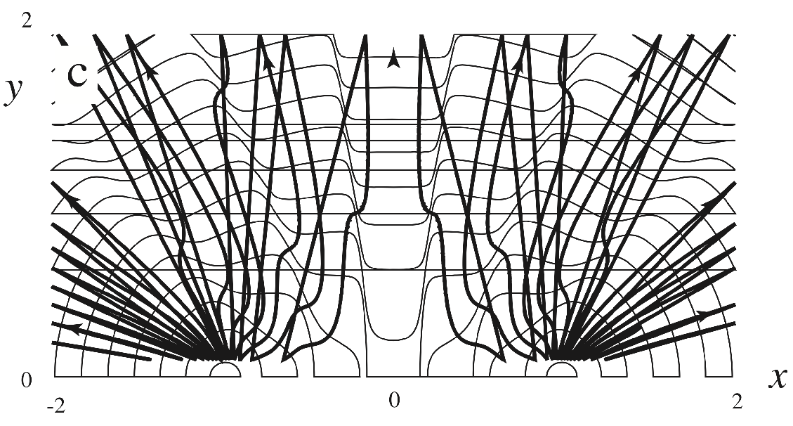
2.3. The Appearance of Curvature in Classical Wave Optics

In 2013, Berry [11] showed that one could construct streamlines of an optical scalar wave field $\psi \left(\mathit{r}\right)$ which satisfy the Helmholtz equation

$$\begin{array}{c}\hfill {\nabla }^2\psi \left(\mathit{r}\right)+B\left(\mathit{r}\right)\psi \left(\mathit{r}\right)=0.\end{array}$$

(2)

Note that in this section, we will use the Berry notation and write ∇ for the three-dimensional symbol for grad. Again, by writing the scalar wave field in polar form $\psi \left(\mathit{r}\right)=A\left(\mathit{r}\right)exp\left[i\chi \right(\mathit{r}\left)\right]$, we can introduce a wave vector field defined by $\mathit{k}\left(\mathit{r}\right)=\nabla \chi \left(\mathit{r}\right)$. This field is tangent to the streamlines emanating from two coherent sources, as shown in Figure 1. Berry [11,12] showed that the curvature vector of the streamlines is given by

$$\begin{array}{c}\hfill \mathit{C}\left(\mathit{r}\right)=\frac{1}{k{\left(\mathit{r}\right)}^2}{\left[(k\left(\mathit{r}\right).\nabla )k\left(\mathit{r}\right)\right]}_{\perp }.\end{array}$$

The real part of the Helmholtz equation is the eikonal equation:

$$\begin{array}{c}\hfill {(\nabla \chi )}^2-n^2=0\end{array}$$

where n is the refractive index of the medium which appears when writing $B\left(\mathit{r}\right)=k_0^2{n}^2\left(\mathit{r}\right)$ ($k_0$ is the vacuum wavenumber). Moreover, the curvature vector of the streamlines may be written in the form

$$\begin{array}{c}\hfill \mathit{C}\left(\mathit{r}\right)=-\frac{1}{2k{\left(\mathit{r}\right)}^2}{\nabla }_{\perp }\left(B\left(\mathit{r}\right)+\frac{{\nabla }^{2}A\left(\mathit{r}\right)}{A\left(\mathit{r}\right)}\right).\end{array}$$

In this way, we see the non-relativistic “quantum” potential appearing in the expression for the curvature vector of classical streamlines.

The time-independent Schrodinger equation can be written in the form of the Helmholtz equation (Equation (2)), provided we identify

$$\begin{array}{c}\hfill B\left(\mathit{r}\right)=\frac{2m}{{\hslash }^2}(E-V\left(\mathit{r}\right)).\end{array}$$

“Quantum streamlines”, called “trajectories”, have been calculated from the Schrodinger equation by Philippidis, Dewdney and Hiley [13]. These results directly connect the scalar curvature (given by the curvature vector’s magnitude) with momentum flow-lines in general.

For completeness, before leaving this topic, we remind the reader of the motion of a particle of mass $m_1$ rotating in a gravitational central potential generated by a second particle of mass $m_2$. Here, the Lagrangian is

$$\begin{array}{c}\hfill \mathcal{L}=-\mu c^2\gamma -V\left(\mathit{r}\right)\mathrm{where}\gamma ={\left[1-\frac{{\dot{r}}^2+r^2{\dot{\theta }}^2}{c^2}\right]}^{1/2}\end{array}$$

where $\mu$ is the reduced mass:

$$\begin{array}{c}\hfill \frac{1}{\mu }=\frac{1}{m_1}+\frac{1}{m_2}.\end{array}$$

The classical Euler–Lagrange equation then becomes

$$\begin{array}{c}\hfill d\left(\gamma \dot{\mathit{r}}\right)/dt-\gamma \mathit{r}{\dot{\theta }}^2+\mathit{F}/\mu =0\mathrm{where}\mathit{F}=-\partial V/\partial \mathit{r}\end{array}$$

(3)

showing that as well as the radial kinetic energy, there is a rotational energy term: a Coriolis term. This follows from the fact that, in general, the conservation of energy equation must contain terms involving linear kinetic energy together with rotational kinetic energy, and thus we have

$$\begin{array}{c}\hfill \frac{\mu {\dot{r}}^2}{2}+\frac{L^2}{2\mu r^2}+V\left(\mathit{r}\right)=E\end{array}$$

where L is the angular momentum. The appearance of angular momentum means that the analogue of the $B\left(\mathit{r}\right)$ term in the Helmholtz equation must have the form

$$\begin{array}{c}\hfill B\left(\mathit{r}\right)=\frac{2}{\mu }\left(E-V\left(\mathit{r}\right)-\frac{L^2}{2\mu r^2}\right).\end{array}$$

Now when comparing this with the results of Berry’s work, we see that the “quantum” potential energy arises from a term featuring the angular momentum. This term involves any deviation from a straight flow line and therefore must give rise to a Coriolis effect. Hence, as a flow line begins to turn, there is a transfer of translational energy into rotational energy, ensuring energy is conserved. This has a consequence for quantum mechanics, which we will now discuss in detail.

2.4. The Appearance of a Complex Field in Quantum Mechanics

Before beginning this discussion, we draw attention to Heisenberg’s [14] criticism of the de Broglie–Bohm pilot wave model, where he claimed there is a need to introduce some strange “ad hoc quantum potentials”. However, Heisenberg ([14], p. 116.) himself advocated for the use of a Lagrangian written in the form

$$\begin{array}{c}\hfill \mathcal{L}=-\frac{{\hslash }^2}{2m}\nabla {\psi }^{*}·\nabla \psi +\frac{i\hslash }{2}[{\psi }^{*}\left({\partial }_t\psi \right)-\left({\partial }_t{\psi }^{*}\right)\psi ]-V{\psi }^{*}\psi \end{array}$$

(4)

from which he obtains the Schrödinger equation and its dual. Let us now put the polar form of the wave function, written here as $\psi =R{e}^{iS/\hslash }$, in the Lagrangian (Equation (4)) so that it becomes

$$\begin{array}{c}\hfill \mathcal{L}=-R^2\left({\partial }_{t}S+\frac{{(\nabla S)}^2}{2m}+\frac{{\hslash }^2}{2m}\frac{{(\nabla R)}^2}{R^2}+V\right).\end{array}$$

If we now treat R and S as independent real variables and derive the Euler–Lagrange equations in the usual way, we obtain two equations. The first is

$$\begin{array}{c}\hfill {\partial }_t\rho +\nabla .(\rho \nabla S/m)=0\end{array}$$

which is just the Bohm equation for the conservation of probability. The second is the Bohm quantum Hamilton–Jacobi equation, which expresses the conservation of energy:

$$\begin{array}{c}\hfill {\partial }_{t}S+\frac{{(\nabla S)}^2}{2m}-\frac{{\hslash }^2}{2m}\frac{{\nabla }^{2}R}{R}+V=0.\end{array}$$

(5)

We see the quantum potential arising in this equation not as an ad hoc term but as a necessary consequence of writing the wave function in polar form. Notice further that it appears including ${\hslash }^2$ in exactly the way that DeWitt claimed was needed in order to satisfy the principle of general covariance. Of course, this does not explain why the quantum potential arises. We have to carry out a lot more work before we can uncover the reason for it being there.

To accomplish this, we need to discuss the role of the metric tensor in Riemannian quantum mechanics. First notice that two types of momenta appear in Equation (5). One has been called the Bohm momentum $p_B=\nabla S$, and the other has been called the “osmotic” momentum, with the term “osmotic” arising for historical reasons, as it first appeared in Nelson’s [15] work when he tried to generate the Schrödinger equation from a stochastic model of underlying mechanics. In our approach, the “osmotic” momentum takes the form $\hslash \nabla R/R$, indicating that it arises from the amplitude of the wave function, as does the “quantum” potential. Once again, this shows that the amplitude of the wave function is playing a direct role in the dynamics.

Beautiful examples illustrating the roles played by both momenta can be found in the work of Bliokh et al. [16], where two different physical situations are explored: the two-slit interference experiment and a particle being “floated” on an intense, circularly polarized beam of laser light. This latter experimental example clearly demonstrates the Coriolis effect arising directly from the “osmotic” term.

2.5. Combining the Two Real Momenta into One Complex Momentum

Thus far, we have seen that when analyzing the quantum formalism in Riemannian geometry, novel features appear. In order to obtain a better understanding of these features, we will approach the differential geometry from Synge’s perspective [17] by introducing a two-point world function $W(x,x^{\prime })$ and studying its coincident limit $W(x,x^{\prime })\to W_c\left(x\right)$.

To prepare the ground, let us first introduce a generalized momentum $\mathit{P}(\mathit{r},t)=-i\nabla ln\psi (\mathit{r},t)$ so that when we write $\psi (\mathit{r},t)=A(\mathit{r},t)e^{iS(\mathit{r},t)}$, with $\hslash =1$, we find

$$\begin{array}{c}\hfill \mathit{P}(\mathit{r},t)=\nabla S(\mathit{r},t)-i\nabla lnA(\mathit{r},t).\end{array}$$

At first sight, the appearance of complex momentum in a differential geometry setting is a bit puzzling. However, if we treat i as an “action” in the Clifford sense rather than a “number” in the real field sense, then we can interpret $\nabla S$ and $\nabla lnA$ as acting at right angles to each other. But this is exactly what we want, because we may then interpret $\nabla S$ as the tangent momentum to the trajectory, while $\nabla lnA$ is the perpendicular momentum. It is the behavior of this perpendicular momentum that is used to calculate the curvature of the trajectory. This then provides a simple explanation of the Berry [11] result discussed in Section 2.3. It also explains the appearance of the Ricci scalar curvature. Let us put this side of the argument on hold temporarily and see how the idea can be used in Riemannian geometry.

2.6. The Role of the Metric Tensor

In Riemannian geometry, different qualities of energy can emerge from the elements of the metric tensor. To see how this happens, let us consider how geodesics are expressed in more formal terms. This means writing the Euler–Lagrange equations (Equation (3)) in a generalized form:

$$\begin{array}{c}\hfill \left(\frac{d{u}^{\mu }}{ds}\right)-\left\{\begin{array}{c}\mu \beta \\ \alpha \end{array}\right\}\left(u_{\alpha }{u}^{\beta }\right)-{\mathcal{F}}^{\mu }/\rho =0\end{array}$$

where $\rho$ is the mass-density, $u^{\mu }=d{x}^{\mu }/ds$ is the four velocity with $u_{\mu }{u}^{\mu }=1$ and ${\mathcal{F}}^{\mu }$ is the externally applied force. Weyl [18] wrote this equation in the form

$$\begin{array}{c}\hfill \rho \left(\frac{d{u}^{\mu }}{ds}\right)-{\overline{\mathcal{F}}}^{\mu }-{\mathcal{F}}^{\mu }=0\end{array}$$

where ${\overline{\mathcal{F}}}^{\mu }$ is regarded as a “pseudo-force”, of which the Coriolis force is a simple example.

For a first approximation, we may write

$$\begin{array}{c}\hfill \frac{d{x}^0}{ds}\simeq 1,\frac{d{x}^1}{ds}\simeq \frac{d{x}^2}{ds}\simeq \frac{d{x}^3}{ds}\simeq 0.\end{array}$$

Then, with the metric $d{s}^2=g_{\mu \nu }d{x}^{\mu }d{x}^{\nu }$, the geodesic equation simply becomes

$$\begin{array}{c}\hfill \left(\frac{d^2{x}^{\mu }}{d{\left(x^0\right)}^2}\right)-\frac{1}{2}\frac{\partial g_{00}}{\partial x^{\mu }}=0.\end{array}$$

In a rotating frame where $\theta ={\theta }^{\prime }+\omega t^{\prime }$ and $t=t^{\prime }$, the Euclidean metric

$$\begin{array}{c}\hfill d{s}^2=d{t}^2-(d{z}^2+d{r}^2+r^{2}d{\theta }^2)\end{array}$$

becomes

$$\begin{array}{c}\hfill d{s}^2=d{t}^2(1-r^2{\omega }^2)-2r^2\omega d\theta dt-(d{z}^2+d{r}^2+r^{2}d{\theta }^2).\end{array}$$

Following Weyl [18], we have $u^1=u^2=u^3=0,\mathrm{with}{\left(u^0\right)}^2(1-r^2{\omega }^2)=1$. If we now change the variables to $t=x_0,\theta =x^1,z=x^2$ and $r=x^3$, we then find that the forces acting on the flow are

$$\begin{array}{c}\hfill {\overline{\mathcal{F}}}_3=\frac{1}{2}\frac{\partial g_{00}}{\partial x^3}.\rho {\left(u^0\right)}^2=-r{\omega }^2\rho {\left(u^0\right)}^2\mathrm{and}{\overline{\mathcal{F}}}_0={\overline{\mathcal{F}}}_1={\overline{\mathcal{F}}}_2=0.\end{array}$$

In this way, we show $\partial g_{00}/\partial x^3=-2r{\dot{\theta }}^2$, and thus the Coriolis term is already encoded in the metric.

As an aside, we remark that in polyatomic molecules, the vibrational energies of the bonds change when the molecules are rotating [19]. We therefore find experimental evidence of the Coriolis effect in molecular spectra.

2.7. The Appearance of the Scalar Curvature in Other Field Equations

In the previous two subsections, we have seen how the Coriolis effect changes the form of the energy flow lines. What de Broglie noticed early on was that a Coriolis-type energy changed the rest mass. It is this change in rest mass that leads to the notion of conformal rescaling, and the conformal group then makes its appearance as a dynamical symmetry group.

The role of the conformal group in the dynamics of zero rest mass particles such as the photon and graviton is well understood [6]. All the equations of motion for particles with zero rest mass are known to be invariant under conformal transformations. However, the appearance of rest mass immediately breaks this symmetry, and the dynamical symmetry reduces to the Poincaré group. It is for this reason that the 10 parameter Poincaré group dominates many discussions. What has probably not been emphasized enough is that it is the 15 parameter conformal group that is the symmetry group when non-inertial frames are involved (See Rindler [20] for a detailed discussion of these symmetry groups).

It is remarkable that de Broglie already noticed this fact in 1927 and tried to use it to form the basis of his theory of the Double Solution. Rather than go down the route taken by de Broglie, we now see that conformal invariance is responsible for the appearance of an additional quality of energy. Indeed, Penrose [21] has already shown that an extra potential arises not only in the case of zero rest mass scalar fields but also in spin-one and spin-two zero rest mass fields. When discussing specific examples, Penrose showed that equations involving kinetic energy, represented by the covariant quadratic differential ${\nabla }_{\mu }{\nabla }^{\mu }$ form, are not necessarily conformally invariant. It is for this reason that an “extra” energy term appears.

For example, as we have seen, the scalar field equation can be written in the form

$$\begin{array}{c}\hfill \left\{{\nabla }_{\mu }{\nabla }^{\mu }-\frac{\mathcal{R}}{6}\right\}\varphi =0\end{array}$$

where $\mathcal{R}$ is the Ricci scalar curvature and ${\nabla }_{\mu }$ is the covariant derivative defined using the metric $g_{\mu \nu }$. Under a conformal change in the metric ${\overline{g}}_{\mu \nu }={\Omega }^2{g}_{\mu \nu }$, the equation remains invariant, provided that $\varphi$ is also transformed to $\overline{\varphi }={\Omega }^{-1}\varphi$. We can then write

$$\begin{array}{c}\hfill \left\{{\overline{\nabla }}_{\mu }{\overline{\nabla }}^{\mu }-\frac{\overline{\mathcal{R}}}{6}\right\}\overline{\varphi }=0.\end{array}$$

Thus, we have the appearance of what seems to be a new quality of energy supplementing the kinetic energy and ensuring conformal invariance.

A similar thing happens for spin one (the photon). We have Maxwell’s equations written in tensor form:

$$\begin{array}{c}\hfill {\nabla }^{\mu }{F}_{\mu \nu }=0,{\nabla }_{[\lambda }{F}_{\mu \nu ]}=0\end{array}$$

with $F_{\mu \nu }=F_{\left[\mu \nu \right]}$. Providing that the electromagnetic field is suitably rescaled, we then have

$$\begin{array}{c}\hfill {\overline{F}}_{\mu \nu }=F_{\mu \nu }.\end{array}$$

For spin two, we use a tensor $K_{\mu \nu \rho \sigma }$ with the symmetries

$$\begin{array}{c}\hfill K_{\mu \nu \rho \sigma }=K_{\left[\mu \nu \right]\left[\rho \sigma \right]},K_{\mu \left[\nu \rho \sigma \right]},K_{\nu \mu \sigma }^{\mu }\end{array}$$

satisfying ${\nabla }^{\mu }{K}_{\mu \nu \rho \sigma }=0$. Conformal invariance follows if

$$\begin{array}{c}\hfill {\overline{K}}_{\mu \nu \rho \sigma }=\Omega K_{\mu \nu \rho \sigma }.\end{array}$$

We have seen that the conformal rescaling of the covariant derivative must be accompanied by a simultaneous rescaling of the field itself. This is a well-known phenomenon in differential geometry, the details of which can be found in the work of Wald [22]. The corresponding extension to spinor fields can be found in the work of Penrose and Rindler [6]. Both of these sources are, in fact, highly detailed, and thus we will content ourselves with a brief summary since our main purpose in this paper is to gain an overall understanding of conformal rescaling as used by de Broglie in the quantum context.

3. Conformal Invariance and Conformal Rescaling

3.1. Coordinate Dependence of the Covariant Derivative

In differential geometry, the partial derivative does not transform as a tensor. Instead, we must introduce the notion of a covariant derivative ${\nabla }_{\mu }$, which is a tensor. However, this derivative depends upon the metric through the Christoffel symbols. These symbols do not transform as a tensor, but when combined with the partial derivative, the pair taken together does form a tensor. Unfortunately, the covariant derivative becomes reference frame-dependent, which in turn implies metric dependency, and it is here that conformal rescaling enters the picture.

Let us see in detail why this is the case. Under a change in the coordinate system, the covariant derivative of a scalar field f is invariant, satisfying

$$\begin{array}{c}\hfill {\nabla }_{\mu }f={\overline{\nabla }}_{\mu }f,\end{array}$$

Thus, this case presents no problems. However, the covariant derivatives of a vector field ${\omega }_{\mu },$ in two frames differ in general by a tensor, and thus

$$\begin{array}{c}\hfill {\nabla }_{\mu }{\omega }_{\nu }={\overline{\nabla }}_{\mu }{\omega }_{\nu }-C_{\mu \nu }^{\alpha }{\omega }_{\alpha }.\end{array}$$

Here, $C_{\mu \nu }^{\alpha }$ is a tensor which can be related to the metric, as we will see. The reason why we are interested in this particular tensor is because the free Hamiltonian depends on $p^2$, and in quantum mechanics, we replace p by $-i\hslash \partial /{\partial }_{\mu }$. As a consequence, the tensor form of the quantum Hamiltonian must include an extra term to take into account this difference. Thus, we must write

$$\begin{array}{c}\hfill {\overline{\nabla }}_{\mu }{\overline{\nabla }}_{\nu }f-{\nabla }_{\mu }{\nabla }_{\nu }f=C_{\mu \nu }^{\alpha }{\nabla }_{\alpha }f.\end{array}$$

This extra term is the source of the “quantum” potential, as needed in DeWitt’s [5] approach. What the examples of Penrose presented in Section 2.7 show is that the field to which we apply the differential ${\nabla }_{\mu }{\nabla }^{\mu }$ operator must be rescaled, where $\overline{\psi }={\Omega }^s\psi$. For the zero rest mass Klein–Gordon field, we have $\overline{\varphi }={\Omega }^{-1}\varphi$, hence the term “conformal rescaling”.

The value of the rescaling factor’s s can be determined from the tensor $C_{\mu \nu }^{\alpha }$ itself, given the conformal transformation $g^{\mu \nu }={\Omega }^2{\overline{g}}^{\mu \nu }$. A detailed derivation can be found in the work of Wald [22], who found that

$$\begin{array}{c}\hfill C_{\mu \nu }^{\alpha }=\frac{1}{2}{\overline{g}}^{\alpha \beta }[{\nabla }_{\mu }{\overline{g}}_{\nu \beta }+{\nabla }_{\nu }{\overline{g}}_{\mu \beta }-{\nabla }_{\beta }{\overline{g}}_{\mu \nu }].\end{array}$$

Furthermore, if ${\nabla }_{\mu }{g}_{\nu \alpha }=0$, then it can be shown that

$$\begin{array}{c}\hfill {\nabla }_{\alpha }{\overline{g}}_{\mu \nu }={\nabla }_{\alpha }\left({\Omega }^2{g}_{\mu \nu }\right)=2\Omega g_{\mu \nu }{\nabla }_{\alpha }\Omega .\end{array}$$

Finally, we obtain

$$\begin{array}{c}\hfill \Omega C_{\mu \nu }^{\alpha }=g^{\alpha \beta }[g_{\nu \beta }{\nabla }_{\mu }\Omega +g_{\mu \beta }{\nabla }_{\nu }\Omega -g_{\mu \nu }{\nabla }_{\beta }\Omega ].\end{array}$$

We will need this relation to evaluate s. How exactly this is accomplished will be presented in Section 3.2.

Before explaining the details of this calculation, we will take this opportunity to explain how conformal rescaling leads to a Ricci scalar curvature. This involves a straightforward but tedious calculation in differential geometry, introducing no new principles. The result we need in four-dimensional spacetime is

$$\begin{array}{c}\hfill \overline{\mathcal{R}}={\Omega }^{-2}[\mathcal{R}-6g^{\mu \nu }{\nabla }_{\mu }{\nabla }_{\nu }ln\Omega -6g^{\mu \nu }({\nabla }_{\mu }ln\Omega ){\nabla }_{\nu }ln\Omega ].\end{array}$$

Examination of this expression shows that if we start with $\mathcal{R}=0$, our conformal transformation will produce $\overline{\mathcal{R}}\ne 0$ (although our manifold remains conformally flat). Thus, we see the exact origin of the Ricci scalar curvature. The special coordinate frame that has $\mathcal{R}=0$ is called a “natural” or “Galilean” frame. Details on these calculations can be found in the works of Wald [22] or Penrose and Rindler [6].

3.2. The Compensating Field

The covariant differential ${\nabla }_{\mu }{\nabla }^{\mu }$ acts on a field, such as the zero rest mass scalar field $\varphi$. We saw in Section 2.7 that we must also change the scalar field $\overline{\varphi }\to {\Omega }^{-1}\varphi$. We will now explain why we have chosen the compensating factor ${\Omega }^s$ with $s=-1$.

Again, this is a rather tedious but straightforward manipulation for the massless Klein–Gordon equation which can be found in the work of Wald [22]. Under conformal rescaling, we have

$$\begin{array}{c}\hfill {\overline{g}}^{\mu \nu }{\overline{\nabla }}_{\mu }{\overline{\nabla }}_{\nu }\left(\overline{\varphi }\right)={\Omega }^{-2}{g}^{\mu \nu }{\overline{\nabla }}_{\mu }\left[{\nabla }_{\nu }\left({\Omega }^s\varphi \right)\right]\\ \hfill ={\Omega }^{(s-2)}{g}^{\mu \nu }{\nabla }_{\mu }{\nabla }_{\nu }\varphi +(2s+2){\Omega }^{s-3}{g}^{\mu \nu }{\nabla }_{\mu }\Omega {\nabla }_{\nu }\varphi \end{array}$$

(6)

$$\begin{array}{c}\hfill +s{\Omega }^{s-3}\varphi g^{\mu \nu }{\nabla }_{\mu }{\nabla }_{\nu }\Omega +s(s+1){\Omega }^{s-4}\varphi g^{\mu \nu }{\nabla }_{\mu }\Omega {\nabla }_{\nu }\Omega .\end{array}$$

(7)

while, as we have seen, the Ricci scalar curvature becomes

$$\begin{array}{c}\hfill \overline{\mathcal{R}}={\Omega }^{-2}[\mathcal{R}-6g^{\mu \nu }{\nabla }_{\mu }{\nabla }_{\nu }ln\Omega -6g^{\mu \nu }({\nabla }_{\mu }ln\Omega ){\nabla }_{\nu }ln\Omega ].\end{array}$$

(8)

If we choose $s=-1$, then we will eliminate the two terms containing ${\nabla }_{\mu }\Omega {\nabla }_{\nu }$ in Equation (7). Using Equation (8), a further simplification follows by adding $\alpha \mathcal{R}\varphi$ to the usual massless Klein–Gordon equation, which cancels the terms $\varphi g^{\mu \nu }{\nabla }_{\mu }{\nabla }_{\nu }\Omega$ and $\varphi g^{\mu \nu }{\nabla }_{\mu }\Omega {\nabla }_{\nu }\Omega$ in Equation (7) provided that $\alpha =6$. Finally, the conformally invariant massless Klein–Gordon equation reads

$$\begin{array}{c}\hfill g^{\mu \nu }{\nabla }_{\mu }{\nabla }_{\nu }\varphi -\mathcal{R}\varphi /6=0,\end{array}$$

which agrees with the result given in Section 2.7. Thus, in order to maintain general covariance, we must compensate for the effect of the coordinate transformation on ${\nabla }_{\mu }{\nabla }^{\mu }$ by scaling the field. These results can be extended to any zero rest mass tensor field in any spacetime dimension (see Wald [22] for details).

4. An Algebraic Approach to Quantum Mechanics

In our discussion of differential geometry, the tensor fields have been real. If we are to extend this work to quantum mechanics, then we are faced with complex fields in the form of the “wave function”. However, notice that by polar decomposition of the wave function, de Broglie used the real part of the Klein–Gordon equation in his discussion. The Bohm approach does the same thing for the Schrödinger field. We have therefore effectively replaced the wave function with two real fields. Thus, is the complex field unavoidable?

Dyson [23] already criticized the use of a complex field in quantum mechanics but from a different point of view. He indicated that while the use of the root of negative unity is indispensable, it can be supplied by other means. For example, the quaternions over the real field contain 3 roots of negative unity; the octonions, suggested in yet a different context by Penrose [24], contain 7; and the sedenions, used by Schouten [25] to discuss the rest mass of the Dirac particle, contain 15 distinct roots of negative unity.

Indeed, many years before quantum phenomena were recognized as such, Clifford [26] proposed the use of quaternions and biquaternions over the real fields to describe classical mechanical processes by introducing the notions of versors, rotors and motors [27]. The elements of his algebra describe actions or movements such as translations, rotations and screw-like motions. What better action than to turn through a right angle twice to reverse the motion? Here, rotations are actions! Little did Clifford realize that his algebra would come to play a key role in relativistic quantum mechanics.

A quick glance at Figure 4 reveals how the Clifford algebra is extensively used in the standard formalism of quantum mechanics. Here, elements of his algebra appear in the guise of the Pauli $\sigma$ matrices, the Dirac $\gamma$ matrices and Penrose’s twistors [28,29], as well as the semi-spinors of the conformal group, a group which is central to our discussions in this paper.

4.1. Toward an Algebraic Approach to Quantum Mechanics

By attempting to develop an algebraic approach to quantum mechanics, we are not being outrageously novel. We are simply following the suggestions of Haag [30] and Emch [31] in particular, who explained the limitations of the standard Hilbert space approach, an approach that even von Neumann later considered too limited [32,33]. Haag’s work was motivated by some deep problems arising in quantum field theory, whereas Emch’s arguments are of a more general nature, as he was directly interested in understanding the relationship between quantum mechanics, statistical mechanics and thermodynamics. Rather than repeating these arguments here, we refer interested readers to the works of Haag and Emch for a detailed explanation as to why they prefer an algebraic approach.

We will motivate our approach in a different way that has its origins in Clifford’s mathematics combined with what Bohm [34] called the “structure process”. Some of the intuition behind these ideas was inspired indirectly by Dirac’s [35] pioneering work in quantum mechanics, which was put into detailed covariant mathematical language by Schwinger [36]. Bohm [37], as a physicist, was particularly interested in trying to understand an intuitive “picture” lying behind the mathematical formalism. In his view, we need to regard the physics underlying quantum phenomena not in terms of particles evolving in spacetime but as deeper processes, from which “particles moving” in spacetime appear as an abstraction. Moreover, Schwinger [36] has a very instructive example of how to make the propagator formalism in quantum field theory look like a particle following a trajectory.

4.2. An Approach Motivated by Dirac and Schwinger

We begin by first recalling an early paper by Dirac [38], where he proposes that we can combine the solutions for the Schrödinger equation and its dual with the equations being derived from the above Lagrangian (Equation (4)) such that

$$\begin{array}{c}\hfill i\hslash \frac{d\psi }{dt}=H\psi \end{array}$$

(9)

with its dual

$$\begin{array}{c}\hfill -i\hslash \frac{d\varphi }{dt}=\varphi H.\end{array}$$

(10)

The product $\psi \varphi$ clearly satisfies the Heisenberg equation since by writing $\rho =\psi \varphi$, the equation

$$\begin{array}{c}\hfill i\hslash \frac{d\left(\psi \varphi \right)}{dt}=i\hslash \frac{d\psi }{dt}\varphi +\psi \left(i\hslash \frac{d\varphi }{dt}\right)=[H,\left(\psi \varphi \right)]\end{array}$$

becomes

$$\begin{array}{c}\hfill i\hslash \dot{\rho }=H\rho -\rho H.\end{array}$$

(11)

Notice that if we choose $\psi ={\varphi }^{†}$, then we lose all phase information, and thus it is important to not make that identification at this stage of the discussion.

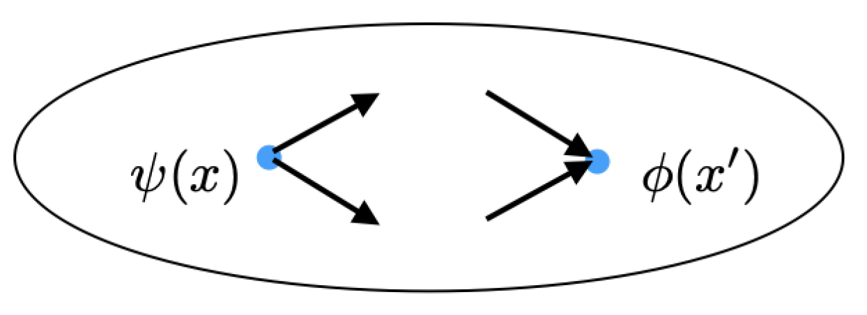
4.3. Two-Point Functions

Two-state formalisms are receiving much attention at present [39], but we will motivate our approach from within the Riemannian space formalism of relativity theory. In relativity, it is necessary to talk about events and not about point particles in motion. Events occur as a result of changes in energy momentum flows, and we propose taking the flow as our basic concept. The resulting flow lines can then be interpreted as “trajectories” in order to provide a simple but successful approximation to non-relativistic classical mechanics.

An event will have internal structure, but as a first approximation, it can be localized to a position on a suitable coordinate grid specified by four real parameters $x^{\mu }$. Notice that we are not localizing a point particle but a more nebulous structure, which we will describe with a field $\psi \left(\mathit{x}\right)$. Because we have no rigid extended structures in relativity, as we have in Euclidean space, we require two fields to define a neighborhood relation. This provides more evidence of the need to adopt $\rho (x,x^{\prime })$ as a primitive form to describe an unfolding process, as we will show. In fact, we require a new principle, which Eddington [40] expressed in the following form:

Everything connected with location, which enters into observational knowledge—everything we can know about the configuration of events—is contained in a relation of extension between pairs of events.

It is this relationship that Weyl [18] addressed with his gauge principle, forming a key part of our discussion.

We will follow Synge [17], who already revealed the need for a basic two-point characteristic function or “World Function” $\Omega (x,x^{\prime })$, which will provide a dynamic neighborhood relationship. Synge considered this function to be an extension of Hamilton’s principal or characteristic function that would encompass quantum phenomena. The traditional way of establishing neighborhood relations is through differentiation, but quantum mechanics distinguishes between “forward” derivatives and “backward” derivatives [41], with the wave function being subjected to the “forward” derivative while the “backward” derivative operates on the dual wave function. This distinction is essential for the Dirac particle, as has been clearly brought to light by Schwinger [36]. A detailed mathematical discussion of the “forward” and “backward” derivatives for the Dirac equation, where they are designated as $D_L$ and $D_R$, respectively, can be found in the work of Gilbert and Murray [42].

Synge [17] showed that all these subtleties lead to a two-point metric tensor $g_{\mu {\nu }^{\prime }}(x,x^{\prime })$. Notice the prime that is also on the $\nu$. It is in the coincident limit $x\to x^{\prime }$, where this two-point metric tensor becomes the usual metric tensor $g_{\mu \nu }\left(x\right)$. Thus, the traditional approach to the geometry of Riemannian spaces emerges as the coincidence limit when the two point events become fused into one. The relevance of this discussion to our algebraic approach to quantum phenomena already appeared in DeWitt’s paper [5], where we see that in the non-relativistic limit, the propagator becomes $\rho (x,x^{\prime })$, which was also used by Dirac [38]. Synge’s approach ties this propagator to the two-point metric tensor, which is a connection we exploit as we proceed.

But before continuing, we want to draw attention to the importance of coincident limits for quantum processes. This has been brought to light by Fröhlich [43] and one of us [44]. The Fröhlich paper is of particular importance, as he presented a detailed discussion of the emergence of the classical limit from the two-point function $\rho (x,x^{\prime })$. Crucially, he showed the necessity of using a two-point function when handling derivatives involving differences in position (i.e., derivatives of the form $\partial /\partial (x^{\prime }-x)$).

Indirectly related to this technical point, the limiting process is of fundamental significance in light of Gromov’s “non-squeezing theorem” [45,46]. This is a theorem in symplectic topology and has consequences for both classical mechanics and quantum mechanics. The fact that the theorem is relevant to classical mechanics shows that it is the harbinger of the Heisenberg uncertainty principle.

However, in this context, Gromov’s theorem has a dynamical origin and little to do with classical mechanics in a stochastic background field. Put simply, it “locks together” the two points in configuration space with two points in momentum space, ensuring $\Delta x\Delta p\ne 0$. In this sense, it introduces a semi-rigid element into relativistic physics. For a detailed discussion of this work, we refer to the work of de Gosson [8].

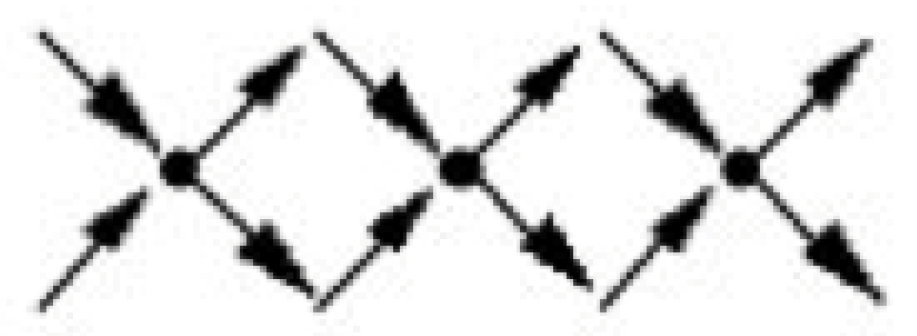
4.4. From de Broglie’s Double Solution to Bohm’s Structure Process

An essential feature of Bohm’s structure process is that motion is thought of as an event unfolding and then enfolding back into the background. The frequency of the process will be determined by the physics. As Penrose [47] reminds us, the mass of a particle provides a definite time measure along its world line through the Planck relation $m{c}^2=h\nu$. When applied to a stable particle, the mass $m_0$ determines a precise clock rate as given by the frequency $\nu$. Note also that $m_0/\nu =h/c^2$, which is a universal constant. The unfolding-enfolding rate is quite rapid, and thus the process can be approximated to a continuous energy flow as symbolized in Figure 2 and Figure 3.

Enfolding energy resonates with the Huygens construction which, as Feynman [48] remarked, provides a simple physical picture of the propagator. Bohm merely added an unfolding aspect to the process. Indeed, earlier Dirac [49] had written “The variation with time of the Heisenberg dynamical variables may thus be looked upon as the continuous unfolding of a unitary transformation”, which he summarized mathematically in his equation (Equation (60)) [49].

In this way, the continuous “trajectories” calculated by Philippidis, Dewdney and Hiley [13] appear as energy flow lines analogous to those shown in Berry [11,12] for optical flow lines. Furthermore, it can be shown that the quantum “trajectories” are an average of an ensemble of Feynman paths [50]. This then provides us with an intuitive image of the Heisenberg equation of motion (Equation (11)).

4.5. The Idempotent and Dirac’s Standard Bra–Ket

Let us now turn to see how these intuitive ideas can be used to develop a rigorous algebraic approach. Standard quantum mechanics focuses on irreducible representations, and to find these representations, we follow Weyl [51] and look for primitive idempotents. Unfortunately, the Heisenberg algebra is nilpotent and therefore has no idempotents. This is not a good start!

For a formal mathematical way of dealing with this problem, see the work of Schempp [52]. We will approach this problem in an informal way. In spite of the absence of an idempotent in the Heisenberg algebra, the success of Weyl’s use of primitive idempotents for the rotation group [51] prompted Dirac [53] to propose a generalization by singling out a distinguished ket and bra, with the standard ket $|S\rangle$ and the corresponding standard bra $\langle S|$, from which we can form an idempotent ${ϵ}_S=|S\rangle \langle S|$. Clearly, ${ϵ}_S^2={ϵ}_S$. Then, as Schönberg [54,55] showed in detail, we can add this element to the Heisenberg algebra to form an extended Heisenberg algebra [56].

Dirac fully developed the consequences of this additional element in his book Lectures on Quantum Mechanics and Relativistic Field Theory [57] while working within Hilbert space. However, we want to escape the limitations of the Hilbert space formalism. To achieve, this we must replace the standard wave function with an element of the minimal left ideal of the extended Heisenberg algebra ${\Psi }_L\left(x\right)={\psi }_L\left(x\right)ϵ\in {\mathcal{I}}_L\left(x\right)$, where ${\psi }_L\left(x\right)\in \mathbb{R}$. The dual wave function is replaced with an element of a minimal right ideal ${\Psi }_R\left(x\right)=ϵ{\psi }_R\left(x\right)\in {\mathcal{I}}_R\left(x\right)$.

Thus, if we now define $\rho (x,x^{\prime })={\psi }_L\left(x\right){ϵ}_x{\psi }_R\left(x^{\prime }\right)$, then in the coincident limit, we have $\rho (x,x^{\prime })\to {\rho }_c\left(x\right)$. In this way, we find ${\rho }_c\left(x\right)={\Psi }_L\left(x\right){\Psi }_R\left(x\right)$ which is, of course, the density matrix in the standard approach. The pure state is then simply characterized by ${\rho }_c{\left(x\right)}^2={\rho }_c\left(x\right)$. Once again, we see that the coincident limit agrees with the standard approach, and thus what have we achieved?

If we want phase information, then we must use the two-point function $\rho (x,x^{\prime })$. It is this generalized function that enables us to find the quantum potentials for the Pauli spin and Dirac relativistic equations [58].

Finally, note that the averages of the dynamical variables can then be found using $\langle A\rangle =tr\left(A{\rho }_c\right)$. This highlights the basic features of what we call the Algebraic Way [59]. It is through this method that we can explore the geometric content of quantum phenomena.

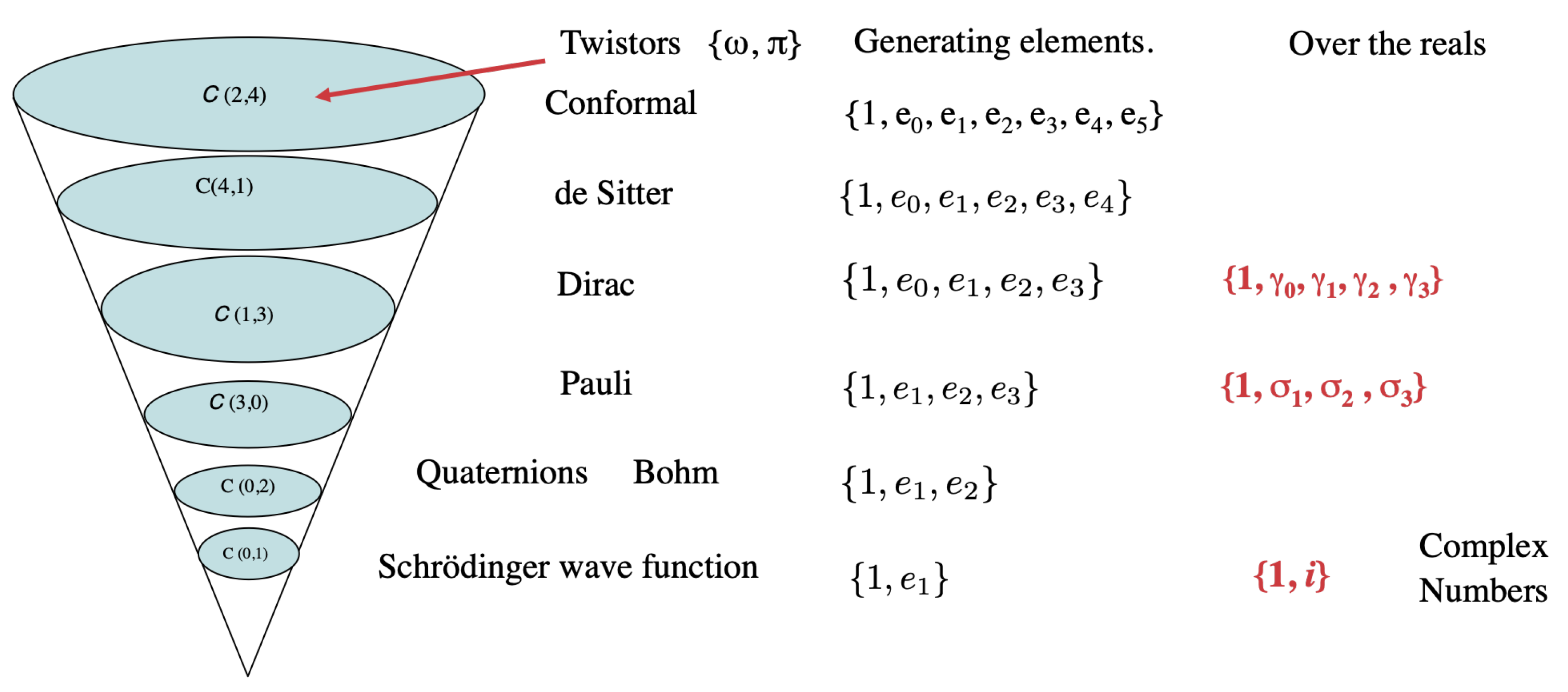
5. The Orthogonal Clifford Algebras

5.1. Which Non-Commuting Algebra?

Clearly, the Heisenberg algebra must play an important role, but for spin problems, it is the orthogonal group that is central. Historically, Clifford played a key part in the development of non-commuting orthogonal algebras. What was remarkable and of particular significance for the content of this paper was Clifford’s interest in what should underlie classical mechanics in very small, and this was before any notion of quantum mechanics had appeared in the literature. After discussing Riemann’s ideas, Clifford [60] wrote the following:

…although the axioms of solid geometry are true within the limits of experiment for finite portions of our space, yet we have no reason to conclude that they are true for very small portions; and if any help can be got thereby for the explanation of physical phenomena, we may have reason to conclude that they are not true for very small portions of space.

A quick way of illustrating the importance of the orthogonal Clifford algebras to modern physics is to consider Figure 4, where we see a tower of relationships of the algebras generated over the real field.

In the diagram, ${\mathit{e}}_i$ represents the generators of the algebra and $C(p,q)$ is the Clifford algebra with a $(p,q)$ metric of p positive squares and q negative squares. The Pauli spin matrices, the Dirac gamma matrices and the Penrose twistors are merely representations of the generators of their respective algebras.

Figure 4’s tower is formed using a simple generating relationship:

$$\begin{array}{c}\hfill C(p+1,q+1)=C(p,q)\oplus C(1,1).\end{array}$$

What makes this algebra easy to manipulate is that the whole tower closes on eight generators because of Bott periodicity [61].

5.2. The Role of the Clifford Algebra

We appear to have two seemingly very different algebras: the Heisenberg algebra with its symplectic symmetry and the Clifford algebra generated from the orthogonal group. A symplectic vector space involves the invariance of an antisymmetric form $F(x,y)$, whereas an orthogonal space is defined by the invariance of a symmetric quadratic form $g(x,y)$.

Nevertheless, there is a common group at the intersection of the symplectic and orthogonal groups, namely the unitary group. Furthermore, it is the unitary group that lies at the heart of quantum mechanics. The full mathematical structure of this space requires combining the orthogonal Clifford algebra with the symplectic Clifford algebra [62,63]. For the purposes of this paper, we need only be familiar with the much-used orthogonal Clifford algebra, leaving discussion of the symplectic group for a later paper.

We simply note here that we are replacing discrete events with more familiar continuous mathematics where differentiation will be available to us. This means that we must replace discrete simplicial structures like chains and cochains with differential fields and differential forms. The orthogonal Clifford algebra allows such a generalization (see Benn and Tucker [64] for details). A more radical approach can be found in the work of Hiley [65].

We now choose an appropriate Clifford algebra $\mathcal{A}$ with a suitable idempotent $ϵ$ and form an element of a minimal left ideal ${\mathcal{I}}_L={\psi }_Lϵ$, where

$$\begin{array}{c}\hfill {\psi }_L=a+\sum _j{a}_j{e}_j+\sum _{j>k}{a}_{jk}{e}_j{e}_k+\sum _{j>k>n}{a}_{jkn}{e}_j{e}_k{e}_n+\cdots =S+V+B+T\cdots \end{array}$$

Thus, the elements of the left ideal contain information about geometric entities such as scalars, vectors, bivectors and trivectors.

An important feature that a Clifford algebra brings with it is the Clifford group G. Let G be the set of invertible elements $g\in C\left(Q\right)$ such that

$$\begin{array}{c}\hfill {\varphi }_g\left(x\right)=gx{g}^{-1}\in E,\forall x\in E.\end{array}$$

If we choose the invertible element g to be a product of two elements $g=uv$, we find rotations are induced by twisted products defined by

$$\begin{array}{c}\hfill x\to uvx{v}^{-1}{u}^{-1}.\end{array}$$

We can understand this process by recalling that a rotation may be formed using a pair of reflections u and v.

Since all the information contained in the wave function is encoded in the elements of a minimal left ideal, we see that this information is deeply related to geometric structures in the spacetime geometry. We should therefore not be surprised to find dynamical information appearing in the amplitude of the wave function.

5.3. The Algebraic Schrödinger Particle

The algebra that forms the basis of the Schrödinger equation emerges from the quaternion Clifford algebra $C(0,2)$ taken over the real field [23]. A general expression for an element of a left ideal can be written as

$$\begin{array}{c}\hfill {\psi }_L=g_0+g_1{e}_1+g_2{e}_2+g_3{e}_1{e}_2.\end{array}$$

If we now choose the pair of elements $(g_0+g_1{e}_1)$ and write $e_1=i$, then we can identify $(g_0,g_1)$ with the pair $({\psi }^{*},\psi )$ through the relation

$$\begin{array}{c}\hfill g_0=({\psi }^{*}+\psi )/2;g_1=i({\psi }^{*}-\psi )/2\mathrm{where}{g}_0,g_1\in \mathbb{R}.\end{array}$$

It should be noticed that in identifying $e_1$ with i, we have simply made contact with the conventional approach so that now $\psi$ can be used as part of the quantum algorithm, as Bohr [66] called it. We insist that our mathematical structure must retain the algebraic meaning of $e_1$. The element of the left ideal is in the algebra so that the element $(g_0+g_1{e}_1)$ is in the algebra and therefore describes an unfolding process.

5.4. The Pauli Particle

As we can see in Figure 4, the Pauli particle is described by the elements of the Clifford algebra $C(3,0)$. Traditionally, we define the z axis by means of a homogeneous magnetic field. In the algebra, this is accomplished by choosing the idempotent ${ϵ}_P=(1+{\sigma }_3)/2$, where ${\sigma }_3$ is the diagonal Pauli spin matrix. With this idempotent, a general element of a minimal left ideal can be written in the form

$$\begin{array}{c}\hfill {\psi }_L=g_0+g_1{\sigma }_{23}+g_2{\sigma }_{13}+g_3{\sigma }_{12}.\end{array}$$

Here, ${\sigma }_{ij}={\sigma }_i{\sigma }_j$ is a product of two Pauli spin matrices, which is a geometric bivector. Although it still behaves like a quaternion, it is now represented by a $2\times 2$ matrix, adding new structure. In the Schrödinger case, $e_i$ represents vectors, a rather different geometric object.

For comparison with the standard form of the Pauli spinor

$$\begin{array}{c}\hfill \Psi =\left(\begin{array}{c}{\psi }_1\\ {\psi }_2\end{array}\right)=\left(\begin{array}{c}{R}_1{e}^{i{S}_1}\\ R_2{e}^{i{S}_2}\end{array}\right)\end{array}$$

we identify

$$\begin{array}{c}\hfill g_0=({\psi }_1^{*}+{\psi }_1)/2;g_1=i({\psi }_2^{*}-{\psi }_2)/2;g_2=({\psi }_2^{*}+{\psi }_2)/2;g_3=i({\psi }_1^{*}-{\psi }_1)/2\end{array}$$

where $g_0,g_1,g_2$ and $g_3$ are in $\mathbb{R}$.

5.5. The Dirac Particle

In this case, the primitive idempotent is ${ϵ}_D$, and we have chosen to make a comparison with the Dirac spinor in the standard form

$$\begin{array}{c}\hfill \Psi =\left(\begin{array}{c}{\psi }_1\\ {\psi }_2\\ {\psi }_3\\ {\psi }_4\end{array}\right)=\left(\begin{array}{c}{R}_1{e}^{i{S}_1}\\ R_2{e}^{i{S}_2}\\ R_3{e}^{i{S}_3}\\ R_4{e}^{i{S}_4}\end{array}\right).\end{array}$$

Using ${ϵ}_D=(1+{\gamma }_0)(1+i{\gamma }_{12})/4$, we find

$$\begin{array}{c}\hfill {\psi }_L=a+b{\gamma }_{12}+c{\gamma }_{23}+d{\gamma }_{13}+f{\gamma }_{01}+g{\gamma }_{02}+h{\gamma }_{03}+n{\gamma }_5\end{array}$$

with $a,b,c,d,f,g,h,n\in \mathbb{R}$. Here, ${\gamma }_{ij}={\gamma }_i{\gamma }_j$ are products of the Dirac $\gamma$ matrices identified with the generators of the Clifford algebra $C(1,3)$.

Thus, we see that for all species of “particle”, information regarding the properties of the “particle” is contained in the algebra itself in the elements of the appropriate minimal left ideals. Therefore, when working with the non-commutative Clifford algebra, there is no need for a Hilbert space, as all the relevant information about the “particle” is in the algebra already. Since the algebra is about a “process”, which we have called “flow” in this paper, there is no collapse of anything. There is simply a flow of energy, an energy that nevertheless has quantum properties.

The full working details of the approach can be found in the following papers [58,67,68,69]. Here, we will simply give the general equations describing the quantum flow. Note that these two equations work for all types of particle, replacing the individual wave equations used in the standard approach. The first dynamical equation reads

$$\begin{array}{c}\hfill i{\partial }_t{\rho }_c=\left(\overrightarrow{H}{\Phi }_L\right){\tilde{\Phi }}_L-{\Phi }_L\left({\tilde{\Phi }}_L\overleftarrow{H}\right):={[H,{\rho }_c]}_{-}.\end{array}$$

This equation describes the continuity equation for mass-density flow. The conservation of energy in the flow is described by the equation

$$\begin{array}{c}\hfill {\Phi }_L\overleftrightarrow{{\partial }_t}{\tilde{\Phi }}_L=\left(\overrightarrow{H}{\Phi }_L\right){\tilde{\Phi }}_L+{\Phi }_L\left({\tilde{\Phi }}_L\overleftarrow{H}\right):={[H,{\rho }_c]}_{+}.\end{array}$$

Using these equations, we find a hierarchy of “quantum” potentials. The potential for the free Dirac particle is

$$\begin{array}{c}\hfill Q_D={\Pi }^2+W^2+[J{\partial }_{\mu }{W}^{\mu }+{\partial }_{\mu }{W}^{\mu }J].\end{array}$$

The potential for the Pauli particle is

$$\begin{array}{c}\hfill Q_P=W_P^2/2m+[S(\nabla W_P)+(\nabla W_P)S]/m.\end{array}$$

(12)

Meanwhile, the potential for the Schrödinger particle is

$$\begin{array}{c}\hfill Q_S=-\frac{{\hslash }^2}{2m}\frac{{\nabla }^2\sqrt{\rho }}{\sqrt{\rho }}.\end{array}$$

Note that extra terms arise as we add spin and relativity to the structure of the flow. A beautiful illustration of the contribution of the spin in the case of the Pauli flow can be found in the works of Dewdney, Holland, Kyprianidis and Vigier [70]. They used an earlier method based on Euler angles which produces the same results as the expression in Equation (12).

6. Compensating Fields in Quantum Mechanics

Having seen that it is possible to generalize the quantum potential to include spin and relativity, we return to considering in more detail how the metric tensor gives rise to electric- and magnetic-type fields for charge-density flows which can immediately be generalized to mass-density flows, a highly relevant step for the topics discussed in this paper.

6.1. Weak Static Fields: The First Approximation

Consider two particles evolving in their mutual gravitational field $\varphi$. In Riemannian spacetime, the first approximation to the metric tensor is to choose $g_{00}=(1+2\varphi /c^2);g_{0j}=g_{j0}=0$ and $g_{ij}\ne 0$ so that the metric becomes

$$\begin{array}{c}\hfill d{s}^2=(1+2\varphi /c^2)c^{2}d{t}^2-d{l}^2\end{array}$$

where $d{l}^2$ is the usual Euclidean 3-metric [20].

To find the mass-density flow geodesic described by this metric, we have to find the stationary value of $\int ds$ where

$$\begin{array}{c}\hfill {\int }_{P_1}^{P_2}ds=c{\int }_{t_1}^{t_2}\left(1+\frac{\varphi }{c^2}-\frac{v^2}{2c^2}\right)dt=c(t_2-t_1)-\frac{1}{c}{\int }_{t_1}^{t_2}\left(\frac{v^2}{2}-\varphi \right)dt.\end{array}$$

Notice that obtaining the stationary value of $\int ds$ is equivalent to finding the stationary value of

$$\begin{array}{c}\hfill \int \left(\frac{v^2}{2}-\varphi \right)dt\end{array}$$

which is just Hamilton’s principle for a particle moving in a gravitational potential $\varphi$. Here, the force acting on this flow depends only on the position.

6.2. Weak Field: The Second Approximation

Let us continue to the next approximation by removing the restriction $g_{j0}=0$. This enables us to construct terms involving the velocities $d{x}^i/dt$, which will lead to the appearance of a velocity-dependent force. To meet this aim, we follow the work of Rindler [20] and introduce a mass-density vector potential $\mathcal{A}$ by simply writing $A_{i}d{x}^i/dt=\mathcal{A}.\mathit{v}$. We then have

$$\begin{array}{c}\hfill d{s}^2=(1+2\varphi /c^2)\left(1-\frac{2\mathcal{A}.\mathit{v}}{c^3}\right)c^{2}d{t}^2-d{l}^2\approx \left(1+\frac{2\varphi }{c^2}-\frac{2\mathcal{A}.\mathit{v}}{c^3}\right)c^{2}d{t}^2-d{l}^2\end{array}$$

which gives

$$\begin{array}{c}\hfill {\int }_{P_1}^{P_2}ds=c(t_2-t_1)-\frac{1}{c}{\int }_{t_1}^{t_2}\left(\frac{v^2}{2}-\varphi +\frac{\mathcal{A}.\mathit{v}}{c}\right)dt.\end{array}$$

Now, we have a net force acting on the particle which depends on the position and velocity since

$$\begin{array}{c}\hfill \mathit{f}=-\nabla \varphi +\mathit{v}\times (\nabla \times \mathcal{A})/c.\end{array}$$

Thus, we have constructed a gravitational analogue of the electromagnetic Lorentz force expressed in terms of a mass-density four-potential $(\varphi ,\mathcal{A})$. No mass charge appears because of the principle of equivalence. Note that the Coriolis force arises directly from the term featuring the angular velocity $\nabla \times \mathcal{A}/2c$ [20]. We should stress here that we have only considered a second-order approximation. Higher-order terms that destroy linearity have been neglected. These terms will be considered in a later paper.

6.3. The Role of the Energy–Momentum Tensor

To construct the energy–momentum tensor of the mass-density flow, we will follow de Broglie [3] and Takabayasi [71] and generalize the usual relativistic particle Lagrangian by allowing for a variable rest mass $M_0(\mathit{x},t)$. The rest mass changes when the energy flow undergoes acceleration. In this case, the Lagrangian of free mass-density flow takes the form

$$\begin{array}{c}\hfill \mathcal{L}=-M_0{c}^2{\left(1-\frac{v^2}{c^2}\right)}^{1/2}.\end{array}$$

Then, Hamilton’s principle of stationary action produces a generalized Hamilton–Jacobi equation with the relativistic Hamiltonian

$$\begin{array}{c}\hfill H=M_0{c}^2{\left(1-\frac{v^2}{c^2}\right)}^{-1/2}.\end{array}$$

The kinetic energy emerging from this Hamiltonian is simply $M_0{v}^2/2$. Both Lanczos [72] and Takabayasi [71] showed how an extra scalar field can be envisaged as a change in rest energy. Takabayasi wrote

$$\begin{array}{c}\hfill M_0{c}^2=m_0{c}^2+fU\end{array}$$

(13)

where $fU$ is the extra scalar field. Thus a rest mass shift $\delta m=fU/c^2$ occurs so that the kinetic energy becomes

$$\begin{array}{c}\hfill \mathrm{K}.\mathrm{E}.=\frac{1}{2}{v}^2\left(m_0+\frac{fU}{c^2}\right).\end{array}$$

If we write $fU=-{\lambda }^2{\nabla }^{2}A/2m_{0}A$, then we see the correction to the quantum Hamiltonian that DeWitt referred to when considering the principle of general covariance. This correction can be seen to have its origins in the change in the rest mass-density. Replacing $\lambda$ with ℏ enables us to distinguish specifically quantum processes.

This process has a consequence for Feynman’s path integrals. It should be recalled that Feynman [48] found it necessary to introduce a change in mass $m(1+\delta )$ “for a short time, $\delta ϵ$” in order to avoid the appearance of infinities in the limit $\delta ϵ\to 0$. Thus, we must introduce a change in the action of $(m/2){[(x_{k+1}-x_k)/ϵ]}^2\delta ϵ$. The usual expression for the kinetic energy diverges in the limit $ϵ\to 0$. As a consequence, the kinetic energy must be written in the form

$$\begin{array}{c}\hfill \mathrm{K}.\mathrm{E}.=\frac{1}{2}m{[(x_{k+1}-x_k)/ϵ]}^2+\hslash /2ϵi\end{array}$$

which is equivalent to writing it in the form

$$\begin{array}{c}\hfill \mathrm{K}.\mathrm{E}.=\frac{1}{2}m\left(\frac{x_{k+1}-x_k}{ϵ}\right)\left(\frac{x_k-x_{k-1}}{ϵ}\right).\end{array}$$

Feynman showed this expression to be finite in the limit $ϵ\to 0$. Therefore, writing the rest energy in the form of Equation (13) not only covers the Feynman case but is more general, arising whenever the mass-flow involves acceleration from whatever cause. We therefore have the emergence of the extra energy term ${\hslash }^2\mathcal{Q}$, which DeWitt [5] showed must be added to the classical Hamiltonian to obtain a general covariant quantum Hamiltonian. Hence, the quantum potential energy is a necessary part of the covariant formalism and not ad hoc as originally claimed by Heisenberg [14].

6.4. Quantum Mechanics Revisited

We have now seen why an extra quality of energy, which Bohm [4] and DeWitt [5] called the quantum potential energy, appears in different guises in various quantum processes. de Broglie saw it appearing in an expression of the inertial mass where the rest mass appears to be modified. For Bohm, it arises in the polar decomposition of the wave function in the Schrödinger picture. DeWitt sees it appearing when quantum processes are described in pseudo-Riemannian space. For Feynman, it is a necessary addition to his path integral formalism in order to avoid singularities. Berry sees it arising in an expression of the curvature of the momentum streamlines in classical wave optics. In this paper, we have seen how the quantum potential arises naturally from an algebraic approach which replaces the wave function with an element of the left ideal from the algebra itself. This emphasizes the role of the individual dynamical process rather than having to rely only on the statistical features of an ensemble of individual processes.

6.5. Quantum Ambiguity

The reason for the appearance of the compensating field that we have been referring to in this paper can be traced back to the ambiguity highlighted in the Stone–von Neumann theorem. This theorem claims [32,33] that the Schrödinger representation is unique but only up to a unitary transformation, and these last few words are of vital importance. We have already seen that an ambiguity arises in defining covariant derivatives in the sense that covariant derivatives of general tensors are coordinate-dependent. For quantum processes, this ambiguity is highly significant because the second-order derivative ${\nabla }^{\mu }{\nabla }_{\mu }$ that is central to the quantum kinetic energy is not coordinate-independent. Thus, this coordinate ambiguity of differential geometry is carried over to the quantum formalism and is the source of the quantum potential energy.

We can remove this ambiguity by exploiting the unitary gauge ambiguity that arises from the Stone–von Neumann theorem. Indeed, we saw in Section 3 that conformal rescaling removes the ambiguity that arises in Riemannian geometry. From the quantum side, it is the gauge freedom that allows the various “pictures” to emerge, with the Schrödinger picture, the Heisenberg picture and the interaction picture being used the most [73]. We have found it particularly useful to introduce another little-known picture: the Dirac-Bohm picture [74].

As we have seen, the notion of a “quantum potential” first emerged from Bohm’s use of polar decomposition of the wave function in the non-relativistic Schrödinger picture. Here, it appears as if the amplitude of the wave function is acting as a source of energy over and above the kinetic energy, a strange and unexpected result. In the approach of DeWitt, the quantum potential appears in the Heisenberg picture as an additional term that must be added to the Hamiltonian as shown in Equation (1). This confirms that the quantum potential is an essential part of the dynamical geometry.

The Dirac–Bohm picture recently proposed by Hiley, Dennis and de Gosson [74] sees the role of the amplitude emerging in a rather simple way. In this picture, a conformal rescaling $g^{jk}={\Omega }^2{\overline{g}}^{jk}$ must be compensated by the change $\psi =\Omega \overline{\psi }$. This means

$$\begin{array}{c}\hfill \psi =A{e}^{iS/\hslash }=\Omega \overline{\psi }=\Omega e^{iS/\hslash }\mathrm{so}\mathrm{that}A=\Omega .\end{array}$$

Let us put $A=\Omega$ into the expression for the Ricci scalar curvature given in Equation (8), and we find

$$\begin{array}{c}\hfill \overline{\mathcal{R}}=-6{\Omega }^{-2}\left[\frac{\square \Omega }{\Omega }\right]=-6{\Omega }^{-2}\left[\frac{\square A}{A}\right]\end{array}$$

which agrees with Delphenich [75]. A similar result was found by Santamato [76], who claimed that this sort of feedback between geometry and dynamics is proven to be the origin of quantum effects. The relativistic quantum potential (omitting ${\hslash }^2/2m_0$ here in order to focus on the curvature) is $Q=\square A/A$ so that

$$\begin{array}{c}\hfill Q=-\overline{\mathcal{R}}{\Omega }^2/6=-\rho \overline{\mathcal{R}}/6\mathrm{where}\rho =A^2.\end{array}$$

In this way, we see how the dynamics is encoded in the wave function through the amplitude. Moreover, we have shown how the information that is encoded in the wave function is encoded in the dynamical algebra itself: through elements of a minimal left ideal. Thus, rather than being surprised at seeing the amplitude containing dynamical information, we should expect it. The dynamics expressed through the differential geometry is encoded in the quantum algorithm.

This confirms the view developed in this paper, namely that the dynamics of the individual quantum process is contained in the non-commutative algebra itself. Hilbert space is not necessary. The wave function formalism should be regarded as an algorithm in exactly the same way that Bohr [66] pointed out. Therefore, while we fully support this particular feature of Bohr’s view, we have shown how it is possible to obtain a deeper understanding of quantum phenomena in terms of individual processes, something Bohr tried to rule out using his principle of complementarity. Our approach circumnavigates this philosophical obstruction by abandoning the traditional assumption that physics involves “particles evolving in an a priori given space-time manifold”. Instead, our approach takes the process as being basic and identifies the particles with invariant features of the energy-density or mass-density flow from which, ultimately, the spacetime manifold itself emerges.

References

1. de Broglie, L. La mécanique ondulatoire et la structure atomique de la matière et du rayonnement. J. de Physique et Le Radium 1927, VIII, 225–241. [Google Scholar] [CrossRef]
2. de Broglie, L.; Brillouin, L. Selected Papers on Wave Mechanics; Blackie and Son: London, UK, 1928; pp. 113–138. [Google Scholar]
3. de Broglie, L. Non-Linear Wave Mechanics: A Causal Interpretation; Elsevier: Amsterdam, The Netherlands, 1960; pp. 217–218. [Google Scholar]
4. Bohm, D. A Suggested Interpretation of the Quantum Theory in Terms of Hidden Variables, I. Phys. Rev. 1952, 85, 166–179. [Google Scholar] [CrossRef]
5. DeWitt, B.S. Point Transformations in Quantum Mechanics. Phys. Rev. 1952, 85, 653–661. [Google Scholar] [CrossRef]
6. Penrose, R.; Rindler, W. Spinors and Space-Time; Cambridge University Press: Cambridge, UK, 1984; Volume 1. [Google Scholar]
7. de Broglie, L. The Reinterpretation of Wave Mechanics. Found. Phys. 1970, 1, 5–15. [Google Scholar] [CrossRef]
8. de Gosson, M.A. The Principles of Newtonian and Quantum Mechanics: The Need for Planck’s Constant; Imperial College Press: London, UK, 2017. [Google Scholar]
9. DeWitt, B. Dynamical Theory in Curved Spaces, I. A review of the Classical and Quantum Action Principles. Rev. Mod. Phys. 1957, 29, 377–397. [Google Scholar] [CrossRef]
10. Schulman, L.S. Techniques and Applications of Path Integration; Dover: New York, NY, USA, 2005; p. 216. [Google Scholar]
11. Berry, M.V. Curvature of wave streamlines. J. Phys. A Math. Theor. 2013, 46, 395202. [Google Scholar] [CrossRef]
12. Berry, M.V. Optical Currents. J. Opt. A Pure Appl. Opt. 2009, 11, 094001. [Google Scholar] [CrossRef]
13. Philippidis, C.; Dewdney, D.; Hiley, B.J. Quantum Interference and the Quantum Potential. Il Nuovo Cimento 1979, 52B, 15–28. [Google Scholar] [CrossRef]
14. Heisenberg, W. Physics and Philosophy: The Revolution in Modern Science; George Allen and Unwin: London, UK, 1958. [Google Scholar]
15. Nelson, E. Derivation of Schrödinger’s Equation from Newtonian Mechanics. Phys. Rev. 1966, 150, 1079–1085. [Google Scholar] [CrossRef]
16. Bliokh, K.Y.; Bekshaev, A.Y.; Kofman, A.G.; Nori, F. Photon trajectories, anomalous velocities and weak measurements: A classical interpretation. New J. Phys. 2013, 15, 073022. [Google Scholar] [CrossRef]
17. Synge, J.L. Relativity: The General Theory; North-Holland: Amsterdam, The Netherlands, 1964. [Google Scholar]
18. Weyl, H. Space, Time, Matter; Dover: London, UK, 1922. [Google Scholar]
19. Borges, E.; Braga, J.P. O efeito de Coriolis: De pêndulos a moléculas. Quim. Nova 2010, 33, 1416–1420. [Google Scholar] [CrossRef]
20. Rindler, W. Relativity: Special, General, and Cosmological; Oxford University Press: Oxford, UK, 2006. [Google Scholar]
21. Penrose, R. Conformal Treatment of Infinity. In Relativity, Groups and Topology; DeWitt, C., DeWitt, B., Eds.; Les Houches Summer School of Theoretical Physics, Grenoble; Blackie and Son: London, UK, 1963; pp. 567–584. [Google Scholar]
22. Wald, R.M. General Relativity; University of Chicago Press: Chicago, IL, USA, 1984. [Google Scholar]
23. Dyson, F.J. The Threefold Way. Algebraic Structure of Symmetry Groups and Ensembles in Quantum Mechanics. J. Math. Phys. 1962, 3, 1199–1215. [Google Scholar] [CrossRef]
24. Penrose, R. On Gravity’s Role in Quantum State Reduction. Gen. Relativ. Gravit. 1996, 28, 581–600. [Google Scholar] [CrossRef]
25. Schouten, J.A. Dirac Equations in General Relativity (Four-dimensional Theory). J. Math. Phys. 1931, X, 239–271. [Google Scholar] [CrossRef]
26. Clifford, W.K. Preliminary Sketch of Biquaternions. Proc. Lond. Math. Soc. 1873, IV, 381–395. [Google Scholar] [CrossRef]
27. Clifford, W.K. The Common Sense of the Exact Sciences; Kegan Paul, Trench & Co.: London, UK, 1886. [Google Scholar]
28. Penrose, R. Twistor Algebra. J. Math. Phys. 1967, 8, 345–366. [Google Scholar] [CrossRef]
29. Penrose, R.; Rindler, W. Spinors and Space-Time; Cambridge University Press: Cambridge, UK, 1986; Volume 2. [Google Scholar]
30. Haag, R. Local Quantum Physics; Springer: Berlin, Germany, 1992. [Google Scholar]
31. Emch, G.G. Algebraic Methods in Statistical Mechanics and Quantum Field Theory; Wiley-Interscience: New York, NY, USA, 1972. [Google Scholar]
32. von Neumann, J. Letter to G. Birkhoff, 1935 as reported in Birkoff, G., Lattice Theory. In American Mathematical Society Colloqium Publications; American Mathematical Society: Providence, RI, USA, 1966; p. 25. [Google Scholar]
33. Rédei, M. Why von Neumann did not like the Hilbert space formalism of quantum mechanics (and what he liked instead). Stud. Hist. Philos. Mod. Phys. 1996, 27, 493–510. [Google Scholar] [CrossRef]
34. Bohm, D. Space, Time, and the Quantum Theory Understood in Terms of Discrete Structural Process. In Proceedings of the International Conference on Elementary Particles, Kyoto, Japan, 24–30 September 1965; pp. 252–287. [Google Scholar]
35. Dirac, P.A.M. On the Analogy Between Classical and Quantum Mechanics. Rev. Mod. Phys. 1945, 17, 195–199. [Google Scholar] [CrossRef]
36. Schwinger, J. On Gauge Invariance and Vacuum Polarization. Phys. Rev. 1951, 82, 664–679. [Google Scholar] [CrossRef]
37. Bohm, D. Wholeness and the Implicate Order; Appendix of Chapter 6; Routledge: London, UK, 1980. [Google Scholar]
38. Dirac, P.A.M. On the Annihilation of Electrons and Protons. Math. Proc. Camb. Philos. Soc. 1930, 26, 361–375. [Google Scholar] [CrossRef]
39. Aharonov, Y.; Vaidman, L. The Two-State Vector Formalism: An Updated Review. Lect. Notes Phys. 2008, 73, 399–447. [Google Scholar]
40. Eddington, A.S. The Mathematical Theory of Relativity; Cambridge University Press: Cambridge, UK, 1937; p. 10. [Google Scholar]
41. Hiley, B.J. Structure Process, Weak Values and Local Momentum. J. Phys. Conf. Ser. 2016, 701, 012010. [Google Scholar] [CrossRef]
42. Gilbert, J.; Murray, M. Clifford Algebras and Dirac Operators in Harmonic Analysis; Cambridge Studies in Advanced Mathematics; Cambridge University Press: Cambridge, UK, 1991. [Google Scholar]
43. Fröhlich, H. Microscopic Derivation of the Equations of Hydrodynamics. Physica 1967, 37, 215–226. [Google Scholar] [CrossRef]
44. Hiley, B.J. Non-commutative Quantum Geometry: A re-appraisal of the Bohm approach to quantum theory. In Quo Vadis Quantum Mechanics? Elitzur, A., Dolev, S., Kolenda, N., Eds.; Springer: Berlin, Germany, 2005; pp. 299–324. [Google Scholar]
45. Gromov, M. Pseudo holomorphic curves in symplectic manifolds. Invent. Math. 1985, 82, 307–347. [Google Scholar] [CrossRef]
46. de Gosson, M.A. The symplectic egg in classical and quantum mechanics. Am. J. Phys. 2013, 81, 328–337. [Google Scholar] [CrossRef]
47. Penrose, R. Fashion, Faith and Fantasy in the New Physics of the Universe; Princeton University Press: Princeton, NJ, USA, 2016; p. 55. [Google Scholar]
48. Feynman, R.P. Space-time Approach to Non-Relativistic Quantum Mechanics. Rev. Mod. Phys. 1948, 20, 367–387. [Google Scholar] [CrossRef]
49. Dirac, P.A.M. The Principles of Quantum Mechanics; Oxford University Press: Oxford, UK, 1947; p. 125. [Google Scholar]
50. Flack, R.; Hiley, B.J. Feynman Paths and Weak Values. Entropy 2018, 20, 367. [Google Scholar] [CrossRef]
51. Weyl, H. The Theory of Groups and Quantum Mechanics; Dover: London, UK, 1931. [Google Scholar]
52. Schempp, W. Harmonic Analysis on the Heisenberg Nilpotent Lie Group, with Applications to Signal Theory; Longman Scientific & Technical: London, UK, 1986. [Google Scholar]
53. Dirac, P.A.M. A new notation for quantum mechanics. Math. Proc. Camb. Philos. Soc. 1939, 35, 416–418. [Google Scholar] [CrossRef]
54. Schönberg, M. Quantum Mechanics and Geometry. An. Acad. Brasil. Cien. 1957, 29, 473–485. [Google Scholar]
55. Schönberg, M. Quantum Kinematics and Geometry. Nuovo Cimento Suppl. 1957, VI, 356–380. [Google Scholar] [CrossRef]
56. Hiley, B.J. Algebraic Quantum Mechanics, Algebraic Spinors and Hilbert Space. In Boundaries, Scientific Aspects of ANPA 24; Bowden, K.G., Ed.; ANPA Publications: London, UK, 2003; pp. 149–186. [Google Scholar]
57. Dirac, P.A.M. Lectures on Quantum Mechanics and Relativistic Field Theory; Notes by Gupta, K.K. and Sudershan, G.; Martino Publishing: Mansfield Centre, CT, USA, 2012. [Google Scholar]
58. Hiley, B.J.; Callaghan, R.E. Clifford Algebras and the Dirac-Bohm Quantum Hamilton-Jacobi Equation. Found. Phys. 2012, 42, 192–208. [Google Scholar] [CrossRef]
59. Hiley, B.J. The Algebraic Way, in Beyond Peaceful Coexistence, The Emergence of Space, Time and Quantum; Licata, I., Ed.; World Scientific: Singapore, 2016; pp. 1–25. [Google Scholar]
60. Clifford, W.K. On the Space-Theory of Matter. Proc. Camb. Philos. Soc. 1876, 2, 157–158. [Google Scholar]
61. Bott, R.; Mather, J. Topics in Topology and Differential Geometry. In Battelle Rencontres; DeWitt, C.M., Wheeler, J.A., Eds.; Benjamin: New York, NY, USA, 1968; pp. 460–515. [Google Scholar]
62. Crumeyrolle, A. Structures symplectiques, structures complexes, spineurs symplectiques et transformation de Fourier. J. Geom. Phys. 1985, 2, 107–134. [Google Scholar] [CrossRef]
63. Binz, E.; de Gosson, M.A.; Hiley, B.J. Clifford Algebras in Symplectic Geometry and Quantum Mechanics. Found. Phys. 2013, 43, 424–439. [Google Scholar] [CrossRef]
64. Benn, I.M.; Tucker, R.W. An Introduction to Spinors and Geometry with Applications in Physics; Adam Hilger: Bristol, UK, 1987. [Google Scholar]
65. Hiley, B.J. Process, Distinction, Groupoids and Clifford Algebras: An Alternative View of the Quantum Formalism. Lect. Notes Phys. 2011, 813, 705–750. [Google Scholar]
66. Bohr, N. Atomic Physics and Human Knowledge; Science Editions: New York, NY, USA, 1961. [Google Scholar]
67. Hiley, B.J.; Callaghan, R.E. The Clifford Algebra Approach to Quantum Mechanics A: The Schrödinger and Pauli Particles. arXiv 2010, arXiv:1011.4031. [Google Scholar]
68. Hiley, B.J.; Callaghan, R.E. The Clifford Algebra Approach to Quantum Mechanics B: The Dirac Particle. arXiv 2010, arXiv:1011.4033. [Google Scholar]
69. Hiley, B.J.; Van Reeth, P. Quantum Trajectories: Real or Surreal? Entropy 2018, 20, 353. [Google Scholar] [CrossRef]
70. Dewdney, C.; Holland, P.R.; Kyprianidis, A.; Vigier, J.-P. Spin and non-locality in quantum mechanics. Nature 1988, 336, 536–544. [Google Scholar] [CrossRef]
71. Takabayasi, T. Remarks on the Formulation of Quantum Mechanics with Classical Pictures and on Relations between Linear Scalar Fields and Hydrodynamical Fields. Prog. Theor. Phys. 1953, 9, 187–222. [Google Scholar] [CrossRef]
72. Lanczos, C. The Variational Principles of Mechanics; Dover: New York, NY, USA, 1970. [Google Scholar]
73. Schweber, S.S. Introduction to Relativistic Quantum Field Theory; Harper & Row: New York, NY, USA, 1961. [Google Scholar]
74. Hiley, B.J.; Dennis, G.; de Gosson, M.A. The Role of Geometric and Dynamical Phases in the Dirac-Bohm Picture. Ann. Phys. 2022, 438, 168759. [Google Scholar] [CrossRef]
75. Delphenich, D.H. The Geometric Origin of the Madelung Potential. arXiv 2002, arXiv:gr-qc/0211065. [Google Scholar]
76. Santamato, E. Geometric derivation of the Schrödinger equation from classical mechanics in curved Weyl spaces. Phys. Rev. D 1984, 29, 216–222. [Google Scholar] [CrossRef]
Figure 1. Streamlines emanating from two coherent optical sources [12].
Symmetry 16 00067 g001
Figure 2. A primitive image of the unfolding and enfolding of an event.
Symmetry 16 00067 g002
Figure 3. The continuous enfolding and unfolding of events.
Symmetry 16 00067 g003
Figure 4. Tower of Clifford algebras.
Symmetry 16 00067 g004
Disclaimer/Publisher’s Note: The statements, opinions and data contained in all publications are solely those of the individual author(s) and contributor(s) and not of MDPI and/or the editor(s). MDPI and/or the editor(s) disclaim responsibility for any injury to people or property resulting from any ideas, methods, instructions or products referred to in the content.