Article

Bifurcations Associated with Three-Phase Polynomial Dynamical Systems and Complete Description of Symmetry Relations Using Discriminant Criterion

by
Yury Shestopalov
1,*,
Azizaga Shakhverdiev
2 and
Sergey V. Arefiev
3
1
Department of Applied Mathematics, Russian Technological University MIREA, 119454 Moscow, Russia
2
Department of the Development and Operation of Oil and Gas Fields, Russian State Geological Prospecting University, 117485 Moscow, Russia
3
Department for the Development of Oil and Gas Fields in Western Siberia and the Perm Region, PJSC “LUKOIL”, 101000 Moscow, Russia
*
Author to whom correspondence should be addressed.
Symmetry 2024, 16(1), 14; https://doi.org/10.3390/sym16010014
Submission received: 25 October 2023 / Revised: 7 December 2023 / Accepted: 12 December 2023 / Published: 21 December 2023
(This article belongs to the Special Issue Three-Dimensional Dynamical Systems and Symmetry)

Abstract

:
The behavior and bifurcations of solutions to three-dimensional (three-phase) quadratic polynomial dynamical systems (DSs) are considered. The integrability in elementary functions is proved for a class of autonomous polynomial DSs. The occurrence of bifurcations of the type-twisted fold is discovered on the basis and within the frames of the elements of the developed DS qualitative theory. The discriminant criterion applied originally to two-phase quadratic polynomial DSs is extended to three-phase DSs investigated in terms of their coefficient matrices. Specific classes of D- and S-vectors are introduced and a complete description of the symmetry relations inherent to the DS coefficient matrices is performed using the discriminant criterion.

1. Introduction

Analysis of bifurcations in polynomial dynamical systems (DSs) constitutes a classical problem of the qualitative theory of DSs and differential equations and catastrophe theory and has been a subject of intense studies [1,2,3,4,5]. The main attention has been paid to non-autonomous polynomial DSs where many characteristic bifurcation types have been identified, including equilibriums, sinks, saddles, limit cycles. Autonomous polynomial DSs investigated in these studies, especially the case of two dimensions, are non-integrable and characterized by ‘mixed’ right-hand sides involving second-order polynomials in two variables.
We identify and consider an integrable family of three-dimensional (three-phase) polynomial quadratic DSs. We show, as an extension of a similar study performed in [6] for two-dimensional polynomial quadratic DSs, that one can carry out a complete investigation of singularities, and in this manner, create a complete qualitative theory in the three-phase case as well. Two-dimensional integrable polynomial quadratic DSs considered in [6,7] preserve certain clear types of symmetry; all characteristic cases are summarized in [6] as collections of curves on the phase planes. The symmetry is governed by the occurrence of a finite number of integrable combinations of the DS solutions; all of them are described and vizualized in [6]. We extend in the paper this finding to the 3D-case and demonstrate that there is finitely many integrable combinations of the three-phase DS solutions which can be fully classified by three parameters applying the so-called discriminant criterion. However, this number (which we have determined) is huge, much greater than in the 2D case. In spite of a broad variety of such combinations, we state the absence of many bifurcations and critical modes known for autonomous and non-autonomous polynomial DSs, like limit circles. On the other hand, we report a specific type of bifurcation characteristic for the DSs under consideration, stating a conjecture that the three-dimensional polynomial quadratic DSs have only this very bifurcation type.
As it is known from the theory of two-phase filtration, an unstable front area is formed, at which water saturation has a triple value and changes discontinuously, which in turn leads to water breakthrough to oil producing wells. The model and solution of this problem is proposed in [8,9,10,11,12,13] as well as in various applications of the proposed technique. In the case of three-phase filtration, the gas phase is involved in the process, which significantly complicates the solution of the problem, since gas behaves the same way as water and breaks through to the producing wells even more actively. As a result, all this leads to premature breakthrough of gas and water to the oil producing wells and, consequently, to the reduction in oil recovery and oil production stimulation.
Creating a rigorous mathematical model of this process remains an urgent task of oil science and beyond.
In the proposed setting (a version of the growth model) simulating the development of an oil or gas field, the considered three-dimensional autonomous polynomial DSs (system (42) in the text below) describe [8,10,13] temporal flow variations corresponding to the three phases: oil ( D o ), gas ( D g ), and water ( D w ). The discriminants of the growth model for each phase are used as appropriate control parameters.
The particular form of three-dimensional autonomous polynomial DSs with ‘separated’ variables (as (42)) is dictated by the results of long-standing observations and huge amounts of the registered, experimental, and measurement data [7,11,14].
The present paper proposes a new approach to create qualitative theory and describe singularities and bifurcations of the DSs under study on the basis of the growth model from the catastrophe theory [14,15,16,17]. The model has been equipped with new tools that enable one to classify all possible solution types into equivalence classes defined in terms of the so-called discriminant (D-) vectors.
With a certain combination of values and signs of discriminants for oil, water, and gas, and using the technique developed in this work, it is possible to formulate criteria that allow for predicting the breakthrough of water and gas into oil producing wells.
When performing qualitative analysis of the three-dimensional DSs addressed in the paper we describe specific modeling scenarios. The treatment is based on processing the data collected as matrices using a technique based upon the notions of D- and S-vectors. This approach enables one to identify all possible types of stable and unstable solutions and their singularities governed in the end by the signs of the polynomials’ discriminants.
A D-vector associated with the coefficient matrix of a three-dimensional DS is a vector-valued function with the domain formed by the matrix rows; for a quadratic polynomial DS, the D-vector components are the row discriminants (and as such, they are considered as functions of the three coefficients of the polynomial forming the right-hand side of every row equation) and the S-vector components are their signs. An S-vector may be represented as an ordered set of three numbers: 1 , 0 , 1 . Thus, S-vectors provide a kind of informative description of a set of D-vectors and may be used to define specific equivalence classes of these vectors.
A more detailed analysis and necessary definitions of D- and S-vectors are given in the subsequent sections of the paper.

2. A Family of Polynomial Dynamical Systems

2.1. Matrix Representation of Polynomial Dynamical Systems

In order to propose and apply a general matrix framework for polynomial DSs, and in this manner, identify the place of the approach developed in this study, we consider the second- and third-order (two- and three-dimensional) polynomial DSs which can be written in the general form containing all quadratic terms
x ˙ = a 0 + a 1 x + a 2 y + a 3 x 2 + a 4 y 2 + a 5 x y , y ˙ = b 0 + b 1 x + b 2 y + b 3 x 2 + b 4 y 2 + b 5 x y ,
or
x ˙ = a 0 + a 1 x + a 2 y + a 3 z + a 4 x 2 + a 5 y 2 + a 6 z 2 + a 7 x y + a 8 x z + a 9 y z , y ˙ = b 0 + b 1 x + b 2 y + b 3 z + b 4 x 2 + b 5 y 2 + b 6 z 2 + b 7 x y + b 8 x z + b 9 y z , z ˙ = c 0 + c 1 x + c 2 y + c 3 z + c 4 x 2 + c 5 y 2 + c 6 z 2 + c 7 x y + c 8 x z + c 9 y z ,
where a dot denotes differentiation with respect to time.
In view of the technique developed in this work, it is convenient to introduce the coefficient 2 × 5 or 3 × 9 matrices associated with DS (1) or (2),
A ( 2 ) = a 0 a 1 a 5 b 0 b 1 b 5 , A ( 3 ) = a 0 a 1 a 9 b 0 b 1 b 9 c 0 c 1 c 9 .
Different sets of real coefficients a , b or a , b , c that enter matrices (3) govern the qualitative behavior of solutions and the occurrence and character of singularities and bifurcations. Note that generally all these DSs are non-integrable.
A well-known particular case of (1) constitutes linear homogeneous two-dimensional DSs that admit a matrix representation employing a square matrix
x ˙ = a 1 x + a 2 y , y ˙ = b 1 x + b 2 y , or x ˙ = A x , A = a 1 a 2 b 1 b 2
(because the number of unknowns equals the number of equations). All their bifurcation types (critical modes) at the origin are identified and classified in terms of the eigenvalues λ 1 , λ 2 of the DS coefficient (real-valued) matrix A; more precisely, by the combination of their signs (or of the signs of their imaginary parts if they are complex) and zero values corresponding to the following settings: λ 1 > 0 and λ 2 > 0 , λ 1 < 0 and λ 2 < 0 , λ 1 > 0 , λ 2 < 0 , λ 1 = 0 , λ 2 0 , etc., (node (source, sink), saddle, focus, center, etc.). Every such combination naturally gives rise to a class of equivalence on the set R 4 of square 2 × 2 matrices with real entries characterized by the unique combination of signs of eigenvalues or their real and imaginary parts. Limiting ourselves to the set R 4 , r e of matrices having real non-zero eigenvalues, one may identify three such classes (without separating the cases of double roots), denoting them by the ’sign’ vectors s 1 = + + , s 2 = , and s 3 = + . Each class has its particular type of bifurcation at the origin (source, sink, and saddle).
One can create a general qualitative theory for the DSs described by (4). However, it is not possible to create any general qualitative theory for the whole DS class described by (1) or (2). Therefore, a common practice is that researchers (beginning from Hilbert and Poincare) specify certain sub-classes of quadratic polynomial DSs, mainly in 2D, which are amenable to qualitative analysis. The present study is on this track and picks up a certain sub-class which can be fully investigated as a family of integrable DSs.
In [2,5], a detailed qualitative investigation is performed of two-dimensional polynomial DSs and a long list of the relevant publications can be found. A global bifurcation theory of such systems is presented, including particularly the issues connected with the solution to the famous Hilbert’s Sixteenth Problem concerning the determination of the maximum number and relative position of limit cycles. In this respect, certain specific families of two-dimensional polynomial DSs (1) are identified. Particularly, examples of their so-called canonical forms [5] with ’mixed’ variables accepted are illustrated in the literature
x ˙ = y α y 2 x y , y ˙ = x + ( λ + β + γ ) y + a x 2 + c γ y 2 + ( α + β + γ ) x y ,
with
a 0 = a 1 = a 3 = 0 , a 2 = 1 , a 4 = α , a 5 = 1 , b 0 = 0 , b 1 = 1 , b 2 = λ + β + γ , b 3 = a , b 4 = c γ , b 5 = α + β + γ ,
and the coefficient matrix
A ( 2 ) = 0 0 1 0 α 1 0 1 λ + β + γ a c γ α + β + γ ,
or
x ˙ = y ν y 2 , ν = 0 , 1 , y ˙ = x + ( λ + β + γ ) y + a x 2 + c γ y 2 + ( β + γ ) x y ,
in (1) with
a 0 = a 1 = a 3 = a 5 = 0 , a 2 = 1 , a 4 = ν , b 0 = 0 , b 1 = 1 , b 2 = λ + β + γ , b 3 = a , b 4 = c γ , b 5 = β + γ ,
in (1) and the coefficient matrix
A ( 2 ) = 0 0 1 0 ν 0 0 1 λ + β + γ a c γ β + γ ,
or
x ˙ = y + ν y 2 , ν = 0 , 1 , y ˙ = x + ( λ + β ) y + a x 2 + c y 2 + β x y
in (1) and the coefficient matrices
A ν = 0 ( 2 ) = 0 0 1 0 0 0 0 1 λ + β a c β , A ν = 1 ( 2 ) = 0 0 1 0 1 0 0 1 λ + β a c β .
There is a number of other forms employing different sets of real coefficients entering the systems, denoted by letters a , b , c with different lower indices characterized each by specific properties of bufircations.
The volume of research and quantity of publications dealing with qualitative analysis of quadratic two-dimensional polynomial DSs may be characterized as enormous; however, many problems remain unsolved. Exemplify the classification of singularities reported for these systems; particularly for (11), it is established that there may be one saddle and three antisaddles, three saddles and one antisaddle, two saddles and two antisaddles, etc., depending on the parameter sets involved. The references to the definitions of antisaddle can be found in [2].
Qualitative analysis of quadratic three-dimensional polynomial DSs (2) is less developed; the amount of the obtained results could be hardly compared with that achieved for two-dimensional polynomial DSs. Note in this way a class of the so-called T-systems having the form
x ˙ = y x , y ˙ = m x x z , z ˙ = n z + x y
and the coefficient matrix composed according to (3)
A ( 3 ) = 0 1 1 0 0 0 0 0 0 0 0 m 0 0 0 0 0 0 1 0 0 0 0 n 0 0 0 1 0 0 .
The DSs belonging to the class of T-systems are studied in [18] where the notion of the T-system is properly defined (we also refer to the references therein), where, among all, the pitchfork and Hopf bifurcations occurring in the T-system are reported. Seemingly simple, these systems require the elaboration of advanced mathematical tools within the frames of the singular perturbation and geometric singular perturbation theory [19].
The latter has become a driving force: in our studies, we address, as well as in this one, a particular integrable family of quadratic autonomous three-dimensional polynomial DSs with ’separated’ variables and free terms
x ˙ = a 0 + a 1 x + a 4 x 2 , y ˙ = b 0 + b 2 y + b 5 y 2 , z ˙ = c 0 + c 3 z + c 6 z 2 .
with the coefficient matrix (3)
A ( 3 ) = a 0 a 1 0 0 a 4 0 0 0 0 0 b 0 0 b 2 0 0 b 5 0 0 0 0 c 0 0 0 c 3 0 0 c 6 0 0 0 .
Representation (15), where the number of terms on the right-hand side equals the number of dependent variables, enables one to write the corresponding DS in a compact quadratic-matrix form which will be performed below in this section. In view of this, it is convenient to rearrange the coefficient matrix of (15) to the symmetric 3 × 3 form
A ( 3 ) = a 0 a 1 a 4 b 0 b 2 b 5 c 0 c 3 c 6 = a k j k , j = 1 , 2 , 3 .
Here we see a formal similarity between the DS classes described by (4) and (15), (17) (partly because in both cases, the number of the equation terms equals the number of equations yielding square DS coefficient matrices). In our analysis, we use a similar matrix notation and introduce and describe the equivalence classes using the ’sign’ S-vectors on the set of 3 × 3 coefficient matrices.
Investigation of the DS (15) may be, among all, the first step towards analysis of more complicated polynomial DSs with ’mixed’ variables as in (2). Here, the sets of nine real coefficients a , b , c in (15) govern the qualitative behavior of solutions; however, as we show, many important properties are actually governed by three decisive parameters. Namely, there is a finite number of integrable combinations of solutions to (15) and, remarkably, they all can be fully classified by three parameters, which are the discriminants of the polynomial-entering DSs using the discriminant criterion [6,7].
The proposed matrix representation of polynomial DSs is, among all, a definitely useful tool of saving information about the DS in a compact form. Indeed, as we see from (5)–(12) and (13), many known kinds of DSs can be described using this compact matrix anzats.
A conjecture is that there are deep specific relations between the structure of the coefficient matrix and qualitative properties of a polynomial DS. In this study, we confirm this statement for a specific integrable family of such DSs.

2.2. Discriminant Criterion and Matrix Representation of 3D Polynomial Dynamical Systems

The discriminant criterion employs the introduction of the D-vectors which is based on the following general anzats: A DS coefficient matrix can be represented, as well as any 3 × 3 matrix, in the form of a column of row vectors
A ( 3 ) = a 0 a 1 a 4 b 0 b 2 b 5 c 0 c 3 c 6 = a k j k , j = 1 , 2 , 3 = a 1 a 2 a 3 .
Let f ( x , y , z ) : R 3 R denote a smooth real-valued function of three variables. An f-vector F ( 3 ) associated with function f and matrix (18) can be defined as a ‘3D vector-valued functional’ according to
F ( 3 ) = f ( a 1 ) f ( a 2 ) f ( a 3 ) .
A concrete form of f is dictated by the specific needs of analysis.
Particularly, we define f-vectors of the DS coefficient matrices as the discriminant (D-) column vector; simultaneously, we define the (S-) row vector of the discriminant signs associated with the DS coefficient matrix (17):
D ( 3 ) = D ( 3 ) ( A ( 3 ) ) = D 1 D 2 D 3 , S ( 3 ) = S ( 3 ) ( A ( 3 ) ) = sing D 1 , sing D 2 , sing D 3 .
S-vectors may be equally represented as sets of the three ordered numbers, 1 , 0 , 1 , so that, for example,
S ( 3 ) = + 0 = 1 0 1 i f D 1 > 0 , D 2 = 0 , D 3 < 0 .
The quantities D = D i = a i 2 2 4 a i 1 a i 3 in (20) specifying the concrete form of f are the discriminants of the quadratic trinomials P i ; they are each considered as a real-valued function of three variables a i 1 , a i 2 , a i 3 , i = 1 , 2 , 3 , with the range being the set of all real numbers.
Generally, an f-vector (19), and particularly a D-vector (20), is an aggregate quantity (a ‘vector-valued functional’) describing in a compact form certain important properties of a 3 × 3 matrix, or particularly the DS coefficient matrix, and in this manner, the DS itself, including its symmetries, bifurcations, and singular points. The corresponding S-vector in its turn is an informative three-symbol description of a (set of) D-vector specifying characteristic classes of these vectors yielding much less information than the D-vector: the range of D-vectors is the same as that of three-dimensional vectors with real components, while the range of S-vectors is the set of three symbols (or three numbers 1 , 0 , 1 ). S-vectors form a set denoted by S 3 which contains a finite number of elements (this number is determined in the next section).
D-vectors (20) may be naturally considered as elements of a three-dimensional space R 3 , and a subset of D-vectors corresponding to an S-vector in (20) composed by a particular triple of signs will be a particular set of R 3 . Namely, the first, second, etc., octants of R 3 correspond to S-vectors + + + , + + , etc.; the coordinate planes in R 3 correspond to S-vectors ± ± 0 , ± 0 ± , 0 ± ± ; and the coordinate axes in R 3 correspond to S-vectors ± 0 0 , 0 ± 0 , 0 0 ± , etc.
We can now define the following sets and relations (mappings, denoted by < > ) that couple these sets:
Set   of   polynomial   DSs   ( 15 )   is   the   set   R 9   of   their   coefficient   matrices   ( 17 ) < R 9 R 3 >
Set   R 3   of   D-vectors   ( 20 ) < R 3 S 3 > Set   of   S-vectors   ( 20 ) .
The application of the discriminant criterion means that, on the first step, we assign to a coefficient matrix (17) the discriminant D-vector, and to the latter, the S-vector of the discriminant signs (20). On the second step, one establishes classes of equivalence (invariance, symmetry) on the sets of the DS coefficient matrices and DS general solutions and the D-vectors in terms, respectively, of the D- or S-vectors (this issue is addressed in the next section). On the third step, analysis is performed of the DS qualitative behavior within a chosen equivalence class, including the occurrence and character of bifurcations, as well as specific analysis of the transitions between classes (when one of the discriminants changes the sign).
Exemplify the relations between particular coefficient matrix families and its D- and S-vectors which, as will be shown below, govern qualitative properties of the corresponding DS solutions.
Identity and ’anti-identity’ matrices:
A ( 3 ) = I ( 3 ) = 1 0 0 0 1 0 0 0 1 , I ( 3 ) = 0 0 1 0 1 0 1 0 0 ,
D ( 3 ) ( I ( 3 ) ) = D ( 3 ) ( I ( 3 ) ) = 0 1 0 , S ( 3 ) = 0 + 0 ,
Diagonal and ’anti-diagonal’ matrices:
A ( 3 ) = a 0 0 0 b 0 0 0 c , A ( 3 ) = 0 0 a 0 b 0 c 0 0 ,
D ( 3 ) ( A ( 3 ) ) = D ( 3 ) ( A ( 3 ) ) = 0 b 2 0 , S ( 3 ) = 0 + 0 .
Upper and lower triangular matrix:
A ( 3 ) = a b c 0 d e 0 0 f , D ( 3 ) = b 2 4 a c d 2 0 , S ( 3 ) = ± + 0 ;
A ( 3 ) = f 0 0 e d 0 a b c , D ( 3 ) = 0 d 2 b 2 4 a c , S ( 3 ) = 0 + ± .
Symmetric matrix:
A ( 3 ) = a b c b d e c e f , D ( 3 ) = b 2 4 a c d 2 4 b e e 2 4 c f , S ( 3 ) = ± ± ± .
One may continue this list for other particular matrix families.
We see that for matrices (23) and (24), the D- and S-vectors are invariant w.r.t. the interchange (permutation) of the first and third rows, creating, in this manner, a definite symmetry (and the invariance or equivalence classes). This issue is discussed in more detail in the next section.
Next, according to relations (21) and (22), and between subsets of the space R 3 of D- and S-vectors, the D- and S-vectors may be treated as quantities establishing classes of equivalence (invariance, symmetry) on the sets of (i) the DS coefficient matrices and the DS general solutions in terms of the D- or S-vectors (when each D-vector corresponds to a particular subset of the DS coefficient matrices and each S-vector corresponds to a particular subset of D-vectors), and (ii) the D-vectors in terms of the S-vectors using relations (22). There are finitely many equivalence classes specified by condition (ii) and they are described in the next section.
Whether the DS coefficient matrix (17) belongs to a certain equivalence class determines the presence and nature (type) of singular points and bifurcations of the corresponding polynomial DS (15). This is a crucial reason to introduce D- and S-vectors and investigate quadratic polynomial DSs in terms of the equivalence classes (symmetry relations) defined using these vector quantities.

2.3. Symmetry Relations on the Sets of Coefficient Matrices and D-Vectors

D-vectors possess definite symmetry relations, namely representing the coefficient matrix (17) as a triple (row) of column vectors,
A ( 3 ) = a k j k , j = 1 , 2 , 3 = a 1 a 2 a 3
we can write a D-vector with components (20) as
D ( 3 ) = D ( 3 ) ( a 1 , a 2 , a 3 ) = a i 2 2 4 a i 1 a i 3 i = 1 , 2 , 3 = a 2 2 4 a 1 a 3
and deduce that
sign a 1 a 3 < 0 or sign a 1 a 3 > 0 and a 2 2 > 4 a 1 a 3 S ( 3 ) = + + + ,
sign a 1 a 3 > 0 and a 2 2 < 4 a 1 a 3 S ( 3 ) = ,
a 2 2 = 4 a 1 a 3 S ( 3 ) = 0 0 0 ,
and the following symmetry relations hold
D ( 3 ) ( a 1 , a 2 , a 3 ) = D ( 3 ) ( a 1 , a 2 , a 3 ) , D ( 3 ) ( a 1 , a 2 , a 3 ) = D ( 3 ) ( a 3 , a 2 , a 1 ) .
The same symmetry relations (33) hold for S-vectors (D- and S-vectors are invariant. w.r.t. the sign of the central column and interchange in the side columns).
We see that for the matrices satisfying (30)–(32), the D- and S-vectors are the same; i.e., they are invariant w.r.t. any interchange (permutation) of the matrix rows, creating, in this manner, definite symmetries (and the invariance or equivalence classes).
It is reasonable to introduce and consider a subset of coefficient matrices (17) of the form
A ( 3 ) = a 2 b 1 c 2 d 1 e 2 f 1 = a 1 2 a 2 1 ,
with the D-vectors
D ( 3 ) = D ( 3 ) ( a 1 , a 2 , 1 ) = a 2 2 a 1 = b 2 a d 2 c f 2 e
corresponding to DSs (15) with reduced polynomials having non-zero quadratic terms. Unlike (17), which is a nine-parameter matrix set, coefficient matrices (34) constitute a six-parameter subset of 3 × 3 matrices. The following conditions specify the subsets of the equivalence classes of matrices (34):
sign a 1 < 0 or sign a 1 > 0 and a 2 2 > a 1 S ( 3 ) = + + + ,
sign a 1 > 0 and a 2 2 < a 1 S ( 3 ) = ,
a 2 2 = a 1 S ( 3 ) = 0 0 0 .
A case which may important is the set of degenerate coefficient matrices (34) having the forms
α · 1 2 a 2 1 = α 2 b 1 α 2 d 1 α 2 f 1 , a 1 β · 1 1 = a β 1 c β 1 e β 1 or a 1 γ · a 1 1 = a γ a 1 c γ c 1 e γ e 1 .
For these coefficient matrices, the conditions (36)–(38) that specify belonging to the equivalence classes governed by the corresponding S-vectors may be greatly simplified, e.g.,
D ( 3 ) ( α · 1 , 2 a 2 , 1 ) : α < 0 S ( 3 ) = + + + .
Many more symmetry (equivalence, invariance) relations may be discovered and described for the set of D-vectors. Their complete description goes far beyond the scope of the present study and may be a subject of a great number of future works performed by other researchers.

3. Classification of Solutions to Autonomous Polynomial Equations

3.1. Representations of Autonomous and Integrable Polynomial Dynamical Systems

In view of the integrability of (15) for the arbitrary set of its nine parameters (coefficients), denoted by letters a , b , c with lower indices, we propose and develop a method of analysis of singularities and bifurcations based on direct investigation of its explicitly obtained general solutions and solutions to initial-value problems (rather than on the methods employing general bifurcation theory, characteristic DS polynomials, and the like). This technique of the ‘direct’ DS qualitative analysis has proved to be a good complement to general methods of analysis.
Following [6,7], we present a brief description of a family of autonomous DSs written in the compact vector form as
x ˙ = F x , x , F R n ,
where R n denotes n-dimensional vector space. A sub-family of autonomous DSs with specific vector functions F are exemplified in (1)–(15).
Autonomous symmetric n-dimensional polynomial DSs form a class of autonomous DSs,
d x k d t = i , j = 1 n A k i j x i ( t ) x j ( t ) , k = 1 , 2 , , n ,
involving symmetric polynomials in n variables of degree two with equal-index quadratic terms ( i = j ), where A k i j = A k j i are given real numbers and x = x 1 t , x 2 t , , x n ( t ) ; below, when convenient, we will use the notation x = x , y , z in the 3D case under an assumption that R 3 is equipped with a Cartesian coordinate system.
There are several families of algebraically integrable autonomous polynomial DSs mentioned in the Introduction section. In general, however, autonomous polynomial DSs are not integrable. Note that such DSs containing solely equal-index quadratic terms with the non-zero A k k k = a 1 k ( k = 1 , 2 , , n ) and the rest of A k i j = 0 constitute a sub-family of degenerate autonomous polynomial DSs as in (15) and are algebraically integrable in elementary functions.
Autonomous n-dimensional polynomial DSs which are generally non-symmetric and where (each) ith component of F is an N i -degree polynomial in x i , i = 1 , 2 , , n , with real coefficients can be represented as
x ˙ = P x , or d x i d t = P i x i , P i s = j = 1 N i + 1 a j i s N i j + 1 , i = 1 , 2 , , n ,
where a j i are given real numbers. To every DS of the type (41), the vector of the polynomial dimensions N ¯ = N i i = 1 n can be assigned as well as the number N = i = 1 n N i . Autonomous n-of dimensional polynomial DSs (41) are algebraically integrable in elementary functions; the corresponding statements are proven in Appendix A.
DSs (41) of the dimension n = 3 with N ¯ = 2 , 2 , 2 and N = 6 ,
x ˙ = P x , or d x k d t = P k x k , P k s = j = 1 3 a k j s j 1 , k = 1 , 2 , 3
(this form is equivalent to (15) with matrix (17) having the entries a 11 = a 0 , a 12 = a 1 , a 13 = a 4 , a 21 = b 0 , a 22 = b 2 , a 23 = b 5 , and a 31 = c 0 , a 32 = c 3 , a 33 = c 6 ), which are generally non-symmetric.
As follows from Theorem A1 in Appendix A, DSs (15) are algebraically integrable in elementary functions. In other words, DSs (2) with coefficient matrices (16) are algebraically integrable.
The sets of solutions to (42) (or (15)) are described in the next section.
On the next steps, we make use of the DS coefficient matrices and divide the DS family under study into the equivalence classes using the specially defined discriminant vectors. Based on this framework, we introduce and identify the particular bifurcations using the proposed methods of analysis of polynomial quadratic DSs. We employ the characteristic property inherent just to the quadratic three-dimensional DSs: solutions x = x ( t ) to these DSs, and particularly to (42) are the curves in R 3 parametrized by time t.
We consider the properties of the general solution of each of the equations in the system using the example of the equation x ˙ = f x , and solutions of the Cauchy problem x ˙ = f x , x 0 = q 0 (of the quadratic polynomial DS) on the phase plane x, t, depending on the problem parameters.

3.2. General Solutions to Autonomous Second-Order Polynomial Equations

List all necessary solutions x t to the single autonomous polynomial equation x ˙ = f x , f x = a x 2 + b x + c which will be used in the subsequent sections. By D, we will denote discriminants of the involved quadratic polynomials.
A detailed description of the properties of the addressed solutions can be found in [6].
  • (a)  a = 0 ; x t = 1 b ( c + C e t ) , b 0 .
    In what follows, we will consider the equations with a 0 .
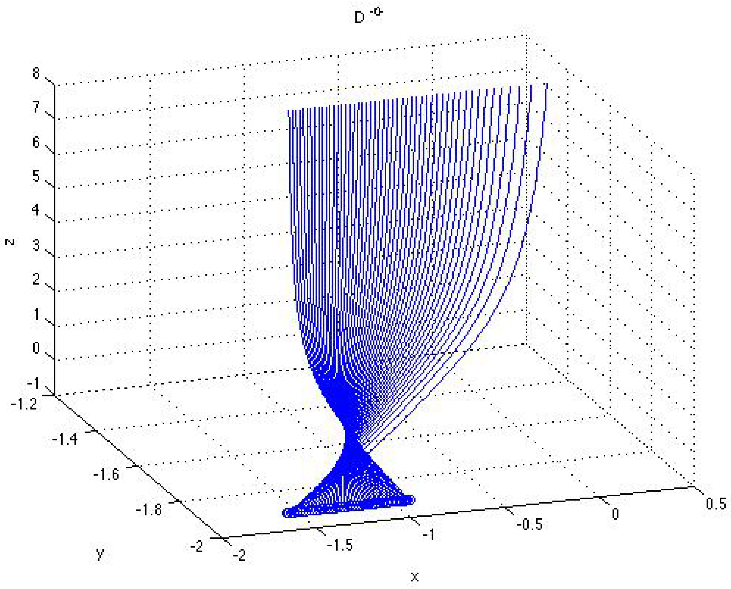
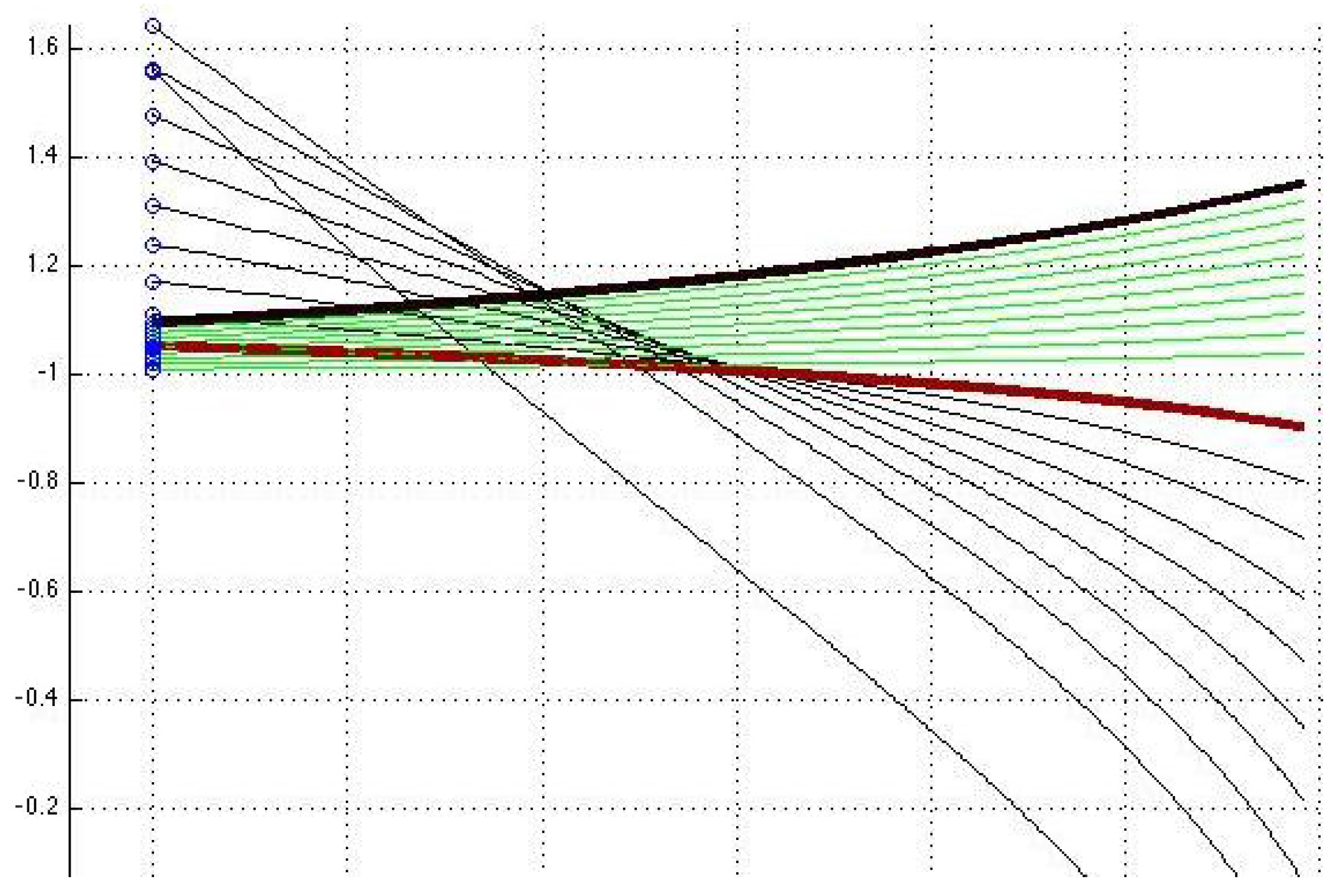
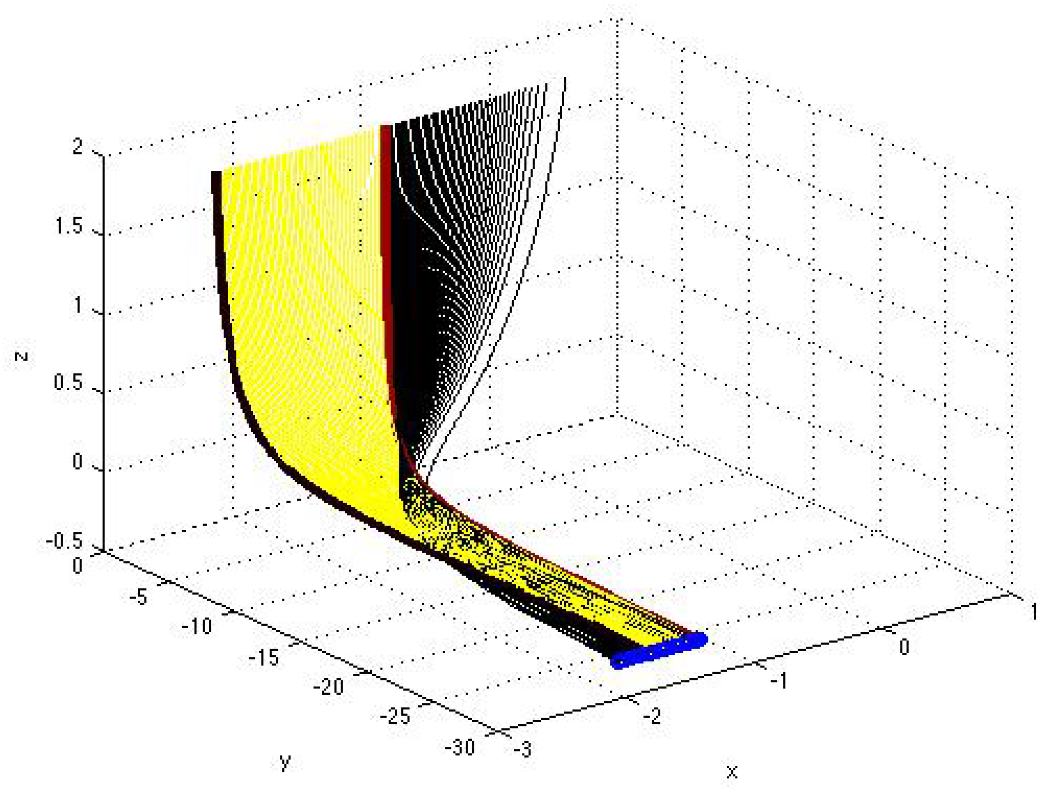
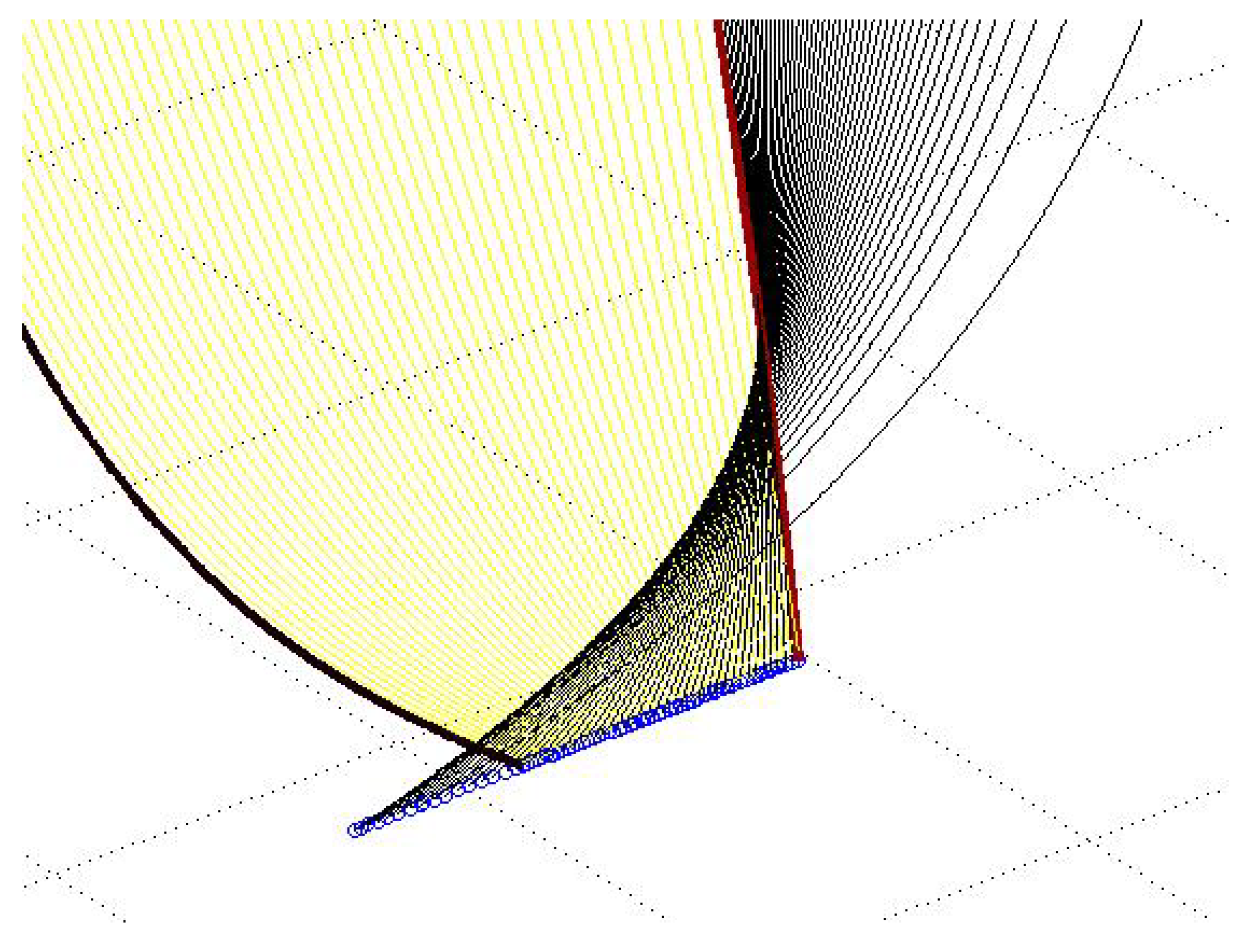
  • (b) D > 0; there are three solution families
    x t ; C = x 1 + D a 1 1 + C e D t , x 1 , 2 = x 0 ± D 2 a , x 0 = b 2 a , D = b 2 4 a c ,
    where the − and + signs correspond, respectively, to x 1 and x 2 :
    Family U, with C > 0 : solutions x t ; C = x U t ; C are not stable, since there is a “movable” singular point with t = t * C = ln C D ; next, they are (i) monotonically increasing because d x t ; C d t = D C e D t ( C e D t 1 ) 2 > 0 for C > 0; (ii) satisfy the condition x t ; C > x 2 , x < t * , x t ; C < x 1 , x > t * ; and (iv) have two horizontal asymptotes x = x 1 or x = x 2 .
    Family S, with C > 0 : solutions x t ; C = x S t ; C are stable and x 1 < x t ; C < x 2 .
    Family T, : x = x 1 and x = x 2 are time-independent solutions such that x 0 = x 1 o r x 0 = x 2 , and the first corresponds to C = 0 in x t ; C = x 1 + D a 1 1 + C e D t . These stationary solutions x = x 1 and x = x 2 are ’nonisolated’: in every neighborhood, there is an infinite number of ‘regular’ solutions x U t ; C or x S t ; C .
  • (c), D = 0 : all the corresponding solutions
    x t ; C = 1 a b 2 + 1 t C
    are not stable.
  • (d), D < 0 : the corresponding solutions
    x t ; C = x 0 + D 2 a tan D 2 t + C , D < 0 ,
    are not stable.
Note again all properties of the general solutions to autonomous second-order polynomial equation are fully described in [6].

3.3. Equivalence Classes of D-Vectors and General Solutions to Autonomous Polynomial Equation Systems

Summarize all possible combinations of general solutions to DS (42) of dimension three, identifying eight solution sets D + + + , D + + , D + + , D + , D + + , D + , D + , and D governed by all possible combinations of the non-zero discriminant signs. We identify as well 27 solutions to DS (42) of dimension three as sets D p m z , including all the above-defined eight solution sets, where p, m and z denote plus, minus, or zero and p m z is any of their combinations, including those with two or three repetitions, corresponding to all possible combinations of the zero and non-zero discriminant signs.
A set D p m z with a fixed combination p m z of signs is the equivalence class (defined in terms of S-vectors) in the sense that all its elements have the same S-vector S p m z .
These solution sets are presented below in the convenient form of matrices (47) and (48).
In what follows, we will consider the equations in system (42) with a i 1 0 , i = 1 , 2 , 3 . and make use of the function families
g + t ; D , C , a = D a 1 1 + C e D t , D > 0 ,
g 0 t ; C , a , b = 1 a b 2 + 1 t C , D = 0 ,
g t ; D , C , a = D 2 a tan D 2 t + C , D < 0 ,
where C is an arbitrary constant, specifying component-wise the general solutions of (42) for the respective signs of the discriminants D = D i = a i 2 2 4 a i 1 a i 3 of polynomials P i in system (42), i = 1 , 2 , 3 .

3.4. Description of All Possible Solution Combinations in Terms of Discriminants

In view of (43) and the relation between the coefficient matrix (17) and vectors (20), introduce the eight vector functions
g + + + = [ g + ( t ; D 1 , C 1 , a 11 ) , g + ( t ; D 2 , C 2 , a 21 ) , g + ( t ; D 3 , C 3 , a 31 ) ] , , g = [ g ( t ; D 1 , C 1 , a 11 ) , g ( t ; D 2 , C 2 , a 21 ) , g ( t ; D 3 , C 3 , a 31 ) ] ,
corresponding to the respective solution sets D + + + , …, D , so that the upper indices are the S-vectors that indicate the respective equivalence classes; the solution sets are formed by the vector functions
x + + + = x 1 + g + + + , or x t ; C 1 = x 1 + D 1 a 11 1 1 + C 1 e D 1 t , y t ; C 2 = y 1 + D 2 a 21 1 1 + C 2 e D 2 t , z t ; C 3 = z 1 + D 3 a 31 1 1 + C 3 e D 3 t ,
x = x 1 + g , or x t ; C 1 = x 1 + D 1 2 a tan D 1 2 t + C 1 , y t ; C 2 = y 1 + D 2 2 a tan D 2 2 t + C 2 , z t ; C 3 = z 1 + D 3 2 a tan D 3 2 t + C 3 ;
here
x 1 , 2 ( D 1 ) = x 0 ± D 1 2 a 11 , x 0 = a 12 2 a 11 , y 1 , 2 ( D 2 ) = y 0 ± D 2 2 a 21 , y 0 = a 22 2 a 21 , z 1 , 2 ( D 3 ) = z 0 ± D 3 2 a 31 , z 0 = a 32 2 a 31
a i 1 0 and D i > 0 , i = 1 , 2 , 3 .
The matrix
G ( + ) = g + + + g + + g + + g + g g + + g + g +
associated with DS (42) comprises all eight possible solution sets of system (42) corresponding to all possible combinations of the solution components having non-zero determinants and characterized by their S-vectors. Empty entries may be replaced by zeros.
The matrix
G ( + 0 ) = g + + + g + + g + g + + g + + 0 g + 0 g + + g + g g + g + 0 g 0 g 00 + g 00 g 000 g + 00 g 00 g 0 + 0 g 0 0 g + 0 + g 0 + + g 0 + g 0 + g + 0 g 0 + g 0 g 0
comprises all possible 27 solution sets of system (42) corresponding to all possible combinations with non-zero and zero determinants and characterized by their S-vectors. Empty entries in (48) may be replaced by zeros.

3.5. Analysis of Solutions to Cauchy Problems

Solutions to the Cauchy problems, e.g., to x ˙ = P 1 x , x 0 = q 0 , where polynomial P 1 x is given by (42), are
x t ; C 1 0 , + = x 1 + g + t ; D 1 , C 1 0 , + , a 11 = x 1 + D 1 a 11 1 1 + C 1 0 , + e D 1 t ,
C 1 0 , + = 1 + a 11 D 1 1 q 0 x 1
for D 1 > 0 and
x t ; C 1 0 , = x 0 + g t ; D 1 , C 1 0 , , a 11 = x 0 + D 1 2 a 11 tan D 1 2 t + C 1 0 , ,
C 1 0 , = 2 D 1 arctan 2 a 11 D 1 q 0 + x 0 , C 1 0 , π 2 + π n , n = 0 , ± 1 , ± 2 , ,
for D 1 < 0 , so that the solution to x ˙ = P x , x 0 = q 0 , q 0 = q 1 0 , q 2 0 , q 3 0 , can be written for different solution sets D + + + , …, D , as
x = x 1 + g + + + , or x t ; C 1 0 , + = x 1 + D 1 a 11 1 1 + C 1 0 , + e D 1 t , y t ; C 2 0 , + = y 1 + D 2 a 21 1 1 + C 2 0 , + e D 2 t , z t ; C 3 0 , + = z 1 + D 3 a 31 1 1 + C 3 0 , + e D 3 t ,
C i 0 , + = 1 + a i 1 D i 1 q i 0 x ( i ) , for D + + + , etc., where i = 1 , 2 , 3 , x ( 1 ) = x 1 , x ( 2 ) = y 1 , x ( 3 ) = z 1 .

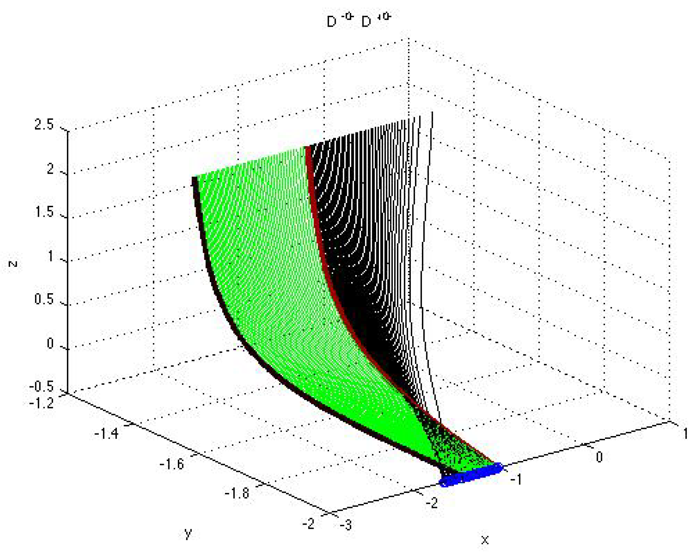
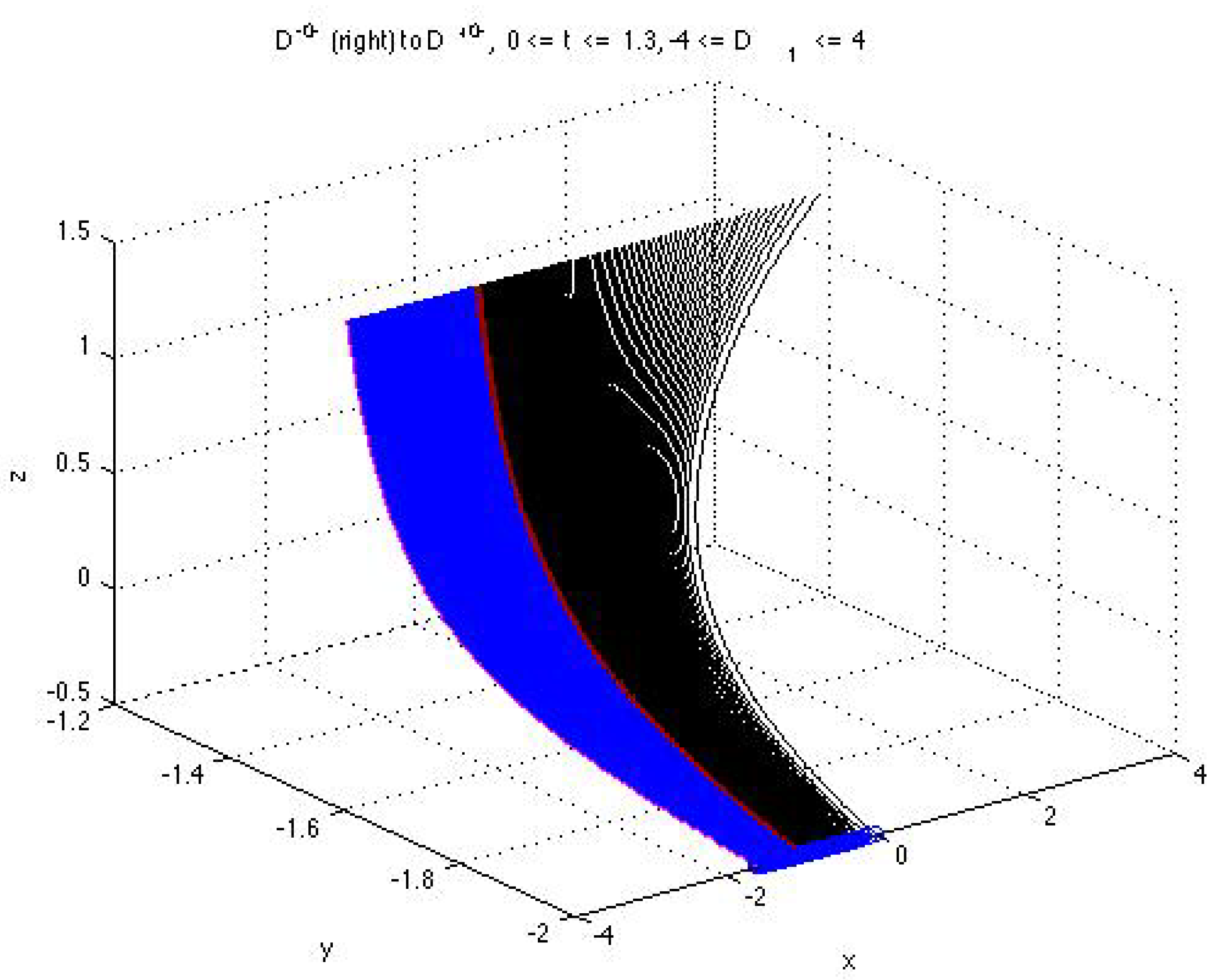
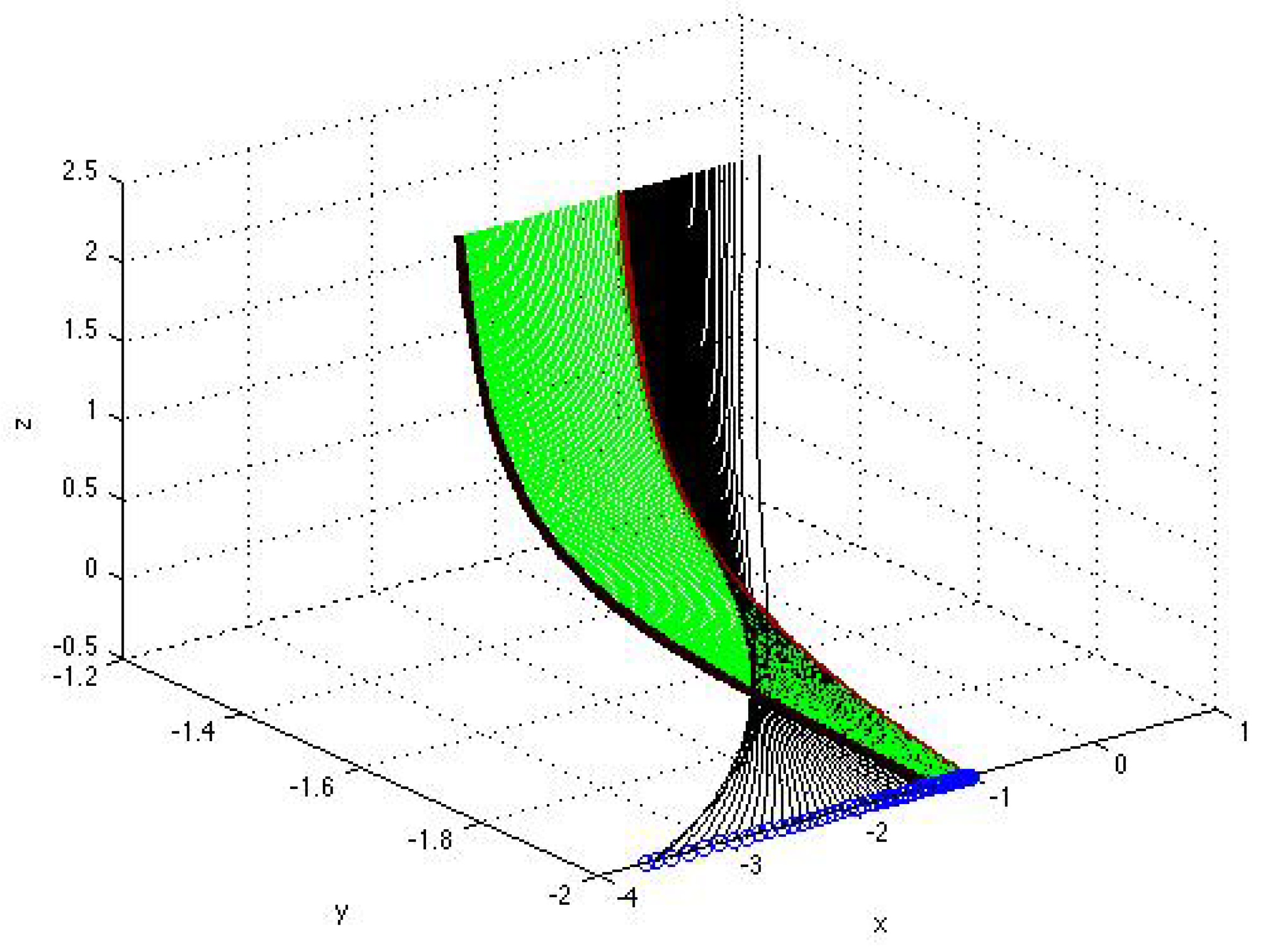
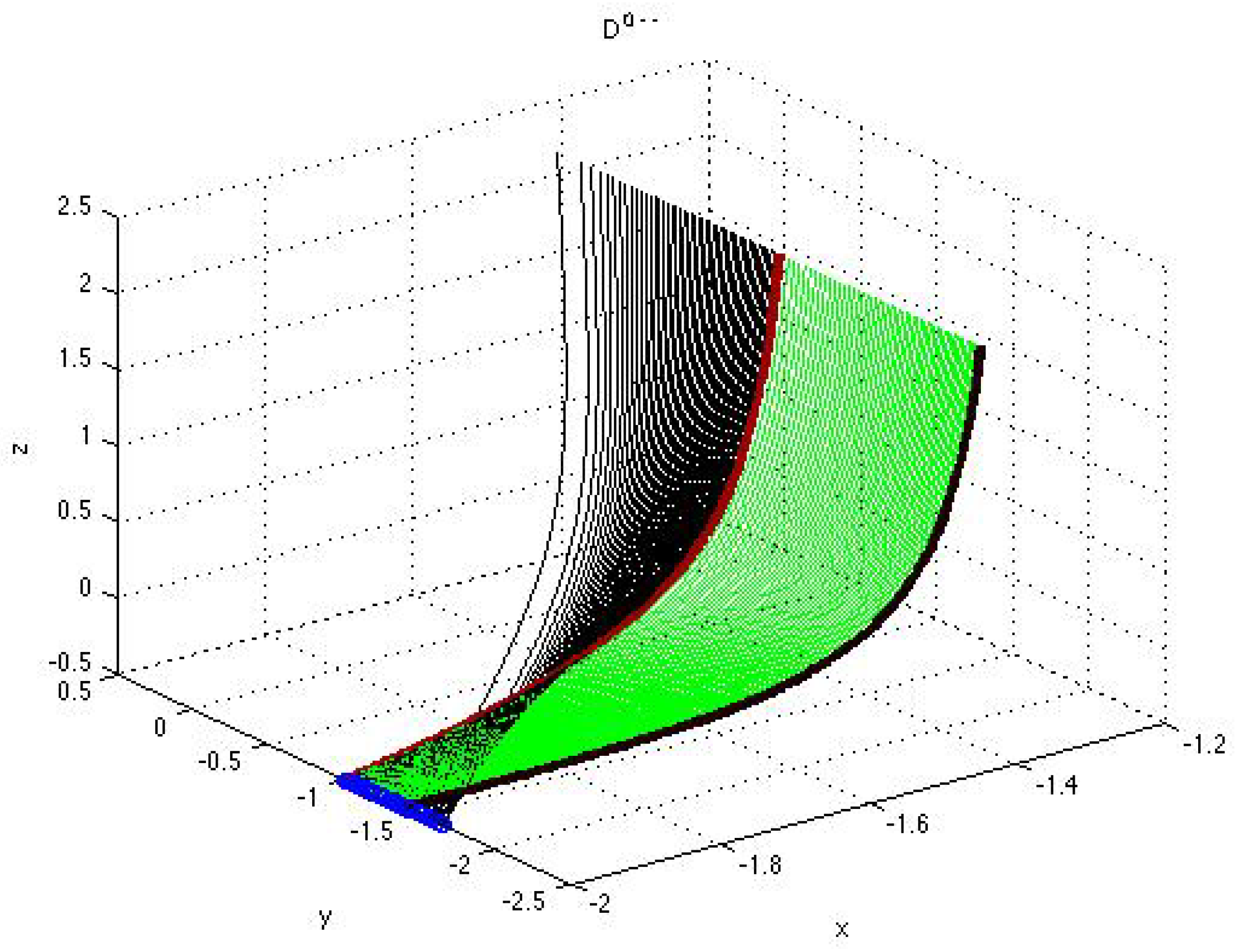
4. Analysis of Bifurcations

Families of vector functions x . . . ( t ; C ; D ) exemplified in (44) with C = C 1 , C 2 , C 3 C R 3 and D = D 1 , D 2 , D 3 D R 3 , where C, D, and . . . denote, respectively, certain 3D sets (or domains) and any combination of three signs +, − and 0, each specify a 3D surface X Ψ . . . formed by the corresponding curves x . . . ( t ; . ) parametrized by t T 0 , T 1 , T 0 0 and constructed for different values of one (the rest being fixed) real parameter Ψ = D j or Ψ = C j , j = 1 , 2 , 3 : X Ψ . . . = x . . . ( t ; Ψ ) , t T 0 , T 1 , Ψ Ψ 0 , Ψ 1 ; an example of such surface is presented in Figure 1.
We particularly investigate the occurrence of bifurcations for the combined surfaces X Ψ = D 1 0 X Ψ = D 1 + 0 when the discriminant of one (or two) component varies.
We have, according to (43),
lim D 1 + 0 x 0 ± D 1 2 a 11 + g + t ; D 1 , C , a 11 = x 0 ,
lim D 1 0 x 0 + g t ; D 1 , C , a 11 = x 0 ,
uniformity, with respect to t t 0 , T 0 , t 0 0 . The authors of (49) and (50) mean that there is no bifurcation associated with the transition D 0 D + 0 as illustrated by Figure 2.
Figure 2, Figure 3, Figure 4, Figure 5, Figure 6, Figure 7 and Figure 8 illustrate the formation of a bifuraction of the type-twisted fold (a ‘cusp’). This bifuraction occurs with the variation in discriminant D 1 of a single (first or second) solution component within single family D 0 or D 0 at certain values of constant C 1 (namely, at C 1 = 1 , 1.3 ) when the first and third (or the second and third) components (independent of variable D 1 ) are bounded in a closed interval t 0 , T 0 , where the parametrization is applied.
A twisted fold manifests itself as a ’rotation’ caused by a varied D 1 ( 4 , 0 ) of a 3D surface formed by the curves x 0 ( t ; D 1 ) or x 0 ( t ; D 1 ) , parametrized by t T 0 , T 1 , T 0 0 , with fixed vectors C = C 1 , C 2 , C 3 and D = D 1 , D 2 , D 3 and with constant D 2 and D 3 and varied D 1 . The ’rotation’ takes place around a point of equilibrium where all the curves x 0 ( t ; D 1 ) or x 0 ( t ; D 1 ) with different D 1 ( 4 , 0 ) merge at a certain t T 0 , T 1 .
To understand the nature of the observed bifurcation, consider system (42), corresponding to families D 0 , and the cases involving the specific values of parameters (coefficients of the trinomials in (42)) illustrated in Figure 3, Figure 5, Figure 9, and Figure 10.
x ˙ = ( x 1 2 D 1 + 4 ) 2 1 4 D 1 , y ˙ = ( y + 1 ) 2 , z ˙ = ( z 1 2 ) 2 + 3 4 ,
where D 1 < 0 and D 1 > 0 are, respectively, for D 0 and D + 0 . The second component in (51) has the degenerate stationary solution y = 1 , while the first and third components preserve the (positive) sign when parameter D 1 varies. Figure 11 displays the initial condition x ( 0 ) = D 1 + 4 2 D 1 2 tan D 1 2 vs. D 1 4 , 0 of the first component of the solution (A22), (A23) from the set D 0 presented in Figure 1. We see that the initial condition changes signs as D 1 < 0 increases, which causes a twist of the curves, contrary to the surface X D 1 0 X D 1 + 0 in Figure 2 where the solutions from the sets D 0 and D + 0 are given by (A16)–(A21) and the initial condition x ( 0 ) = D 1 + 4 2 for the first component considered vs. D 1 4 , 0 does not change signs and the solution curves in both sets D 0 and D + 0 preserve the same shape.

5. Conclusions

We have extended the discriminant criterion applied originally to two-phase quadratic polynomial DSs to three-phase DSs investigated in terms of their coefficient matrices. Based on this criterion and the established integrability in elementary functions for the considered class of autonomous polynomial DSs, we have proposed a general approach to qualitative analysis of these DSs. Specific classes of D- and S-vectors have been introduced which enable one to classify the DS solutions depending on the discriminant signs. Complete description of the symmetry relations inherent to the DS coefficient matrices has been performed using the discriminant criterion. The DS solution properties have been investigated in terms of two-parameter surfaces. The behavior and bifurcations of solutions to three-dimensional quadratic polynomial DSs have been considered. The occurrence of bifurcations of the type-twisted fold has been discovered on the basis and within the frames of the developed DS qualitative theory.
Based on the results of the study, we have made the following conclusion: whether the DS coefficient matrix belongs to a particular equivalence class determines the presence and nature (type) of singular points and bifurcations of the corresponding polynomial DS.
Based on the results of this research and a big amount of computations, we can formulate a conjecture (to be proved) that the only type of bifurcations that may occur in 3D quadratic polynomial DSs investigated in this paper is the discovered ‘twisted fold’. This is a remarkable feature of this class of DSs. However, a complete proof of this statement goes far beyond the scope of this paper and may be technically rather difficult (as suggested by similar proofs and findings concerning the classification of bifurcations and critical points published by many authors, revised briefly in Section 2.1). In addition to this, we cannot provide a substantiated report concerning the type of singular points and bifurcations that are observed for each of the identified equivalence classes. We will continue our studies in this direction using the accumulated technical data and will report the results in the following publications.
Indicate in this respect main directions of the planned future research:
-
To develop the method of S- and D-vectors and the discriminant criterion to the polynomial DSs of higher dimensions and the order of the involved polynomials.
-
To clarify that the only type of bifurcations that may occur in quadratic polynomial DSs investigated in this paper is the discovered ‘twisted fold’.
-
To investigate the relations between the described symmetries of the D- and S-vectors and the possible symmetries of solutions to the polynomial DSs.
-
To find the symmetry-breaking bifurcations characteristic to the polynomial DSs under study.
As far as the application of the developed approach and technique to regulating and monitoring the waterflooding and the development of oil or gas fields is concerned, the proposed approach enables one to simulate the consequences of unstable behavior of the displacement front.
Using the results of this work, engineers and practitioners will be able to predict the blunt variations in water saturation and well exploitation data by applying the developed growth model that employs three-phase quadratic polynomial DSs.
The results and findings reported in this study make it possible to carry out systematic improvement in handling real-time waterflooding and to control a decrease in the water volume that is not properly put into action and pumped out.

Author Contributions

Conceptualization, Y.S. and A.S.; methodology, A.S.; software, Y.S. and A.S.; validation, Y.S., A.S. and S.V.A.; formal analysis, Y.S.; investigation, Y.S. and A.S.; resources, A.S. and S.V.A.; data curation, A.S. and S.V.A.; writing—original draft preparation, Y.S.; writing—review and editing, Y.S.; visualization, Y.S.; supervision, A.S. and S.V.A.; project administration, A.S. and S.V.A.; funding acquisition, A.S. All authors have read and agreed to the published version of the manuscript.

Funding

This research received no external funding.

Data Availability Statement

No new data were created.

Conflicts of Interest

The authors declare no conflict of interest.

Appendix A

Appendix A.1. Autonomous Polynomial Dynamical Systems Integrable in Elementary Functions

A polynomial P i ( x ) of degree N i 2 ( i = 1 , 2 , , n ) with real coefficients can be uniquely factorized and represented as
P i ( x ) = Π s = 1 m i ( x x s ( i ) ) k s ( i ) Π t = 1 n i ( r t ( i ) ) p t ( i ) ,
where s = 1 m i k s ( i ) + 2 t = 1 n i p t ( i ) = N i , m i , n i 0 , and
r s ( i ) ( x ) = a s , 1 ( i ) x 2 + a s , 2 ( i ) x + a s , 3 ( i ) = a s , 1 ( i ) ( x + x s , 0 ( i ) ) 2 D s ( i ) 4 ( a s , 1 ( i ) ) 2 ( a s , 1 ( i ) 0 )
are irreducible quadratic trinomials with x s , 0 ( i ) = a s , 2 ( i ) 2 a s , 1 ( i ) and the discriminants
D s ( i ) = ( a s , 2 ( i ) ) 2 4 a s , 1 ( i ) a s , 3 ( i ) < 0 , s = 1 , 2 , , n i , i = 1 , 2 , , n .
A rational function Q i ( x ) = P i 1 ( x ) can be uniquely decomposed [20] into partial fractions,
Q i ( x ) = s = 1 m i j = 1 k s ( i ) A s j ( i ) ( x x s ( i ) ) j + t = 1 n i j = 1 p t ( i ) B t j ( i ) x + C t j ( i ) ( r t ( i ) ) j
where A s j ( i ) , B t j ( i ) , and C t j ( i ) are uniquely determined real numbers.
Lemma A1. 
Each term in (A4) is integrable in elementary functions.
Proof. 
Verification of the statement is obvious for the terms entering the first double sum in (A4).
Consider the terms entering the second double sum in (A4). To prove the required integrability, it is sufficient to calculate two indefinite integrals
I j ( 1 ) ( x ) = x d x r j ( x ) and I j ( 2 ) ( x ) = d x r j ( x ) , r ( x ) = a x 2 + b x + c ,
with integer j 1 and D = b 2 4 a c < 0 . For the first integral, we have
I j ( 1 ) ( x ) = x d x a ( x + x 0 ) 2 D 4 a 2 j = = 1 2 a j ( j 1 ) 1 ( x + x 0 ) 2 D 4 a 2 j 1 x 0 a j I j ( 2 ) ( x )
for j 2 and
I 1 ( 1 ) ( x ) = 1 a x d x ( x + x 0 ) 2 D 4 a 2 =
= 1 2 a ln ( x + x 0 ) 2 D 4 a 2 x 0 a I 1 ( 2 ) ( x ) = = 1 2 a ln ( x + x 0 ) 2 D 4 a 2 2 x 0 D tan 1 2 a ( x + x 0 ) D + C
for j = 1 . For the second integral, we have for j 2 ,
I j ( 2 ) ( x ) = 2 a x + b ( j 1 ) D r j 1 ( x ) 2 a ( 2 j 3 ) ( j 1 ) D I j 1 ( 2 ) ( x ) .
This is actually a first-order inhomogeneous difference equation which can be written in a compact form
I j ( 2 ) = α j 1 I j 1 ( 2 ) + β j 1 , j = 2 , 3 , , I 1 ( 2 ) = 2 a D tan 1 2 a ( x + x 0 ) D ,
The solution to (A10) is
I j ( 2 ) = s = 1 j β j s Π t = 1 s α j t + 1 + I 1 ( 2 ) Π t = 1 j α t ,
where
α j 1 = 2 a x + b ( j 1 ) D r j 1 ( x ) , β j 1 = 2 a ( 2 j 3 ) ( j 1 ) D .
Thus, both I j ( 1 ) and I j ( 2 ) are expressed in elementary functions using (A11) and (A12). The indefinite integral
Q i ( x ) d x = s = 1 m i j = 1 k s ( i ) A s j ( i ) q j , s ( i ) ( x ) + T i ( x ) ,
where
q j , s ( i ) ( x ) = 1 ( j 1 ) ( x x s ( i ) ) j 1 , j 2 , ln x x s ( i ) , j = 1 ,
and T i ( x ) is a linear combination of I j ( 1 ) and I j ( 2 ) which proves the lemma. □
Theorem A1. 
DSs (41) (and (42)) are integrable in elementary functions.
Proof. 
Each particular row equation in (41) is written as
d x d t = P i x , P i x = j = 1 N i + 1 a j i x N i j + 1 = = a 1 i x N i + a 2 i x N i 1 + + a N i , i x + a N i + 1 , i ( i = 1 , 2 , , n )
yields a rational function Q i ( x ) = P i 1 ( x ) , which is uniquely decomposed into partial fractions (A4) and is therefore integrable in elementary functions according to Lemma A1.

Appendix A.2. Examples with Bifurcations

Parametrized curves x ( t ; D 1 ) = x 1 + g 0 , 4 < D 1 < 0 , and x ( t ; D 1 ) = x 1 + g + 0 , 0 < D 1 < 4 for 0 t 1.3 , forming surface X D 1 0 X D 1 + 0 , corresponding to the solutions from the sets D 0 and D + 0 displayed in Figure 2
x 0 = x 1 + g 0 =
x t ; C 1 = 0 = x 0 + g t ; D 1 , C 1 = 0 , 1 y t ; C 2 = g 0 t ; C 2 = 1 , a 21 , a 22 , z t ; C 3 = z 0 + g t ; D 3 = 3 , C 3 = 0 , 1 , =
= D 1 + 4 a 11 a 13 2 a 11 + D 1 2 a 11 tan D 1 2 t , 1 a 21 a 22 2 + 1 t C 2 , D 3 + 4 a 31 a 33 2 a 31 + D 3 2 a 31 tan D 3 2 t , = 1 2 D 1 + 4 + D 1 2 tan D 1 2 t , 1 1 t + 1 , 1 2 + 3 2 tan 3 2 t .
x + 0 = x 1 + g + 0 =
x t ; C 1 = 1 = x 1 + D 1 a 11 1 1 + C 1 e D 1 t , y t ; C 2 = g 0 t ; C 2 = 1 , a 21 , a 22 , z t ; C 3 = z 0 + g t ; D 3 = 3 , C 3 = 0 , 1 , =
= D 1 + 4 a 11 a 13 2 a 11 + D 1 2 a 11 + D 1 a 11 1 1 + C 1 e D 1 t , 1 a 21 a 22 2 + 1 t C 2 , D 3 + 4 a 31 a 33 2 a 31 + D 3 2 a 31 tan D 3 2 t , = 1 2 D 1 + 4 D 1 1 + e D 1 t , 1 1 t + 1 , 1 2 + 3 2 tan 3 2 t .
Parametrized curves x ( t ; D 1 ) = x 1 + g 0 , C 1 = 1 , 4 < D 1 < 0 , and x ( t ; D 1 ) = x 1 + g + 0 , 0 < D 1 < 4 , for 0 t 1.3 with a 11 = a 13 = a 21 = 1 and a 22 = 2 forming surface X D 1 0 X D 1 + 0 corresponding to the solutions from the sets D 0 and D + 0 displayed in Figure 1
x 0 = x 1 + g 0 =
x t ; C 1 = 1 = x 0 + g t ; D 1 , C 1 = 1 , 1 y t ; C 2 = g 0 t ; C 2 = 1 , a 21 , a 22 , z t ; C 3 = z 0 + g t ; D 3 = 3 , C 3 = 0 , 1 , =
= D 1 + 4 a 11 a 13 2 a 11 + D 1 2 a 11 tan D 1 2 ( t 1 ) , 1 a 21 a 22 2 + 1 t C 2 , D 3 + 4 a 31 a 33 2 a 31 + D 3 2 a 31 tan D 3 2 t , = 1 2 D 1 + 4 + D 1 2 tan D 1 2 ( t 1 ) , 1 1 t + 1 , 1 2 + 3 2 tan 3 2 t ,
x + 0 = x 1 + g + 0 =
= x t ; C 1 = 1 = x 1 + D 1 a 11 1 1 + C 1 e D 1 t , y t ; C 2 = g 0 t ; C 2 = 1 , a 21 , a 22 , z t ; C 3 = z 0 + g t ; D 3 = 3 , C 3 = 0 , 1 , =
= D 1 + 4 a 11 a 13 2 a 11 + D 1 2 a 11 + D 1 a 11 1 1 + C 1 e D 1 t , 1 a 21 a 22 2 + 1 t C 2 , D 3 + 4 a 31 a 33 2 a 31 + D 3 2 a 31 tan D 3 2 t , = 1 2 D 1 + 4 D 1 1 + e D 1 t , 1 1 t + 1 , 1 2 + 3 2 tan 3 2 t .

References

  1. Gaiko, V.A. Global bifurcations and chaos in polynomial dynamical systems. In Proceedings of the 2003 International Conference Physics and Control. Proceedings, St. Petersburg, Russia, 20–22 August 2003; Volume 2, pp. 670–674. [Google Scholar] [CrossRef]
  2. Gaiko, V.A. Global Bifurcation Theory and Hilbert’s Sixteenth Problem. In Book Series: Mathematics and Its Applications; Kluwer: Boston, MA, USA, 2003; Volume 562. [Google Scholar]
  3. Luo, A. Polynomial Functional Dynamical Systems, E-Book; Springer International Publishing: Berlin/Heidelberg, Germany, 2022. [Google Scholar]
  4. Bautin, N.N.; Leontovich, E.A. Methods and Examples of the Qualitative Analysis of Dynamical Systems in a Plane; Nauka: Moscow, Russia, 1990. [Google Scholar]
  5. Gaiko, V.A. On Global Bifurcation Theory of Polynomial Dynamical Systems and Its Applications. In Communications in Difference Equations; CRC Press: Boca Raton, FL, USA, 2000. [Google Scholar] [CrossRef]
  6. Shestopalov, Y.V.; Shakhverdiev, A.K. Qualitative theory of two-dimensional polynomial dynamical systems. Symmetry 2021, 13, 1884. [Google Scholar] [CrossRef]
  7. Buckley, I.; Leverett, M.C. Mechanism of Fluid Displacement in Sands. Trans. AIME 1942, 146, 107–119. [Google Scholar] [CrossRef]
  8. Suleimanov, B.A.; Guseynova, N.I.; Veliyev, E.F. Control of Displacement Front Uniformity by Fractal Dimensions. In Proceedings of the SPE-187784-MS, SPE Russian Petroleum Technology Conference, Moscow, Russia, 16–18 October 2017. [Google Scholar] [CrossRef]
  9. Suleimanov, B.A.; Veliyev, E.F.; Naghiyeva, N.V. Preformed particle gels for enhanced oil recovery. Int. J. Mod. Phys. B 2020, 34, 2050260. [Google Scholar] [CrossRef]
  10. Shakhverdiev, A.K. System optimization of non-stationary flooding for the purpose of increasing oil recovery. Pet. Eng. 2019, 44–49. [Google Scholar] [CrossRef]
  11. Shakhverdiev, A.K.; Arefiev, S.V.; Denisov, A.V.; Yunusov, R.R. Method for restoring the optimal mode of operation of the reservoir-well system, taking into account the instability of the displacement front. Oil Ind. 2020, 6, 52–57. [Google Scholar] [CrossRef]
  12. Shakhverdiev, A.K.; Arefiev, S.V. The concept of monitoring and optimization of oil reservoirs waterflooding under the conditions of displacement front instability. Oil Ind. 2021, 11, 104–109. [Google Scholar] [CrossRef]
  13. Shakhverdiev, A.K. Once again about oil recovery factor. Neft. Khozyaystvo 2014, 1, 44–48. [Google Scholar]
  14. Drozdov, A.N.; Gorelkina, E.I. Method of measuring the rates of water-gas mixtures injection wells during the exploitation of oil fields. Socar Proc. 2022, 1–8. [Google Scholar] [CrossRef]
  15. Suleimanov, B.A.; Ismailov, F.S.; Dyshin, O.A.; Veliyev, E.F. Selection methodology for screening evaluation of EOR methods. Pet. Sci. Technol. 2016, 34, 961–970. [Google Scholar] [CrossRef]
  16. Craig Forrest, F., Jr. The Reservoir Engineering Aspects of Waterflooding; Society of Petroleum Engineers of AIME: New York, NY, USA, 1971. [Google Scholar]
  17. Dake, L.P. The Practice of Reservoir Engineering; Shell Internationale Petroleum Maatschappij B.V.: The Hague, The Netherlands, 2001. [Google Scholar]
  18. Constantinescu, D. On the Bifurcations of a 3D Symmetric Dynamical System. Symmetry 2023, 15, 923. [Google Scholar] [CrossRef]
  19. Fenichel, N. Geometric Singular Perturbations Theory for Ordinary Differential Equations. J. Differ. Equ. 1979, 31, 53–98. [Google Scholar] [CrossRef]
  20. Bradley, W.T.; Cook, W.J. Two Proofs of the Existence and Uniqueness of the Partial Fraction Decomposition. Int. Math. Forum 2012, 7, 1517–1535. [Google Scholar]
Figure 1. Surface X D 1 0 X D 1 + 0 formed by the parametrized curves x ( t ; D 1 ) = x 1 + g 0 (black), C 1 = 1 , 4 < D 1 < 0 , and x ( t ; D 1 ) = x 1 + g + 0 , 0 t 1.3 (green), 0 < D 1 < 4 , with a 11 = a 13 = a 21 = 1 and a 22 = 2 given by (43)–(46) corresponding to the solutions from the sets D 0 and D + 0 . The explicit formulas (A22)–(A26) for the parametrized components are in Appendix A.
Symmetry 16 00014 g001
Figure 2. Surface X D 1 0 X D 1 + 0 formed by the parametrized curves x ( t ; D 1 ) = x 1 + g 0 (right, black), 4 < D 1 < 0 , and x ( t ; D 1 ) = x 1 + g + 0 , 0 t 1.3 (left, blue), 0 < D 1 < 4 , with a 11 = a 13 = a 21 = 1 and a 22 = 2 given by (43)–(46) corresponding to the solutions from the sets D 0 and D + 0 . The explicit formulas (A16)–(A21) for the parametrized components are in Appendix A.
Symmetry 16 00014 g002
Figure 3. Surface X D 1 0 X D 1 + 0 formed by the parametrized curves x ( t ; D 1 ) = x 1 + g 0 (black), C 1 = 1.3 , 4 < D 1 < 0 , and x ( t ; D 1 ) = x 1 + g + 0 , 0 t 1.3 (green), 0 < D 1 < 4 , with a 11 = a 13 = a 21 = 1 and a 22 = 2 given by (43)–(46) corresponding to the solutions from the sets D 0 and D + 0 .
Symmetry 16 00014 g003
Figure 4. Surface X D 1 0 X D 1 + 0 formed by the parametrized curves x ( t ; D 1 ) = x 1 + g 0 (black), C 1 = 1 , 4 < D 1 < 0 , and x ( t ; D 1 ) = x 1 + g + 0 , 0 t 1.3 (green), 0 < D 1 < 4 , with a 11 = a 13 = a 21 = 1 and a 22 = 2 given by (43)–(46) corresponding to the solutions from the sets D 0 and D + 0 .
Symmetry 16 00014 g004
Figure 5. Surface X D 1 0 formed by the parametrized curves x ( t ; D 1 ) = x 1 + g 0 , 0 t 1.45 , 2 D 1 < 0 , a 11 = a 13 = 1 given by (43)–(46) corresponding to the solutions from the set D 0 .
Symmetry 16 00014 g005
Figure 6. Enlarged fragment of the projection on the ( x , y ) -plane of the surface, presented in Figure 4, close to the point of bifuraction associated with the stationary solution y = 1 of the second component in system (51) (graphs of the parametrized curves x ( t ) = x 1 + g 0 (black), C 1 = 1 , 4 < D 1 < 0 , and x ( t ) = x 1 + g + 0 , 0 t 1.3 (green), 0 < D 1 < 4 , with a 11 = a 13 = a 21 = 1 and a 22 = 2 given by (43)–(46) corresponding to the solutions from the sets D 0 and D + 0 ).
Symmetry 16 00014 g006
Figure 7. Graphs of the parametrized curves x ( t ; D 1 ) = x 1 + g 0 (black), C 1 = 1 , C 2 = 0.04 , 4 < D 1 < 0 , and x ( t ; D 1 ) = x 1 + g + 0 , 0 t 1.4 (yellow), 0 < D 1 < 4 , with a 11 = a 13 = a 21 = 1 and a 22 = 2 given by (43)–(46) corresponding to the solutions from the sets D 0 and D + 0 .
Symmetry 16 00014 g007
Figure 8. Enlarged fragment of the surface close to the point of bifuraction associated with the stationary solution y = 1 of the second and third components in system (51) (graphs of the parametrized curves x ( t ; D 1 ) = x 1 + g 00 (black), C 1 = 1 , 4 < D 1 < 0 , C 2 = 1.6 , C 3 = 2 , and x ( t ; D 1 ) = x 1 + g + 00 , 0 t 1.5 (yellow), 0 < D 1 < 4 , with a 11 = a 13 = a 21 = 1 and a 22 = 2 given by (43)–(46) corresponding to the solutions from the sets D 00 and D + 00 ).
Symmetry 16 00014 g008
Figure 9. Graphs of the parametrized curves x ( t ) = x 1 + g , 0 t 2 , 4 D 1 , D 3 < 0 , a 11 = a 13 = 1 , a 22 = a 32 = 2 , C j = 1 , j = 1 , 2 , 3 , given by (43)–(46) corresponding to the solutions from the set D with two variable components.
Symmetry 16 00014 g009
Figure 10. Graphs of the parametrized curves x ( t ) = x 1 + g + (right) and x ( t ) = x 1 + g + + , 0 t 1.3 , 4 D 1 6 , a 11 = a 13 = 1 given by (43)–(46) corresponding to the solutions from the sets D + and D + + .
Symmetry 16 00014 g010
Figure 11. Graph of the initial condition x ( 0 ) = D 1 + 4 2 D 1 2 tan D 1 2 vs. D 1 4 , 0 of the first component of the solution (A22), (A23) from the set D 0 presented in Figure 1.
Symmetry 16 00014 g011
Disclaimer/Publisher’s Note: The statements, opinions and data contained in all publications are solely those of the individual author(s) and contributor(s) and not of MDPI and/or the editor(s). MDPI and/or the editor(s) disclaim responsibility for any injury to people or property resulting from any ideas, methods, instructions or products referred to in the content.

