Integrated Approach to Obtain Gas Flow Velocity in Convection Reflow Soldering Oven

Abstract

The nozzle-matrix gas flow velocity has a great influence on the accuracy of the temperature field of a printed circuit board assembly (PCBA) during the hot air convection reflow soldering process. This paper proposes a new approach that integrates the theoretical calculation, numerical simulation and an experimental test to accurately determine the nozzle-matrix gas flow velocity. First, the temperature profile of the aluminum alloy thin plate in convection reflow ovens is measured using a Wiken tester. Second, the nozzle-matrix gas flow velocity is theoretically calculated with the Martin formula. The computational fluid dynamic (CFD)simulation is performed according to the Icepak code, where a single oven chamber model is established to represent the 10 zones of soldering ovens to reduce computational resources considering the supry of the soldering ovens. The simulated temperature profile of the aluminum alloy thin plate is obtained and the specific response surface model (RSM) is established to represent the deviation between the simulated temperature and the measured temperature. Finally, based on reverse problem analysis, non-linear programming by quadratic Lagrangian (NLPQL) is used to solve the mathematical optimization model with the objective of minimizing the temperature deviation to obtain the corrected nozzle-matrix gas flow velocity. To validate the accuracy, the temperature test and the modeling using the corrected gas flow velocity for a new PCBA component for the soldering ovens is conducted separately. The temperature comparison between the simulation and the test shows that the maximum temperature deviation is within 10 °C. This provides evidence that the nozzle-matrix gas flow velocity obtained by the new approach is accurate and effective.

1. Introduction

The hot air reflow soldering process is one of the most commonly used soldering processes in industry for printed circuit board assembly (PCBA) of electronic products. Typically, surface mount technology (SMT) assembly mainly includes four basic processes: printing, mounting, soldering and overhaul. Among these processes, reflow soldering is a key process, which directly affects the soldering quality and reliability of the electronic products [1]. In the reflow soldering process, the reflow oven heats the air, and then uses the fan to force the hot air to flow into the zone and heat the PCBA component. The heat transfer between the reflow oven and the PCBA component consists mainly of the convective heat transfer of the air and the heat radiation from the inner cavity of the heating oven to the PCBA component [2]. The common heater module of the reflow oven is shown in Figure 1. Hot air reflow soldering process parameters, including the temperature of each temperature zone, the transmission speed of the conveyor belt and the air volume should be setup in hot air reflow soldering [3]. These process parameters are critical for the reliability of the PCBA. As the product volume becomes smaller, the package density of PCB components becomes higher, the heat capacity distribution becomes more complicated, and the process design of the hot air reflow soldering becomes more challenging.

In engineering, the current process parameter design of the hot air reflow soldering process is dependent on multiple temperature tests, which require a large amount of manpower, material resources and time. Moreover, for PCBA products such as aerospace products that cannot afford to be tested several times, this method is unavailable. In these cases, a numerical simulation-based approach for the PCBA reflow soldering process has become an important and essential method due to its inherent advantages such as relative short time, low cost and no consumption of the physical products. There are several ways to simulate the reflow soldering process, including the finite element method (FEM) [4], finite volume method (FVM) [5,6], fluid-structure interface (FSI) [7], lattice Boltzmann’s method (LBM) [8], discrete phase method (DPM) [9] and molecular dynamic (MD) [10]. Whall et al. [11] used ANSYS finite element analysis software to conduct temperature field simulation of 2-D PCBA components and obtained simulated temperature data. Gong et al. [12] simulated the reflow soldering process and optimized the temperature profile by establishing the FE model of PCBA assembly containing a ball grid array (BGA) component and genetic algorithm (GA) optimization. Srivalli et al. [13] performed a numerical simulation of leadless reflow soldering based on the actual size in Fluent software to study the influence of cooling period on solder joint quality during reflow soldering. Iqbal et al. [14] established a 3-D model of the single-temperature zone of the reflow oven in Fluent software by developing a user-defined function (UDF) script with C++ language and adopting a 3-D, incompressible, unsteady turbulent flow pattern. Lai et al. [15,16] proposed a computational fluid dynamics (CFD)-based machine learning (ML) model to set the temperature of a convection reflow oven and control conveyor speed. Deng et al. [17] studied the real reflow soldering process based on Fluent moving mesh technology. Although a large amount of simulation has been conducted on the temperature field of the hot air reflow soldering process and shows great advantages, the accuracy of the model and simulation is a main concern and constrains its application in engineering. Especially for the complicated PCBA, the temperature estimated by the simulation during the hot air reflow soldering process deviates much from the temperature reached by the test and cannot meet the industry requirements of the process design. Theoretically, during the convection reflow soldering process, for the specific PCBA materials and structure, the PCBA temperature field is mainly determined by the gas flow temperature and gas flow velocity at the nozzle-matrix. These two factors represent the amount of heat supplied to the PCBA. Thus, the accuracy of these two parameters in the numerical model dominates the accuracy of the result of the simulation. Generally, several thermocouples are installed at the zone near the inlet to monitor the nozzle-matrix gas flow temperature, and thus the real-time values of nozzle-matrix gas flow temperature can be obtained with a high resolution. The accuracy of the nozzle-matrix gas flow temperature can be considered to be satisfied. However, the nozzle-matrix gas flow velocity at the inlet is not measured instantly, and the actual value of the inlet velocity is unclear. On many occasions, the real-time value of nozzle-matrix gas flow velocity may change significantly from its initial value, especially as the reflow oven works for a relatively long period of time. Therefore, accurately obtaining the nozzle-matrix gas flow velocity value at the inlet is very critical for the accurate modeling and simulation of hot air reflow soldering process. Due to the extreme circumstances in the reflow oven, it is difficult to test the dynamic nozzle-matrix gas flow velocity [18]. The industry demands a reliable and easy way to obtain nozzle-matrix gas flow velocity which becomes, in fact, a bottleneck problem in hot air reflow soldering process.

This paper proposes a new approach to obtain an accurate value of the nozzle-matrix gas flow velocity, which can easily be performed in the industry and provides high accuracy based on the numerical simulation and heat transfer reverse problem analysis theory.

2. Integrated Approach

2.1. Basic Concept of the Approach

The basic process of this approach consists of four steps: establishing a simulation model of the reflow process, determining experimental design, constructing response surface model and optimizing. The approach here includes parameter sensitivity analysis, design of experiment (DoE), response surface fitting and goodness-of-fit testing. The flowchart of this approach is shown in Figure 2.

2.2. Theoretical Calculation of Nozzle-Matrix Gas Flow Velocity

During the reflow soldering process, one motor at the top of the temperature zone and the other motor at the bottom of the temperature zone drive the fan to rotate at high speed, thereby generating air blowing force [19]. After the inhaled gas flows through the heating tube, it becomes a gas with a certain high temperature and passes through the porous cover and then blows to the PCB board. According to its heating principle, each nozzle outlet presents an impact jet process. The nozzle heating structure of each temperature zone is shown in Figure 3 [19].

H. Martin summarizes the results of the impact jet convection coefficient where the nozzle outflow appears as an impact jet [20,21]. The average Nusselt number in the Martin formula can be calculated with the following Equations (1)–(3):

$$\overline{Nu}=f(\mathrm{Re},\mathrm{Pr},A_r,H/D)$$

(1)

$$\overline{N_u}=\frac{D\overline{h}}{k}$$

(2)

$$\mathrm{Re}=\frac{V_{e}D}{\nu }$$

(3)

For nozzle arrays in a positive hexagonal arrangement, the relative orifice area A_r is as follows:

$$A_r=\frac{\pi }{2\sqrt{3}}{\left(\frac{D}{S}\right)}^2$$

(4)

Therefore, according to H. Martin’s research on the impact jet, the recommended correlation formula of Nusselt number is as shown in Equations (5) and (6):

$$\overline{N_u}=\frac{0.5G{\mathrm{Pr}}^{0.42}{\mathrm{Re}}^{\frac{2}{3}}}{{\left[1+{\left(\frac{H}{D}\frac{\sqrt{A_r}}{0.6}\right)}^6\right]}^{0.05}}$$

(5)

$$G=2\sqrt{A_r}\frac{1-2.2\sqrt{A_r}}{1+0.2(\frac{H}{D}-6)\sqrt{A_r}}$$

(6)

The scope of application of this formula is as follows:

$$\left[\begin{array}{c}2\times {10}^3\le \mathrm{Re}\le {10}^5\\ 2\le H/D\le 12\\ 0.004\le A_r\le 0.04\end{array}\right]$$

Define K as a new variable:

$$K={\left[1+{\left(\frac{H}{D}\frac{\sqrt{A_r}}{0.6}\right)}^6\right]}^{0.05}$$

(7)

$$\delta =\frac{0.5GK}{D^{\frac{1}{3}}}$$

(8)

As can be seen from Equation (8), δ is a constant, and it is only related to the layout, diameter and distance between the nozzles.

Finally, according to Equations (1)–(8), the theoretical nozzle-matrix gas flow velocity of the reflow oven can be obtained as follows [17,18]:

$$V_{\mathrm{e}}={\left[\frac{1}{\delta k{\mathrm{Pr}}^{0.42}}\right]}^{\frac{3}{2}}\nu {\overline{h}}^{\frac{3}{2}}$$

(9)

2.3. Response Surface Model

The response surface method is suitable for solving complex problems related to nonlinear data. It includes several processes such as experiment design, modeling and optimization.

Here, the minimization of the Euclidean distance (S_ed) between the measured temperature data and the corresponding simulated temperature data is taken as the optimization objective, and the nozzle-matrix gas flow velocity in each temperature zone is taken as the design variables. The constraint condition is that the maximum difference between the measured temperature data of several monitoring points and the corresponding simulated temperature data is less than 10 °C. The mathematical model is expressed as follows:

$$S_{ed}={\left({\displaystyle \sum _1^n{\left|T_{tn}-T_{sn}\right|}^2}\right)}^{\frac{1}{2}}$$

(10)

where T_tn is the test temperature and T_sn is the simulated temperature.

There are two main sources of error in the constructed response surface. One is the approximate error of the selected agent model to the actual model, and the other is the error generated by the high-dimensional integral approximation. The coefficient of determination (CoD) can be used to assess the approximation quality of a polynomial regression model, which is defined as the relative amount of variation explained by the approximation [22,23] and is as follows:

$$\begin{array}{ccc}{R}^2=1-\frac{S{S}_E}{S{S}_T}& ,& 0\le R^2\le 1\end{array}$$

(11)

In order to penalize the over-fitting caused by the number of the support points being equal to the number of coefficients P, the adjusted coefficient of determination (CoD) was introduced and as follows:

$$R_{adj}{}^2=1-\frac{n-1}{n-p}(1-R^2)$$

(12)

2.4. Response Surface Optimization

For the single-objective optimization problems, the optimization model can be formulated by a single scalar-valued objective function as follows:

$$\begin{array}{ccc}f\left(x_1,x_2,x_3,\dots ,x_k\right)& \to & \min \end{array}$$

(13)

where f is an implicit function of the design variables. The design variables can be defined as continuous variables with a lower and upper bound or as discrete variables which assume several discrete values.

The restrictions related the optimal design are equality and inequality constraints as follows:

$$\begin{array}{cc}{g}_i\left(x_1,x_2,x_3,\dots ,x_k\right)=0,& i=1\dots m_e\end{array}$$

(14)

$$\begin{array}{cc}{h}_j\left(x_1,x_2,x_3,\dots ,x_k\right)\ge 0,& j=1\dots m_u\end{array}$$

(15)

where g function represents the equality constrains and h function represents the inequality constrains; i and j are the number of constrains, respectively.

After ensuring the accuracy of the response surface model, the non-linear programming by quadratic Lagrangian (NLPQL) method for response surface-based optimization is applied in this paper. Starting from a given start point, the NLPQL approach searches for the next local optimum and converges if the estimated gradients are below a specified tolerance. Since it is a local optimization method, it is recommended to use the best design of a global sensitivity analysis as the start point in order to find the global optimum effectively. The NLPQL method is very efficient for low dimensional optimization with less than 20 design variables.

3. Nozzle-Matrix Gas Flow Velocity Calculation and Correction

3.1. Aluminum Alloy Thin Plate Test

The aluminum alloy plate (2A12-H112) is used as the test object, and its size is 160 mm × 100 mm × 1.63 mm. The temperature values of each temperature zone are measured by the thermocouple which is located at the nozzle outlet of the reflow soldering oven. The nozzle gas flow setup temperature T_sd of each temperature zone in this experiment is shown in

Table 1. Nozzle outlet set temperature.

Zone	1	2	3	4	5	6	7	8	9	10
Tsd/°C	160	170	180	180	180	210	260	250	130	130

.

An oven temperature tester is used to monitor the temperature of the test board to obtain temperature data at various times. Figure 4 shows the position of ten monitoring points on the test board. The temperature data of the monitoring point five with a sampling interval of 0.25 s and a total period of 216 s is shown in Figure 5. The temperature of other nine monitor points is very similar with the temperature of monitoring point five and not shown for clarity.

The temperature data of monitoring point five is divided into several parts, the starting time of each part is when the aluminum alloy plate just completely enters the temperature zone, and the ending time is when the aluminum alloy plate is about to partially leave the temperature zone, so as to ensure that the aluminum alloy plate, as a whole, in each part is completely in the temperature zone, and the average convective heat transfer coefficient, h_c is calculated by extracting the initial temperature T(i), and the termination temperature T(t), of the aluminum alloy plate in the parts at the monitoring point five, and determining the density ρ, the constant-pressure heat capacity $c_p$, and the air temperature T_air, by using Equation (16) [24].

$$T(t)-T(i)=-\frac{1}{\rho c_{p}l}{\displaystyle \underset{0}{\overset{t}{\int }}\left\{h_c(T-T_{air})\right\}}dt$$

(16)

where l is the thickness of the aluminum alloy plate and t is the time to pass through the corresponding temperature zone.

According to Equation (9), obtained from the above theoretical calculation, the nozzle-matrix gas flow velocity can be calculated. In the reflow process, the heating medium could be an air atmosphere and other medium, such as nitrogen. In many cases, air atmosphere is applied for its convenience.

Table 2. Air thermal properties.

Tair/°C	80	100	140	160	180	200	250	300
Pr	0.629	0.688	0.684	0.682	0.681	0.68	0.677	0.674
ν × 10−6/(m2·s−1)	21.09	23.13	27.8	30.09	32.49	34.85	40.61	48.33
k/(W/m K)	0.0305	0.0321	0.0349	0.0364	0.0378	0.0393	0.0427	0.046

gives the thermal physical parameters of the air atmosphere at several specific temperatures. In Table 2, Pr is the Prandtl number, ν is the kinematic viscosity and k is the thermal conductivity.

The nozzle-matrix gas flow velocity V_e in each temperature zone can be calculated by Equations (9) and (10) and is shown in

Table 3. Theoretical nozzle-matrix gas flow velocity of each temperature zone.

Zone	Tsd	Tair	T(t)	T(i)	Time/s	hc/W/(m2·K)	Ve/m·s−1
1	160	150	101.94	65.58	17.25	63.890	9.91
2	170	160	130.92	104.11	17.25	71.157	11.69
3	180	170	149.47	131.21	17.25	69.829	11.48
4	180	175	160.74	149.59	17.25	65.091	10.38
5	180	175	165.72	160.95	17.25	50.361	7.06
6	210	200	181.56	169.54	17.25	58.537	9.30
7	260	240	204.25	184.9	17.25	52.093	7.76
8	250	230	217.57	204.51	17.25	76.002	13.60
9	130	150	187.27	210.46	22.51	43.621	5.09
10	130	140	174.96	187.01	22.51	29.151	3.01

. Here, h_c is the average heat convection coefficient and V_e is the nozzle-matrix gas flow velocity.

3.2. Establish Numerical Model

3.2.1. Reflow Oven Single Temperature Zone Oven Chamber Model

In manufacturing, the reflow oven with ten temperature zones is used. The first eight temperature zones are heating zones, and the last two temperature zones are cooling zones. In each individual temperature zone, the width (W) of the zone is 630 mm, the length (L) is 320 mm and the height (H) of the nozzle outlets to the conveyor belt is 45 mm. The nozzle outlets are arranged in the form of regular hexagons, where the horizontal spacing (D1) is 25 mm, the longitudinal spacing (D2) is 12.5 mm and the diameter of the circular nozzle is 7.5 mm. The layout of the upper and lower nozzles in each temperature zone is the same. The convoy belt speed of this experiment is 80 cm/min. The physical diagram of the reflow soldering oven is shown in Figure 6.

When the reflow soldering oven reaches a stable operating state, there is almost no interference between adjacent temperature zones, and the heating mechanism of each temperature zone is the same. Considering the symmetry of the 10 zones of soldering ovens, a single oven chamber model is established to represent the others to reduce computational resources. The single temperature zone oven chamber model was constructed in Ansys Icepak as shown in Figure 7.

3.2.2. Boundary Conditions

The zone temperature T_sd of each temperature zone in Table 3 above and the nozzle-matrix gas flow velocity V_e are used as the boundary conditions of the temperature simulation model. The airflow temperature and flow velocity of the nozzle in the model vary with time and are shown in Figure 8.

3.2.3. Meshing

(1)

Meshing method

Model meshing is an important step in CFD simulation. The quality of the mesh is directly related to the convergence and effectiveness of the result. In this simulation, the selected mesh type is mesher-HD. The maximum mesh size is set to 1/20 of the solution domain size and the minimum mesh size is set to 10% of the model minimum size. The model meshing is shown in Figure 9.

In Ansys Icepak, the efficiency of the meshing is generally evaluated by the face alignment, volume, and grid skewness. The result on the meshing here is as follows: the minimum value of the face alignment is 0.526279, this value satisfies more than 0.15; the minimum value of the grid volume value is 3.94414 × 10⁻¹¹, which is greater than 1 × 10⁻¹³, and can be calculated with single precision. The minimum value of grid skewness is 0.296051, and its value is greater than 0.02. The above analysis shows that the mesh quality in the model meets the accuracy requirements.

(2)

Mesh dependence analysis

The fineness of the mesh has a certain influence on the simulation results. The effects of three different mesh sizes on the simulation results by setting the maximum size of the mesh, namely 0.004, 0.08, 0.016 in the X direction, are compared and analyzed. The three mesh conditions are detailed in

Table 4. Mesh dependence analysis.

Group	Max. Element Size	No. Elements	No. Nodes	Quality
No. 1	X: 0.004 Y: 0.007875 Z: 0.001125	1,675,180	1,735,032	Face alignment: 0.526279 Volume: 3.36689 × 10−11 Skewness: 0.296051
No. 2	X: 0.08 Y: 0.01575 Z: 0.00225	776,520	820,385	Face alignment: 0.526279 Volume: 3.94414 × 10−11 Skewness: 0.296051
No. 3	X: 0.016 Y: 0.0315 Z: 0.0045	512,448	550,241	Face alignment: 0.526279 Volume: 3.94414 × 10−11 Skewness: 0.296051

.

It can be seen from the Table 4 that the quality of the three mesh groups meets the accuracy requirement, and the mesh evaluation is almost the same. The temperature profiles corresponding to the three mesh groups are shown in Figure 10.

It can be drawn from Figure 8 that the deviation between the three sets of profiles is very small (the maximum deviation is less than 0.01 °C). For the three models, it took 103 min, 61 min and 48 min, respectively. Considering the calculation accuracy and time efficiency, the third mesh group (with less time cost) is selected for the subsequent simulation analysis.

3.2.4. Simulation of Reflow Soldering Process

Using the V_e shown in Figure 8 as the nozzle velocity in the simulation model, the temperature field of the PCBA during reflow process is obtained. The comparative analysis of the simulated temperature and the measured temperature at the same position is shown in Figure 11 and

Table 5. Temperature comparison of simulation before correction and test.

Time	10 s	30 s	50 s	70 s	90 s	110 s	130 s	150 s	170 s	190 s	210 s
Simulated temperature/°C	78.23	103.97	125.67	141.67	151.63	163.45	180.06	201.08	208.24	191.61	181.21
Measured temperature/°C	90.88	119.69	142.75	157.47	164.23	174.11	194.49	209.67	209.87	187.12	177.11
Temperature deviation/°C	12.65	15.72	17.08	15.8	12.6	10.66	14.43	8.59	1.63	4.49	4.1
Deviation ratio/%	13.92	13.13	11.96	10.03	7.67	6.12	7.42	4.10	0.78	2.40	2.31

, respectively.

From Table 5, the maximum deviation of the absolute value between the simulated and measured temperature is 17.08 °C and the minimum value is 1.63 °C. The maximum relative deviation is 13.92% and the minimum relative deviation is 0.78%. It can be seen that when the theoretical calculation value of the nozzle-matrix gas flow velocity is used to simulate the temperature field, the deviation between the simulated temperature and the actual temperature is relatively large, which cannot meet the general requirement in industry (generally the deviation requirement is within ± 10 °C). This indicates that the nozzle-matrix gas flow velocity by the theoretical calculation deviates greatly from the actual value.

3.3. Nozzle-Matrix Gas Flow Velocity Correction

To improve the accuracy of the nozzle-matrix gas flow velocity, a numerical model correction method based on Icepak and optiSLang is established. Figure 12 is the flow chart of the method, which mainly includes the sensitivity analysis and the response surface optimization.

In the sensitivity analysis module, the design of experiment (DoE) is performed and a high-precision response surface constructed based on Kriging is established as the metamodel of optimal (MOP) of this modified model. Then, the parameter sensitivities are analyzed and the important parameters are obtained. In the response surface optimization module, the optiSLang optimizes the nozzle-matrix gas flow velocity by the NLPQL optimization method utilizing the parameter sensitivity information.

3.3.1. Design of Experiment

The design of the experiment takes the nozzle-matrix gas flow velocity in 10 temperature zones labeled as v1, v2, v3, v4, v5, v6, v7, v8, v9, v10 as the design variable and the Euclidean distance (S_ed) between the temperature data measured at the monitoring point and the corresponding simulated temperature data as the response. The Latin hypercube sampling (LHS) method was used to sample the ten design variables and generate 100 sample points to construct a response surface model based on the Kriging model.

The final sensitivity results were approximated using an anisotropic Kriging model [25]. The constructed Kriging model’s prediction accuracy is 0.994436, and the determination coefficient R² is 0.999722, which means the response surface accuracy meets the requirements. Figure 13 is a portion of a 3D response surface showing the relationship between the nozzle-matrix gas flow velocity and the Euclidean distance of the temperature data for temperature zones 7 and 9 of the 10 variables, where the gas flow velocity for temperature zones 7 and 9 are labeled as “v7” and “v9”, respectively, and the Euclidean distances of the temperature profiles are labeled as “wucha”. The color in the response surface from red to blue in Figure 13 represents the Euclidean distance of the temperature profile from large to small, correspondingly.

3.3.2. Model Correction Based on Response Surface

After the Kriging’s model is obtained, an optimization model is designed to correct the design variables, namely, the nozzle-matrix gas flow velocity. The response of the Kriging model, that is the Euclidean distance (S_ed) between the measured monitoring point temperature data and the corresponding simulated temperature data, is considered as the optimization goal. The nozzle-matrix gas flow velocity in each temperature zone is used as the design variable. The constraint condition is that the maximum difference between the measured temperature data of the monitoring point and the corresponding simulated temperature data is less than 10 °C. The NLPQL method is applied to solve the optimization. If the objective function does not meet the requirements of the set precision value (less than 35), the local search strategy is performed until the accuracy requirements are met. The optimized solutions achieved are shown in

Table 6. Nozzle-matrix gas flow velocity correction result.

Zone	1	2	3	4	5	6	7	8	9	10
Tsd/°C	160	170	180	180	180	210	260	250	130	130
Ve/m·s−1	15.37	14.21	11.59	11.50	11.06	6.02	5.04	7.07	6.88	2.51

. The optimized solution is based on the response surface model and should be validated again by the CFD simulation. Here, the optimized target value by the response surface model is 34.1902 and the corresponding target value by the CFD simulation is 33.336, and the relative error is 2.56%, which means the result based on the response surface model is effective.

3.3.3. Result Analysis

The three sets of temperature data are shown in Figure 14 and

Table 7. Comparison of simulation after optimization and test.

Time	10 s	30 s	50 s	70 s	90 s	110 s	130 s	150 s	170 s	190 s	210 s
Simulated temperature/°C	87.57	116.54	138.57	152.65	160.62	173.05	192.34	210.73	208.07	189.34	177.84
Measured temperature/°C	90.88	119.69	142.75	157.47	164.23	174.11	194.49	209.67	209.87	187.12	177.11
Temperature deviation/°C	3.31	3.15	4.18	4.82	3.61	1.06	2.15	1.06	1.8	2.22	0.73
Deviation ratio/%	3.64	2.63	2.93	3.06	2.20	0.61	1.11	0.51	0.86	1.19	0.41

. In Figure 14, the temperature profile of the model with original nozzle-matrix gas flow velocity is marked “Before”, the temperature profile of the model with corrected nozzle-matrix gas flow velocity is marked “Later” and profile of the test data is marked “Reference”. It can be seen that compared with the temperature profile of the model with original gas flow velocity (also shown in Figure 9), the temperature profile of the model with the corrected gas flow velocity is more consistent with the profile of the test data.

As shown in Table 7, the maximum deviation of the simulated temperature data from the test temperature data is 4.82 °C, the minimum deviation is 0.73 °C, and the relative percentage of maximum deviation is 3.64%. This shows that the accuracy of the temperature model with the corrected gas flow velocity is greatly improved. And more importantly, the deviations are controlled within the allowable range of the actual engineering.

4. Experimental Verification of Nozzle-Matrix Gas Flow Velocity Based on PCBA

In order to fully verify the accuracy of the corrected nozzle-matrix gas flow velocity, a new PCBA board with several types of components, including ball grid array (BGA), was investigated. The temperature of the PCBA component is tested using the same oven tester and compared with the temperature simulated by the corrected nozzle-matrix gas flow velocity.

4.1. Establish Thermal Simulation Model of PCBA Components

(1)

PCBA component geometric model

The PCB board is composed of several FR-4 materials and copper foils for electrical connection. The BGA component, several chips, resistors, and other ceramic packaged devices are assembled on the PCB board, as shown in the Figure 15. The oven temperature tester is used to monitor the temperature at some representative locations on the PCBA assembly (also shown in Figure 15).

The simplified geometry model including the PCB board, components and solder paste is shown in Figure 16. Due to their small influence on the temperature field, the small-sized components are ignored or obscured in the simplified geometry model to make the CFD simulation more efficient. According to the actual test, the temperature profiles of four typical monitoring points in the simplified model are selected and shown in Figure 16.

(2)

Thermal properties of equivalent components

The thermal physical parameters of the PCB and the solder paste are shown in

Table 8. Thermal physical parameters of PCBA components.

Material	Density (kg/m3)	Specific Heat (J·kg−1·°C−1)		Conductivity (W·m−1·°C−1)
Copper foil	8839	20 °C	356.8	20 °C	521.5
		80 °C	375.5	80 °C	532.0
		120 °C	388.0	120 °C	539.0
		160 °C	400.4	160 °C	546.0
		200 °C	412.8	200 °C	553.3
		225 °C	420.6	225 °C	557.7
		240 °C	425.3	240 °C	560.0
FR-4	1859	20 °C	1100	0.29
		80 °C	1400
		120 °C	1500
		160 °C	1550
		200 °C	1600
		225 °C	1610
		240 °C	1640
Sn63Pb37	8218	196		50.2
Cell	1800	20 °C	840	18
		80 °C	850
		120 °C	900
		160 °C	960
		200 °C	1000
		225 °C	1050
		240 °C	900

.

4.2. Accuracy Verification

The simulated temperature profile before and after the nozzle-matrix gas flow velocity correction are obtained by the responding simulation model and compared with the actual measurement results for the selected four monitoring points. The comparisons between these three kinds of temperature profiles are shown in Figure 17 and

Table 9. Comparison between temperature before and after correction and the test.

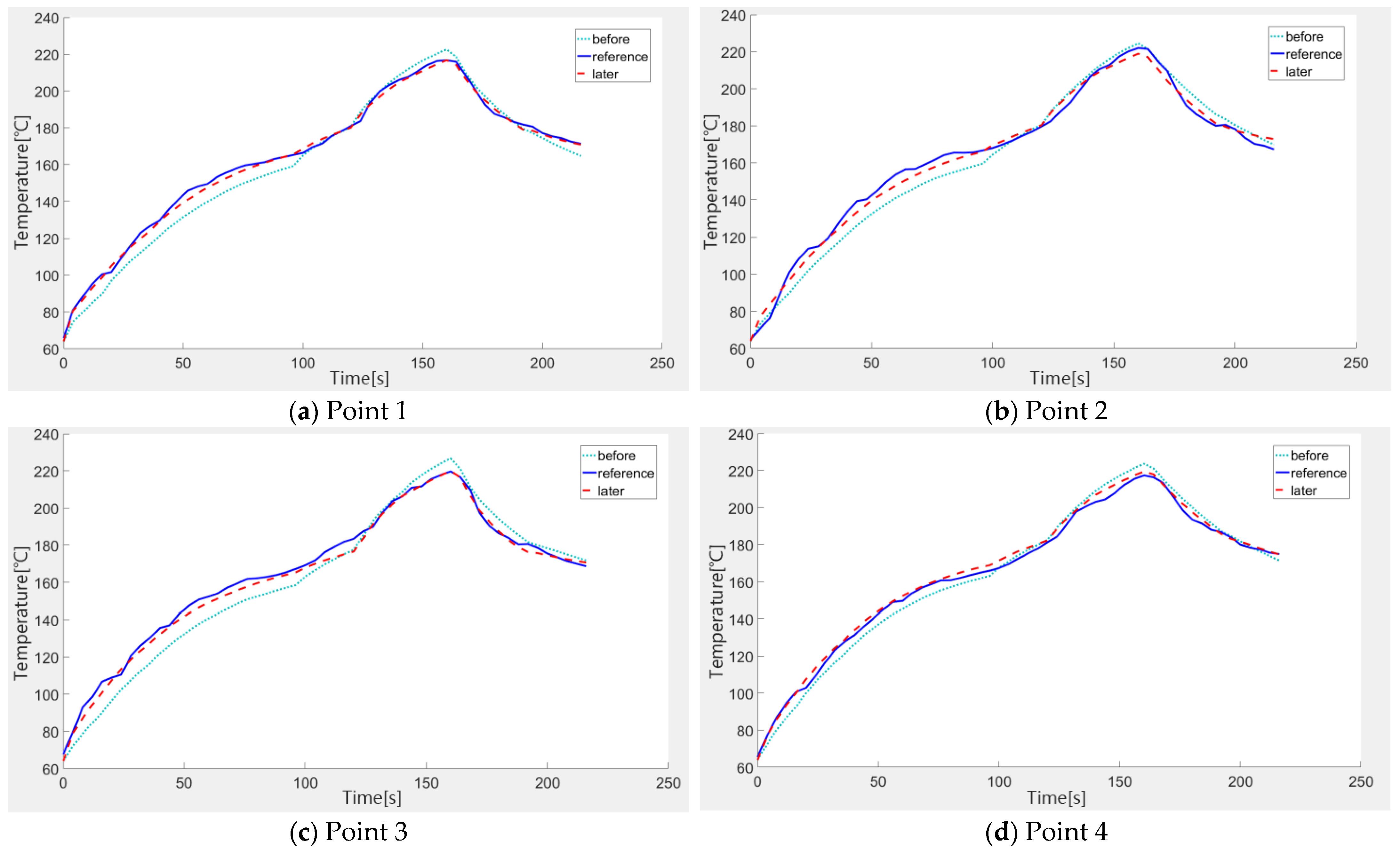
Point	Before Correction			After Correction
	Maximum Temperature Deviation * Δ/°C	Δ ≥ 10 °C/%	Δ ≥ 5 °C/%	Maximum Temperature Deviation Δ/°C	Δ ≥ 10 °C/%	Δ ≥ 5 °C/%
1	12.63	27.1	50.9	4.80	0	0
2	12.95	27.3	54.6	6.47	0	15
3	16.79	31.0	70.9	6.87	0	9
4	8.18	0	40.0	5.34	0	1.8

* The temperature data in the table were taken at 4 s intervals, a total of 55 samples.

, respectively.

It can be seen from Figure 17 and Table 9 that the accuracy of the simulation model with corrected nozzle-matrix gas flow velocity is much higher than the accuracy of the original model. For the temperature profiles of the PCBA component of the simulation model with corrected nozzle-matrix gas flow velocity, the maximum deviation from the test data is within 10 °C, and for at least 85% of cases, the maximum deviation is less than 5 °C. Consequently, the accuracy can meet the requirements of the actual process design (the generally required deviation is within ± 10 °C).

5. Conclusions

A new calculation approach for the nozzle-matrix gas flow velocity during hot air convection reflow soldering process is proposed in this paper. The approach is based on the theoretical calculation result of the H. Martin formula, the CFD numerical simulation and the temperature test of the aluminum alloy thin plate during the reflow soldering process. The CFD temperature model of the aluminum alloy thin plate during reflow soldering process is conducted and the temperature profiles are compared with those of the test. The temperature deviations between the model and the test for the thin plate is obtained and minimized by optimizing the nozzle-matrix gas flow velocity based on the reverse analysis. The temperature results using the corrected nozzle-matrix gas flow velocity in the CFD simulation are compared with the actual PCBA temperature test data. The results show that the maximum temperature deviation between the simulation and the test is less than 10 °C, and for most cases it is less than 5 °C. This proves that the nozzle-matrix gas flow velocity of the hot air reflow soldering process obtained by the new approach is accurate, and based on the new approach the temperature model of the PCBA during the soldering process is significantly improved.

References

- Lau, C.S.; Abdullah, M.Z.; Ani, F.C. Effect of solder joint arrangements on BGA lead-free reliability during cooling stage of reflow soldering process. IEEE Trans. Compon. Packag. Manuf. Technol. 2012, 2, 2098–2107. [Google Scholar] [CrossRef]
- Huang, B.Y.; Sun, G.Z.; Zhang, T.L. Mathematics model of reflow soldering temperature field in SMT. Electron. Process Technol. 2005, 26, 333–335. [Google Scholar]
- Gong, Y. Study on Optimization of Furnace Temperature Profile Under Reflow Soldering. Hot Work. Technol. 2013, 45, 187–190. [Google Scholar]
- Esfandyari, A.; Bachy, B.; Raithel, S.; Syed-Khaja, A.; Franke, J. Simulation, optimization and experimental verification of the over–pressure reflow soldering process. Procedia CIRP 2017, 62, 565–570. [Google Scholar] [CrossRef]
- Ngo, T.T.; Go, J.; Zhou, T.; Nguyen, H.V.; Lee, G.S. Enhancement of exit flow uniformity by modifying the shape of a gas torch to obtain a uniform temperature distribution on a steel plate during preheating. Appl. Sci. 2018, 8, 2197. [Google Scholar] [CrossRef]
- Ngo, T.T.; Zhou, T.; Go, J.; Nguyen, H.V.; Lee, G.S. Improvement of the steel-plate temperature during preheating by using guide vanes to focus the flame at the outlet of a gas torch. Energies 2019, 12, 869. [Google Scholar] [CrossRef]
- Lau, C.S.; Abdullah, M.Z.; Khor, C.Y. Optimization of the reflow soldering process with multiple quality characteristics in ball grid array packaging by using the grey-based Taguchi method. Microelectron. Int. 2013, 30, 151–168. [Google Scholar] [CrossRef]
- Abas, A.; Ishak, M.H.H.; Abdullah, M.Z.; Khor, S.F. Lattice Boltzmann method study of bga bump arrangements on void formation. Microelectron. Reliab. 2016, 56, 170–181. [Google Scholar] [CrossRef]
- Haslinda, M.S.; Abas, A.; Ani, F.C.; Jalar, A.; Saad, A.A.; Abdullah, M.Z. Discrete phase method particle simulation of ultra-fine package assembly with SAC305-TiO2 nano-reinforced lead free solder at different weighted percentages. Microelectron. Reliab. 2017, 79, 336–351. [Google Scholar] [CrossRef]
- Sahrudin, I.N.; Aziz, M.S.A.; Abdullah, M.Z.; Salleh, M.A.A.M. Molecular dynamics simulation of the nano-reinforced lead-free solder at different reflow soldering process temperature. IOP Conf. Ser. Mater. Sci. Eng. 2019, 701, 012014. [Google Scholar] [CrossRef]
- David, C.W.; Stuart, M.H. A simplified model of the reflow soldering process. Solder. Surf. Mount Technol. 2002, 14, 30–37. [Google Scholar]
- Gong, Y.; Li, Q.; Yang, D.G. The optimization of reflow soldering temperature profile based on simulation. In Proceedings of the IEEE 7th International Conference on Electronic Packaging Technology, Shanghai, China, 26–29 August 2006; pp. 1–4. [Google Scholar]
- Srivalli, C.; Abdullah, M.Z.; Khor, C.Y. Numerical investigations on the effects of different cooling periods in reflow-soldering process. Heat Mass Transfer 2015, 51, 1413–1423. [Google Scholar] [CrossRef]
- Iqbal, A.M.; Aziz, M.S.A.; Abdullah, M.Z.; Ishak, M.H.H. Temperature prediction on flexible printed circuit board in reflow oven soldering for motherboard application. IOP Conf. Ser. Mater. Sci. Eng. 2019, 530, 012019. [Google Scholar] [CrossRef]
- Lai, Y.; Park, S. Reflow profiling with the aid of machine learning models. Solder. Surf. Mt. Technol. 2023. ahead-of-print. [Google Scholar] [CrossRef]
- Lai, Y.; Ha, J.H.; Deo, K.A.; Yang, J.; Yin, P.; Park, S. Reflow Recipe Establishment Based on CFD-Informed Machine Learning Model. IEEE Trans. Compon. Packag. Manuf. Technol. 2023, 13, 127–134. [Google Scholar] [CrossRef]
- Deng, S.S.; Hwang, S.J.; Lee, H.H. Temperature prediction for system in package assembly during the reflow soldering process. Int. J. Heat Mass Transfer 2016, 98, 1–9. [Google Scholar] [CrossRef]
- Illés, B.; Bakó, I. Numerical study of the gas flow velocity space in convection reflow oven. Int. J. Heat Mass Transfer 2014, 70, 185–191. [Google Scholar] [CrossRef]
- Steenberge, N.V.; Limaye, P.; Willems, G.; Vandevelde, B.; Schildermans, I. Analytical and finite element models of the thermal behavior for lead-free soldering processes in electronic assembly. Microelectron. Reliab. 2007, 47, 215–222. [Google Scholar] [CrossRef]
- Martin, H. Heat and mass transfer between impinging gas jets and solid surfaces. Adv. Heat Transf. 1977, 13, 1–60. [Google Scholar]
- Chen, X.; Liu, H.; Wei, L.I. Experimental Investigation of Multiply Intensive Circular Air Impingement Jets Heat Transfer. Ind. Furn. 2016, 38, 19–23. [Google Scholar]
- Most, T.; Will, J. Metamodel of Optimal Prognosis-an automatic approach for variable reduction and optimal metamodel selection. Proc. Weimar. Optim.-Und Stochastiktage 2008, 5, 20–21. [Google Scholar]
- Roos, D.; Most, T.; Unger, J.F.; Will, J. Advanced surrogate models within the robustness evaluation. Proc. Weimar. Optim.-Und Stochastiktage 2007, 4, 29–30. [Google Scholar]
- Liu, X.; Zhou, D. Research on modeling and simulation of PCBA reflow soldering process based on the ICEPAK. Aviat. Precis. Manuf. Technol. 2013, 49, 25–29. [Google Scholar]
- Pistone, G.; Vicario, G. Kriging prediction from a circular grid: Application to wafer diffusion. Appl. Stoch. Models Bus. Ind. 2013, 29, 350–361. [Google Scholar] [CrossRef]