Fuzzy-Based Active Queue Management Using Precise Fuzzy Modeling and Genetic Algorithm

Abstract

Active Queue Management (AQM) methods significantly impact the network performance, as they manage the router queue and facilitate the traffic flow through the network. This paper presents a novel fuzzy-based AQM method developed with a computationally efficient precise fuzzy modeling optimized using the Genetic Algorithm. The proposed method focuses on the concept of symmetry as a means to achieve a more balanced and equitable distribution of the resources and avoid bandwidth wasting resulting from unnecessary packet dropping. The proposed method calculates the dropping probability of each packet using a precise fuzzy model that was created and tuned in advance and based on the previous dropping probability value and the queue length. The tuning process is implemented as an optimization problem formulated for the b₀, b₁, and b₂ variables of the precise rules with an objective function that maximizes the performance results in terms of loss, dropping, and delay. To prove the efficiency of the developed method, the simulation was not limited to the common Bernoulli process simulation; instead, the Markov-modulated Bernoulli process was used to mimic the burstiness nature of the traffic. The simulation is conducted on a machine operated with 64-bit Windows 10 with an Intel Core i7 2.0 GHz processor and 16 GB of RAM. The simulation used Java programming language in Apache NetBeans Integrated Development Environment (IDE) 11.2. The results showed that the proposed method outperformed the existing methods in terms of computational complexity, packet loss, dropping, and delay. As such, in low congested networks, the proposed method maintained no packet loss and dropped 22% of the packets with an average delay of 7.57, compared to the best method, LRED, which dropped 21% of the packets with a delay of 10.74, and FCRED, which dropped 21% of the packets with a delay of 16.54. In highly congested networks, the proposed method also maintained no packet loss and dropped 48% of the packets, with an average delay of 16.23, compared to the best method LRED, which dropped 47% of the packets with a delay of 28.04, and FCRED, which dropped 46% of the packets with a delay of 40.23.

1. Introduction

The ever-growing sharing of large multimedia files, using the Internet-of-Things (IoT) and the growth of applications and device controls remotely increase computer network utilization and distribution [1]. The communication between the distributed devices and applications is intermediated with router devices, which are responsible for transferring all transmitted packets via the network while maintaining the network performance [2]. The challenge these routers face is embodied in the number of transmitted packets that may exceed their capacity. Congestion occurs as the router’s buffer is overflowed, and no more packets can be accommodated. In such a case, packet loss occurs, and the network’s performance is dropped significantly [3,4]. Active Queue Management (AQM) methods control the queue at the router buffer and avoid congestion. The packets that arrive at the router are accommodated in the buffer as long as possible while packet loss occurs otherwise. Packet dropping is implemented as the expected situation exposes the overloading or overflowing of the router buffer. If packet dropping is not implemented efficiently, packet loss will be presented as packets cannot be accommodated. For its role in actively managing the queue at the router buffer, various AQM methods were proposed to replace the old method for queue management, the Drop-Tail (DT). The existing AQM methods are built on two main components: (1) network status variables and (2) dropping schemes [5].

The AQM’s status variables perceive the buffer and the traffic for efficiently operating the packet-dropping scheme. These variables are updated with every networking event to observe the traffic. Various variables have been used in the literature, such as the average queue length (AQL), the queue length (Q), and the change in the queue (ΔQ). The first AQM, random early detection (RED) [6], relied on the AQL variable, which showed limitations in response to sudden congestion as value changing is very slow. The Q variable is more efficient in addressing such congestion status yet leads to increased packet dropping in short-term high traffic status (i.e., false congestion). Generally, selecting the status variable depends on the expected network behavior (i.e., congested vs. low-traffic network). Unfortunately, no standard network status variable is to be used, and no specific network behavior can be expected. Thus, no mechanism exists to identify the most appropriate status variables [7].

The stochastic packet-dropping scheme of the AQM considers the status of the network. In highly congested networks, dropping is increased to prevent loss, as loss leads to bad consequences with packet retransmission. As the flow reduces, dropping should be stopped as packet dropping leads to delays, increases traffic, and consumes more resources. The dropping scheme also considers the problem of global synchronization to maintain high network performance in different states [8]. The dropping action is performed by calculating a dropping probability, which is translated into stochastic packet dropping. The problem with the decision-making techniques utilized in the AQM methods is that they are manually created, which shows limitations in addressing the expected burstiness of the network traffic [9].

The early AQM methods calculate the value of the dropping probability (Dp) based on the value of the status variables using a set of rules wrapped in case-based reasoning; these methods can be denoted as crisp-based AQM methods. These methods were extended with the fuzzy inference process to ease the parameterization problem and reduce packet loss [10]. For the fuzzy-based methods, the fuzzy system is formed using input variables mapped from the status variables in the crisp-based AQM methods while the output variable represents the Dp. The fuzzy rules are equivalent to the decision rules in the crisp-based methods. Although the results of fuzzy-based methods are better than those of crisp-based methods, there are limitations to these methods related to the performance of the network and the computation requirements. Moreover, fuzzy-based methods showed a high drop rate, especially when encountering low traffic [11]. The reasons for such results are as follows: (1) using the same variables as those utilized in the crisp-based methods but using different techniques and (2) using a non-adaptive process that implements unnecessary high or low dropping with loss. (3) The linguistic technique of fuzzy systems is not precise in forming the problem based on the given inputs. (4) Using expert-constructed and tuned rules does not produce the optimal results, similar to the rules in the crisp-based methods.

In summary, the fuzzy-based AQM methods extend the crisp methods using fuzzy logic systems. The existing fuzzy-based AQM methods are built using the linguistic model using rules constructed by experts in the domain. The results of these fuzzy AQM methods are better than the crisp-based methods in parameterization and packet loss. However, the fuzzy AQM methods suffer from a high dropping rate and computation requirements. Moreover, the dropping problem of these methods indicates the low adaptiveness of these AQM methods, which harms the network performance with the bursty nature of the traffic. This paper proposes a novel fuzzy-based AQM to address the limitations of the existing fuzzy-based AQM and improve the network’s performance. The proposed method focuses on the concept of symmetry as a means to achieve a more balanced and equitable distribution of the resources and avoid bandwidth wasting resulted from unnecessary packet dropping. The proposed method is developed based on inputs that do not require a mapping from crisp-based AQM and uses a computationally efficient fuzzy approach. The proposed method uses a simple variable and precise fuzzy model instead of a linguistic one. First, the input variables are identified. Then, the fuzzification rules are constructed in their generic forms. The rules are then tuned using the Genetic Algorithm (GA) to overcome the limitations of the human-generated rules. The constructed system is then used to calculate the Dp value based on the Q value only. In the simulation process, both the Bernoulli and the Markov modulated Bernoulli are used to mimic the traffic’s burstiness and evaluate the proposed method effectively. The rest of this paper is organized as follows: Section 2 presents a literature review on the crisp-based and fuzzy-based AQM methods with a brief overview of the existing fuzzy inference processes and systems. The proposed work includes the proposed framework, the utilized variables, rules, and the algorithm, which are discussed in Section 3. The simulation settings and the results are presented in Section 4. Finally, Section 5 presents the conclusion of this paper.

2. The Literature Review

The AQM is founded on a decision-making approach that comprises multiple rules designed to determine appropriate actions based on the network and buffer status. Within the AQM, these decision rules function as mappings, translating observed values of status variables into suitable actions related to dropping packets. The typical decision-making steps within the AQM process are illustrated in Figure 1 [12]. Existing AQM methods are broadly categorized into two main types: crisp-based AQM and fuzzy-based AQM. Fuzzy-based methods expand upon the crisp approach by incorporating the fuzzy inference process, as illustrated in Figure 2 [10].

2.1. The Crisp-Based AQM Methods

AQM methods depend on tracking some status variables and managing the queue at the router buffer using a packet-dropping mechanism. RED [6] is implemented based on the AQL status variable, the initial dropping probability (D_ini) parameter, and two manually predetermined thresholds. The AQL indicates the number of queued packets over time and guides the dropping process. The thresholds set different ranges with different consequences. As such, if the AQL is below the first threshold (i.e., the minimum threshold), the dropping probability is set to zero; as in such a case, the network is considered to be at a low load. If the calculated AQL is between the first and second threshold (i.e., the maximum threshold), stochastic dropping is implemented to avoid congestion as the flow is considered high. Finally, if the calculated AQL is higher than the second threshold, the dropping probability is set to one in such a case, as the network flow is considered aggressive. Figure 3 illustrates the status variable and the dropping mechanism implemented in RED [13].

Various crisp-based methods were proposed using different variables and mechanisms compared to the one implemented by the RED. Gentle RED (GRED) [14] is also based on the AQL and three thresholds instead of two. As such, if the AQL is below the first threshold or higher than the third threshold, the dropping probability is set to zero and one, respectively, similar to RED. However, compared to RED, GRED had more flexibility in calculating Dp when the AQL is between the first and second thresholds or between the second and third thresholds. Accordingly, GRED is more responsive and fixable but requires more parameter settings. The Adaptive RED (ARED) [15] is also based on the AQL, two thresholds, and one target variable. Moreover, the D_ini value is changed adaptively based on the value of the AQL. If the AQL is below the first threshold or higher than the third one, the dropping probability is set to zero and one, respectively, similar to RED and GRED. Dp is calculated such that the AQL value shall be close to the target value when the AQL is between the first and second thresholds. Overall, ARED is similar to GRED in responsiveness and flexibility and is more adaptive than GRED and RED. RED, GRED, and ARED used the same status variables and variations of the dropping scheme. Effective RED (ERED) [16] used AQL and Q. Multi-level RED (MRED) [17] used packet loss (PL), while the Adaptive Virtual Queue (AVQ) [18], Stabilized AVQ (SAVQ) [19], and Enhanced AVQ (EAVQ) [20] used the arrival rate. Link Utilization Based AQM (LUBA) [21], Stabilized Virtual Buffer (SVB) [22], Rate-Based AQM (RAQM) [23], Robust Active Queue (RaQ) [24], and Yellow [25] used load rate and arrival rate. Curvy Random Early Detection (CurvyRED) [26] and various other techniques [27,28] use the delay as a status variable.

Various adaptive strategies were put forth during the AQM’s evolution. The term “adaptive” has been used in two ways: (1) to calculate the values of the utilized variables that are being used rather than using fixed values, and (2) to increase or decrease the value of a variable rather than recalculating it or using a fixed value. Many methods, including RED, rely on initialized variables that might negatively affect performance; these variables are modified to be adaptive as implemented by ARED and New Adaptive RED (NARED) [29]. Accordingly, in such a case, adaptive techniques minimize the number of parameter sittings required and improve the response time to congestion. ARED, NARED, and Adaptive Threshold RED [30] used adaptive values for the variable D_ini while Length-Threshold RED (LTRED) [31] and Probability-RED (P-RED) [32] modified the value of the AQL adaptively. The second direction of the adaptive technique involves increasing and decreasing the value of a variable based on its previous value. BLUE [33] calculated the value of Dp adaptively. BLUE used a mechanism that adaptively increases and decreases the Dp value with reference to loss and buffer utilization. In such a case, the congestion responsiveness was improved, and the performance was stabilized as the value of Dp was stabilized. Linear RED (LRED) [34] developed a linear equation with calculations to reduce the complexity of RED. Integrated RED (IRED) [35] used arrival, departure, and queue length factors to improve the AQM performance.

Table 1. Summary of the Crisp-Based AQM Methods.

Method	Title	Control Variable(s)	Aims
RED	Random Early Detection	AQL	Eliminate global synchronization and improve packet loss
GRED	Gentle RED	AQL	Improve packet loss
ARED	Adaptive RED	AQL	Improve packet loss
MRED	Multi-level RED	PL	Improve packet loss
AVQ	Adaptive Virtual Queue	Arrival	Improve packet delay
SAVQ	Stable AVQ	Arrival	Improve packet delay
EAVQ	Enhanced AVQ	Arrival	Improve packet delay
ERED	Effective RED	AQL and Q	Improve packet loss
LUBA	Link Utilization-Based AQM	Load	Improve packet delay
SVB	Stabilized Virtual Buffer	Arrival and Q	Improve packet loss and resource utilization
RAQM	Rate-Based AQM	Arrival and Q	Improve packet loss and resource utilization
RaQ	Robust Active Queue	Arrival and Q	Improve resource utilization
Yellow	N/A	Arrival and Q	Improve resource utilization
CurvyRED	N/A	Delay	Improve packet delay
NARED	New Adaptive RED	AQL	Ease parameter initialization
ATRED	Adaptive Threshold RED	AQL	Ease parameter initialization
LTRED	Length-Threshold RED	AQL	Ease parameter initialization
P-RED	Probability-RED	AQL	Ease parameter initialization
BLUE	N/A	PL	Improve packet loss
Delay-based	N/A	Delay	Improve delay
LRED	Linear RED	AQL	Reduce the complexity
IRED	Integrated RED	Arrival, Departure, and Q	Improve the performance

summarizes the existing work on crisp-based AQM methods.

2.2. The Fuzzy-Based AQM Methods

Fuzzy-based AQM methods use the network status variables in the crisp-based methods with a fuzzy system. The ranges of the values for the input and output variables are initiated based on predefined membership functions. The rules of the fuzzy system create more variations in the decision-making processes compared to the limited decisions created in the crisp-based AQM. The fuzzy-based AQM methods have been implemented using different inputs, membership functions, rule-sets, and a slight variation of the output variable. The Fuzzy RED [36] method used Q and ∆Q as equivalent to AQL in the RED method, and the Fuzzy Explicit Marking (FEM) [37] used the same input variables with different processes. Fuzzy BLUE (FBLUE) [38] used buffer size and packet loss as input variables, Fuzzy GREEN [39] used Q and dropping rate, Fuzzy-logic Controller-based RED [40] used AQL and Pl, and Fuzzy-logic RED (FLRED) [41] used the delay and AQL as the input variables. Fuzzy Comprehensive RED (FCRED) [42] used three indicators, which monitor the router’s arrival, departure, and queue length.

Table 2. Summary of the Fuzzy-Based AQM Methods.

Method	Title	Control Variable(s)	Aims
Fuzzy RED	Fuzzy RED	Q and ∆Q	Ease the parameter initialization
FEM	Fuzzy Explicit Marking	Q and ∆Q	Ease the parameter initialization
FBLUE	Fuzzy BLUE	Loss and Q	Ease the initialization and adaptively calculating Dp
Fuzzy GREEN	Fuzzy GREEN	Dropping and Q	Ease the parameter initialization
Fuzzy-Controller-RED	Fuzzy Controller RED	AQL and loss	Ease the parameter initialization
FYZREM	Fuzzy REM	Packet price	Ease the parameter initialization
Deep-BLUE	Deep BLUE	Loss and Q	Ease the initialization and adaptively calculating Dp
Fuzzy-ARED	Fuzzy ARED	AQL	Ease the parameter initialization
FGRED	Fuzzy GRED	AQL and Delay	Ease the initialization
FLRED	Fuzzy Logic RED	AQL and delay	Ease the initialization and Improve packet dropping
FCRED	Fuzzy Comprehensive RED	Load and Q	Improve packet dropping

summarizes the existing work on fuzzy-based AQM methods. These fuzzy-based AQM methods used the linguistic modeling approach proposed by Mamdani [43].

2.3. Fuzzy System Models

There are two approaches to modeling the fuzzy system: the linguistic and precise models [44]. The linguistic modeling approach is characterized by its interpretability with a low ability to model the system precisely (i.e., accuracy). Takagi and Sugeno proposed the precise modeling approach, commonly called the TSK fuzzy system. The precise model is characterized by its low interpretability and high accuracy. The difference between linguistic and precise modeling is implied in the rule set, which consists of linguistic variables only in the linguistic approach. Thus, a defuzzification component is required to convert the output linguistic variable into a crisp value. The precise modeling uses a rule set of linguistic and crisp variables and does not require a defuzzification component. Figure 4 illustrates the linguistic and precise models for fuzzy systems, and

Table 3. Linguistic vs. Precise Fuzzy Models Comparison.

Comparison Criteria	Linguistic (Mamdani)	Precise (TSK)
Membership Function	Input and Output	Input only
Defuzzification	Required	Not required
The Output of Surface	Discontinuous	Continuous
Developing Complexity	Simple	Complex
Understanding Complexity	Intuitive (Human-Interpretation)	Complex (Mathematical-Interpretation)
System Design	Rigged	Flexible

compares the two models [45].

Although these models have great differences, they have similar components of input, membership function, and rule set [46,47]. Identifying the rule set is the most complex task in building the fuzzy system [48]. The rule set can be constructed using one of two approaches: knowledge-based and data-based. The knowledge-based required human experts to construct the rules. The problem with this approach is the limitation of the constructed knowledge base. The data-driven approach learns the rule set from sample data [49]. While a data-driven approach is more adequate in covering all the detailed mapping between inputs and outputs, the rules lose merit if a purely data-driven approach is utilized. A comparison between the knowledge-based and the data-driven approaches is given in

Table 4. Knowledge-based vs. Data-Driven Rule Construction.

Comparison Criteria	Knowledge-Based	Data-Driven
Generality and Adequacy	Not granted	Granted
Rule Preciseness	Granted	Suspicious
Rule Complexity	Interpretable	Ambiguous
Rule Transparency	Yes	No (Questionable)

[50].

While the existing AQM methods use the linguistic approach, the precise approach may produce more accurate results. An advantage of some crisp-based methods is their adaptiveness, which is too complex to be modeled using the linguistic approach for fuzzy systems. Accordingly, an adaptive method can be developed using a precise fuzzy approach. The resulting system’s complexity can be eased using an optimization technique to tune the rule set and produce the desired output.

3. The Proposed Work

The proposed Fuzzy Random Early Detection with GA (FREDGA) method used the queue length, Q, a simple counter for the number of packets residing in the queue, in an adaptive mechanism. The variable Q did not require any calculation or parameter settings, such as those required in calculating the AQL. Accordingly, using Q was more efficient compared to using AQL. The drawback of using Q was overcome as the proposed method adaptively calculated a new Dp value based on the previously calculated Dp. A computationally efficient and precise fuzzy-logic system was built, tuned using GA, and used.

3.1. The Framework

The following steps were used to operate the proposed method and calculate the value of Dp with each packet arrival. (1) The Q’s value was updated. (2) The pre-built fuzzy model was executed. Fuzzification, rule evaluation, and aggregation were all carried out accordingly. (3) The decision-making process was applied, and the decision to drop or accommodate was made. The rules were constructed and tuned before the previously mentioned arrival-based processes. The rules were constructed and tuned using a solution-optimization process that identified the best rules using GA. Figure 5 shows the flowchart of the proposed framework.

3.2. The Fuzzy Set and Function

The proposed method used two input variables for the fuzzy logic system: the queue length, Q, and the previously calculated Dp. These two crisp variables are simple because Q does not need any calculation while Dp is the output of the fuzzy system. Initially, both values were set to zero as the system was initiated, and then, the Q value was updated based on packet arrival and departure. The value range for the Q was [0–capacity], and the value range for the Dp was [0–1]. To unify the range of these two variables, the value of Q was divided by the capacity, and the results would be in the range of [0–1], as given in Equation (1).

$$Q_{nor}=Q/capacity, \in [0-1]$$

(1)

where Q_nor was the normalized Q value and will be referred to as Q for the rest of this paper, Q was the original queue length, and the capacity was the buffer size.

The crisp inputs were converted into linguistic terms using the membership functions and the fuzzy sets. One of the two approaches mentioned earlier (i.e., knowledge-based and data-based) was used to construct these two fuzzy components. The membership function and set definitions were related to constructing the rule set. However, the membership function and sets were identified separately to ease the construction of the fuzzy system. Based on the space-partitioning approach for fuzzy system construction [51], the domain of each input was divided into equal-sized 2n + 1 regions (i.e., the value of n is set to equal to 1) that were used to form the function with three terms. As illustrated in Figure 6, the membership function was trapezoidal, and the boundaries of the function were set to [{0, 0, 0.3, 0.4}, {0.3, 0.4, 0.6, 0.7}, {0.6, 0.7, 1.0, 1.0}], with low, moderate, and high terms.

3.3. The Fuzzification Process

As a packet arrival occurred, the Q value was updated and used as an input to the fuzzy system with the previously calculated Dp. Accordingly, at a time t, the input of the fuzzy system was Q_t (after normalization as given in Equation (1)) and Dp_t−1. The crisp values for Q_t and Dp_t−1 were converted into linguistic terms with confidence degrees in the fuzzification processes. The fuzzification of a single value may produce more than a single term, each with a confidence value. Each variable needed a linguistic set and a membership function, as discussed in the previous subsection. The regions of the membership function were identified by 2–3 lines and four points, a₁, b₁, a₂, and b₂, where a and b are the upper and lower bounds of the horizontal lines of each region.

Using Equation (2), each crisp value was converted to a confidence degree associated with a specific term. At least a linguistic term from the linguistic set was identified for each crisp input. Equation (2) was applied for the input of three terms set to produce three confidence values, each for a single term. Terms with zero confidence were removed.

$$\mathcal{d}\left(v\right)=\left\{\begin{array}{cc}\begin{array}{c}0,\\ v-a_1/b_1-a_1,\\ \begin{array}{c}1,\\ b_2-v/b_2-b_1,\end{array}\end{array}& \begin{array}{c}if v<a_1, v>b_2\\ if a_1\le v\le b_1\\ \begin{array}{c}if b_1\le v\le a_2\\ if a_2\le v\le b_2\end{array}\end{array}\end{array}\right.$$

(2)

where d(v) was the confidence degree for the input value v while a₁, b₁, a₂, and b₂ were the boundary points for each linguistic term in the membership function.

3.4. The Rule Set Construction and Utilization

The proposed method was created using the TSK model, as opposed to the existing AQM methods, which used the fuzzy linguistic model. Each rule in the proposed method connected inputs to an output value, such as linguistic terms with confidence values representing the inputs, while the output was represented as a crisp value (while in the linguistic model, the output was also represented as a linguistic term). As given in Equation (3), each rule comprised a combination of different inputs. The set of N rules covered all possible combinations of the input values (i.e., 9 (3 × 3) different rules for the proposed method). Each rule formed a mapping function f, which mapped the values of the inputs into dropping probability y, as given in Equation (4).

$${Rule}^1:\left({x_1}^{\left(1\right)},{x_2}^{\left(1\right)};y^{\left(1\right)}\right),{Rule}^2\left({x_1}^{\left(2\right)},{x_2}^{\left(2\right)};y^{\left(2\right)}\right),\dots ,{Rule}^N({x_1}^{\left(N\right)},{x_2}^{\left(N\right)};y^{\left(N\right)})$$

(3)

$$f(x_1,x_2)\to y$$

(4)

where x₁ was a linguistic term for Q, x₂ was a linguistic term for Dp, and y was the output.

The output value y was calculated as given in Equation (5), which took the form of a first-order polynomial rather than a tangible value. Thus, the constructed rules were formed as a first-order TSK system. Accordingly, the concrete form of the constructed rules was given in Equation (6).

$$y=b_0+b_1{x}_1+b_2{x}_2$$

(5)

$$IF\mathrm{Q}=={\mathrm{X}}_1 \mathrm{a}\mathrm{n}\mathrm{d} {Dp}_{\mathrm{t}-1}=={\mathrm{X}}_2 \mathrm{T}\mathrm{H}\mathrm{E}\mathrm{N} y=b_0+b_1{x}_1+b_2{x}_2$$

(6)

where X₁ was a term value for Q, X₂ was a term value for Dp, and x₁, and x₂ were confidence values of the linguistic terms X₁ and X₂ while b₀, b₁, and b₂ were selected parameters that influenced the performance of the constructed system.

Based on the linguistic sets of the input variables, nine rules were constructed, but the values for the parameters b₀, b₁, and b₂ were assigned in the next step. These rules are listed in

Table 5. List of Cases for the Rule Construction Process.

#	Term 1 (Q)	Term 2 (Dp)	#	Term 1 (Q)	Term 2 (Dp)
1	low	low	6	moderate	high
2	low	moderate	7	high	low
3	low	high	8	high	moderate
4	moderate	low	9	high	high
5	moderate	moderate

, and Equation (7) provides a specific illustration of rule #2 from that table.

$$IF\mathrm{Q}==\mathrm{l}\mathrm{o}\mathrm{w} \mathrm{a}\mathrm{n}\mathrm{d} {Dp}_{\mathrm{t}-1}== \mathrm{m}\mathrm{o}\mathrm{d}\mathrm{e}\mathrm{r}\mathrm{a}\mathrm{t}\mathrm{e} \mathrm{T}\mathrm{H}\mathrm{E}\mathrm{N} {Dp}_{\mathrm{t}}=b_0+b_1{c}_{vLow}+b_2{c}_{moderate}$$

(7)

where c_Low and c_moderate were the confidence values of low and moderate linguistic terms of Q and Dp variables, respectively. The parameters b₀, b₁, and b₂ were constants in the range [0–1], which would be assigned values in the tuning process. The proposed method implemented a simple aggregation step that depended on averaging for the output of different applied rules.

3.5. The Rule Set Tuning

After creating the rules, they were tuned by finding the optimal values for the parameters b₀, b₁, and b₂, as illustrated in Figure 7. GA was selected for the tuning processes over many existing optimization algorithms because it is simple, performs well in varied environments, and can search huge and uneven solution spaces, such as the one under investigation. GA was used to optimize the performance of the proposed AQM method, which depended on the value of Dp. Dp optimization, in turn, was a function of b₀, b₁, and b₂. Accordingly, the optimization function for the proposed method is given in Equation (8).

$${Dp}_i={{f(b}_0}_i, {b_1}_i,{b_2}_i)$$

(8)

where i was the rule’s index in the rule set as given in Table 5, each with specific values for b₀, b₁, and b₂.

As such, there were 27 parameters to be optimized using GA for the nine rules. The processes that the GA implemented are illustrated in Figure 8. GA consisted of an initialization step, which created the initial population of multiple individuals. Each individual (i.e., a chromosome) consisted of 27 genes. The initialization process was implemented based on randomly generated values. In the evaluation process, the fitness function, which measured the performance of the AQM method based on the current values of b₀, b₁, and b₂, was calculated. The selection was implemented to select chromosomes from the old population to form the offspring, after which the crossover and mutation were implemented on the selected individuals. The process continued until the stopping criteria were met [52].

Equation (9) provided the fitness function (also known as the objective function), which was derived based on the problem, and Equation (10) provided the associated hard constraint.

$$f\left(v\right)=\begin{array}{c}avgmax\\ j\end{array} {\sum }_{i=1}^N{w}_i\times {v_i}^j/{\sum }_{i=1}^N{w}_i$$

(9)

$${\sum }_{i=1}^N{w}_i=1, \forall {v_i}^j\in [0-1]$$

(10)

where N was the set of the performance measures to be optimized, which were determined to be the delay, packet loss, and dropping rate at specific traffic load conditions. The value v_i^j was obtained for the performance measure i at iteration j. The value w_i was the weight of the performance measure i.

The soft constraint in Equation (9) aimed to maximize the performance based on the weighted sum of the multi-objective function. Each performance measure had a value in the range of [0–1] to avoid bias. In the proposed method, all three measures were given equal weights of 0.33 to find the optimal solution that suited the burstiness nature of the network. The hard constraint in Equation (10) ensured that the sum of the weights given to all the performances equals 1.

The encoding scheme of the problem to be optimized consisted of real values for the optimized constants, as illustrated in Figure 9.

The GA parameter setting was defined as given in

Table 6. GA Parameters.

GA Parameter	Size/Value/Scheme
Population size	20
Generation size	100
Replacement Scheme	Replace the worst 60%
Chromosome Length	27
Selection Scheme	Rank-based roulette
Crossover probability	0.95
Mutation probability	0.05

. The first generation in GA was randomly initialized. The population size was 20, and the stopping criterion was based on a steady state for ten iterations with maximum fitness variations below a small threshold (i.e., 0.0001) or reaching the maximum number of iterations. The GA selection operation type was roulette-wheel. The replacement type and ratio were “replacement of the worst and 60% in a steady state manner”. The crossover rate was 0.95, and the mutation rate was 0.05.

4. Simulation and Results

The conducted simulation consists of three main components: departure process, environment, and arrival process, similar to the previous AQM simulations. The departure process is simulated as a geometric distribution controlled with a departure probability β, while the arrival is simulated using the Bernoulli process (BP) and the Markov-modulated Bernoulli process (MMBP).

4.1. Traffic Classes

The arrival process is simulated in two forms: the Bernoulli process (BP), which models a single traffic class, and the Markov-modulated Bernoulli process (MMBP), which captures traffic burstiness using multiple classes [53]. These stochastic processes, BP and MMBP, characterize sequences of binary events with success or failure options. In this context, the binary events represent the packet arrival event. The BP models an independent sequence of events, each with a specific probability of success. The number of successes for a given trial follows a binomial distribution. On the other hand, the MMBP extends the BP by incorporating principles from Markov chains to model probabilities with varying values based on the current state of the Markov chain. As a result, the success probability fluctuates based on the existing state of a hidden Markov chain.

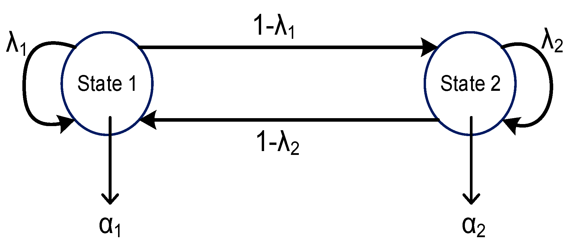
As such, BP represents a sequence of independent trials with a constant probability while the MMBP extends this concept by incorporating a Markov chain to model time-varying success probabilities. Both processes are valuable for modeling binary events in various scenarios, offering insights into the dynamics and characteristics of systems influenced by probabilistic outcomes. In the BP, the simulation utilizes an arrival probability, α, in a straightforward mechanism. The MMBP is modeled using a two-state model, as illustrated in Figure 10. The process starts with state 1 with an arrival probability of α₁. In the next time slot, the process remains in state 1 with a probability of λ₁ or is transmitted to state 2 with a probability of 1 − λ₁. On the other hand, if the current state is state 2, then the arrival probability is α₂. The process remains in state 2 in the next time slot with the probability of λ₂ or transmitted to state 1 with probability 1 − λ₂. Accordingly, the arrival process is characterized by the arrival diagonal matrix (R), and the transmission probability is characterized by the matrix T, as given in Equation (11).

$$\mathrm{R}=\left[\begin{array}{cc}{\mathsf{\alpha }}_1& 0\\ 0& {\mathsf{\alpha }}_2\end{array}\right],\mathrm{T}=\left[\begin{array}{cc}{\mathsf{\lambda }}_1& {1-\mathsf{\lambda }}_1\\ {1-\mathsf{\lambda }}_2& {\mathsf{\lambda }}_2\end{array}\right]$$

(11)

where R is the arrival probability matrix for the MMBP of two states, and T is the transmission matrix for the MMBP states represented by R.

4.2. The Simulation Environment

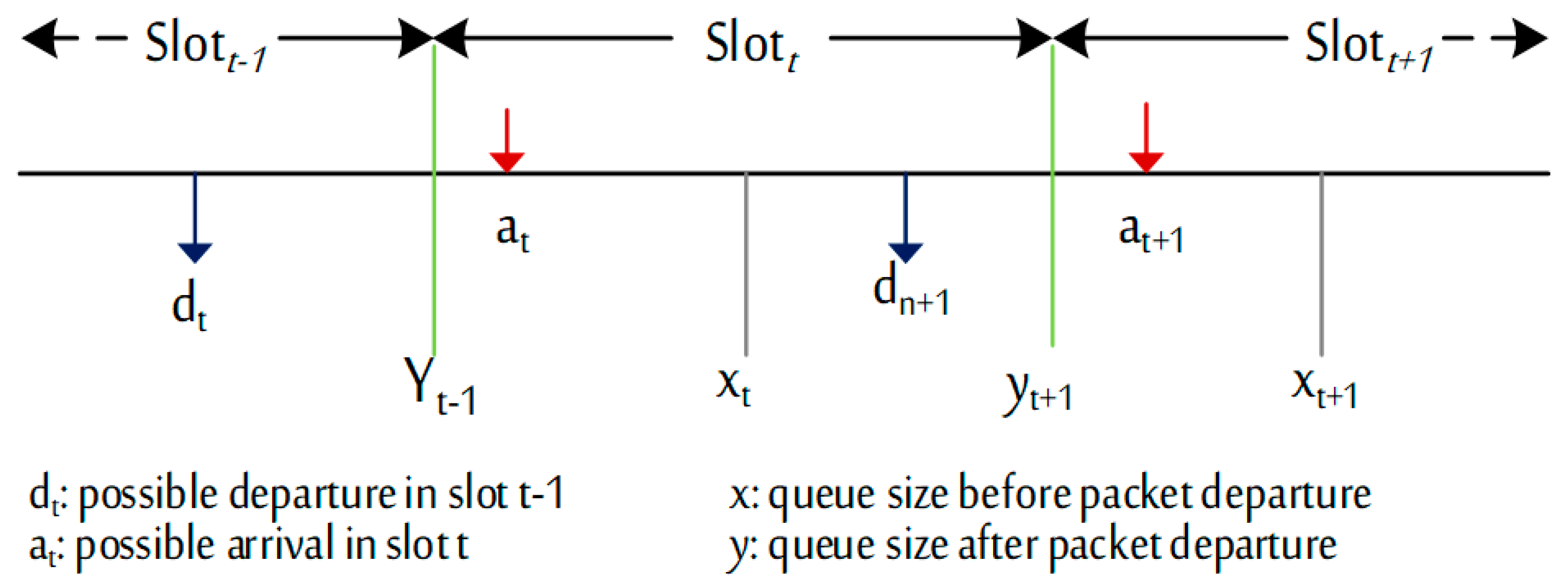
The simulation environment is the widely used discrete-time queue, which allows for evaluating the performance based on network events. The discrete-time queue model consists of time slots for unequal periods. A packet arrival and/or packet arrival occur in each slot. The departure event occurs before the arrival process, as illustrated in Figure 11. The simulated network events take place (stochastically) over a single router with a limited capacity buffer. The buffer is modeled using first in first out (FIFO) with a capacity of 20 packets, regardless of its type and size [54].

Using the discrete-time queue model in the conducted simulation provides a significant advantage by ensuring the reproducibility of the simulation process, regardless of the tools or programming language employed. This reproducibility is crucial as it guarantees consistent results that can be used to evaluate future methods, including real-world implementations. By adhering to this approach, simulation outcomes can serve as benchmarks for assessing novel techniques, enabling researchers and practitioners to make informed decisions based on reliable and consistent simulation results. However, it is important to recognize that the discrete-time queue model does have certain limitations, particularly when applied to real-world scenarios, such as computer networks. The primary limitation is related to the inherent simplifications and assumptions that the model entails. As such, the model might overlook external influences that significantly affect the network performance. Accordingly, the real-world implementation shall re-evolve the model using the GA and create a new rule set.

The simulation is conducted on a machine operated with 64-bit Windows 10 with an Intel Core i7 2.0 GHz processor and 16 GB of RAM. The simulation used Java programming language in Apache NetBeans Integrated Development Environment (IDE) 11.2. The simulation parameters are summarized in

Table 7. Parameter Settings.

Category	Parameter	Values
Simulation	Packet arrival probability in BP (α)	0.3–0.95
	Packet arrival probability in MMBP (α1 and α2)	0.3–0.95 and 0.5
	Probability of Packet Departure (β)	0.3 and 0.5
	Total Number of Slots	2,000,000
	Number of Slots for Warm-Up Period	800,000
	Number of Slots for the Results	1,200,000
	Capacity of the Router Buffer	20
Compared Methods	Queue Weight for AQL Calculation	0.002
	Dmax	0.1
	minth	3
	maxth	9

. Among the 2,000,000 slots implemented in the simulated environment, 800,000 are used as a warm-up period. The arrival probability α holds 14 values in the range [0.3–0.95] to create various congested and non-congested scenarios.

In evaluating the proposed method, the loss, drop, and delay are presented alongside the time required for the simulation. The results of the proposed method are compared to the well-known RED, ERED, and BLUE methods, together with the recently proposed LRED and IRED, which are crisp-based. In addition, the proposed method is also compared with early and recently developed fuzzy-based methods: Fuzzy RED (FRED), FGRED, FBLUE, and FCRED. Table 7 shows the compared methods’ parameters [55].

4.3. Optimization Results

GA is used to fine-tune the rules before running the experiments. The convolution of GA was remarkably quick, taking an average of only 100 iterations for 30 runs to reach the optimal solution. Figure 12 shows the results in one of these runs with 63 iterations, and the value obtained by the best solution is provided in Appendix A.

4.4. AQM Results

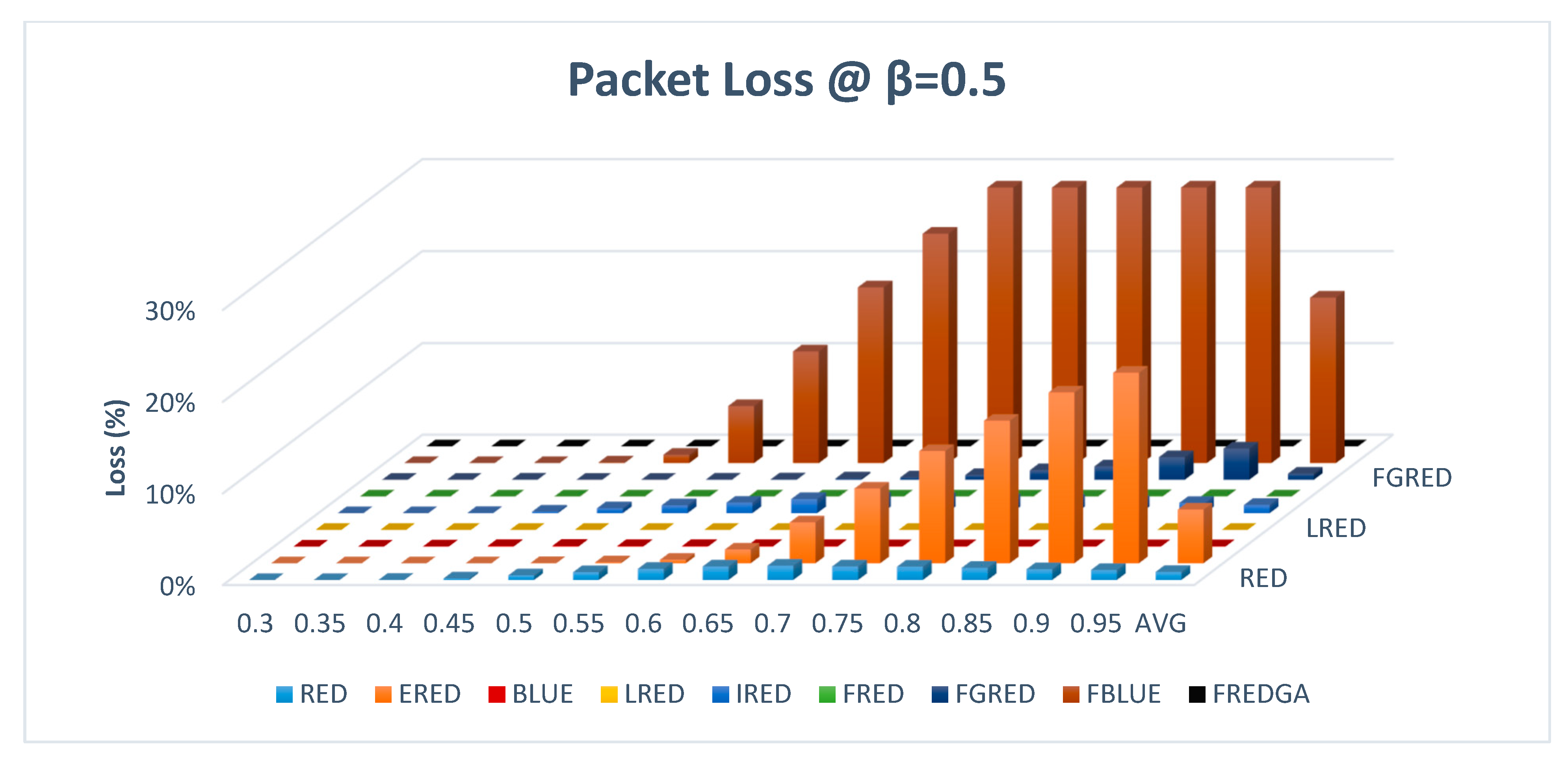
The proposed method is implemented and evaluated in two experiment sets with a single traffic class. The first experiment was conducted with a β value of 0.5 and all α values. The second experiment is conducted with a β value of 0.3. Figure 13 illustrates the evaluation based on loss, with β value of 0.5 and a single traffic class.

As results showed, the proposed FREDGA method lost no packets regardless of the arrival rate, similar to BLUE, LRED, FRED, and FCRED. FBLUE and ERED, on the other hand, had suffered significant losses of 18% and 6% of the total number of packets sent across the simulated network, respectively. An amount of 1% of the transmitted packets were lost using the RED, IRED, and FGRED methods.

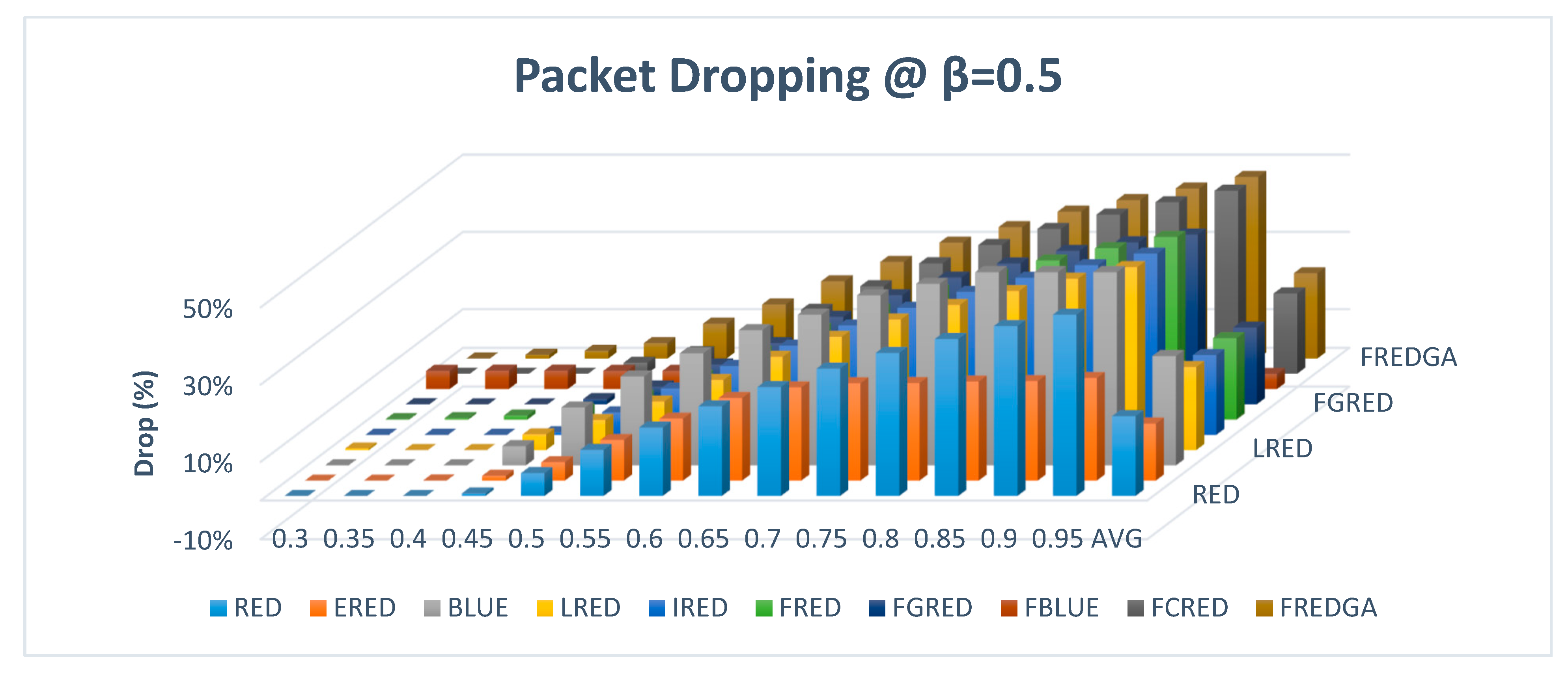
Figure 14 illustrates the evaluation results based on dropping with β value of 0.5 and a single traffic class.

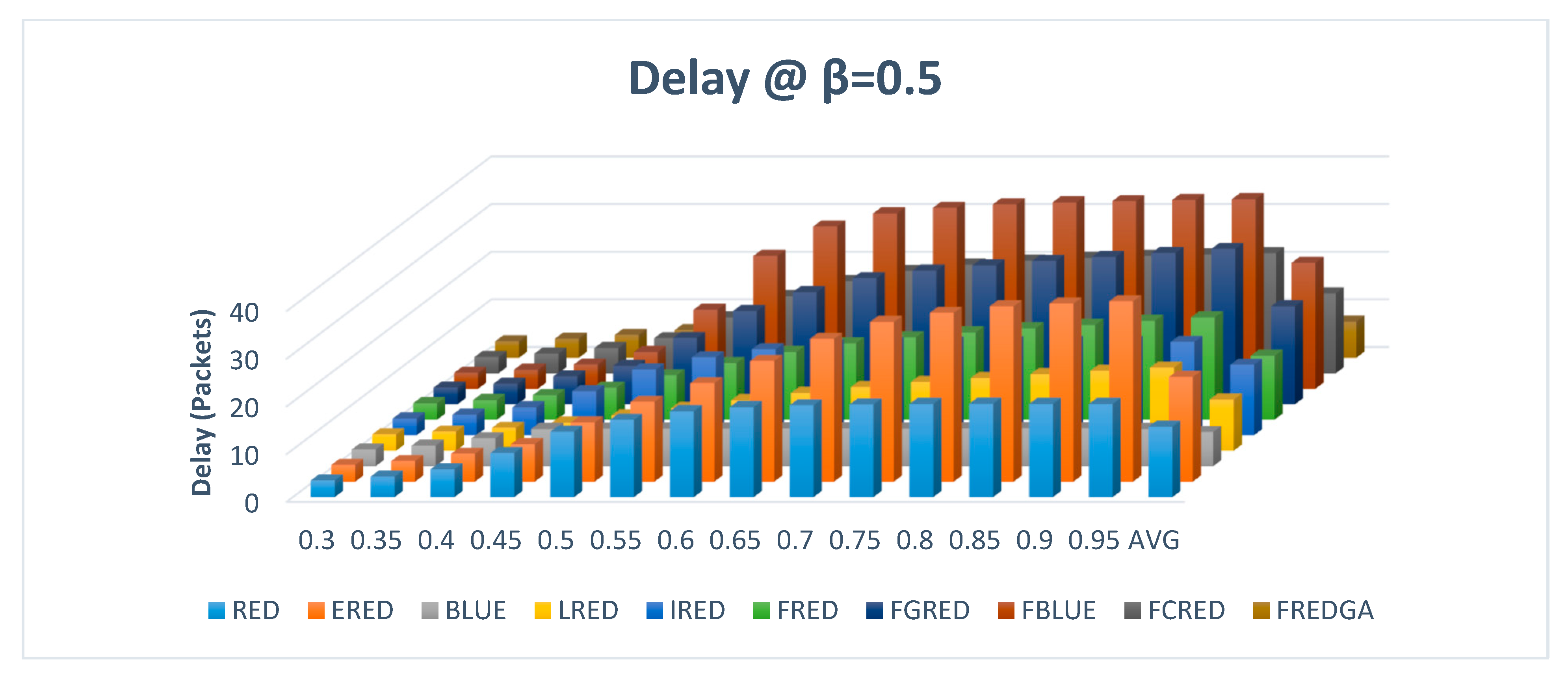
For the dropping, the proposed FREDGA method had a rate of 22%, which is better than the results of the BLUE, which drops an average of 28% of the transmitted packets. As for the rest of the methods that had no loss, LRED, FRED, and FCRED had a drop rate of 21%, which is equivalent to the results obtained by the FREDGA method. However, it was realized that the modest increase in the intended dropping rate of the proposed FREDGA had greatly reduced the delay, as illustrated in Figure 15.

The average delay of the proposed FREDGA method for each packet was 7.57 while it was 10.74 for LRED, 13.42 for FRED, and 16.74 for FCRED. As a result, compared to the best methods, the proposed FREDGA method decreases the delay while maintaining no loss and low drop.

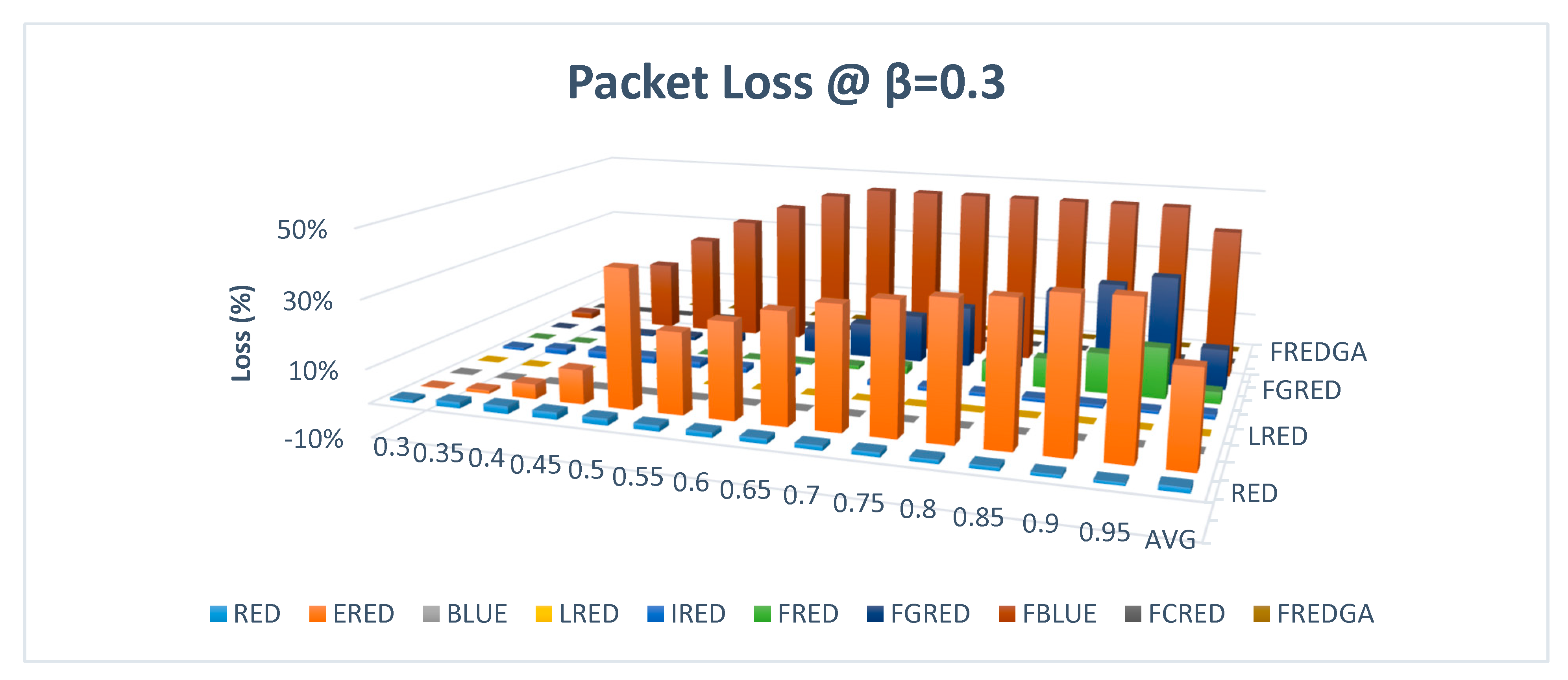
Figure 16 illustrates the loss-based evaluation results under heavy load for the second set of experiments with a low packet departure of 0.3.

As reported in the previous experiment, the results with a more congested network at a departure rate of 0.3 showed that the proposed method FREDGA lost no packets, similar to BLUE, LRED, and FCRED. A significant loss of 44% and 27% of the packets transmitted across the simulated network, respectively, is experienced by the FBLUE and ERED methods. While the FRED method lost 4% of the transmitted packets, FGRED lost 12%, and the RED and IRED methods lost an average of 1%.

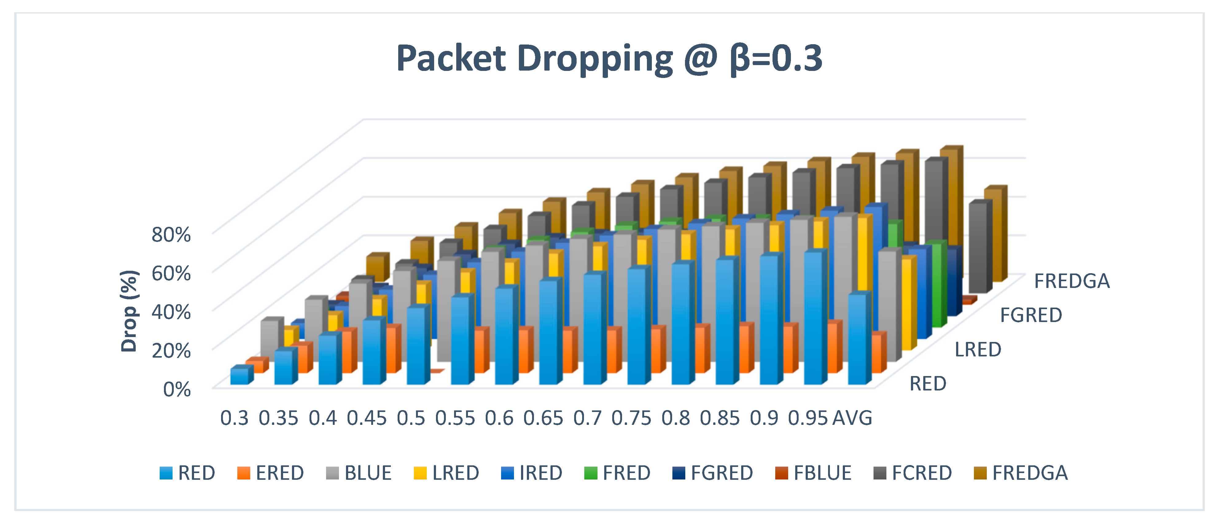
Figure 17 illustrates the evaluation results based on dropping with β value of 0.3 and a single traffic class.

For the dropping rate, in Figure 17, the proposed FREDGA dropped 48% of the transmitted packets while BLUE dropped an average of 57%. As for the rest of the methods, which had no loss, LRED and FCRED dropped 47% and 46% of the packets, respectively. 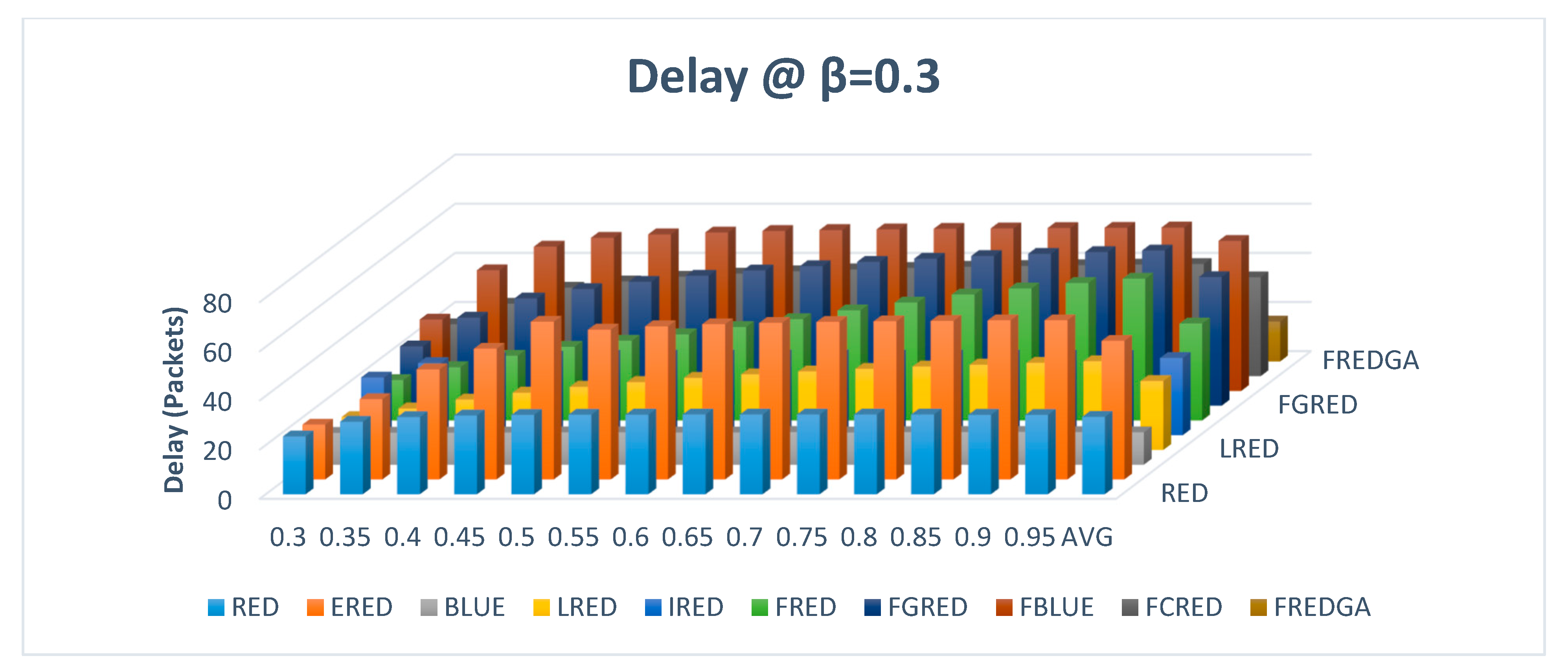Again, it was realized that the modest increase in the intended dropping rate of the proposed FREDGA had greatly reduced the delay, as illustrated in Figure 18.

As given in Figure 18, the average delay of the proposed FREDGA method was 16.23 while it was 28.04 for LRED and 40.23 for FCRED.

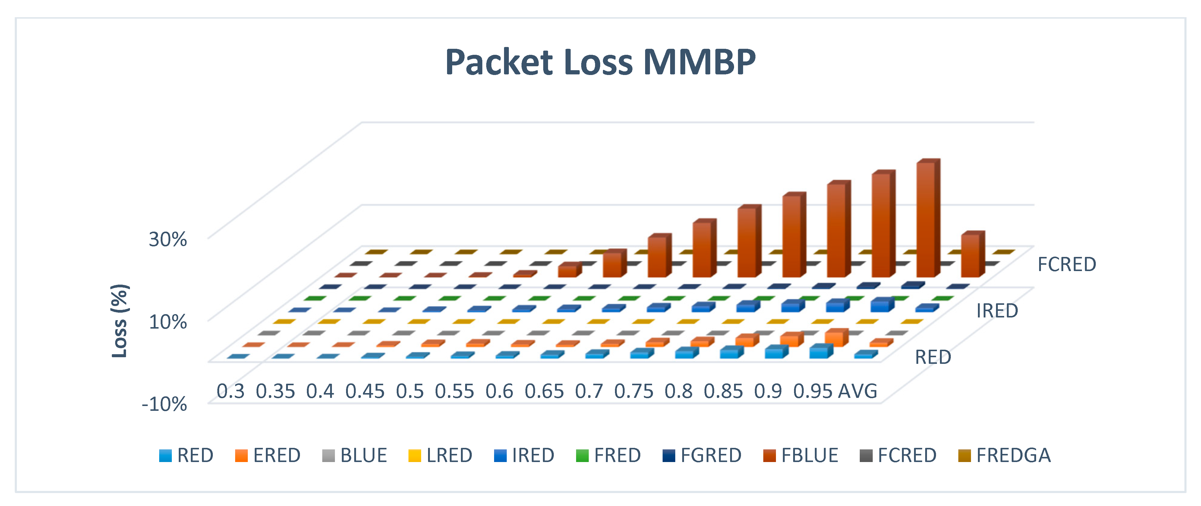
Similarly, for MMBP, the proposed method is implemented and evaluated with various values for the arrival controller α₁, with a single value for α₂ of 0.5 and β set to 0.5. Figure 19 illustrates the evaluation results of the packet loss with 2-stated MMBP.

The results of the MMBP-based simulation confirmed the findings of the previous experiments. For the loss, as illustrated in Figure 19, the proposed FREDGA method did not lose any packets, similar to BLUE, LRED, FRED, FGRED, and FCRED. The FBLUE method suffered a loss of 10% while RED, ERED, and IRED only lost 1% of the transmitted packets.

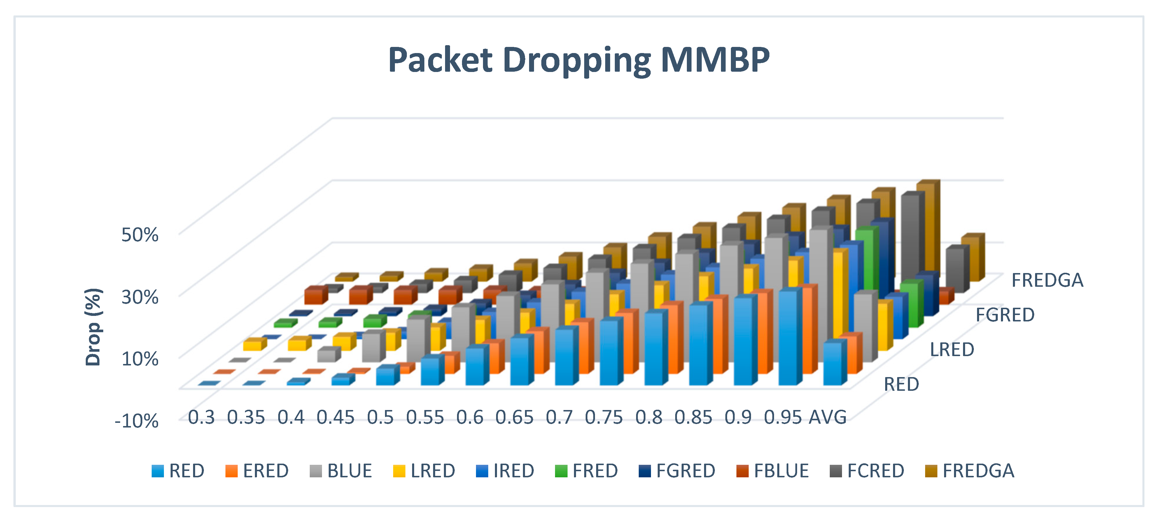
Figure 20 illustrates the evaluation results based on dropping with β value of 0.5 and two-class traffic.

The dropping rate of the proposed FREDGA method is 14%, which is much better than the results of the BLUE, which dropped an average of 22%. As for the rest of the methods that had zero loss, LRED had a dropping rate of 15%, FRED reported a 14% drop, FGRED reported a 13% drop, and FCRED reported a 14% drop.

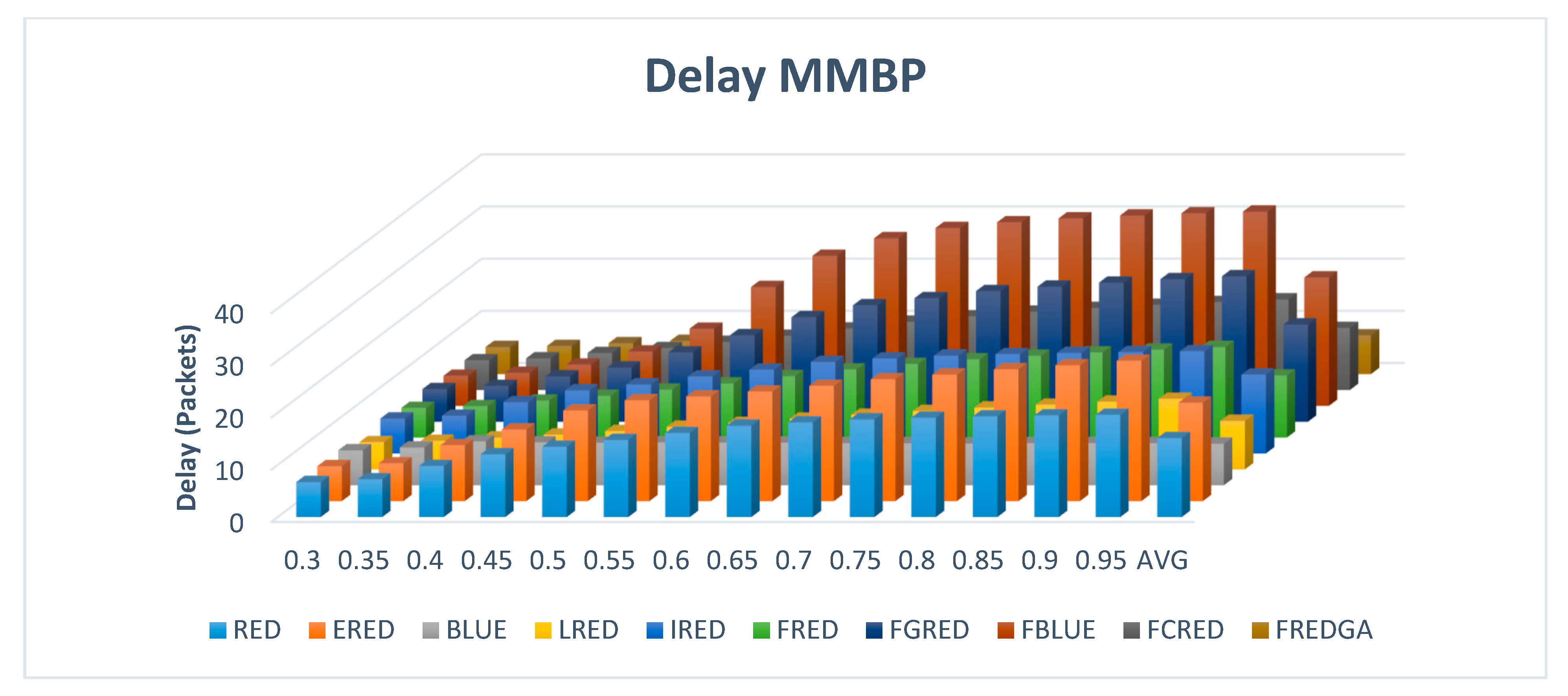
The delay based on dropping with β value of 0.5 and two-class traffic is illustrated in Figure 21.

The average delay of the FREDGA method was 7.43 for each packet, 9.28 for LRED, and 11.9 for FCRED.

The time for running the whole experiment for each method is reported in

Table 8. Running Time Comparison (Per second).

	RED	ERED	BLUE	LRED	IRED	FRED	FGRED	FBLUE	FCRED	FREDGA
β of 0.3	73	61	53	60	59	5840	8440	3801	26,613	942
β of 0.5	73	49	51	61	48	6025	7564	2757	26,882	1155
MMBP	91	77	71	74	76	5342	7015	4643	4289	944

. As noted, the proposed FREDGA required significantly less time compared to the linguistic fuzzy-based methods, excluding the optimization time.

In summary, the proposed FREDGA method improved the delay and maintained zero loss and a low dropping rate compared to the best methods reported in the literature. Moreover, the proposed FREDGA method required significantly less time than the linguistic fuzzy-based methods, reducing the round-trip delay as the processing delay reduced significantly.

5. Conclusions

This paper has proposed a new AQM method based on a precise fuzzy model with GA optimization with a simple buffer counter of the queued packets, Q, as the congestion indicator. The developed adaptive fuzzy-based AQM method aims to stabilize the AQM’s performance. To do so, the proposed method is built on an adaptive calculation for the Dp value. A precise fuzzy model, which replaced the fuzzy linguistic model for AQM, was developed by utilizing GA optimization. The experiments showed that the proposed method outperformed the compared methods in terms of delay and loss with low computational requirements. The delay was improved by 29.5% in moderate single-class traffic, 42.1% in heavy load single-class traffic, and 19.9% in two-class traffic compared to the other methods. Zero loss was maintained in the proposed method, similar to BLUE, FCRED, and LRED, with a good dropping rate that matches FCRED and LRED. The dropping rate was improved by 21.4%, 15.7%, and 36.3% compared to BLUE. The proposed method will be tested in a real-world environment using different models and protocols in the future. Moreover, the proposed method shall be integrated with other counters, such as packet delay and packet loss, to improve the method’s performance, especially during congestion. Moreover, the precise fuzzy model will be used to replace the linguistic model in the state-of-the-art methods, such as the LRED and FCRED, which showed high-performance results.