Effective Modified Fractional Reduced Differential Transform Method for Solving Multi-Term Time-Fractional Wave-Diffusion Equations

Abstract

In this work, we suggest a new method for solving linear multi-term time-fractional wave-diffusion equations, which is named the modified fractional reduced differential transform method (m-FRDTM). The importance of this technique is that it suggests a solution for a multi-term time-fractional equation. Very few techniques have been proposed to solve this type of equation, as will be shown in this paper. To show the effectiveness and efficiency of this proposed method, we introduce two different applications in two-term fractional differential equations. The three-dimensional and two-dimensional plots for different values of the fractional derivative are depicted to compare our results with the exact solutions.

1. Introduction

The fractional derivative (FD) is a generality of the usual differentiation of integer order to non-integer-order fundamental operator ${}_h{\mathbf{D}}_x^{\beta }$, where h and x are the bounds of the operation and $\beta \in \mathbb{R}$. Chen et al. [1] showed the theory of FD and its extensive applications in mechanics and engineering. Important applications of fractional calculus (FC) include vibration and control, anomalous diffusion, continuous-time random walk, non-local phenomena, Levy statistics, and fractional Brownian motion [2]. Different approaches were suggested to answer fractional differential equations (FDE): monotone iterative method, exponential rational function method, homotopy analysis method, and fractional variational iteration method. Symmetry is a major concept in mathematics and physics, and it can be used to shorten the solution of partial differential equations. Iskenderoglu and Kaya [3] considered Lie symmetry analysis of the boundary and initial value problems for partial differential equations with Caputo fractional derivatives.

Several phenomena are defined by fractional (non-integer) derivatives instead of classical (integer) derivatives, for example, using fractional derivatives for the mathematical modeling of viscoelastic materials. Abuasad et al. [4] suggested fractional multi-step differential transformed method (FMsDTM) to catch approximate solutions to the fractional stochastic SIS epidemic model.

The main reason for writing this paper is that there are various techniques established for single-term fractional derivatives, while only a few works in multi-term fractional derivatives are available. There are many practical applications of the time-fractional diffusion-wave equation (TFD-WE). It defines vital physical phenomena which appear in amorphous, glassy, colloidal and porous materials; in fractals and percolating clusters; comb structures; dielectrics and semiconductors; and also appear in polymers, biological systems, random and disordered media, and geophysical and geological processes [5]. Diverse uses for multi-term time-fractional wave-diffusion differential equations have been presented; for example, El-Sayed et al. [6] related the Adomian decomposition method (ADM) with the proposed numerical method (PNM) to explain the multi-term non-linear fractional differential equations. Daftardar-Gejji and Bhalekar [7] resolved fractional multi-term linear and non-linear diffusion-wave equations with ADM. Daftardar-Gejji and Bhalekar [8] used a variable separation technique to solve the equation for multi-term fractional diffusion-wave equations subject to homogeneous and non-homogeneous boundary conditions. Edwards et al. [9] indicated that an approximation of the numerical solution to a multi-term linear FDE can be considered by reducing the problem to a system of ordinary and FDEs each of a max order of one. Jiang et al. [5] explained the multi-term time-fractional diffusion-wave equation by applying the method of separating variables. Katsikadelis [10] established a numerical solution method for solving linear multi-term FDEs; this technique depends on the concept of an analog equation that converts the multi-term to a single-term fractional differential equation with a fictitious source. Pskhua [11] presented an important solution of the multi-time diffusion equation with the Dzhrbashyan–Nersesyan fractional differentiation operator for the time variables. Liu et al. [12] proposed several numerical methods for simulating the two-term mobile/immobile time-fractional diffusion equation, two-term time-fractional wave-diffusion equation, and two computationally effective fractional predictor-corrector methods for the multi-term time-fractional wave-diffusion equations. Li et al. [13] solved a two-dimensional multi-term time-fractional diffusion equation using L1 discretization of each fractional derivative and with a finite difference method. Shen et al. [14] derived an analytical solution to the two-dimensional multi-term time-fractional diffusion and diffusion-wave equation by separating the variables and properties of the multivariate Mittag–Leffler function. Jin et al. [15] examined a space semi-discrete scheme depending on the standard Galerkin finite element technique using continuous piece-wise linear functions. Dehghan et al. [16] proposed a high-order difference method of MT-TFPDEs. Gholami et al. [17] offered a new numerical approach for solutions of single and MT-TFDEs, in which the pseudospectral operational matrix has a critical role. Zheng et al. [18] established a high-order numerical method for MT-TFDEs. Agarwal et al. [19] argued for the existence and uniqueness of solutions to a new class of multi-point and multi-strip boundary value problems of multi-term fractional differential equations using standard fixed point theorems. Katsikadel et al. [20] proposed a new iterative method (NIM) and a modified Adomian decomposition method (MDM) to solve the MT-TFDE with different conditions. Chen et al. [21] presented a unified numerical scheme for solving MT-TFDEs and a class of two-dimensional MT-TFDEs. Zhao et al. [22] suggested the finite element method.

The fractional reduced differential transform method (FRDTM) mainly includes four central stages: firstly, we find the fractional reduced transformed function; secondly, we find the inverse of the fractional reduced transformed function; thirdly, we obtain the approximate the solution; and finally, using special functions, we attempt to discover the exact solution. Gupta [23] suggested different applications to catch the approximate analytical solutions of the Benney–Lin equation with fractional time derivatives using FRDTM and the homotopy perturbation method (HPM). FRDTM was originally proposed by Keskin and Oturance [24]. Different dimensions of non-linear fractional Burgers equations have been solved by Mukhtar et al. [25] using FRDTM. Singh and Srivastava [26] used FRDTM to offer an approximate series solution to the multi-dimensional diffusion equation. Abuasad et al. [27] found the exact and approximate solutions of higher-dimensional time-fractional diffusion equations using FRDTM. Abuasad et al. [28] submitted FRDTM for solving the fractional Helmholtz equation. Saravanan and Magesh [29] connected binary analytical methods, FRDTM vs. FVIM, to obtain numerical solutions for the linear and non-linear Fokker–Planck partial differential equations.

In Section 2, we provide definitions of two types of special functions as well as three types of fractional derivatives. In Section 3, we introduce the definition and properties of the FRDTM and then show four steps of the modified fractional reduced differential transform method for the multi-term time-fractional diffusion-wave equations. Section 4 of this paper focuses on the practical applications and presents semi-analytical results. Two specific examples are explored in this section: the first example involves solving the two-term wave-diffusion equation, while the second example deals with the two-term time-fractional diffusion equation. By examining these cases, we can gain valuable insights into the effectiveness and applicability of the proposed methods. Moving on to Section 5, we reach the conclusion of this paper. In this section, we summarize the main findings and contributions of our study as well as highlight the importance of the results obtained.

2. Preliminaries

Several special functions have captivated the consideration of academics, for example, the Millin–Ross function, the Error function, and the Wright function. We are motivated by two of these special functions. The Mittag–Leffler function holds significant importance in fractional calculus as it is frequently employed to express solutions in a concise manner. By utilizing the definition of the Mittag–Leffler function, we can obtain the exact solution after obtaining it in a compact form. Furthermore, the Gamma function plays a vital role in defining fractional-order operations and is an integral component of the fractional calculus framework.

2.1. Mittag–Leffler Function

The Mittag–Leffler (M-L) function is a generality of the familiar exponential function ${\mathrm{e}}^x$. The one-parameter M-L function, represented in powers series, is [30]

$$E_{\gamma }\left(x\right)=\sum _{k=0}^{\infty }\frac{x^k}{\Gamma (\gamma k+1)},\gamma >0.$$

For particular integer values of $\gamma$, we obtain

$$\begin{array}{ccc}& & E_0\left(x\right)=\frac{1}{1-z},E_1\left(x\right)={\mathrm{e}}^x,\hfill \\ & & E_2\left(x\right)=cosh\left(\sqrt{x}\right).\hfill \end{array}$$

While the two-parameter M-L function can be defined as

$$E_{\gamma ,\beta }\left(x\right)=\sum _{k=0}^{\infty }\frac{x^k}{\Gamma (\gamma k+\beta )},\gamma >0,\mathrm{and}\beta >0.$$

For distinct selections of the two parameters, $\gamma$ and $\beta$, we gain the well-known traditional functions

$$\begin{array}{ccc}& & E_{1,1}\left(x\right)=E_1\left(x\right)={\mathrm{e}}^x,E_{1,2}\left(x\right)=\frac{e^x-1}{x},\hfill \\ & & E_{2,1}\left(x^2\right)=cosh\left(x\right),E_{2,2}\left(x^2\right)=\frac{sinh\left(x\right)}{x}.\hfill \end{array}$$

2.2. The Gamma Function

The Gamma function, $\Gamma \left(z\right)$, extends the concept of factorials to real arguments. The Gamma function can be defined as [30]

$$\Gamma \left(z\right)={\int }_0^{\infty }{e}^{-t}{t}^{z-1}dt,z>0,$$

which is convergent on the right side of the complex plane $\Re \left(z\right)>0$.

2.3. Fractional Derivative

Several special definitions are presented for the fractional derivative. The commonly used definitions for the overall fractional derivatives are the Riemann–Liouville (RL), the Grünwald–Letnikov operator (GLO), and the well-known Caputo definition [30,31,32].

2.3.1. Grünwald–Letnikov Operator

The Grünwald–Letnikov operator (GLO) is given as

$${}_a{\mathbf{D}}_t^{\alpha }f\left(t\right)=\underset{h\to 0}{lim}{h}^{-\alpha }\sum _{j=o}^{\left[\frac{t-\alpha }{h}\right]}{(-1)}^j\left(\begin{array}{c}\alpha \\ j\end{array}\right)f(t-jh),$$

where $[.]$ means the integer part, which represents the derivative of order m in the case when $\alpha =m$, and the m-fold integral in the case when $\alpha =-m$.

2.3.2. Riemann–Liouville Derivative

The Riemann–Liouville (RL) derivative is defined as [33]

$${\mathbf{D}}_a^{\alpha }f\left(t\right)=\left\{\begin{array}{cc}{\displaystyle \frac{1}{\Gamma (n-\alpha )}\frac{d^n}{d{t}^n}{\int }_a^t\frac{f\left(\tau \right)}{{(t-\tau )}^{\alpha +1-n}}d\tau ,}\hfill & n-1<\alpha <n,\hfill \\ \\ {\displaystyle \frac{d^n}{d{t}^n}f\left(t\right),}\hfill & \alpha =n,\hfill \end{array}\right.$$

where $n\in \mathbb{N}$, $\mathbb{N}$ is the set of all natural numbers, and $\alpha >0,t>a$, with $\alpha ,a,t\in \mathbb{R}$, where $\mathbb{R}$ represents the set of all real numbers.

2.3.3. Caputo Fractional Derivative

The Caputo fractional derivative is defined as [34]

$${}^c{\mathbf{D}}_t^{\alpha }g\left(t\right):=\left\{\begin{array}{cc}{\displaystyle \frac{1}{\Gamma (n-\alpha )}{\int }_a^t\frac{g^{\left(n\right)}\left(\tau \right)}{{(t-\tau )}^{\alpha +1-n}}d\tau ,}\hfill & n-1<\alpha <n,\hfill \\ \\ {\displaystyle \frac{d^n}{d{t}^n}g\left(t\right),}\hfill & \alpha =n,\hfill \end{array}\right.$$

where $n\in \mathbb{N}$, and $\alpha >0,t>a$, with $\alpha ,a,t\in \mathbb{R}$. The small c in the top left of ${}^c\mathbf{D}$ refers to the Caputo fractional derivative.

2.3.4. Relation between the Riemann–Liouville Operator and Caputo Operator

The relation between the RL operator and Caputo operator is given by [23]

$${}^c{\mathbf{D}}_a^{\beta }w(x,t)={\mathbf{D}}_a^{\beta }\left[w(x,t)-\sum _{h=0}^{n-1}{u}^h(x,a)\frac{{(t-a)}^h}{h!}\right].$$

3. Fractional Reduced Differential Transform Method (FRDTM)

To explain the FRDTM, we provide its essential definitions and necessary properties. Consider a function of $(n+1)$ variables $\mu (t,x_1,x_2,\dots ,x_n)$, such that

$$\mu (t,x_1,x_2,\dots ,x_n)={\mu }_1\left(x_1\right){\mu }_2\left(x_2\right)\cdots {\mu }_n\left(x_n\right)h\left(t\right),$$

then we have, from the properties of the one-dimensional differential transform method (DTM), that

$$\begin{array}{ccc}\hfill \mu (t,x_1,x_2,\dots ,x_n)& =& \sum _{i_1=0}^{\infty }{\mu }_1\left(i_1\right)x_1^{i_1}\cdots \sum _{i_n=0}^{\infty }{\mu }_n\left(i_n\right)x_n^{i_n}\sum _{j=0}^{\infty }h\left(j\right)t^j\hfill \\ & =& \sum _{i_1=0}^{\infty }\cdots \sum _{i_n=0}^{\infty }\sum _{j=0}^{\infty }{M}_k(i_1,\dots ,i_n,j)x_1^{i_1}\cdots x_n^{i_n}{t}^j,\hfill \end{array}$$

where $M_k(i_1,i_2,\dots ,i_n,j)={\mu }_1\left(i_1\right){\mu }_2\left(i_2\right)\cdots {\mu }_n\left(i_n\right)h\left(j\right)$ is referred to as the spectrum of $\mu (t,x_1,x_2,\dots ,x_n)$, for $k=0,1,2,\dots$. Furthermore, the lowercase $\mu (t,x_1,x_2,\dots ,x_n)$ is used to represent the original function, while its fractional reduced transformed function is represented by the uppercase $M_k(x_1,\dots ,x_n)$, which is called the T-function.

Table 1. Fundamental operations of the FRDTM [28,35,36,37].

Original Function	Transformed Function
$c_1\mu \pm c_2\tau$	$c_1{M}_k\pm c_2{T}_k$
$\mu \tau$	${\sum }_{i=0}^k{M}_i{T}_{k-i}$
${\displaystyle {\mathbf{D}}_t^{m\alpha }\mu }$	${\displaystyle \frac{\Gamma (k\alpha +m\alpha +1)}{\Gamma (k\alpha +1)}M(k+m)}$
${\displaystyle \frac{{\partial }^h\mu }{\partial x_i^h}}$	${\displaystyle \frac{{\partial }^h{M}_k}{\partial x_i^h}}$, $i=1,2,\dots ,n$
$x_i^m{t}^r$	$x_i^m\delta (k-r)$, $i=1,2,\dots ,n$
$x_i^m{t}^r\mu$	${\displaystyle x_i^m{M}_{k-r}}$, $i=1,2,\dots ,n$

provides the specific properties of the FRDTM, where $\delta (a-b)$ is

$$\delta (a-b)=\left\{\begin{array}{cc}1,\hfill & a=b,\hfill \\ 0,\hfill & a\ne b,\hfill \end{array}\right.$$

where $\tau =\tau (t,x_1,x_2,\dots ,x_n)$, $\mu =\mu (t,x_1,x_2...,x_n)$, $T_k=T_k(x_1,x_2,\dots ,x_n)$, and $M_k=M_k(x_1,x_2,\dots ,x_n).$

Modified Fractional Reduced Differential Transform Method for Multi-Term Time-Fractional Diffusion-Wave Equations

In this part, we present the introduction of the Fractional Reduced Differential Transform Method (FRDTM) for multi-term time-fractional diffusion-wave equations. Previous studies [26,27,28,36,38] have proposed the FRDTM for single-term time-fractional equations; however, Abuasad et al. [39] suggested a new modification to the FRDTM, specifically tailored for non-homogeneous linear multi-term time-fractional diffusion equations (MT-TFDEs) with constant coefficients in a certain bounded domain and appropriate initial conditions. This modified approach, known as the modified fractional reduced differential transform method (m-FRDTM), allows for the exact and approximate solutions of MT-TFDEs to be obtained. We need to test more applications to ensure that this modified method is effective for different types of multi-term time-fractional diffusion-wave equations.

$$\sum _{i=1}^n{\mathbf{D}}_t^{{\alpha }_i}\mu (t,X)+a\frac{{\partial }^{\beta }\mu (t,X)}{\partial t^{\beta }}=b\sum _{j=1}^m\frac{{\partial }^2\mu (t,X)}{\partial x_j^2}+g(t,X),$$

(1)

where $X=(x_1,x_2,\dots ,x_m)$; $n,m$ and $\beta$ are natural numbers; $0\le t\le T$, $T\in {\mathbb{R}}^{+}$, where ${\mathbb{R}}^{+}$ is the set of positive real numbers; $0\le x_j\le L$, $j=1,2,\cdots ,m$, where $L\in {\mathbb{R}}^{+}$; and ${\alpha }_i>0$, $i=1,2,\cdots ,n$, with the initial condition $\mu (0,X)={\mu }_0(t,X)$ and the arbitrary integer constants a and b, not both of them equal zero.

Equation (1) represents the time-fractional diffusion-wave equation if $1<{\alpha }_i<2$ and a fractional diffusion equation if $0<{\alpha }_i<1$. When ${\alpha }_i=2$, Equation (1) represents a traditional wave equation, while if ${\alpha }_i=1$ it represents a traditional diffusion equation.

There are four steps for solving the multi-term time-fractional wave-diffusion equations using m-FRDTM:

Step 1: 

Finding the Fractional Reduced Transformed Function (FRTF)

Let $\mu (t,X)$ be an analytical and continuously differentiable with respect to $m+1$ variables t and X in the specified domain D; thus, the m–FRDTM in m-dimensions of $\mu (t,X)$ is given by

$$M_k\left(X\right)=\frac{1}{\Gamma (k{\sum }_{i=1}^n{\alpha }_i+1)}{\left[\sum _{i=1}^n{\mathbf{D}}_t^{{\alpha }_{i}k}\left(\mu (t,X)\right)\right]}_{t=t_0},$$

(2)

where $k=0,1,2,\dots$.

Step 2: 

Finding the Inverse of FRTF

The inverse FRDTM of $M_k\left(X\right)$ is defined by

$$\mu (t,X):=\sum _{k=0}^{\infty }{M}_k\left(X\right){(t-t_0)}^{k{\sum }_{i=1}^n{\alpha }_i}.$$

(3)

By substituting Equation (2) into Equation (3), we obtain

$$\mu (t,X)=\sum _{k=0}^{\infty }\frac{1}{\Gamma (k{\sum }_{i=1}^n{\alpha }_i+1)}{\left[\sum _{i=1}^n{\mathbf{D}}_t^{{\alpha }_{i}k}\left(\mu (t,X)\right)\right]}_{t=t_0}{(t-t_0)}^{k{\sum }_{i=1}^n{\alpha }_i}.$$

In particular, for $t_0=0$, the above formula becomes

$$\mu (t,X)=\sum _{k=0}^{\infty }\frac{1}{\Gamma (k{\sum }_{i=1}^n{\alpha }_i+1)}{\left[\sum _{i=1}^n{\mathbf{D}}_t^{{\alpha }_{i}k}\left(\mu (t,X)\right)\right]}_{t=0}{t}^{k{\sum }_{i=1}^n{\alpha }_i}.$$

Step 3: 

Finding the Approximate Solution

The inverse transformation of the set of values ${\left\{M_k\left(X\right)\right\}}_{k=0}^z$, where $z=0,1,2,\dots$, offers the approximate solution of the function $\mu (t,X)$ as a finite power series, where z represents the order of the approximate solution

$${\tilde{\mu }}_z(t,X)=\sum _{k=0}^z{M}_k\left(X\right)t^{k{\sum }_{i=1}^n{\alpha }_i},$$

(4)

where $M_k\left(X\right)$ in (4) for MT-TFDE (1) can be described as

$$\begin{array}{c}\sum _{i=1}^n\frac{\Gamma (k{\alpha }_i+1)}{\Gamma ((k-1){\alpha }_i+1)}{M}_k\left(X\right)+a\frac{\Gamma (k\beta +1)}{\Gamma \left(\right(k-1)\beta +1)}{M}_k\left(X\right)=\hfill \\ \hspace{1em}\hspace{1em}\hspace{1em}\hspace{1em}\hspace{1em}\hspace{1em}\hspace{1em}\hspace{1em}\hspace{1em}\hspace{1em}\hspace{1em}\hspace{1em}\hspace{1em}\hspace{1em}\hspace{1em}\hspace{1em}\hspace{1em}\hspace{1em}\hspace{1em}\hspace{1em}b\sum _{j=1}^m\frac{{\partial }^2{M}_{(k-1)}\left(X\right)}{\partial x_j^2}+G\left(X\right),\hfill \end{array}$$

where $G\left(X\right)$ represents the FRDTM of $g(t,X)$ and can be established from Table 1.

Step 4: 

Finding the Exact Solution

The exact solution by means of the m-FRDTM is specified by

$$\mu (t,X)=\underset{z\to \infty }{lim}{\tilde{\mu }}_z(t,X).$$

4. Semi-Analytical Examples

In this section, we present two examples, first for a two-term wave-diffusion equation and the other for a two-term time-fractional diffusion equation. This is to show the importance and effectiveness of the m-FRDTM in solving different types of multi-term time-fractional wave-diffusion equations.

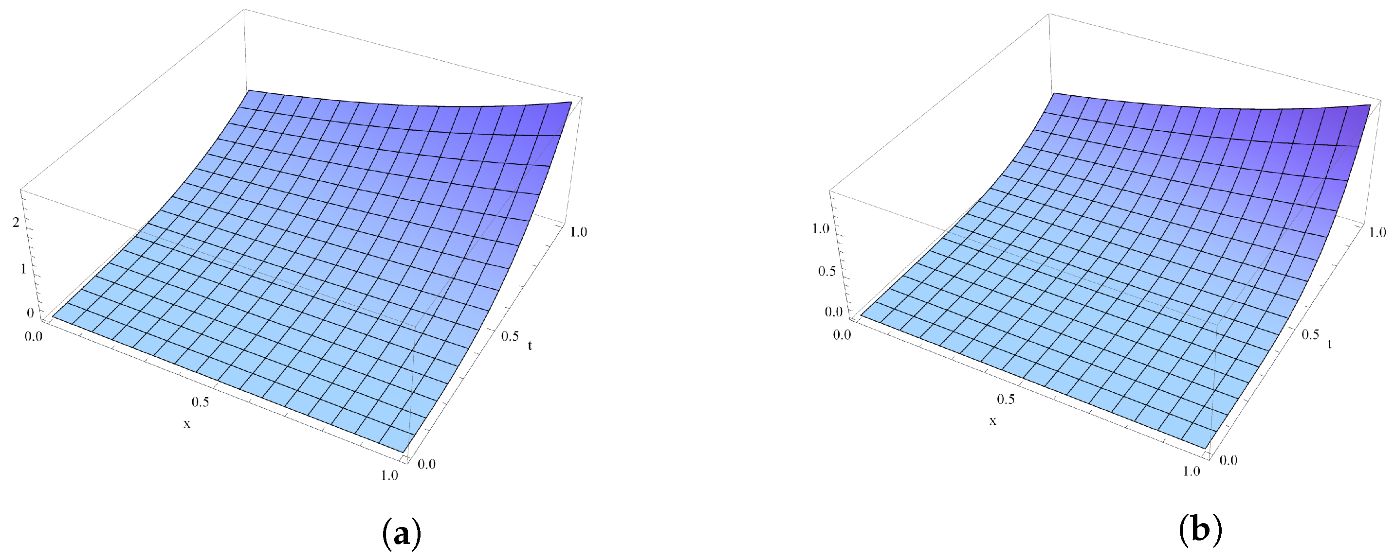
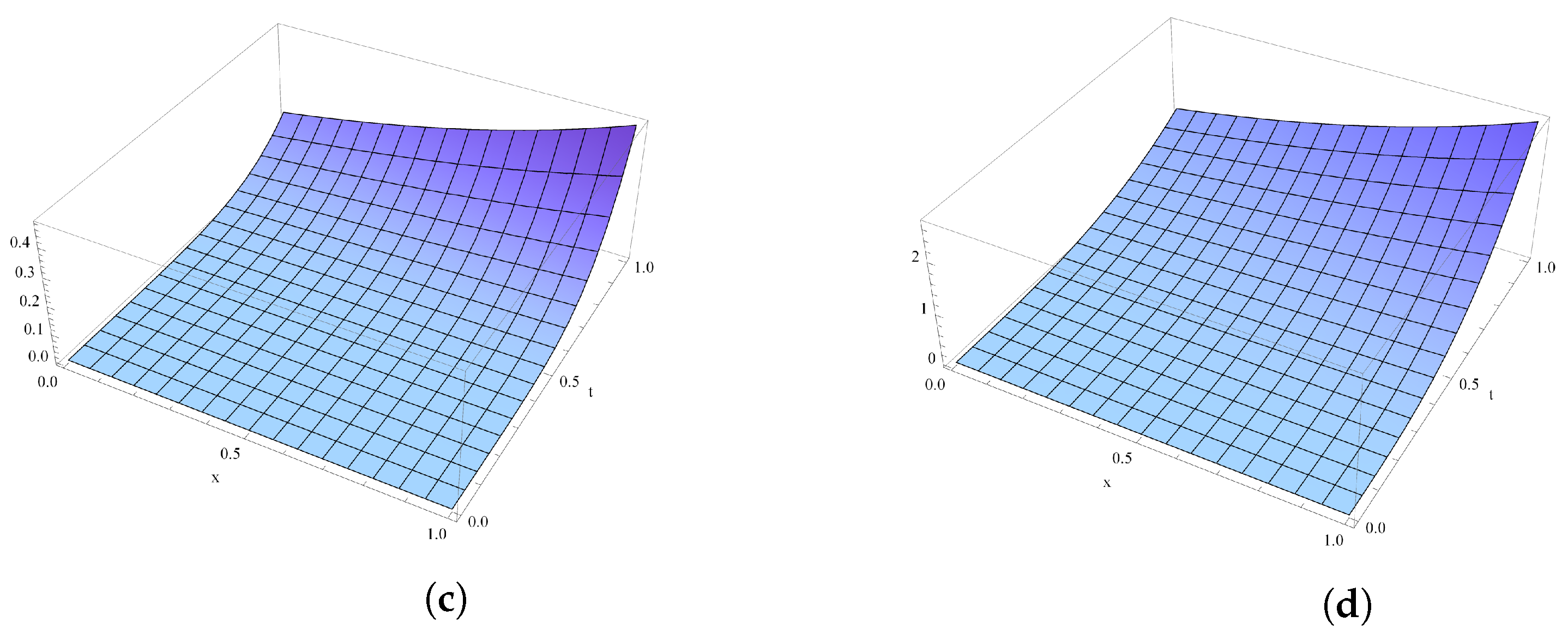
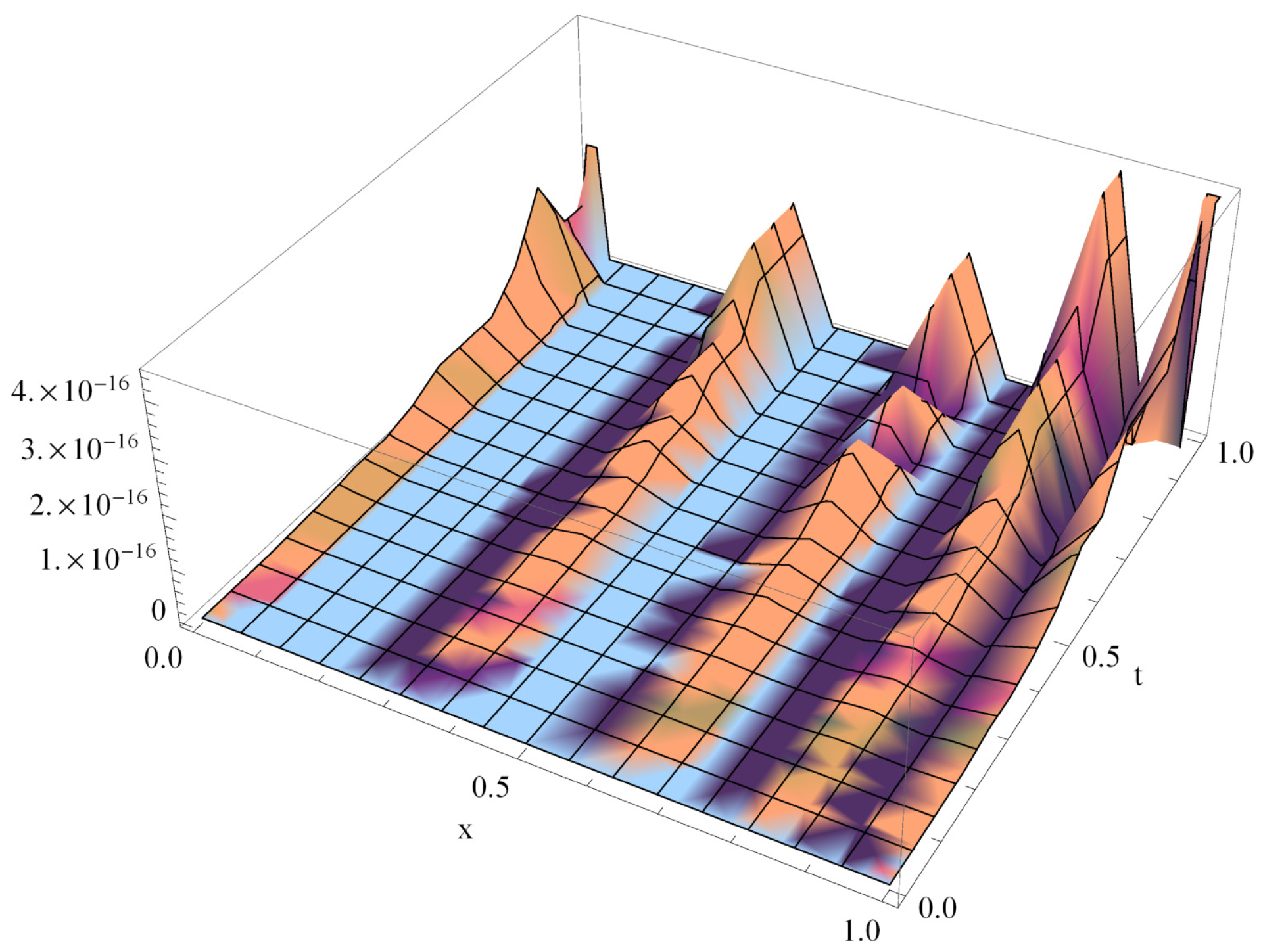
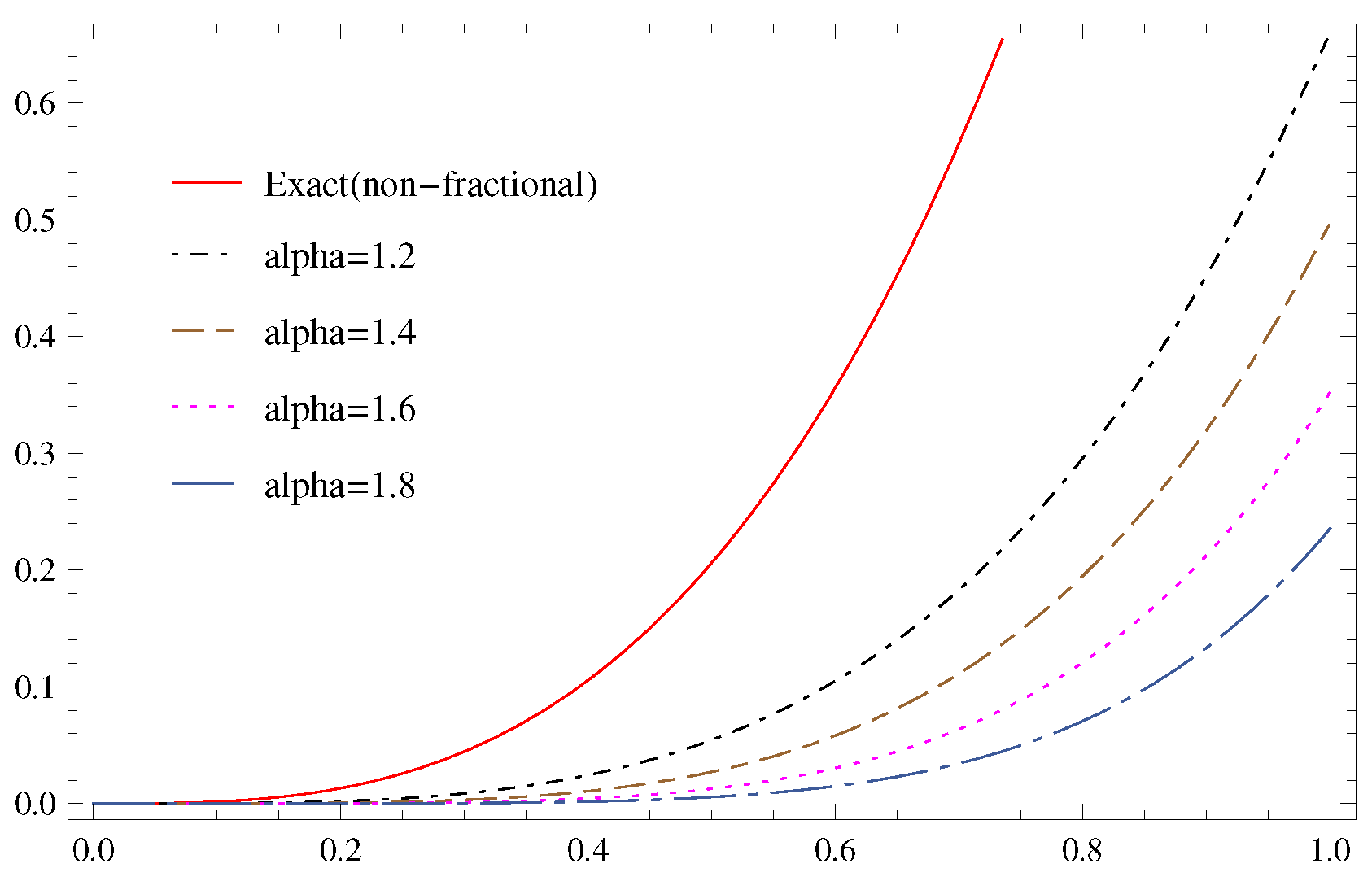
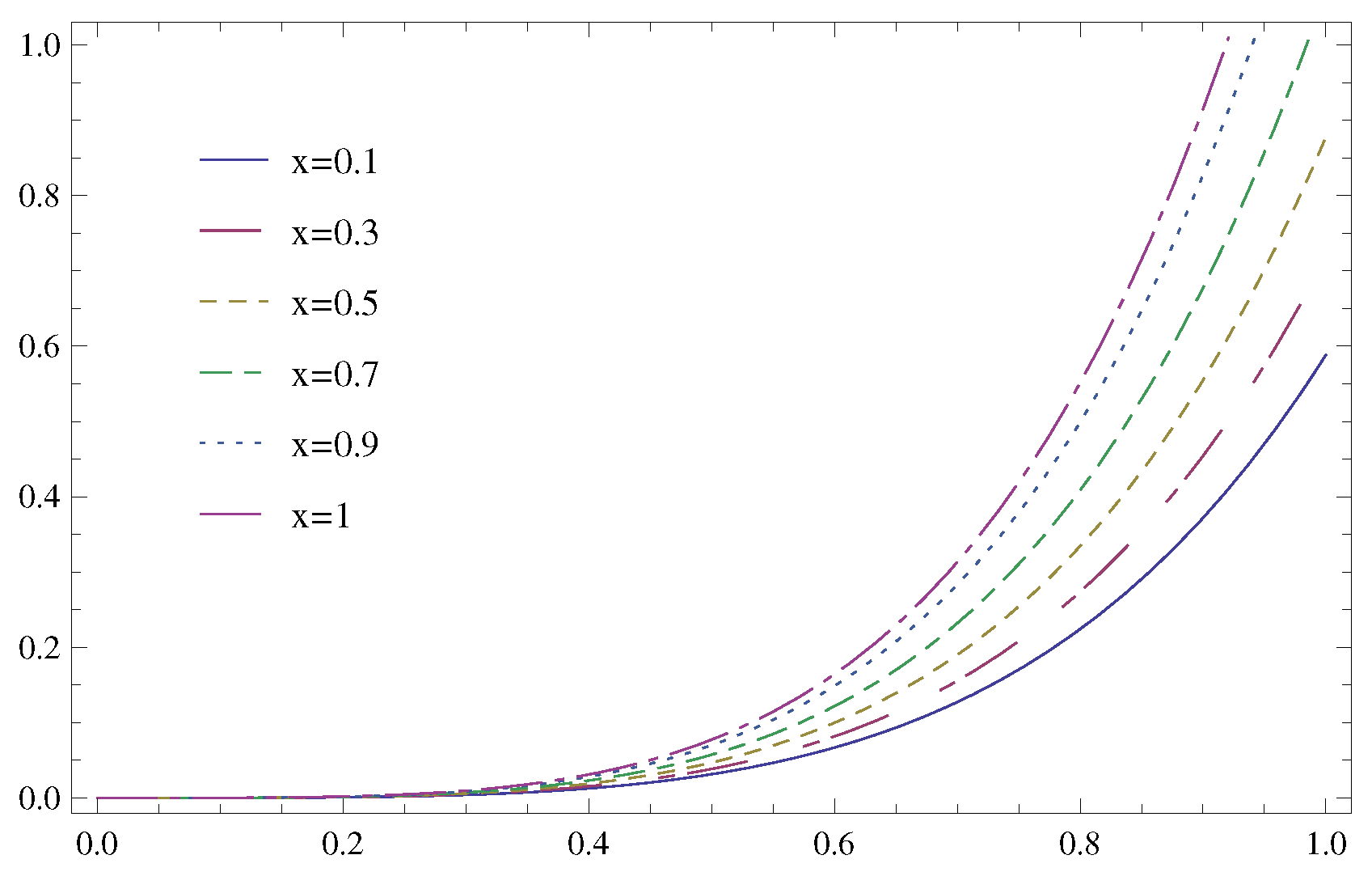
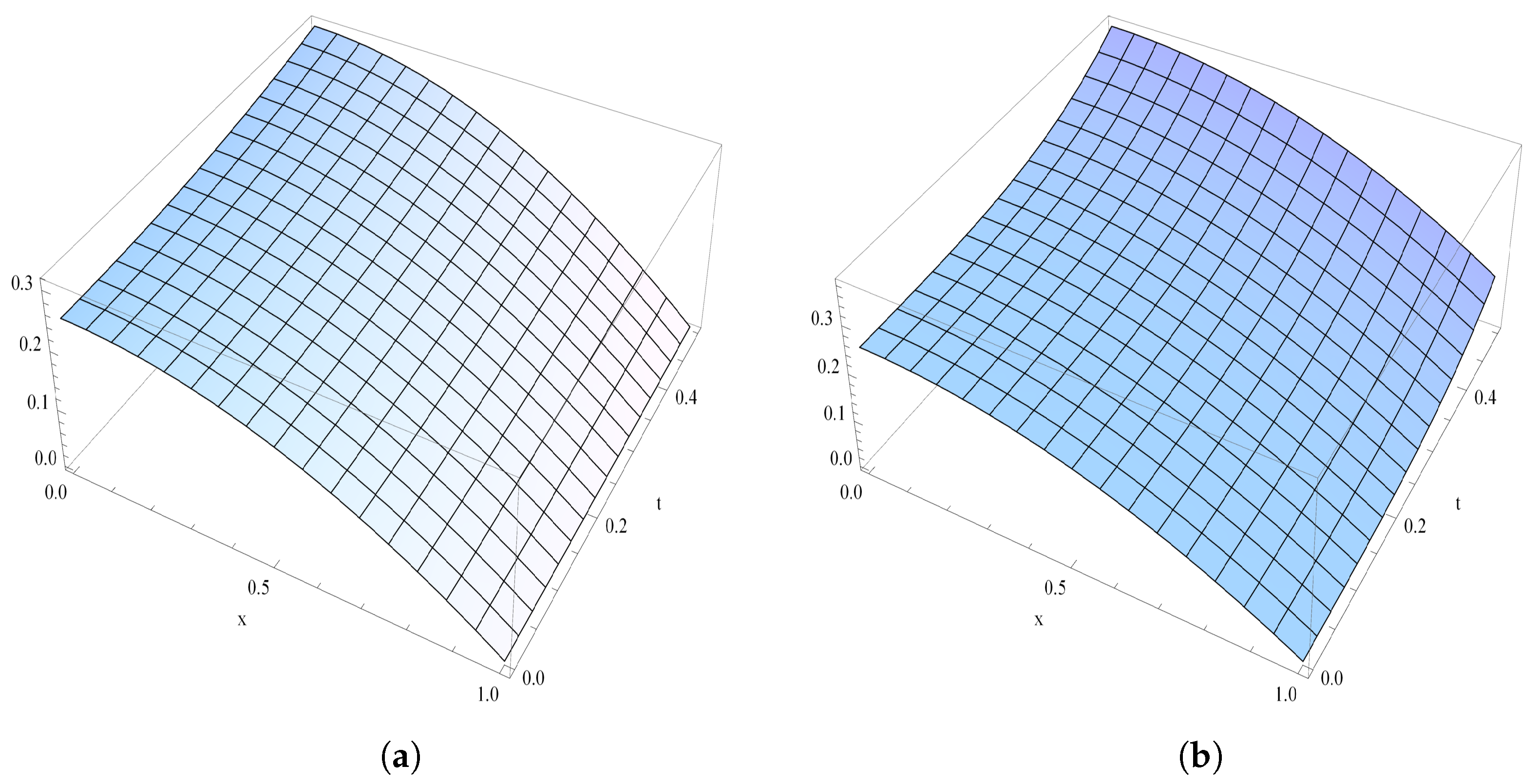
4.1. Example 1: (Two-Term Wave-Diffusion Equation)

Let this two-term wave-diffusion equation possess damping with $1\le \alpha <2$:

$${\mathbf{D}}_t^{\alpha }\mu (x,t)+\frac{\partial \mu (x,t)}{\partial t}=\frac{{\partial }^2\mu (x,t)}{\partial x^2}+g(x,t),$$

(5)

subject to the initial condition (I.C.)

$$\mu (x,0)={\mu }_0(x,t)=0,$$

(6)

where $t\in [0,1]$, $x\in [0,1]$, and

$$g(x,t)=\left(3t^2-t^3+\frac{6t^{3-\alpha }}{\Gamma (4-\alpha )}\right){\mathrm{e}}^x.$$

Applying the properties from Table 1 to Equation (5), we obtain the recurrence relation

$$\begin{array}{ccc}\hfill M_{k+1}\left(x\right)& =& \frac{\Gamma (k\alpha +1)}{(k+1)\Gamma (k\alpha +1)+\Gamma \left(\right(k+1)\alpha +1)}(\frac{{\partial }^2{M}_k\left(x\right)}{\partial x^2}\hfill \\ & & +2{\mathrm{e}}^x\delta (k-1)-{\mathrm{e}}^x\delta (k-2)+\frac{2{\mathrm{e}}^x\delta (k-2+\alpha )}{\Gamma (3-\alpha )}),\hfill \end{array}$$

(7)

for $k=0,1,2,\dots$.

From Equation (7), the inverse transform coefficients of $t^{k\alpha }$ are set as

$$\begin{array}{ccc}\hfill U_0\left(x\right)& =& 0,\hfill \\ \hfill U_1\left(x\right)& =& \left\{\begin{array}{cc}{\displaystyle \frac{6e^x}{7},}& \alpha =3,\\ {\displaystyle 0,}& \mathrm{True},\end{array}\right.\hfill \\ \hfill U_2\left(x\right)& =& \left\{\begin{array}{cc}{\displaystyle \frac{3e^x}{7},}& \alpha =2,\\ & \\ {\displaystyle \frac{3e^x}{427},}& \alpha =3,\\ & \\ 0& \mathrm{True},\end{array}\right.\hfill \\ \hfill U_3\left(x\right)& =& \left\{\begin{array}{cc}{\displaystyle \frac{428e^x}{72163},}& \alpha =3,\\ & \\ {\displaystyle \frac{8e^x}{77},}& \alpha =2,\\ & \\ {\displaystyle e^x,}& \alpha =1,\\ & \\ {\displaystyle \frac{3e^x\Gamma (2\alpha +1)}{3\Gamma (2\alpha +1)+\Gamma (3\alpha +1)},}& \mathrm{True},\end{array}\right.\hfill \\ & & ⋮.\hfill \end{array}$$

After a few number of iterations, the differential inverse transform of ${\left\{M_k\right\}}_{k=0}^{\infty }$ provides the resulting series of solutions

$$\begin{array}{ccc}\hfill \mu (x,t)& =& \sum _{k=0}^{\infty }{M}_k\left(x\right)t^{k\alpha },\hfill \\ & =& M_0\left(x\right)+M_1\left(x\right)t^{\alpha }+M_2\left(x\right)t^{2\alpha }+M_3\left(x\right)t^{3\alpha }+\cdots ,\hfill \end{array}$$

(8)

$$\begin{array}{ccc}\hfill {\mu }_3(x,t)& =& \left\{\begin{array}{cc}{\displaystyle \frac{3e^x}{4},}\hfill & \alpha =0,\hfill \\ & \\ {\displaystyle t^3{e}^x,}\hfill & \alpha =1,\hfill \\ & \\ {\displaystyle \frac{1}{77}{t}^4\left(8t^2+33\right)e^x,}\hfill & \alpha =2,\hfill \\ & \\ {\displaystyle \frac{3e^x\Gamma (2\alpha +1)}{3\Gamma (2\alpha +1)+\Gamma (3\alpha +1)},}\hfill & \alpha \ne 0,\alpha \ne 1,\alpha \ne 2.\hfill \end{array}\right.\hfill \end{array}$$

If $\alpha =1$, then the m-FRDTM solution (8) gives the exact solution of the non-fractional diffusion equation in (5), subject to the initial conditions in (6)

$$\mu (x,t)=t^3{e}^x,$$

which is the matching outcome achieved in [12]; while for the fractional-order, we can obtain the approximate solutions for different selected values of $\alpha$:

$$\begin{array}{ccc}\hfill {\mu }_3(x,t)& =& 0.114609t^{5.7}{e}^x,\alpha =1.9,\hfill \\ \hfill {\mu }_3(x,t)& =& 0.175913t^{5.1}{e}^x,\alpha =1.7,\hfill \\ \hfill {\mu }_3(x,t)& =& 0.25589t^{4.5}{e}^x,\alpha =1.5,\hfill \\ \hfill {\mu }_3(x,t)& =& 0.350459t^{3.9}{e}^x,\alpha =1.3,\hfill \\ \hfill {\mu }_3(x,t)& =& 0.450908t^{3.3}{e}^x,\alpha =1.1.\hfill \end{array}$$

We can write the general form of the approximate solutions of the problem in (5), subject to the initial condition in (6), as

$${\mu }_3(x,t)=a{t}^{3\left(\alpha \right)}{e}^x,1\le \alpha <2,$$

where $a\in {\mathbb{R}}^{+}$, $0\le a\le 1$.

To clarify the results for the example in Section 4.1, it is possible to compare the non-fractional exact solution with the approximate solutions for m-FRDTM with a three-dimensional drawing of different selected values of fractional order $\alpha$ ($\alpha =2,1.7,1$) in Figure 1. It is also appropriate to draw the absolute error between the exact solution and the three-term approximate solution for m-FRDTM (when $\alpha =1$) in Figure 2. The figure clearly shows that the maximum absolute error is $4\times {10}^{-16}$, while to compare our results in the two-dimensional plot for the approximate solutions of different values of $\alpha$ and the exact solution of non-fractional order, we plot Figure 3. The approximate solutions in the two-dimensional schemes for $\alpha =2$ are shown for different values of x in Figure 4.

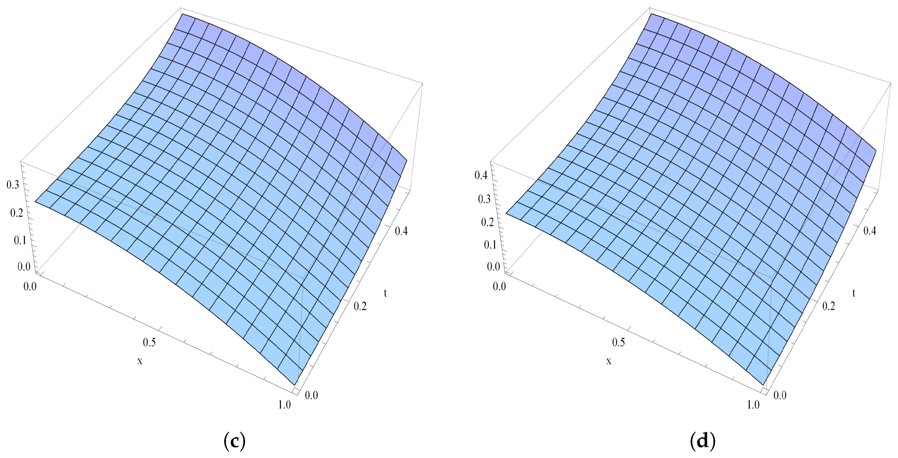
4.2. Example 2: (Two-Term Time-Fractional Diffusion Equation)

Consider the two-term time-fractional diffusion equation [17]

$${\mathbf{D}}_t^{{\alpha }_1}\mu (x,t)+{\mathbf{D}}_t^{{\alpha }_2}\mu (x,t)-4\frac{{\partial }^2\mu (x,t)}{\partial x^2}=f(x,t),(x,t)\in [-1,1]\times [0,1],$$

(9)

subject to the initial condition

$$\mu (x,0)={\mu }_0(x,t)=\frac{1}{4}\left(1-x^2\right),$$

(10)

where $0\le {\alpha }_i<1$, $i=1,2$ and

$$f(x,t)=\frac{t^{2-{\alpha }_1}}{\Gamma (3-{\alpha }_1)}\left(\frac{1-x^2}{2}\right)+\frac{t^{2-{\alpha }_2}}{\Gamma (3-{\alpha }_2)}\left(\frac{1-x^2}{2}\right)+2(1+t^2).$$

Using the right properties from Table 1 in Equation (9), we obtain the resulting recurrence relation

$$\begin{array}{ccc}\hfill M_{k+1}\left(x\right)& =& \frac{\Gamma (k{\alpha }_1+1)\Gamma (k{\alpha }_2+1)}{\Gamma ((k+1){\alpha }_1+1)\Gamma (k{\alpha }_2+1)+\Gamma (k{\alpha }_1+1)\Gamma ((k+1){\alpha }_1+1)}\hfill \\ & & \times [\frac{1}{2}\left(1-x^2\right)\left(\frac{\delta (k+1,3-\alpha )}{\Gamma (3-\alpha )}+\frac{\delta (k+1,3-\beta )}{\Gamma (3-\beta )}\right)\hfill \\ & & +2(\delta (k+1,3)+1)+4\frac{{\partial }^{2}M\left(k\right)}{\partial x\partial x}],\hfill \end{array}$$

(11)

where $k=0,1,2,\dots$.

From Equation (11), we obtain the inverse transform coefficients of $t^{k({\alpha }_1+{\alpha }_2)}$ as follows:

$$\begin{array}{ccc}\hfill M_0\left(x\right)& =& {\displaystyle \frac{1}{4}\left(1-x^2\right),}\hfill \\ \\ \hfill M_1\left(x\right)& =& 0,({\alpha }_1=0\wedge {\alpha }_2=1)\vee ({\alpha }_1=1\wedge {\alpha }_2=0),\hfill \\ \\ \hfill M_2\left(x\right)& =& \left\{\begin{array}{cc}{\displaystyle \frac{1}{6}\left(5-x^2\right),}\hfill & ({\alpha }_1=0\wedge {\alpha }_2=1)\vee ({\alpha }_1=1\wedge {\alpha }_2=0),\hfill \\ & \\ {\displaystyle \frac{1}{4}\left(3-x^2\right),}\hfill & {\alpha }_1={\alpha }_2=1,\hfill \\ & \\ {\displaystyle -\frac{{\alpha }_2\left(x^2-5\right)\Gamma \left({\alpha }_2\right)}{2(2\Gamma ({\alpha }_2+1)+\Gamma (2{\alpha }_2+1))},}\hfill & {\alpha }_1=1,\hfill \\ & \\ {\displaystyle -\frac{{\alpha }_1\left(x^2-5\right)\Gamma \left({\alpha }_1\right)}{2(2\Gamma ({\alpha }_1+1)+\Gamma (2{\alpha }_1+1))},}\hfill & {\alpha }_2=1,\hfill \end{array}\right.\hfill \\ \hfill M_3\left(x\right)& =& \left\{\begin{array}{cc}{\displaystyle \frac{1}{48}\left(35-3x^2\right),({\alpha }_1=0\wedge {\alpha }_2=1)\vee ({\alpha }_1=1\wedge }\hfill & {\alpha }_2=0),\hfill \\ \\ {\displaystyle \frac{1}{3},}\hfill & {\alpha }_1={\alpha }_2=1,\hfill \\ \\ {\displaystyle \frac{4\Gamma (2{\alpha }_2+1)(\Gamma ({\alpha }_2+1)+\Gamma (2{\alpha }_2+1))}{(2\Gamma ({\alpha }_2+1)+\Gamma (2{\alpha }_2+1))(3\Gamma (2{\alpha }_2+1)+\Gamma (3{\alpha }_2+1))},}\hfill & {\alpha }_1=1,\hfill \\ \\ {\displaystyle \frac{4\Gamma (2{\alpha }_1+1)(\Gamma ({\alpha }_1+1)+\Gamma (2{\alpha }_1+1))}{(2\Gamma ({\alpha }_1+1)+\Gamma (2{\alpha }_1+1))(3\Gamma (2{\alpha }_1+1)+\Gamma (3{\alpha }_1+1))},}\hfill & {\alpha }_2=1,\hfill \end{array}\right.\hfill \\ & & ⋮.\hfill \end{array}$$

After a few number of iterations, the differential inverse transform of ${\left\{M_k\right\}}_{k=0}^{\infty }$ offers the resulting series of solutions

$$\begin{array}{ccc}\hfill \mu (x,t)& =& \sum _{k=0}^{\infty }{M}_k\left(x\right)t^{k({\alpha }_1+{\alpha }_2)},\hfill \\ & =& M_0\left(x\right)+M_1\left(x\right)t^{({\alpha }_1+{\alpha }_2)}+M_2\left(x\right)t^{2({\alpha }_1+{\alpha }_2)}+M_3\left(x\right)t^{3({\alpha }_1+{\alpha }_2)}\hfill \\ & & +\cdots .\hfill \end{array}$$

If ${\alpha }_1={\alpha }_2=1$, then the third-approximate solution of the two-term time-non-fractional diffusion equation in (9), subject to the initial condition in (10), is

$${\mu }_3(x,t)=\frac{t^6}{3}+\frac{1}{4}{t}^4\left(4\left(x-x^2\right)+2\right)+(1-x)x.$$

The actual solution of the non-fractional diffusion equation in (9), subject to the initial condition in (10), was given in [15] as

$$\mu (x,t)=\frac{1}{4}\left(t^2+1\right)\left(1-x^2\right).$$

The approximate solutions for different values of ${\alpha }_1$ and ${\alpha }_2$ are

$$\begin{array}{ccc}\hfill {\mu }_3(x,t)& =& {\displaystyle \frac{1}{4}{t}^3\left(\frac{1}{4}\left(1-x^2\right)+\frac{8}{3}\right)+\frac{1}{3}{t}^2\left(\frac{1}{2}\left(1-x^2\right)+2\right)+\frac{1}{4}\left(1-x^2\right),}\hfill \\ & & ({\alpha }_1=0\wedge {\alpha }_2=1)\vee ({\alpha }_1=1\wedge {\alpha }_2=0),\mathrm{non-fractional},\hfill \\ \hfill {\mu }_3(x,t)& =& 0.628591t^{4.5}+0.319654t^3\left(0.5\left(1-x^2\right)+2\right)+0.25\left(1-x^2\right),\hfill \\ & & {\alpha }_1=1,{\alpha }_2=0.5,\mathrm{fractional-one} \mathrm{term},\hfill \\ \hfill {\mu }_3(x,t)& =& 1.50451t^3+0.886227t^2+0.25\left(1-x^2\right),\hfill \\ & & {\alpha }_1={\alpha }_2=0.5,\mathrm{fractional-two} \mathrm{term}.\hfill \end{array}$$

The three-dimensional schemes of the FRDTM solutions of (9) with the initial condition (10) are presented in Figure 5 for different values of ${\alpha }_1$ and ${\alpha }_2$.

5. Conclusions

In this study, we applied a new method, termed m-FRDTM, to solve multi-term time-fractional wave-diffusion equations. It should be noted that the methods for solving multi-term time-fractional wave-diffusion equations are limited, as dealing with single-term time-fractional wave-diffusion equations is straightforward. Therefore, the significance of this study lies in the qualitative addition of the fractional calculus, by emphasizing the position of the m-FRDTM for solving different types of multi-term fractional diffusion equations. In future work, we will test more real-world applications of m-FRDTM for solving fractional wave-diffusion equations.

References

1. Chen, W.; Sun, H.; Li, X. Fractional Derivative Modeling in Mechanics and Engineering; Springer: Beijing, China, 2022. [Google Scholar]
2. Atangana, A.; Secer, A. A note on fractional order derivatives and table of fractional derivatives of some special functions. Abstr. Appl. Anal. 2013, 2013, 279681. [Google Scholar] [CrossRef]
3. Iskenderoglu, G.; Kaya, D. Symmetry analysis of initial and boundary value problems for fractional differential equations in Caputo sense. Chaos Solitons Fractals 2020, 134, 109684. [Google Scholar] [CrossRef]
4. Abuasad, S.; Yildirim, A.; Hashim, I.; Karim, A.; Ariffin, S.; Gómez-Aguilar, J. Fractional multi-step differential transformed method for approximating a fractional stochastic sis epidemic model with imperfect vaccination. Int. J. Environ. Res. Public Health 2019, 16, 973. [Google Scholar] [CrossRef] [PubMed]
5. Jiang, H.; Liu, F.; Turner, I.; Burrage, K. Analytical solutions for the multi-term time-fractional diffusion-wave/diffusion equations in a finite domain. Comput. Math. Appl. 2012, 64, 3377–3388. [Google Scholar] [CrossRef]
6. El-Sayed, A.; El-Kalla, I.; Ziada, E. Analytical and numerical solutions of multi-term nonlinear fractional orders differential equations. Appl. Numer. Math. 2010, 60, 788–797. [Google Scholar] [CrossRef]
7. Daftardar-Gejji, V.; Bhalekar, S. Solving multi-term linear and non-linear diffusion–wave equations of fractional order by adomian decomposition method. Appl. Math. Comput. 2008, 202, 113–120. [Google Scholar] [CrossRef]
8. Daftardar-Gejji, V.; Bhalekar, S. Boundary value problems for multi-term fractional differential equations. J. Math. Anal. Appl. 2008, 345, 754–765. [Google Scholar] [CrossRef]
9. Edwards, J.T.; Ford, N.J.; Simpson, A.C. The numerical solution of linear multi-term fractional differential equations: Systems of equations. J. Comput. Appl. Math. 2002, 148, 401–418. [Google Scholar] [CrossRef]
10. Katsikadelis, J.T. Numerical solution of multi-term fractional differential equations. Zamm-J. Appl. Math. Mech./Z. Angew. Math. Mech. Appl. Math. Mech. 2009, 89, 593–608. [Google Scholar] [CrossRef]
11. Pskhu, A. Multi-time fractional diffusion equation. Eur. J. Spec. Top. 2013, 222, 1939–1950. [Google Scholar] [CrossRef]
12. Liu, F.; Meerschaert, M.; McGough, R.; Zhuang, P.; Liu, Q. Numerical methods for solving the multi-term time-fractional wave-diffusion equation. Fract. Calc. Appl. Anal. 2013, 16, 9–25. [Google Scholar] [CrossRef] [PubMed]
13. Li, K.; Chen, H.; Xie, S. Error estimate of L1-ADI scheme for two-dimensional multi-term time fractional diffusion equation. Netw. Heterog. Media 2023, 18, 1454–1470. [Google Scholar] [CrossRef]
14. Shen, S.; Liu, F.; Anh, V. The analytical solution and numerical solutions for a two-dimensional multi-term time fractional diffusion and diffusion-wave equation. J. Comput. Appl. Math. 2019, 345, 515–534. [Google Scholar] [CrossRef]
15. Jin, B.; Lazarov, R.; Liu, Y.; Zhou, Z. The galerkin finite element method for a multi-term time-fractional diffusion equation. J. Comput. Phys. 2015, 281, 825–843. [Google Scholar] [CrossRef]
16. Dehghan, M.; Safarpoor, M.; Abbaszadeh, M. Two high-order numerical algorithms for solving the multi-term time fractional diffusion-wave equations. J. Comput. Appl. Math. 2015, 290, 174–195. [Google Scholar] [CrossRef]
17. Gholami, S.; Babolian, E.; Javidi, M. Pseudospectral operational matrix for numerical solution of single and multiterm time fractional diffusion equation. Turk. J. Math. 2016, 40, 1118–1133. [Google Scholar] [CrossRef]
18. Zheng, M.; Liu, F.; Anh, V.; Turner, I. A high-order spectral method for the multi-term time-fractional diffusion equations. Appl. Math. Model. 2016, 40, 4970–4985. [Google Scholar] [CrossRef]
19. Agarwal, R.P.; Alsaedi, A.; Alghamdi, N.; Ntouyas, S.K.; Ahmad, B. Existence results for multi-term fractional differential equations with nonlocal multi-point and multi-strip boundary conditions. Adv. Differ. Equ. 2018, 2018, 342. [Google Scholar] [CrossRef]
20. Srivastava, V.; Rai, K. A multi-term fractional diffusion equation for oxygen delivery through a capillary to tissues. Math. Comput. Model. 2010, 51, 616–624. [Google Scholar] [CrossRef]
21. Chen, H.; Lü, S.; Chen, W. A unified numerical scheme for the multi-term time fractional diffusion and diffusion-wave equations with variable coefficients. J. Comput. Appl. Math. 2018, 330, 380–397. [Google Scholar] [CrossRef]
22. Zhao, L.; Liu, F.; Anh, V.V. Numerical methods for the two-dimensional multi-term time-fractional diffusion equations. Comput. Math. Appl. 2017, 74, 2253–2268. [Google Scholar] [CrossRef]
23. Gupta, P.K. Approximate analytical solutions of fractional Benney–Lin equation by reduced differential transform method and the homotopy perturbation method. Comput. Math. Appl. 2011, 61, 2829–2842. [Google Scholar] [CrossRef]
24. Keskin, Y.; Oturanc, G. The reduced differential transform method: A new approach to fractional partial differential equations. Nonlinear Sci. Lett. A 2010, 1, 207–217. [Google Scholar]
25. Mukhtar, S.; Abuasad, S.; Hashim, I.; Karim, S.A.A. Effective method for solving different types of nonlinear fractional burgers’ equations. Mathematics 2020, 8, 729. [Google Scholar] [CrossRef]
26. Singh, B.K.; Srivastava, V.K. Approximate series solution of multi-dimensional, time fractional-order (heat-like) diffusion equations using FRDTM. R. Soc. Open Sci. 2015, 2, 140511. [Google Scholar] [CrossRef]
27. Abuasad, S.; Alshammari, S.; Al-rabtah, A.; Hashim, I. Solving a higher-dimensional time-fractional diffusion equation via the fractional reduced differential transform method. Fractal Fract. 2021, 5, 168. [Google Scholar] [CrossRef]
28. Abuasad, S.; Moaddy, K.; Hashim, I. Analytical treatment of two-dimensional fractional helmholtz equations. J. King Saud Univ. Sci. 2018, 31, 659–666. [Google Scholar] [CrossRef]
29. Saravanan, A.; Magesh, N. An efficient computational technique for solving the Fokker–Planck equation with space and time fractional derivatives. J. King Saud Univ. Sci. 2016, 28, 160–166. [Google Scholar] [CrossRef]
30. Podlubny, I. Fractional Differential Equations, Mathematics in Science and Engineering; Academic Press: San Diego, CA, USA, 1999; Volume 198. [Google Scholar]
31. Miller, K.S.; Ross, B. An Introduction to the Fractional Calculus and Fractional Differential Equations; John Wiley & Sons, Inc.: New York, NY, USA, 1993. [Google Scholar]
32. Oldham, K.; Spanier, J. The Fractional Calculus Theory and Applications of Differentiation and Integration to Arbitrary Order; Academic Press: New York, NY, USA, 1974; Volume 111. [Google Scholar]
33. Samko, S.G.; Kilbas, A.A.; Marichev, O.I. Fractional Integrals and Derivatives: Theory and Applications; Gordon and Breach Science Publishers: Yverdon, Switzerland, 1993. [Google Scholar]
34. Caputo, M. Linear models of dissipation whose q is almost frequency independent—ii. Geophys. J. Int. 1967, 13, 529–539. [Google Scholar] [CrossRef]
35. Keskin, Y.; Oturanc, G. Reduced differential transform method for partial differential equations. Int. J. Nonlinear Sci. Numer. Simul. 2009, 10, 741–749. [Google Scholar] [CrossRef]
36. Arshad, M.; Lu, D.; Wang, J. (n + 1)-dimensional fractional reduced differential transform method for fractional order partial differential equations. Commun. Nonlinear Sci. Numer. Simul. 2017, 48, 509–519. [Google Scholar] [CrossRef]
37. Hassan, I.A.-H. Application to differential transformation method for solving systems of differential equations. Appl. Math. Model. 2008, 32, 2552–2559. [Google Scholar] [CrossRef]
38. Srivastava, V.K.; Kumar, S.; Awasthi, M.K.; Singh, B.K. Two-dimensional time fractional-order biological population model and its analytical solution. Egypt. J. Basic Appl. Sci. 2014, 1, 71–76. [Google Scholar] [CrossRef]
39. Abuasad, S.; Hashim, I.; Karim, S.A.A. Modified fractional reduced differential transform method for the solution of multiterm time-fractional diffusion equations. Adv. Math. Phys. 2019, 2019, 5703916. [Google Scholar] [CrossRef]
Figure 1. (a) Non-fractional exact solution, (b) α = 2 (three-term FRDTM), (c) α = 1.7 , and (d) α = 1 .
Symmetry 15 01721 g001aSymmetry 15 01721 g001b
Figure 2. The absolute error between the exact solution and the three-term approximate solution for the m-FRDTM μ 3 when α = 1 .
Symmetry 15 01721 g002
Figure 3. The three-term FRDTM solutions μ 3 for α = 1 ( exact ) , 1.2 , 1.4 , 1.6 , 1.8 ; t [ 0 , 1 ] and x = 0.5 .
Symmetry 15 01721 g003
Figure 4. The three-term FRDTM solutions μ 3 for x = 0.1 , 0.3 , 0.5 , 0.7 , 0.9 , 1 ; α = 2 ; t [ 0 , 1 ] .
Symmetry 15 01721 g004
Figure 5. (a) The exact solution and the three-term FRDTM solutions μ 3 for (b) α 1 = 1 , α 2 = 0.5 ; (c) α 1 = 1 , α 2 = 0 ; and (d) α 1 = 0.2 , α 2 = 1 ; with x [ 0 , 1 ] , t [ 0 , 0.5 ] .
Symmetry 15 01721 g005aSymmetry 15 01721 g005b