Symmetry Analyses of Epidemiological Model for Monkeypox Virus with Atangana–Baleanu Fractional Derivative

Abstract

The monkeypox virus causes a respiratory illness called monkeypox, which belongs to the Poxviridae virus family and the Orthopoxvirus genus. Although initially endemic in Africa, it has recently become a global threat with cases worldwide. Using the Antangana–Baleanu fractional order approach, this study aims to propose a new monkeypox transmission model that represents the interaction between the infected human and rodent populations. An iterative method and the fixed-point theorem are used to prove the existence and uniqueness of the symmetry model’s system of solutions. It shows that the symmetry model has equilibrium points when there are epidemics and no diseases. As well as the local asymptotic stability of the disease-free equilibrium point, conditions for the endemic equilibrium point’s existence have also been demonstrated. For this purpose, the existence of optimal control is first ensured. The aim of the proposed optimal control problem is to minimize both the treatment and prevention costs, and the number of infected individuals. Optimal conditions are acquired Pontryagin’s maximum principle is used. Then, the stability of the symmetry model is discussed at monkeypox-free and endemic equilibrium points with treatment strategies to control the spread of the disease. Numerical simulations clearly show how necessary and successful the proposed combined control strategy is in preventing the disease from becoming epidemic.

1. Introduction

Beginning in 1958, when two cynomolgus monkeys were transported from Singapore to Copenhagen, a smallpox-like outbreak took place between these two monkeys. Outbreaks were discovered in captive monkey populations in the USA throughout the following ten years, but no human infections were observed [1]. The virus that causes human monkeypox belongs to the family Poxviridae and genus Orthopoxvirus, similarto the variola virus (smallpox). In the Democratic Republic of the Congo. In 1970, the first incidence of monkeypox in a human was found, where most infections occurred. In this period, the members of the World Health Organization made an intense effort to eradicate smallpox, and in 1980, most countries discontinued the production of the Vaccinia vaccine [2,3]. Therefore, discontinuation of production of the Vaccinia vaccine reduced the levels of immunity in the population against other viruses in this family. Although it was initially detected in African countries, since then, monkeypox human cases have been recorded over time across many countries. When patients were detected in non-endemic regions in May 2022, the WHO declared a global epidemic for the monkeypox virus in July 2022.

Monkeypox disease can occur through animal–human or infected human–human interaction. It might take between 5 and 21 days for the disease to incubate, but typically it takes 6 to 13 days. Conditions deteriorate between 2 and 4 weeks; the disease’s symptoms include rash, lymph node swelling, and fever. Rarely, the disease can lead to pneumonia, encephalitis, or eye infections. The monkeypox mortality rate has ranged between 3% and 6% recently. Most of them are from the younger infected group with secondary diseases. Therefore, this mortality rate is higher in young children [4]. Moreover, it is known that people with HIV (human immunodeficiency virus) are at increased risk of severe monkeypox or even death if they become infected. Bhunu et al. in [5] gave and analyzed a deterministic mathematical model of the co-infection of the HIV and monkeypox viruses.

Many kinds of symmetry mathematical models have been developed and published in the literature to help us better understand the dynamics of infectious diseases. As the cornerstone of mathematical epidemiology, Kermack and McKendrick’s SIR (Susceptible-Infected-Recovered) model was developed in 1927 [6]. This model has been developed over time, depending on the evolution of diseases and the variety of parameters [7,8]. In recent years, modeling studies have increased rapidly with the emerging COVID-19 pandemic [9,10,11,12]. Epidemiological models provide important insight into the course of a disease, that is, whether it will turn into an epidemic. Monkeypox is one of these diseases of concern and mathematical modeling studies of this are still limited. Among them, for example, Bhunu and Mushayabasa [13] developed and dynamically analyzed the SIR model to pox-like infection for the total population consisting of humans and rodents. Usman and Adamu [14] performed a stability analysis for a monkeypox transmission model described between human and non-human primate populations. Soma et al. [15] presented the monkeypox virus model with parameters such as quarantine class and public awareness campaigns. Recently, Peter et al. [16] To explain the exponential-like transmission behavior of the monkeypox virus, a model based on the Caputo-Fabrizo fractional derivative is discussed. For the other relevant studies, see [17,18,19,20] and references therein. However, only the system analysis of monkeypox models were examined in these studies. On the other hand, the determination of optimal strategies for different monkeypox models are few and quite new [21,22]. The first difference of the current problem from these optimal control studies on various monkeypox models is that the introduced model includes the treated humans and recovered rodents as compartments. The other is the application of control over prevention and treatment strategies for humans according to the results obtained from the sensitivity analysis to prevent this disease from developing into an epidemic.

This article’s main goal is to is to provide a novel theory that can explain how the monkeypox virus spreads. Humans and rodents, the disease’s recognized natural hosts, are divided up into the total population in the suggested model. The situations of human-to-human and animal-to-human (zoonotic) transmission are taken into consideration while determining model parameters. The existence results of the system of solution of the symmetry model are established using a fixed point theorem and an iterative method. The next step is to apply the next-generation matrix approach to the model to calculate the reproduction $\left(R_0\right)$, which is a crucial threshold parameter indicating the status of an infectious disease’s transmission. Optimal conditions are acquired using Pontryagin’s maximum principle, and the Hamiltonian matrix was proposed in this study to reduce the spread of monkeypox, demonstrating how successful were they in the numerical simulations [23,24].

Besides the stability analysis, epidemiological models have also been studied with the focus of the optimal prevention and treatment strategies that can reduce the number of infected people at the lowest cost possible [25,26]. In this sense, the theory of optimal control is an excellent system analysis tool [27,28]. There are studies focusing on both dynamical analysis and the optimal control of the biological systems; for instance, Silva and Torres analyzed the model for HIV and TB co-infected individuals and derived antiretroviral therapy for HIV infection and optimal treatment strategies for latent and active tuberculosis [29]. The new mathematical models and different optimal control strategies for COVID-19 disease were discussed in [30,31], taking into account cost-effectiveness. In ref. [32], a novel SIQRB model for cholera transmission was constructed with the treatment control strategy in quarantine. In ref. [33], a new model of co-infection of Dengue fever and Zika virus was presented, explaining optimal control strategies. Makinde and Okosun [34] developed a new model of malaria caused by infected migrants and analyzed optimal treatment strategies to reduce the number of infected individuals. Bonyah et al. [35] investigated how triple optimal parameters, such as education, affect the system, campaign, and treatment on an Ebola transmission model. Similarly, Bonyah et al. [36] incorporated triple control strategies into a Zika epidemic model. Eroğlu and Yapışkan [37,38,39] researched the effect of an optimal treatment strategy on a COVID-19 model. Baba et al. [40] investigated the effect of saturated incidence rate on a tuberculosis model and proposed optimal control strategy for the relevant model. Note that the studies mentioned so far are on integer-order systems and their optimal control.

On the other hand, if a system is equipped with fractional derivatives, the optimal control of such systems is studied under the theory of fractional optimal control, a separate and remarkable research area [41,42,43]. Some of the studies on this subject can be briefly mentioned as follows: In Baleanu and Jajarmi [44], the best chemotherapy treatment was established and the interactions between the immune system and tumor cell populations were modeled using fractional derivatives and Mittag-Leffler kernels. Kumra et al. [45] studied the optimal control of a fractional COVID-19 model utilizing real Spanish data. Bonyah et al. [46] also proposed the system analysis and Mittag-Leffler kernels provide COVID-19 model control that is optimal. Naik et al. [47] studied the global structure and optimal control of a fractional-order HIV transmission model. Nisar et al. [48,49,50] presented the dynamical structure and optimal control of a fractional-order spreading of the gemini virus. Recently, optimal control of computer viruses, known to behave similarly to biological viruses, has also been discussed for fractional virus propagation models.

In the present research, we apply the novel monkeypox transmission symmetry model to the AB fractional derivatives with an exponentially decaying kernel. We use fixed-point theory and an iterative technique to prove the validity and singularity of the fractional model solution. This paper is structured as follows: In Section 2, the AB fractional derivative is defined, along with a few of its key characteristics. A description of the fractional model for monkeypox is provided in Section 3. The existence solution of the symmetry model’s solutions are examined in Section 4. We locate the symmetry model’s equilibrium points and $\left(R_0\right)$ in Section 5. In Section 6, we preform stability analysis and make recommendations for its local asymptotic stability. We then summarize the symmetry model-solving numerical approach and the outcomes of numerical simulations. In Section 7, optimality conditions are also calculated according to Hamiltonian formalism in its subsection. Then, we have presented some numerical illustrations and discussions. Finally, in Section 8 we give the conclusion along with future work.

2. Preliminaries

For the fractional order derivatives, this section provides a brief definition, some lemmas, and some theorems.

The left Riemann–Liouville (RL) integral [51,52,53] is

$$\left({}_0{I}^{\rho }x\right)(\aleph )=\frac{1}{\Gamma \left(\rho \right)}{\int }_0^{\aleph }{(\aleph -s)}^{\rho -1}x\left(s\right)ds,$$

(1)

where $\rho$ > 0.

The left (RL) derivative [51,52,53] is

$$\left({}_0{D}^{\rho }x\right)(\aleph )=\frac{d}{dt}\left(\frac{1}{\Gamma (1-\rho )}{\int }_0^{\aleph }{(t-s)}^{-\rho }x\left(s\right)ds\right)$$

where $\rho$ $\in [0,1].$

The Caputo derivative [51,52,53] is

$$\left({}_0^c{D}^{\rho }x\right)(\aleph )=\frac{1}{\Gamma (1-\rho )}{\int }_0^{\aleph }{(\aleph -s)}^{-\rho }{x}^{\prime }\left(s\right)ds,$$

in $\rho$ $\in [0,1].$

The (AB) derivative in sense of Caputo [51,52,53] is

$$\left({}_0^c{D}^{\rho }x\right)(\aleph )=\frac{B\left(\rho \right)}{1-\rho }{\int }_o^{\aleph }{x}^{\prime }\left(s\right)\left[-\rho \frac{{(\aleph -s)}^{\rho }}{1-\rho }\right]ds,$$

where x′ ∈ H′ (a,b), $\rho$ ∈ [0,1] and a ≤ b.

The fractional order integral [51,52,53] of (1) is

$$\left({}_0^c{D}^{\rho }x\right)(\aleph )=\frac{1-\rho }{B\left(\rho \right)}x(\aleph )+\frac{\rho }{B\left(\rho \right)}\left({}_0{I}^{\rho }x\right)(\aleph )$$

(2)

where ${}_0{I}^{\rho }$ denotes the left (RL) integral given in (1).

Proposition 1

([54,55]). For 0 ≤ ρ ≤ 1, we conclude that

$$\begin{array}{cc}\hfill \left({}_0^{AB}{I}^{\rho }\left({}_0^{ABC}{D}^{\rho }x\right)\right)(\aleph )& =x(\aleph )-x\left(0\right)E_{\rho }\left(\lambda t^{\rho }\right)-\frac{\rho }{1-\rho }x\left(0\right)E_{\rho }{,}_{\rho +1}\left(\lambda t^{\rho }\right),\hfill \\ \hfill & =x(\aleph )-x\left(0\right)\hfill \end{array}$$

Theorem 1

([56]). The inequality is satisfied if a continuous function ϕ exists on [0,b].

$\left|\right|{}_0^{ABC}{D}_t^{\rho }\varphi (\aleph )\left|\right|\le \frac{B\left(\rho \right)}{1-\rho }\left|\right|\varphi (\aleph )\left|\right|,\left|\right|\varphi (\aleph )\left|\right|=ma{x}_{0\le t\le b}\left|\varphi (\aleph )\right|$.

Theorem 2

([56]). According to the list below, the ABC and ABR derivatives satisfy the Lipschitz condition.

$$\begin{array}{c}\hfill \left|\right|{}_0^{ABC}{D}_t^{\rho }\left({\varphi }_1(\aleph )\right)-{}_0^{ABC}{D}_t^{\rho }\left({\varphi }_2(\aleph )\right)\left|\right|\le L\left|\right|{\varphi }_1(\aleph )-{\varphi }_2(\aleph )\left|\right|,\\ \hfill \left|\right|{}_0^{ABR}{D}_t^{\rho }\left({\varphi }_1(\aleph )\right)-{}_0^{ABR}{D}_t^{\rho }\left({\varphi }_2(\aleph )\right)\left|\right|\le L\left|\right|{\varphi }_1(\aleph )-{\varphi }_2(\aleph )\left|\right|.\end{array}$$

Theorem 3

([56]). The FDE ${}_0^{ABC}{D}_t^{\rho }\left({\varphi }_1(\aleph )\right)=\theta$(ℵ) has a unique solution in the form

ϕ(ℵ) = $M_1$ρθ(ℵ) + $M_2$ρ${\int }_0^t$ ${(t-\vartheta )}^{\rho -1}\theta \left(\vartheta \right)d\vartheta$.

Proof. 

The convolution theorem and the inverse Laplace operator are used in the similar method that is presented in [51]. □

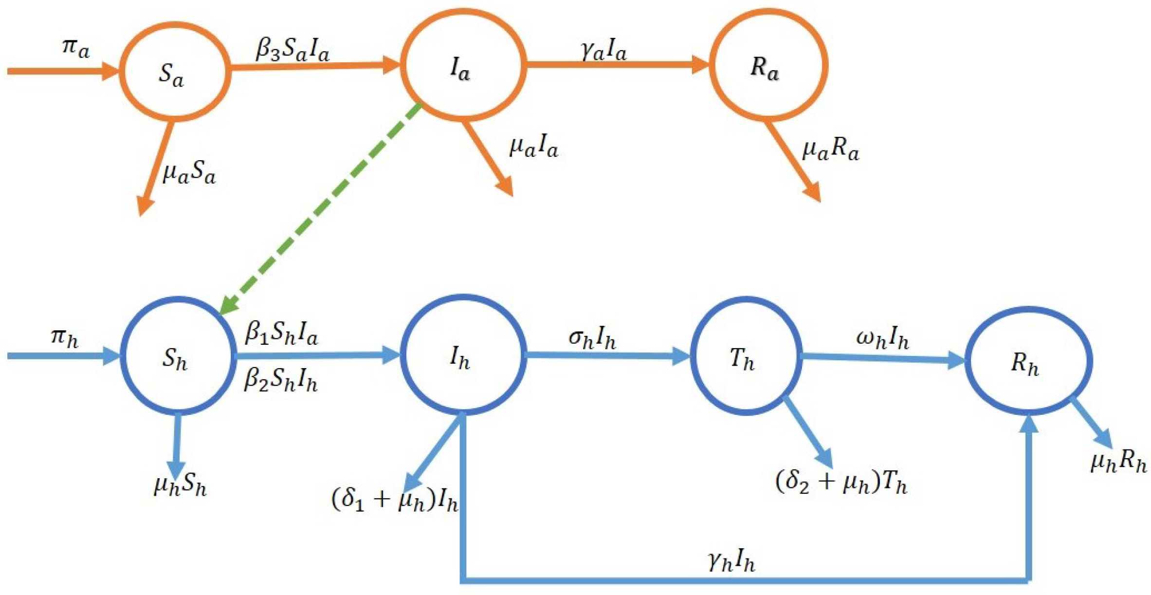
3. A Novel Model Framework for Monkeypox Transmission

The novel model proposes the spread of monkeypox disease between humans and rodents. Unlike existing monkeypox models, treated humans and recovered rodents by natural immunity are considered in the model. Consideration of all possible interactions between two species makes the current model novel. The total human population at time t is represented by $N_h(\aleph )$, susceptible humans $S_h(\aleph )$, infected humans $I_h(\aleph )$, treated humans $T_h(\aleph )$, and recovered humans $R_h(\aleph )$, and $N_h(\aleph )$ = $S_h(\aleph )$ + $I_h(\aleph )$ + $T_h(\aleph )$ + $R_h(\aleph )$. The total population of rodents is $N_a(\aleph )$, susceptible rodents $S_a(\aleph )$, infected rodents $I_a(\aleph )$, and recovered rodents $R_a(\aleph )$ and $N_a(\aleph )$ = $S_a(\aleph )$ + $I_a(\aleph )$ + $R_a(\aleph )$ in Figure 1. Then, the model is built as follows:

$$\begin{array}{cc}\hfill \frac{d{S}_h(\aleph )}{d\aleph }& ={\pi }_h-({\beta }_1{I}_a(\aleph )+{\beta }_2{I}_h(\aleph ))S_h(\aleph )-{\mu }_h{S}_h(\aleph ),\hfill \\ \hfill \frac{d{I}_h(\aleph )}{d\aleph }& =({\beta }_1{I}_a(\aleph )+{\beta }_2{I}_h(\aleph ))S_h(\aleph )-({\gamma }_h+{\sigma }_h+{\mu }_h+{\delta }_1)I_h(\aleph ),\hfill \\ \hfill \frac{d{T}_h(\aleph )}{d\aleph }& ={\sigma }_h{I}_h(\aleph )-({\omega }_h+{\mu }_h+{\delta }_2)T_h(\aleph ),\hfill \\ \hfill \frac{d{R}_h(\aleph )}{d\aleph }& ={\omega }_h{T}_h(\aleph )+{\gamma }_h{I}_h(\aleph )-{\mu }_h{R}_h(\aleph ),\hfill \\ \hfill \frac{d{S}_a(\aleph )}{d\aleph }& ={\pi }_a-{\beta }_3{I}_a(\aleph )S_a(\aleph )-{\mu }_a{S}_a(\aleph ),\hfill \\ \hfill \frac{d{I}_a(\aleph )}{d\aleph }& ={\beta }_3{I}_a(\aleph )S_a(\aleph )-({\gamma }_a+{\mu }_a)I_a(\aleph ),\hfill \\ \hfill \frac{d{R}_a(\aleph )}{d\aleph }& ={\gamma }_a{I}_a(\aleph )-{\mu }_a{R}_a(\aleph ),\hfill \end{array}$$

(3)

We change over the time derivative’s first order on the left side of (3) with the ABC-fractional derivative explained and produce the ABC-fractional derivative model. The following is a possible formulation of the new ABC-fractional model for monkeypox

$$\begin{array}{cc}\hfill {}_0^{ABC}{D}_t^{\rho }\left(S_h(\aleph )\right)& ={\pi }_h-({\beta }_1{I}_a(\aleph )+{\beta }_2{I}_h(\aleph ))S_h(\aleph )-{\mu }_h{S}_h(\aleph ),\hfill \\ \hfill {}_0^{ABC}{D}_t^{\rho }\left(I_h(\aleph )\right)& =({\beta }_1{I}_a(\aleph )+{\beta }_2{I}_h(\aleph ))S_h(\aleph )-({\gamma }_h+{\sigma }_h+{\mu }_h+{\delta }_1)I_h(\aleph ),\hfill \\ \hfill {}_0^{ABC}{D}_t^{\rho }\left(T_h(\aleph )\right)& ={\sigma }_h{I}_h(\aleph )-({\omega }_h+{\mu }_h+{\delta }_2)T_h(\aleph ),\hfill \\ \hfill {}_0^{ABC}{D}_t^{\rho }\left(R_h(\aleph )\right)& ={\omega }_h{T}_h(\aleph )+{\gamma }_h{I}_h(\aleph )-{\mu }_h{R}_h(\aleph ),\hfill \\ \hfill {}_0^{ABC}{D}_t^{\rho }\left(S_a(\aleph )\right)& ={\pi }_a-{\beta }_3{I}_a(\aleph )S_a(\aleph )-{\mu }_a{S}_a(\aleph ),\hfill \\ \hfill {}_0^{ABC}{D}_t^{\rho }\left(I_a(\aleph )\right)& ={\beta }_3{I}_a(\aleph )S_a(\aleph )-({\gamma }_a+{\mu }_a)I_a(\aleph ),\hfill \\ \hfill {}_0^{ABC}{D}_t^{\rho }\left(R_a(\aleph )\right)& ={\gamma }_a{I}_a(\aleph )-{\mu }_a{R}_a(\aleph ),\hfill \end{array}$$

(4)

where the initial conditions are $S_h\left(0\right)=S_{h_0}$, $I_h\left(0\right)=I_{h_0}$, $T_h\left(0\right)=T_{h_0}$, $R_h\left(0\right)=R_{h_0}$, $S_a\left(0\right)=S_{a_0}$, $I_a\left(0\right)=I_{a_0}$, and $R_a\left(0\right)=R_{a_0}$, and the definitions of parameters in the model are listed in

Table 1. Descriptions of the model parameters.

Parameter	Description
${\pi }_h$	The birth rate of humans in the total population
${\beta }_1$	The frequency of virus transmission from infected rats to humans
${\beta }_2$	The frequency of virus transmission to humans from contact with infected humans
${\mu }_h$	Human natural death rate
${\gamma }_h$	Natural rate of human infection recovery
${\sigma }_h$	Human infection treatment rate
${\omega }_h$	The recovery rate of infected humans treated
${\delta }_1$	The death rate of infected humans due to the disease
${\delta }_2$	The death rate of treated humans due to the disease
${\pi }_a$	The birth rate of rodents in the total population
${\beta }_3$	The rate of virus transmission to rodent contact with infected rodent
${\gamma }_a$	Natural recovery rate of infected rodents
${\mu }_a$	Natural death rate of rodents

. Where 0 ≥ t ≥ $t_f$ < ∞, we suppose that

${\zeta }_1(t,S_h(\aleph ),I_h(\aleph ),T_h(\aleph ),R_h(\aleph ),S_a(\aleph ),I_a(\aleph ),R_a(\aleph ))={\pi }_h-({\beta }_1{I}_a(\aleph )+{\beta }_2{I}_h(\aleph ))S_h(\aleph )-$

${\mu }_h{S}_h(\aleph ),$

${\zeta }_2(t,S_h(\aleph ),I_h(\aleph ),T_h(\aleph ),R_h(\aleph ),S_a(\aleph ),I_a(\aleph ),R_a(\aleph ))=({\beta }_1{I}_a(\aleph )+{\beta }_2{I}_h(\aleph ))S_h(\aleph )$

$-({\gamma }_h+{\sigma }_h+{\mu }_h+{\delta }_1)I_h(\aleph ),$

${\zeta }_3(t,S_h(\aleph ),I_h(\aleph ),T_h(\aleph ),R_h(\aleph ),S_a(\aleph ),I_a(\aleph ),R_a(\aleph ))={\sigma }_h{I}_h(\aleph )-({\omega }_h+{\mu }_h+{\delta }_2)T_h(\aleph ),$

${\zeta }_4(t,S_h(\aleph ),I_h(\aleph ),T_h(\aleph ),R_h(\aleph ),S_a(\aleph ),I_a(\aleph ),R_a(\aleph ))={\omega }_h{T}_h(\aleph )+{\gamma }_h{I}_h(\aleph )-{\mu }_h{R}_h(\aleph ),$

${\zeta }_5(t,S_h(\aleph ),I_h(\aleph ),T_h(\aleph ),R_h(\aleph ),S_a(\aleph ),I_a(\aleph ),R_a(\aleph ))={\pi }_a-{\beta }_3{I}_a(\aleph )S_a(\aleph )-{\mu }_a{S}_a(\aleph ),$

${\zeta }_6(t,S_h(\aleph ),I_h(\aleph ),T_h(\aleph ),R_h(\aleph ),S_a(\aleph ),I_a(\aleph ),R_a(\aleph ))={\beta }_3{I}_a(\aleph )S_a(\aleph )-({\gamma }_a+{\mu }_a)I_a(\aleph ),$

${\zeta }_7(t,S_h(\aleph ),I_h(\aleph ),T_h(\aleph ),R_h(\aleph ),S_a(\aleph ),I_a(\aleph ),R_a(\aleph ))={\gamma }_a{I}_a(\aleph )-{\mu }_a{R}_a(\aleph ),$

The above model’s compact form is

$${}_0^{ABC}{D}_t^{\rho }\chi (\aleph )=\zeta (t,\chi (\aleph )),\chi \left(0\right)={\chi }_0\ge 0.$$

Since the given system of differential equation is an autonomous system, it can be written as

$${}_0^{ABC}{D}_t^{\rho }\chi (\aleph )=\zeta \left(\chi (\aleph )\right),\chi \left(0\right)={\chi }_0.$$

where $\chi (\aleph )$ = ${(S_h(\aleph ),I_h(\aleph ),T_h(\aleph ),R_h(\aleph ),S_a(\aleph ),I_a(\aleph ),R_a(\aleph ))}^T\in {\mathbb{R}}^7$ and ${\chi }_0(\aleph )={(S_h\left(0\right),I_h\left(0\right),T_h\left(0\right),R_h\left(0\right),S_a\left(0\right),I_a\left(0\right),R_a\left(0\right))}^T$ is the initial vector.

4. Existence of Solution

The results of the existence analysis for the ABC-fractional order monkeypox transmissible model are discussed in this section.

Definition 1.

Let ϑ be a given function depending on the time and ρ∈ (0,ρ), then, the ρ-order AB integral is characterized as

$${}_0^{AB}{I}_t^{\rho }\varphi (\aleph )=M_1\left(\rho \right)\varphi (\aleph )+M_2\left(\rho \right){\int }_0^t{(t-\vartheta )}^{\rho -1}\varphi \left(\vartheta \right)d\vartheta ,$$

(5)

where $M_1$(ρ) = $\frac{1-\rho }{B\left(\rho \right)}$ and $M_2$(ρ) = $\frac{\rho }{B\left(\rho \right){\Gamma }_{\rho }}$.

Suppose F($\gamma$) is a Banach space of all continuous functions on $\gamma$ = [0,b] and Q = F($\gamma$)X($\gamma$)X($\gamma$)X($\gamma$)X($\gamma$)X($\gamma$)X($\gamma$) with the norm $\left|\right|(S_h,I_h,T_h,R_h,S_a,I_a,R_a)\left|\right|=\left|\right|S_h\left|\right|+\left|\right|I_h\left|\right|+\left|\right|T_h\left|\right|+\left|\right|R_h\left|\right|+\left|\right|S_a\left|\right|+\left|\right|I_a\left|\right|+\left|\right|R_a\left|\right|$, where $\left|\right|S_h\left|\right|=sup\left\{\right|S_h(\aleph )| :t\in \gamma \}$, $\left|\right|I_h\left|\right|=sup\left\{\right|I_h(\aleph )| :t\in \gamma \}$, $\left|\right|T_h\left|\right|=sup\left\{\right|T_h(\aleph )| :t\in \gamma \}$, $\left|\right|R_h\left|\right|=sup\left\{\right|R_h(\aleph )| :t\in \gamma \}$, $\left|\right|S_a\left|\right|=sup\left\{\right|S_a(\aleph )| :t\in \gamma \}$, $\left|\right|I_a\left|\right|=sup\left\{\right|I_a(\aleph )| :t\in \gamma \}$, $\left|\right|R_a\left|\right|=sup\left\{\right|r_a(\aleph )| :t\in \gamma \}$.

Making use of the fractional integral operator as shown in an essential not to be on both sides (4), we obtain

$$\begin{array}{cc}\hfill S_h(\aleph )-S_h\left(0\right)& ={}_0^{AB}{I}_t^{\rho }[{\pi }_h-({\beta }_1{I}_a(\aleph )+{\beta }_2{I}_h(\aleph ))S_h(\aleph )-{\mu }_h{S}_h(\aleph )],\hfill \\ \hfill I_h(\aleph )-I_h\left(0\right)& ={}_0^{AB}{I}_t^{\rho }[({\beta }_1{I}_a(\aleph )+{\beta }_2{I}_h(\aleph ))T_h(\aleph )-({\gamma }_h+{\sigma }_h+{\mu }_h+{\delta }_1)I_h(\aleph )],\hfill \\ \hfill T_h(\aleph )-T_h\left(0\right)& ={}_0^{AB}{I}_t^{\rho }[{\sigma }_h{I}_h(\aleph )-({\omega }_h+{\mu }_h+{\delta }_2)T_h(\aleph )],\hfill \\ \hfill R_h(\aleph )-R_h\left(0\right)& ={}_0^{AB}{I}_t^{\rho }[{\omega }_h{T}_h(\aleph )+{\gamma }_h{I}_h(\aleph )-{\mu }_h{R}_h(\aleph )],\hfill \\ \hfill S_a(\aleph )-S_a\left(0\right)& ={}_0^{AB}{I}_t^{\rho }[{\pi }_a-{\beta }_3{I}_a(\aleph )S_a(\aleph )-{\mu }_a{S}_a(\aleph )],\hfill \\ \hfill I_a(\aleph )-I_a\left(0\right)& ={}_0^{AB}{I}_t^{\rho }[{\beta }_3{I}_a(\aleph )S_a(\aleph )-({\gamma }_a+{\mu }_a)I_a(\aleph )],\hfill \\ \hfill R_a(\aleph )-R_a\left(0\right)& ={}_0^{AB}{I}_t^{\rho }[{\gamma }_a{I}_a(\aleph )-{\mu }_a{R}_a(\aleph )],\hfill \end{array}$$

(6)

By using (5) in (6), we obtain

$$\begin{array}{cc}\hfill S_h(\aleph )-S_h\left(0\right)& =M_1\left(\rho \right)K_1(t,S_h(\aleph ))+M_2\left(\rho \right){}_0{I}^{\rho }{K}_1(t,S_h(\aleph )),\hfill \\ \hfill I_h(\aleph )-I_h\left(0\right)& =M_1\left(\rho \right)K_2(t,I_h(\aleph ))+M_2\left(\rho \right){}_0{I}^{\rho }{K}_2(t,I_h(\aleph )),\hfill \\ \hfill T_h(\aleph )-T_h\left(0\right)& =M_1\left(\rho \right)K_3(t,T_h(\aleph ))+M_2\left(\rho \right){}_0{I}^{\rho }{K}_3(t,T_h(\aleph )),\hfill \\ \hfill R_h(\aleph )-R_h\left(0\right)& =M_1\left(\rho \right)K_4(t,R_h(\aleph ))+M_2\left(\rho \right){}_0{I}^{\rho }{K}_4(t,R_h(\aleph )),\hfill \\ \hfill S_a(\aleph )-S_a\left(0\right)& =M_1\left(\rho \right)K_5(t,S_a(\aleph ))+M_2\left(\rho \right){}_0{I}^{\rho }{K}_5(t,S_a(\aleph )),\hfill \\ \hfill I_a(\aleph )-I_a\left(0\right)& =M_1\left(\rho \right)K_6(t,I_a(\aleph ))+M_2\left(\rho \right){}_0{I}^{\rho }{K}_6(t,I_a(\aleph )),\hfill \\ \hfill R_a(\aleph )-R_a\left(0\right)& =M_1\left(\rho \right)K_7(t,R_a(\aleph ))+M_2\left(\rho \right){}_0{I}^{\rho }{K}_7(t,R_a(\aleph )),\hfill \end{array}$$

(7)

where

$$\begin{array}{cc}\hfill K_1(t,S_h(\aleph ))& ={\pi }_h-({\beta }_1{I}_a(\aleph )+{\beta }_2{I}_h(\aleph ))S_h(\aleph )-{\mu }_h{S}_h(\aleph ),\hfill \\ \hfill K_2(t,I_h(\aleph ))& =({\beta }_1{I}_a(\aleph )+{\beta }_2{I}_h(\aleph ))S_h(\aleph )-({\gamma }_h+{\sigma }_h+{\mu }_h+{\delta }_1)I_h(\aleph ),\hfill \\ \hfill K_3(t,T_h(\aleph ))& ={\sigma }_h{I}_h(\aleph )-({\omega }_h+{\mu }_h+{\delta }_2)T_h(\aleph ),\hfill \\ \hfill K_4(t,R_h(\aleph ))& ={\omega }_h{T}_h(\aleph )+{\gamma }_h{I}_h(\aleph )-{\mu }_h{R}_h(\aleph ),\hfill \\ \hfill K_5(t,S_a(\aleph ))& ={\pi }_a-{\beta }_3{I}_a(\aleph )S_a(\aleph )-{\mu }_a{S}_a(\aleph ),\hfill \\ \hfill K_6(t,I_a(\aleph ))& ={\beta }_3{I}_a(\aleph )S_a(\aleph )-({\gamma }_a+{\mu }_a)I_a(\aleph ),\hfill \\ \hfill K_7(t,R_a(\aleph ))& ={\gamma }_a{I}_a(\aleph )-{\mu }_a{R}_a(\aleph ).\hfill \end{array}$$

(8)

The expression $K_1,K_2,K_3,K_4,K_5,K_6$, and $K_7$ are holds in the Lipschitz criterion iff $S_h,I_h,T_h,R_h,S_a,I_a,$ and $R_a$ has an upper bound.

If we assume that there are two functions, $S_h(\aleph )$ and $S_h^{*}(\aleph )$, we have

$$\begin{array}{ccc}\hfill \left|\right|K-1(t,S_h(\aleph ))-K_1(t,S_h^{*}(\aleph ))\left|\right|=\left|\right|{\pi }_h-({\beta }_1{I}_a(\aleph )& +\hfill & {\beta }_2{I}_h(S_h(\aleph )-S_h^{*}(\aleph )))\hfill \\ \hfill & -\hfill & {\mu }_h(S_h(\aleph )-S_h^{*}(\aleph ))\left|\right|\hfill \end{array}$$

(9)

Considering ${\eta }_1$ = $\left|\right|({\beta }_1{I}_a(\aleph )+{\beta }_2{I}_h+{\mu }_h||$ and $I_a,I_h$ is a bounded function, then we obtain

$$\left|\right|K_1(t,S_h(\aleph ))-K_1(t,S_h^{*}(\aleph ))\left|\right|\le {\eta }_1\left|\right|S_h(\aleph )-S_h^{*}(\aleph )\left|\right|,$$

(10)

With the similar procedure, the result deduced to

$$\begin{array}{c}\left|\right|K_2(t,I_h(\aleph ))-K_2(t,I_h^{*}(\aleph ))\left|\right|\le {\eta }_2\left|\right|I_h(\aleph )-I_h^{*}(\aleph )\left|\right|,\\ \left|\right|K_3(t,T_h(\aleph ))-K_3(t,T_h^{*}(\aleph ))\left|\right|\le {\eta }_3\left|\right|T_h(\aleph )-T_h^{*}(\aleph )\left|\right|,\\ \left|\right|K_4(t,R_h(\aleph ))-K_4(t,R_h^{*}(\aleph ))\left|\right|\le {\eta }_4\left|\right|R_h(\aleph )-R_h^{*}(\aleph )\left|\right|,\\ \left|\right|K_5(t,S_a(\aleph ))-K_5(t,S_a^{*}(\aleph ))\left|\right|\le {\eta }_5\left|\right|S_a(\aleph )-S_a^{*}(\aleph )\left|\right|,\\ \left|\right|K_6(t,I_a(\aleph ))-K_6(t,I_a^{*}(\aleph ))\left|\right|\le {\eta }_6\left|\right|I_a(\aleph )-I_a^{*}(\aleph )\left|\right|,\\ \left|\right|K_7(t,R_a(\aleph ))-K_7(t,R_a^{*}(\aleph ))\left|\right|\le {\eta }_7\left|\right|R_a(\aleph )-R_a^{*}(\aleph )\left|\right|,\end{array}$$

(11)

Hence, all the seven functions $K_1, K_2, K_3, K_4, K_5, K_6,$ and $K_7$ hold the Lipschitz criterion. Recursively, the expression in (7) can be written as

$$\begin{array}{c}{S}_{h_n}(\aleph )=M_1\left(\rho \right)K_1(t,S_{h_{n-1}}(\aleph ))+M_2\left(\rho \right){}_0{I}^{\rho }{K}_1(t,S_{h_{n-1}}(\aleph )),\\ I_{h_n}(\aleph )=M_1\left(\rho \right)K_2(t,I_{h_{n-1}}(\aleph ))+M_2\left(\rho \right){}_0{I}^{\rho }{K}_2(t,T_{h_{n-1}}(\aleph )),\\ T_{h_n}(\aleph )=M_1\left(\rho \right)K_3(t,T_{h_{n-1}}(\aleph ))+M_2\left(\rho \right){}_0{I}^{\rho }{K}_3(t,T_{h_{n-1}}(\aleph )),\\ R_{h_n}(\aleph )=M_1\left(\rho \right)K_4(t,R_{h_{n-1}}(\aleph ))+M_2\left(\rho \right){}_0{I}^{\rho }{K}_4(t,R_{h_{n-1}}(\aleph )),\\ S_{a_n}(\aleph )=M_1\left(\rho \right)K_5(t,S_{a_{n-1}}(\aleph ))+M_2\left(\rho \right){}_0{I}^{\rho }{K}_5(t,S_{a_{n-1}}(\aleph )),\\ I_{a_n}(\aleph )=M_1\left(\rho \right)K_6(t,I_{a_{n-1}}(\aleph ))+M_2\left(\rho \right){}_0{I}^{\rho }{K}_6(t,I_{a_{n-1}}(\aleph )),\\ R_{a_n}(\aleph )=M_1\left(\rho \right)K_7(t,R_{a_{n-1}}(\aleph ))+M_2\left(\rho \right){}_0{I}^{\rho }{K}_7(t,R_{a_{n-1}}(\aleph )).\end{array}$$

(12)

along with the initial starting point $S_{h_0}(\aleph )=S_h\left(0\right)$, $I_{h_0}(\aleph )=I_h\left(0\right)$, $T_{h_0}(\aleph )=T_h\left(0\right)$, $R_{h_0}(\aleph )=R_h\left(0\right)$, $S_{a_0}(\aleph )=S_a\left(0\right)$, $I_{a_0}(\aleph )=I_a\left(0\right)$, and $R_{a_0}(\aleph )=R_a\left(0\right)$. By computing the difference between the succeeding terms, the following was determined.

$$\begin{array}{cc}\hfill \psi S_{h_n}=S_{h_n}(\aleph )-S_{h_{n-1}}(\aleph )& =M_1\left(\rho \right)[K_1(t,S_{h_{n-1}})-K_1(t,S_{h_{n-2}})]\hfill \\ \hfill +& M_2{}_0{I}^{\rho }[K_1(t,S_{h_{n-1}})-K_1(t,S_{h_{n-2}})],\hfill \\ \hfill \psi I_{h_n}=I_{h_n}(\aleph )-I_{h_{n-1}}(\aleph )& =M_1\left(\rho \right)[K_2(t,I_{h_{n-1}})-K_2(t,I_{h_{n-2}})]\hfill \\ \hfill +& M_2{}_0{I}^{\rho }[K_2(t,I_{h_{n-1}})-K_2(t,I_{h_{n-2}})],\hfill \\ \hfill \psi T_{h_n}=T_{h_n}(\aleph )-T_{h_{n-1}}(\aleph )& =M_1\left(\rho \right)[K_3(t,T_{h_{n-1}})-K_3(t,T_{h_{n-2}})]\hfill \\ \hfill +& M_2{}_0{I}^{\rho }[K_3(t,T_{h_{n-1}})-K_3(t,S_{h_{n-2}})],\hfill \\ \hfill \psi R_{h_n}=R_{h_n}(\aleph )-R_{h_{n-1}}(\aleph )& =M_1\left(\rho \right)[K_4(t,R_{h_{n-1}})-K_4(t,T_{h_{n-2}})]\hfill \\ \hfill +& M_2{}_0{I}^{\rho }[K_4(t,R_{h_{n-1}})-K_4(t,R_{h_{n-2}})],\hfill \\ \hfill \psi S_{a_n}=S_{a_n}(\aleph )-S_{a_{n-1}}(\aleph )& =M_1\left(\rho \right)[K_5(t,S_{a_{n-1}})-K_5(t,S_{a_{n-2}})]\hfill \\ \hfill +& M_2{}_0{I}^{\rho }[K_5(t,S_{a_{n-1}})-K_5(t,S_{a_{n-2}})],\hfill \\ \hfill \psi I_{a_n}=I_{a_n}(\aleph )-I_{a_{n-1}}(\aleph )& =M_1\left(\rho \right)[K_6(t,I_{a_{n-1}})-K_6(t,I_{a_{n-2}})]\hfill \\ \hfill +& M_2{}_0{I}^{\rho }[K_6(t,I_{h_{n-1}})-K_6(t,I_{h_{n-2}})],\hfill \\ \hfill \psi R_{a_n}=R_{a_n}(\aleph )-R_{a_{n-1}}(\aleph )& =M_1\left(\rho \right)[K_7(t,R_{a_{n-1}})-K_7(t,R_{a_{n-2}})]\hfill \\ \hfill +& M_2{}_0{I}^{\rho }[K_7(t,R_{a_{n-1}})-K_7(t,R_{a_{n-2}})].\hfill \end{array}$$

(13)

It is critical to note that

$$\begin{array}{cc}\hfill & S_{h_n}(\aleph )=\sum _{i=0}^n\psi S_{h_i}(\aleph ),I_{h_n}(\aleph )=\sum _{i=0}^n\psi I_{h_i}(\aleph ),T_{h_n}(\aleph )=\sum _{i=0}^n\psi T_{h_i}(\aleph ),R_{h_n}(\aleph )=\sum _{i=0}^n\psi R_{h_i}(\aleph ),\hfill \\ \hfill & S_{a_n}(\aleph )=\sum _{i=0}^n\psi S_{a,i}(\aleph ),I_{a_n}(\aleph )=\sum _{i=0}^n\psi I_{a_i}(\aleph ),R_{a_n}(\aleph )=\sum _{i=0}^n\psi R_{a_i}(\aleph ).\hfill \end{array}$$

Additionally, utilizing (12) and considering that

$$\begin{array}{cc}\hfill & \psi S_{h_n}(\aleph )=S_{h_{n-1}}(\aleph )-S_{h_{n-2}}(\aleph ),\psi I_{h_n}(\aleph )=I_{h_{n-1}}(\aleph )-I_{h_{n-2}}(\aleph ),\hfill \\ \hfill & \psi T_{h_n}(\aleph )=T_{h_{n-1}}(\aleph )-T_{h_{n-2}}(\aleph ),\psi R_{h_n}(\aleph )=R_{h_{n-1}}(\aleph )-R_{h_{n-2}}(\aleph ),\hfill \\ \hfill & \psi S_{a_n}(\aleph )=S_{a_{n-1}}(\aleph )-S_{a_{n-2}}(\aleph ),\psi I_{a_n}(\aleph )=I_{a_{n-1}}(\aleph )-I_{a_{n-2}}(\aleph ),\hfill \\ \hfill & \psi R_{a_n}(\aleph )=R_{a_{n-1}}(\aleph )-R_{a_{n-2}}(\aleph ),\hfill \end{array}$$

we derive

$$\begin{array}{cc}\hfill \left|\right|\psi S_{h_n}(\aleph )\left|\right|& =M_1\left(\rho \right){\eta }_1\left|\right|\psi S_{h_{n-1}}(\aleph )\left|\right|+M_2\left(\rho \right){\eta }_1{}_0{I}^{\rho }\left|\right|S_{h_{n-1}}(\aleph )\left|\right|,\hfill \\ \hfill \left|\right|\psi I_{h_n}(\aleph )\left|\right|& =M_1\left(\rho \right){\eta }_1\left|\right|\psi I_{h_{n-1}}(\aleph )\left|\right|+M_2\left(\rho \right){\eta }_1{}_0{I}^{\rho }\left|\right|I_{h_{n-1}}(\aleph )\left|\right|,\hfill \\ \hfill \left|\right|\psi T_{h_n}(\aleph )\left|\right|& =M_1\left(\rho \right){\eta }_1\left|\right|\psi T_{h_{n-1}}(\aleph )\left|\right|+M_2\left(\rho \right){\eta }_1{}_0{I}^{\rho }\left|\right|T_{h_{n-1}}(\aleph )\left|\right|,\hfill \\ \hfill \left|\right|\psi R_{h_n}(\aleph )\left|\right|& =M_1\left(\rho \right){\eta }_1\left|\right|\psi R_{h_{n-1}}(\aleph )\left|\right|+M_2\left(\rho \right){\eta }_1{}_0{I}^{\rho }\left|\right|R_{h_{n-1}}(\aleph )\left|\right|,\hfill \\ \hfill \left|\right|\psi S_{a_n}(\aleph )\left|\right|& =M_1\left(\rho \right){\eta }_1\left|\right|\psi S_{a_{n-1}}(\aleph )\left|\right|+M_2\left(\rho \right){\eta }_1{}_0{I}^{\rho }\left|\right|S_{a_{n-1}}(\aleph )\left|\right|,\hfill \\ \hfill \left|\right|\psi I_{a_n}(\aleph )\left|\right|& =M_1\left(\rho \right){\eta }_1\left|\right|\psi I_{a_{n-1}}(\aleph )\left|\right|+M_2\left(\rho \right){\eta }_1{}_0{I}^{\rho }\left|\right|I_{a_{n-1}}(\aleph )\left|\right|,\hfill \\ \hfill \left|\right|\psi R_{a_n}(\aleph )\left|\right|& =M_1\left(\rho \right){\eta }_1\left|\right|\psi R_{a_{n-1}}(\aleph )\left|\right|+M_2\left(\rho \right){\eta }_1{}_0{I}^{\rho }\left|\right|R_{a_{n-1}}(\aleph )\left|\right|.\hfill \end{array}$$

(14)

Theorem 4.

Let the following condition be satisfied,

$$M_1\left(\rho \right){\eta }_i+\frac{M_2\left(\rho \right)}{\rho }{(\aleph )}^{\rho }{\eta }_i\le 1,i=1,2,\dots ,7$$

(15)

Therefore, t ∈ [0,1] provides a unique solution for the fractional epidemic model (4).

Proof. 

It is clear that the functions $S_h(\aleph ),I_h(\aleph ),T_h(\aleph ),R_h(\aleph ),S_a(\aleph ),I_a(\aleph ),$ and $R_a(\aleph )$ are bounded. The expressions $K_1, K_2, K_3, K_4, K_5, K_6$, and $K_7$ hold the Lipschitz criterion. Therefore, using (14) and a recursive principle, the following concluded.

$$\begin{array}{cc}\hfill \left|\right|\psi S_{h_n}(\aleph )\left|\right|& \le \left|\right|S_{h_0}(\aleph ){\left(M_1\left(\rho \right){\eta }_1+\frac{M_2\left(\rho \right)}{\rho }{(\aleph )}^{\rho }{\eta }_1\right)}^n,\hfill \\ \hfill \left|\right|\psi I_{h_n}(\aleph )\left|\right|& \le \left|\right|I_{h_0}(\aleph ){\left(M_1\left(\rho \right){\eta }_2+\frac{M_2\left(\rho \right)}{\rho }{(\aleph )}^{\rho }{\eta }_2\right)}^n,\hfill \\ \hfill \left|\right|\psi T_{h_n}(\aleph )\left|\right|& \le \left|\right|T_{h_0}(\aleph ){\left(M_1\left(\rho \right){\eta }_3+\frac{M_2\left(\rho \right)}{\rho }{(\aleph )}^{\rho }{\eta }_3\right)}^n,\hfill \\ \hfill \left|\right|\psi R_{h_n}(\aleph )\left|\right|& \le \left|\right|R_{h_0}(\aleph ){\left(M_1\left(\rho \right){\eta }_4+\frac{M_2\left(\rho \right)}{\rho }{(\aleph )}^{\rho }{\eta }_4\right)}^n,\hfill \\ \hfill \left|\right|\psi S_{a_n}(\aleph )\left|\right|& \le \left|\right|S_{a_0}(\aleph ){\left(M_1\left(\rho \right){\eta }_5+\frac{M_2\left(\rho \right)}{\rho }{(\aleph )}^{\rho }{\eta }_5\right)}^n,\hfill \\ \hfill \left|\right|\psi I_{a_n}(\aleph )\left|\right|& \le \left|\right|I_{a_0}(\aleph ){\left(M_1\left(\rho \right){\eta }_6+\frac{M_2\left(\rho \right)}{\rho }{(\aleph )}^{\rho }{\eta }_6\right)}^n,\hfill \\ \hfill \left|\right|\psi R_{a_n}(\aleph )\left|\right|& \le \left|\right|R_{a_0}(\aleph ){\left(M_1\left(\rho \right){\eta }_7+\frac{M_2\left(\rho \right)}{\rho }{(\aleph )}^{\rho }{\eta }_7\right)}^n.\hfill \end{array}$$

(16)

Therefore, it implies for n $\to \infty$, all mapping exists and fulfill $\left|\right|\psi S_{h_n}(\aleph )\left|\right|\to 0,$ $\left|\right|\psi I_{h_n}(\aleph )\left|\right|\to 0,$ $\left|\right|\psi T_{h_n}(\aleph )\left|\right|\to 0,$ $\left|\right|\psi R_{h_n}(\aleph )\left|\right|\to 0,$ $\left|\right|\psi S_{a_n}(\aleph )\left|\right|\to 0,$ $\left|\right|\psi I_{a_n}(\aleph )\left|\right|\to 0,$ $\left|\right|\psi R_{a_n}(\aleph )\left|\right|\to 0.$ Now, using the triangle inequality of (12), we obtain for every k

$$\begin{array}{c}\hfill \left|\right|S_{h_{n+k}}(\aleph )-S_{h_n}(\aleph )\left|\right|\le \sum _{j=n+1}^{n+k}{r}_1^j=\frac{r_1^{n+1}-r_1^{n+k+1}}{1-r_1},\\ \hfill \left|\right|I_{h_{n+k}}(\aleph )-I_{h_n}(\aleph )\left|\right|\le \sum _{j=n+1}^{n+k}{r}_2^j=\frac{r_2^{n+1}-r_2^{n+k+1}}{1-r_2},\\ \hfill \left|\right|T_{h_{n+k}}(\aleph )-T_{h_n}(\aleph )\left|\right|\le \sum _{j=n+1}^{n+k}{r}_3^j=\frac{r_3^{n+1}-r_3^{n+k+1}}{1-r_3},\\ \hfill \left|\right|R_{h_{n+k}}(\aleph )-R_{h_n}(\aleph )\left|\right|\le \sum _{j=n+1}^{n+k}{r}_4^j=\frac{r_4^{n+1}-r_4^{n+k+1}}{1-r_4},\\ \hfill \left|\right|S_{a_{n+k}}(\aleph )-S_{a_n}(\aleph )\left|\right|\le \sum _{j=n+1}^{n+k}{r}_5^j=\frac{r_5^{n+1}-r_5^{n+k+1}}{1-r_5},\\ \hfill \left|\right|I_{a_{n+k}}(\aleph )-I_{a_n}(\aleph )\left|\right|\le \sum _{j=n+1}^{n+k}{r}_6^j=\frac{r_6^{n+1}-r_6^{n+k+1}}{1-r_6},\\ \hfill \left|\right|R_{a_{n+k}}(\aleph )-R_{a_n}(\aleph )\left|\right|\le \sum _{j=n+1}^{n+k}{r}_7^j=\frac{r_7^{n+1}-r_7^{n+k+1}}{1-r_7},\end{array}$$

(17)

where $r_i=M_1\left(\rho \right){\eta }_i+\frac{M_2\left(\rho \right)}{\rho }{(\aleph )}^{\rho }{\eta }_i\le 1$ by assumption. Hence $S_h(\aleph ),I_h(\aleph ),T_h(\aleph ),R_h(\aleph ),S_a(\aleph ),I_a(\aleph ),$ and $R_a(\aleph )$ are utilizing the concept of the limit in Equation (12) as n → ∞, Cauchy sequences and uniformly convergent in the Banach spaces C$\left(\gamma \right)$, for evidence that the limit of these sequences has a unique solution to the fractional derivative Equation (4), see [57].

This shows that the solution of Equation (4) exists and satisfies all the conditions (15). □

5. Equilibrium Points

Now, let us determine the equilibrium points in order to analyze the stability of the system. One of them is the monkeypox-free equilibrium point. Monkeypox-free equilibrium is the case of no disease among humans and rodents, namely, where the infected human populations are equal to zero. Thus, the MFE point of the system (4) is given by

$$E^0=(S_h^0,I_h^0,T_h^0,R_h^0,S_a^0,I_a^0,R_a^0)=\left(\frac{{\pi }_h}{{\mu }_h},0,0,0,\frac{{\pi }_a}{{\mu }_a},0,0\right)$$

(18)

Endemic equilibrium point of the fractional order model (4), denoted by $E^0$, is obtained by considering ${}_0^{ABC}{D}_t^{\rho }{\chi }_i(\aleph )$ = 0 for each state variable ${\chi }_i$, i = 1, 2, …, 7 and by solving the resultant equations to produce the following (see [57]);

$$E^{*}=(S_h^{*},I_h^{*},T_h^{*},R_h^{*},S_a^{*},I_a^{*},R_a^{*})$$

where

$$\begin{array}{cc}\hfill S_h^{*}& =\frac{{\pi }_h}{({\beta }_1{I}_a^{*}+{\beta }_2^{*}+{\mu }_h)},I_h^{*}=\frac{({\beta }_1{I}_a^{*}+{\beta }_2{I}_h^{*})S^{*}}{({\mu }_h+{\sigma }_h+{\gamma }_h+{\delta }_1)},\hfill \\ \hfill T_h^{*}& =\frac{\left({\sigma }_h{I}_h^{*}\right)}{({\mu }_h+{\omega }_h+{\delta }_2)},R_h^{*}=\frac{({\omega }_h{T}_h^{*}+{\gamma }_h{I}_h^{*})}{\left({\mu }_h\right)},\hfill \\ \hfill S_a^{*}& =\frac{{\pi }_a}{({\beta }_3{I}_a^{*}+{\mu }_a)},I_a^{*}=\frac{\left({\beta }_3{I}_a^{*}\right)}{({\gamma }_a+{\mu }_a)},R_a^{*}=\frac{{\gamma }_a{I}_a^{*}}{{\mu }_a}.\hfill \end{array}$$

The endemic equilibrium point is given by using the next-generation matrix [22,57], the basic $\left(R_0\right)$ of $R_0$

$$R_o=\frac{{\beta }_2{\pi }_h}{{\mu }_h({\gamma }_h+{\sigma }_h+{\mu }_h+{\delta }_1)}$$

(19)

If $R_0<1$, monkeypox has lost its effect in the population and the virus is eradicated from the population. If $R_0>1$, the number of infectious people is constantly increasing because the infection is present, and the disruptive impact of monkeypox on the population persists.

6. Stability Analysis

In this section, the stability of equilibrium points is investigated. The system (4) is a Jacobian matrix.

Theorem 5.

The monkeypox equilibrium point $E^0$ is locally asymptotically stable if the condition

$$R_0\le 1and{\beta }_3\frac{{\pi }_a}{{\mu }_a}\le {\gamma }_a+{\mu }_a,$$

is provided. It is unstable otherwise.

Proof. 

The Jacobian matrix of system (4) at $E^0$ is (see [22,57])

$$J\left(E^0\right)=\left[\begin{array}{cccccccc}& -{\mu }_h& -{\beta }_2\frac{{\pi }_h}{{\mu }_h}& 0& 0& 0& -{\beta }_1\frac{{\pi }_h}{{\mu }_h}& 0\\ & 0& d_1& 0& 0& 0& {\beta }_1\frac{{\pi }_h}{{\mu }_h}& 0\\ & 0& {\sigma }_h& d_2& 0& 0& 0& 0\\ & 0& {\gamma }_h& {\omega }_h& -{\mu }_h& 0& 0& 0\\ & 0& 0& 0& 0& -{\mu }_h& -{\beta }_3\frac{{\pi }_a}{{\mu }_a}& 0\\ & 0& -{\beta }_1\frac{{\pi }_h}{{\mu }_h}& 0& 0& 0& d_3& 0\\ & 0& {\beta }_1\frac{{\pi }_h}{{\mu }_h}& 0& 0& 0& {\gamma }_a& -{\mu }_a\end{array}\right]$$

(20)

where $d_1={\beta }_2\frac{{\pi }_h}{{\mu }_h}-({\gamma }_h+{\sigma }_h+{\mu }_h+{\delta }_1)$, $d_2=-({\omega }_h+{\mu }_h+{\delta }_2)$, $d_3={\beta }_3\frac{{\pi }_a}{{\mu }_a}-({\gamma }_a+{\mu }_a)$. The negative eigenvalues of this matrix are ${\lambda }_{1,2}=-{\mu }_h, {\lambda }_3=-({\omega }_h+{\mu }_h+{\delta }_2), {\lambda }_{4,5}=-{\mu }_a$. Other eigenvalues are ${\lambda }_6={\beta }_2\frac{{\pi }_h}{{\mu }_h}-({\gamma }_h+{\sigma }_h+{\mu }_h+{\delta }_1)=({\gamma }_h+{\sigma }_h+{\mu }_h+{\delta }_1)(R_0-1)$, and ${\lambda }_7={\beta }_3\frac{{\pi }_h}{{\mu }_a}-({\gamma }_a+{\mu }_a).$

If $R_0\le 1$ and ${\beta }_3\frac{{\pi }_a}{{\mu }_a}\le {\gamma }_a+{\mu }_a$, the system (4) is locally asymptotically stable at point $E^0$. However, if $R_0>1$ and ${\beta }_3\frac{{\pi }_a}{{\mu }_a}>({\gamma }_a+{\mu }_a)$, the system (4) is unstable at point $E^0$, and there is a point $E^{*}$ where the system is stable. □

Theorem 6.

If $R_0>1$, the system (4) is locally asymptotically stable at endemic equilibrim point $E^{*}$.

Proof. 

[22,57] The Jacobian matrix of system (4) at $E^{*}$

$$J\left(E^{*}\right)=\left[\begin{array}{cccccccc}& -a_1-{\mu }_h& -{\beta }_2{S}_h^{*}& 0& 0& 0& -{\beta }_1{S}_h^{*}& 0\\ & a_1& a_2& 0& 0& 0& {\beta }_1{S}_h^{*}& 0\\ & 0& {\sigma }_h& a_3& 0& 0& 0& 0\\ & 0& {\gamma }_h& {\omega }_h& -{\mu }_h& 0& 0& 0\\ & 0& 0& 0& 0& -{\beta }_3{I}_a^{*}-{\mu }_a& -{\beta }_3{S}_a^{*}& 0\\ & 0& -{\beta }_1{S}_h^{*}& 0& 0& {\beta }_3{I}_a^{*}& a_4& 0\\ & 0& {\beta }_1{S}_h^{*}& 0& 0& 0& {\gamma }_a& -{\mu }_a\end{array}\right]$$

(21)

where $a_1={\beta }_1{I}_a^{*}+{\beta }_2{I}_h^{*}, a_2={\beta }_2{S}_h^{*}-({\gamma }_h+{\sigma }_h+{\mu }_h+{\delta }_1), a_3=-({\omega }_h+{\mu }_h+{\delta }_2), a_4={\beta }_3{S}_a^{*}-({\gamma }_a+{\mu }_a)$. The negative eigenvalues are ${\chi }_1=-{\mu }_h, {\chi }_2=-({\omega }_h+{\mu }_h+{\delta }_2), {\chi }_3=-{\mu }_a, {\chi }_4=-({\beta }_1{I}_a^{*}+{\beta }_2{I}_h^{*})-{\mu }_h$, and ${\chi }_5=-{\beta }_3{I}_a^{*}-{\mu }_a$.

The following characteristic equation gives the other eigenvalues:

$${\chi }^2+b_1\chi +b_2=0$$

(22)

in which the coefficients are $b_1={\delta }_1+{\gamma }_a+{\gamma }_h+{\mu }_a+{\mu }_h-{\beta }_3{S}_a^{*}-{\beta }_2{S}_h^{*}+{\sigma }_h,$ $b_2={\beta }_1{S}_h^{*}\left({\beta }_1{S}_h^{*}{\beta }_2{I}_a^{*}\right)+{\beta }_2{S}_h^{*}(-{\gamma }_a+{\beta }_2{I}_h^{*}-{\mu }_a+{\beta }_3{S}_a^{*})-S_a^{*}({\delta }_1+{\gamma }_h-{\beta }_3{I}_a^{*}-{\mu }_h)+{\gamma }_a({\delta }_1+{\gamma }_h+{\mu }_a+{\mu }_h)+{\mu }_a({\delta }_1+{\mu }_h)+{\sigma }_h({\gamma }_a+{\mu }_a-S_a^{*})$.

If the coefficients $b_1$ and $b_2$ of the characteristic Equation (22) provides the conditions $b_1,b_2>0,$ or $b_1<0,4b_2>{\left(b_1\right)}^2$, there are two negative eigenvalues. From the Routh–Hurwitz criteria, the system (4) is locally asymptotic at point $E^{*}$. □

Numerical Results

In this section, the optimal system given by (4) is numerically solved using the FDE 12 in MATLAB 2018. This graphs the stability of equilibrium points; the critical periods for when preventive and therapeutic control strategies for a viral disease become particularly important are the periods when the spread of the virus accelerates and turns into an epidemic. Epidemiologically, this corresponds to $R_0>1$. Therefore, $R_o=3.5$ is the value considered, and the corresponding system parameters, the dynamic system (27), and initial condition $S_h\left(0\right)=0.90$, $I_h\left(0\right)=0.20$, $T_h\left(0\right)=0$, $R_h\left(0\right)=0$, $S_a\left(0\right)=0.90$, $I_a\left(0\right)=0.07$, $R_a\left(0\right)=$ Also, the data for the parameters are used to determine the value for, see [14,18], ${\pi }_h=0.029,$ ${\pi }_a=2.0,$ ${\beta }_1=0.00025,$ ${\beta }_2=0.00006,$ ${\beta }_3=0.027,$ ${\mu }_h=0.02,$ ${\mu }_a=1.5,$ ${\gamma }_h=1/21,$ ${\gamma }_a=0.6,$ ${\sigma }_h=0.00025,$ ${\delta }_1=0.1,$ ${\delta }_2=0.4,$ ${\omega }_h=0.004$, and the fractional order $\rho$ ∈ [0,1].

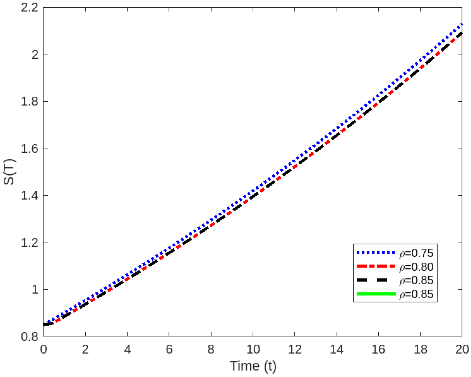
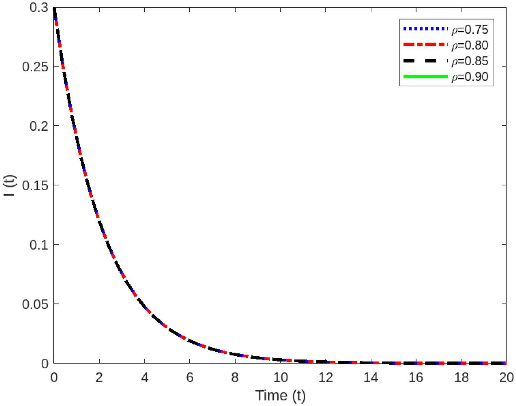
This Figure 2, Figure 3, Figure 4 and Figure 5 show that the number of susceptible individuals is quickly reducing, and that these people are quickly infected. Because of the nature of the condition, this is a predicted outcome. While some infected persons recover with treatment, most people are cured naturally, with a recovery rate of about 0.80.

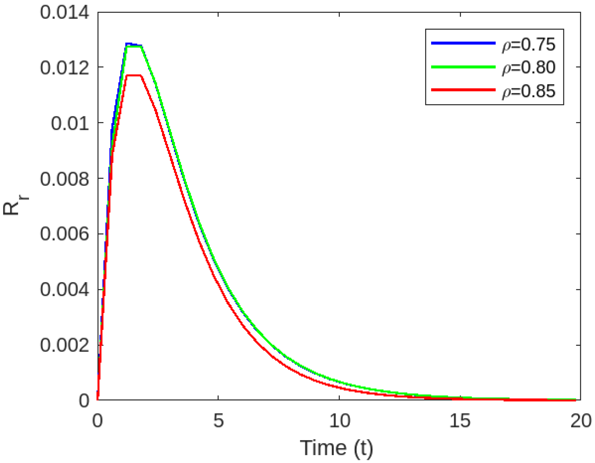
This Figure 6, Figure 7 and Figure 8 depending on the transmission rate in rodents, the rate of susceptible rodents decreased and the infected rodents entered the recovered compartment. However, since the death rate of rodents is lower, the rate of recovered rodents approaches 0.30.

7. Optimal Control Analysis

Unfortunately, this disease is significantly affecting public health, especially in West and Central African countries with low levels of development. Its influence still continues in many areas. For this reason, optimal preventive and treatment measures that can control the spread of the disease have gained importance. In this context, our symmetry model is described as an optimal control problem by adapting optimal treatment strategies. Although the vaccine is the most effective method against viral diseases, it has difficulties such as continuous progress and supply according to the structure of the virus. Therefore, as a natural consequence of sensitivity analysis, it is aimed to reduce the rate of human-to-human transmission represented by the parameter ${\beta }_2$. Thus, some of the ways to dampen the spread of monkeypox virus are preventive measures such as mask usage, social distance, hygiene, etc. In addition, it is necessary to increase the rate of treatment of infected people, represented by the parametrized ${\sigma }_h$, to further slow down the spread of the pandemic. The strategies mentioned for a novel monkeypox model developed in this study are adapted to the symmetry model as control variables to prevent spread. The goal of optimal control problem is to minimize the following objective functional:

$$J(u_1,u_2)=min{\int }_0^T\left[I_h(\aleph )+\frac{1}{2}(K_1{u}_1^2(\aleph )+K_2{u}_2^2(\aleph ))\right]dt.$$

(23)

Model (4) is changed to model (23), and subject to the state system, through incorporating the control variable.

$$\begin{array}{ccc}\hfill {}_0^{ABC}{D}_t^{\rho }\left(S_h(\aleph )\right)& =& {\pi }_h-(1-u_1(\aleph ))({\beta }_1{I}_a(\aleph )+{\beta }_2{I}_h(\aleph ))S_h(\aleph )-{\mu }_h{S}_h(\aleph ),\hfill \\ \hfill {}_0^{ABC}{D}_t^{\rho }\left(I_h(\aleph )\right)& =& (1-u_1(\aleph ))({\beta }_1{I}_a(\aleph )+{\beta }_2{I}_h(\aleph ))S_h(\aleph )-({\gamma }_h+u_2+{\mu }_h+{\delta }_1)I_h(\aleph ),\hfill \\ \hfill {}_0^{ABC}{D}_t^{\rho }\left(T_h(\aleph )\right)& =& u_2(\aleph )I_h(\aleph )-({\omega }_h+{\mu }_h+{\delta }_2)T_h(\aleph ),\hfill \\ \hfill {}_0^{ABC}{D}_t^{\rho }\left(R_h(\aleph )\right)& =& {\omega }_h{T}_h(\aleph )+{\gamma }_h{I}_h(\aleph )-{\mu }_h{R}_h(\aleph ),\hfill \\ \hfill {}_0^{ABC}{D}_t^{\rho }\left(S_a(\aleph )\right)& =& {\pi }_a-{\beta }_3{I}_a(\aleph )S_a(\aleph )-{\mu }_a{S}_a(\aleph ),\hfill \\ \hfill {}_0^{ABC}{D}_t^{\rho }\left(I_a(\aleph )\right)& =& {\beta }_3{I}_a(\aleph )S_a(\aleph )-({\gamma }_a+{\mu }_a)I_a(\aleph ),\hfill \\ \hfill {}_0^{ABC}{D}_t^{\rho }\left(R_a(\aleph )\right)& =& {\gamma }_a{I}_a(\aleph )-{\mu }_a{R}_a(\aleph ),\hfill \end{array}$$

(24)

with initial conditions

$S_h\left(0\right)\ge 0,I_h\left(0\right)\ge 0,T_h\left(0\right)\ge 0,R_h\left(0\right)\ge 0,$$S_a\left(0\right)\ge 0,I_a\left(0\right)\ge 0,R_a\left(0\right)\ge 0.$

We use two control variables, i.e., where $u_1(\aleph )$ stands for prevention such as mask usage, social distancing, and hygiene, and ${\sigma }_h$ is considered as the control variable $u_2(\aleph )$ to determine the optimal treatment strategy that represents the optimal rate of treatment required for infected humans.

$I_h$ are relative weights in the objective function (23), whereas $K_1$ and $K_2$ measure the costs related to social distance and treatment, respectively. Our objective is to locate the controlling function so that

$$J(u_1^{*},u_2^{*})=min\{J(u_1,u_2),u_1,u_2\in U\}.$$

(25)

In terms of the system (24), the control set is described as

$$U=\{(u_1,u_2)/u_i(\aleph )\le ,i=1,2\}.$$

(26)

By applying Pontryagin’s maximum principle, the requirements that an optimal solution must satisfy are discovered. This principle transforms Equations (23) and (24) into a problem where the Hamiltonian H is minimized with regard to the control variables:

$$\begin{array}{cc}\hfill H=& I_h(\aleph )+\frac{1}{2}(K_1{u}_1^2(\aleph )+K_2{u}_2^2(\aleph ))\hfill \\ \hfill & +{\lambda }_1(\aleph )[{\pi }_h-(1-u_1(\aleph ))({\beta }_1{I}_a(\aleph )+{\beta }_2{I}_h(\aleph ))S_h(\aleph )-{\mu }_h{S}_h(\aleph )],\hfill \\ \hfill & +{\lambda }_2(\aleph )[(1-u_1(\aleph ))({\beta }_1{I}_a(\aleph )+{\beta }_2{I}_h(\aleph ))S_h(\aleph )-({\gamma }_h+u_2+{\mu }_h+{\delta }_1)I_h(\aleph )],\hfill \\ \hfill & +{\lambda }_3(\aleph )[u_2(\aleph )I_h(\aleph )-({\omega }_h+{\mu }_h+{\delta }_2)T_h(\aleph )],\hfill \\ \hfill & +{\lambda }_4(\aleph )[{\omega }_h{T}_h(\aleph )+{\gamma }_h{I}_h(\aleph )-{\mu }_h{R}_h(\aleph )],\hfill \\ \hfill & +{\lambda }_5(\aleph )[{\pi }_a-{\beta }_3{I}_a(\aleph )S_a(\aleph )-{\mu }_a{S}_a(\aleph )],\hfill \\ \hfill & +{\lambda }_6(\aleph )[{\beta }_3{I}_a(\aleph )S_a(\aleph )-({\gamma }_a+{\mu }_a)I_a(\aleph )],\hfill \\ \hfill & +{\lambda }_7(\aleph )[{\gamma }_a{I}_a(\aleph )-{\mu }_a{R}_a(\aleph )],\hfill \end{array}$$

(27)

where ${\lambda }_1(\aleph ), {\lambda }_2(\aleph ), {\lambda }_3, {\lambda }_4(\aleph ), {\lambda }_5(\aleph ), {\lambda }_6(\aleph ),$ and ${\lambda }_7(\aleph )$ are made up of the adjoint variables. By considering the partial derivatives of Hamiltions’ (27) equation with respect to the associated state variable, the system solution is obtained.

For the system of Equations (23) and (24), we obtain the necessary optimality condition:

$$\begin{array}{cc}\hfill & {}^{ABC}{D}_{0,t}^{\rho }\left[S_h(\aleph )\right]=\frac{\partial H}{\partial {\lambda }_{s_h}}(\aleph ),{}^{ABC}{D}_{0,t}^{\rho }\left[I_h(\aleph )\right]=\frac{\partial H}{\partial {\lambda }_{I_h}}(\aleph ),\hfill \\ \hfill & {}^{ABC}{D}_{0,t}^{\rho }\left[T_h(\aleph )\right]=\frac{\partial H}{\partial {\lambda }_{T_h}}(\aleph ),{}^{ABC}{D}_{0,t}^{\rho }\left[R_h(\aleph )\right]=\frac{\partial H}{\partial {\lambda }_{R_h}}(\aleph ),\hfill \\ \hfill & {}^{ABC}{D}_{0,t}^{\rho }\left[S_a(\aleph )\right]=\frac{\partial H}{\partial {\lambda }_{s_a}}(\aleph ),{}^{ABC}{D}_{0,t}^{\rho }\left[I_a(\aleph )\right]=\frac{\partial H}{\partial {\lambda }_{I_a}}(\aleph ),\hfill \\ \hfill & {}^{ABC}{D}_{0,t}^{\rho }\left[R_a(\aleph )\right]=\frac{\partial H}{\partial {\lambda }_{R_a}}(\aleph ).\hfill \end{array}$$

(28)

$$\begin{array}{cc}\hfill & {}_t^{ABC}{D}_T^{\rho }\left[{\lambda }_{S_h}(\aleph )\right]=-\frac{\partial H}{\partial S_h}(\aleph ),{}_t^{ABC}{D}_T^{\rho }\left[{\lambda }_{I_h}(\aleph )\right]=-\frac{\partial H}{\partial I_h}(\aleph ),\hfill \\ \hfill & {}_t^{ABC}{D}_T^{\rho }\left[{\lambda }_{T_h}(\aleph )\right]=-\frac{\partial H}{\partial T_h}(\aleph ),{}_t^{ABC}{D}_T^{\rho }\left[{\lambda }_{R_h}(\aleph )\right]=-\frac{\partial H}{\partial R_h}(\aleph ),\hfill \\ \hfill & {}_t^{ABC}{D}_T^{\rho }\left[{\lambda }_{S_a}(\aleph )\right]=-\frac{\partial H}{\partial S_a}(\aleph ),{}_t^{ABC}{D}_T^{\rho }\left[{\lambda }_{I_a}(\aleph )\right]=-\frac{\partial H}{\partial I_a}(\aleph ),\hfill \\ \hfill & {}_t^{ABC}{D}_T^{\rho }\left[{\lambda }_{R_a}(\aleph )\right]=-\frac{\partial H}{\partial R_a}(\aleph ),\frac{\partial H}{\partial u}(\aleph )=0.\hfill \end{array}$$

(29)

Theorem 7.

The above control system’s solution (24) is $(u_1\ast ,u_2\ast )$ in view of the optimal controls, then we can find the adjoint variable ${\lambda }_i(\aleph )$ for i = $S_h, I_h, T_h, R_h, S_a, I_a, R_a$ satisfying

$${}_t^{ABC}{D}_T^{\rho }{\lambda }_i(\aleph )=\frac{\partial H}{\partial i}$$

(30)

where $i=S_h,I_h,T_h,R_h,S_a,I_a,R_a$ and with the transversality condition

$${\lambda }_i(\aleph )=0fori=S_h, I_h, T_h, R_h, S_a, I_a, R_a.$$

(31)

Furthermore, the optimal control variables $u_1^{*}(\aleph ),u_2^{*}(\aleph )$ are defined by

$$\begin{array}{c}\hfill u_1^{*}(\aleph )=max\left\{min\left\{\frac{({\lambda }_2(\aleph )-{\lambda }_1(\aleph ))\left({\beta }_1{I}_a^{*}(\aleph ){\beta }_2{I}_h^{*}(\aleph )\right)S_h^{*}}{2K_1},1\right\},0\right\},\\ \hfill u_2^{*}(\aleph )=max\left\{min\left\{\frac{({\lambda }_2(\aleph ),{\lambda }_3(\aleph ))I_h^{*}(\aleph )}{2K_2},1\right\},0\right\},\end{array}$$

(32)

Proof. 

Using (30), we reach the adjoint system

$$\begin{array}{cc}\hfill {}_t^{ABC}{D}_T^{\rho }{\lambda }_{S_h}(\aleph )=& {\lambda }_1(\aleph )(1-u_1^{*}(\aleph ))({\beta }_1{I}_a^{*}(\aleph )+{\beta }_2{I}_h^{*}(\aleph )+{\mu }_h)-{\lambda }_2(\aleph )({\beta }_1{I}_a^{*}(\aleph )+{\beta }_2{I}_h^{*}(\aleph )),\hfill \\ \hfill {}_t^{ABC}{D}_T^{\rho }{\lambda }_{I_h}(\aleph )=& -1+{\lambda }_1(\aleph )(1-u_1^{*}(\aleph )){\beta }_2{S}_h^{*}(\aleph )-{\lambda }_2(\aleph )(1-u_1^{*}(\aleph )){\beta }_2\hfill \\ & S_h^{*}(\aleph )-({\gamma }_h+u_2^{*}(\aleph )+{\mu }_h+{\delta }_2),\hfill \\ \hfill {}_t^{ABC}{D}_T^{\rho }{\lambda }_{T_h}(\aleph )=& {\lambda }_3(\aleph )({\omega }_h+{\mu }_h+{\delta }_2)-{\lambda }_4(\aleph ){\omega }_h,\hfill \\ \hfill {}_t^{ABC}{D}_T^{\rho }{\lambda }_{R_h}(\aleph )=& {\lambda }_4(\aleph ){\mu }_h,\hfill \\ \hfill {}_t^{ABC}{D}_T^{\rho }{\lambda }_{S_a}(\aleph )=& {\lambda }_5(\aleph )({\beta }_3{I}_a^{*}(\aleph )+{\mu }_a)-{\lambda }_6(\aleph ){\beta }_3{I}_a^{*}(\aleph ),\hfill \\ \hfill {}_t^{ABC}{D}_T^{\rho }{\lambda }_{I_a}(\aleph )=& {\lambda }_5(\aleph ){\beta }_3{S}_a^{*}(\aleph )-{\lambda }_6(\aleph )({\beta }_3{S}_a^{*}(\aleph )-({\gamma }_a+{\mu }_a))-{\lambda }_7(\aleph ){\gamma }_a,\hfill \\ \hfill {}_t^{ABC}{D}_T^{\rho }{\lambda }_{R_a}(\aleph )=& {\lambda }_7(\aleph ){\mu }_a.\hfill \end{array}$$

(33)

Also, by applying $\frac{\partial H}{\partial ui}=0$, we obtain (32) for i = 1, 2. □

Numerical Results for Optimal Control and Discussion

In this section, the optimal system given by (27) and (33) is numerically solved using the FDE 12 in MATLAB 2018. The critical period when preventive and therapeutic control strategies for a viral disease become particularly important; this is the period when the spread of the virus accelerates and turns into an epidemic. Epidemiologically, this corresponds to $R_0>1$. Therefore, the $R_o=3.5$ value is considered, and the corresponding system parameters, the dynamic system (27), and initial conditions $S_h\left(0\right)=0.90$, $I_h\left(0\right)=0.20$, $T_h\left(0\right)=0$, $R_h\left(0\right)=0$, $S_a\left(0\right)=0.90$, $I_a\left(0\right)=0.07$, $R_a\left(0\right)=$. Also, the data for the parameters are used to determine the values for see [14,18] ${\pi }_h=0.029, {\pi }_a=2.0, {\beta }_1=6, {\beta }_2=6, {\beta }_3=0.027, {\mu }_h=0.02, {\mu }_a=1.5, {\gamma }_h=1/21, {\gamma }_a=0.6, {\sigma }_h=0.00025, {\delta }_1=0.1, {\delta }_2=0.4, {\omega }_h=0.004$, the fractional order $\rho$ ∈ [0,1].

The impact of the precautions and treatment controls are implemented to prevent the spread of monkeypox human-to-human. The Figure 9, Figure 10, Figure 11, Figure 12 and Figure 13 show the comparison of two control strategies with different combinations. For susceptible humans, the two control strategy is vaguely advantageous from a $u_1$-only (precaution) strategy, while the $u_2$-only (treatment) strategy has no impact due to the way it is adapted to the system. Since two controls directly affect infected humans, the two control strategies are more effective than $u_1$-only and $u_2$-only control. Also, when comparing the $u_1$-only and $u_2$-only control strategies, the $u_1$-only control strategy shows better results for infected humans. Additionally, viewing $u_1$-only and $u_2$-only control strategies, u1-only control strategy exhibited better results for infected humans. Although $u_2$-only control is applied for the treated human compartment, the expected effects for treated humans respond better with the two controls and the $u_1$-only control strategy for treated humans. Yet, the $u_1$-only control strategy is economically beneficial as it noticeably reduces the proportion of humans treated immediately. Again, it is seen in Figure 9, Figure 10, Figure 11, Figure 12 and Figure 13 that taking only preventive measures (social distancing, education, mask, etc.) against the disease, that is, the effect of $u_1$-only control, significantly reduces the rate of recovered humans. This shows how effective the preventive measures are when taken before the virus causes the disease.

Comparison of the effect of precaution and treatment controls applied to humans to prevent monkeypox.

Figure 14 and Figure 15 show that mask usage and/or social distance (i.e., the impact of $u_1$ control) should be continued until the illness regresses to the appropriate level at the end of the 20th month. Furthermore, these graphs show that the efficiency of the $u_1$ control, which is regarded as a treatment approach, begins to decline after the fifth month and that almost the whole population recovers. This indicates a quick hospital stay and decreased medication expenses. As a result, the preventative management techniques put in place preserve society from becoming a burden not only in terms of health but also of money.

8. Conclusions

In this study, a novel symmetry model has been proposed for the spread of the monkeypox virus, which has been declared a public health emergency and a global epidemic by the WHO. Firstly, we framed the model and existence of solution the next-stage equilibrium point and stability analysis of the symmetry model were performed. Afterward, several optimal preventive strategies were then adapted to the symmetry model to prevent the spread of the monkeypox virus. Various simulations have supported the controlled symmetry model’s responses. It has been determined that the pandemic can be contained with the specified preventative measures. A future study will look at alternative incidence rates for the symmetry model. This rate has an important effect on the growth in the rate of infected persons and, as a result, the course of the epidemic. Furthermore, the development of the fractional symmetry model and control techniques for probable disease differences is planned.