Surfaces Family with Bertrand Curves as Common Asymptotic Curves in Euclidean 3–Space E³

Abstract

The main result of this paper is constructing a surfaces family with the similarity of Bertrand curves in Euclidean 3–space ${\mathbb{E}}^3$. Then, by utilizing the Serret–Frenet frame, we conclude the sufficient and necessary conditions of surfaces family interpolating Bertrand curves as common asymptotic curves. Consequently, the expansion to the ruled surfaces family is also depicted. As implementations of our main results, we demonstrate some examples to confirm the method.

1. Introduction

In the context of surface theory, an asymptotic curve is one of the important curves on a surface and has been a prolonged standing study focus in differential geometry. An asymptotic curve on a surface is a curve that connects the points with vanishing (or negative) Gaussian curvature. On each point with negative Gaussian curvature, there will be two asymptotic directions; these directions are bisected via the principal directions. In fact, the sufficient and necessary conditions for a curve on a surface to be asymptotic is that the osculating plane of the curve and the surface tangent are identical [1,2].

Asymptotic curves are performed in astrophysics, architectural CAD and astronomy. For example, Contopoulos [3] studied the asymptotic orbits of fundamentally unstable orbits, via a specific assurance on the Lyapunov orbits, and established a family of escaping orbits via initial events on asymptotic curves. Efthymiopoulos et al. [4] proved that the diffusion of any messy orbit interior of the contours follows basically the same path defined by the unstable asymptotic curves that emerge from unstable periodic orbits interior of the contours. Flory and Pottmann [5] offered confrontations in the realization of free-form architecture and complicated shapes in aggregate with the practical characteristics of ruled surfaces. They defined a geometry-processing area to approximate a specific shape by one or more strips of ruled surfaces. In that work, they applied asymptotic curves gained by accurate realization and organized a first ruled surface by conforming the generators with asymptotic curves; they also studied how the shape of this initial approximation can be modified to optimally fit a given target shape.

In recent years, many scholars have pointed to designing surfaces families via a characteristic curve; for example, Wang et al. [6] prepared a surface family with a mutual geodesic. Their work is adverse engineering trouble to define a spatial curve to describe the surface, and the work includes situations for a curve to be a geodesic on this surface. Additionally, their work could be visualized as a model of industrial mathematics. Kasap et al. [7] extended this work by the hypothesis of additional comprehensive marching-scale functions. In Li et al. [8], the approximation of a minimal surface together with geodesics is considered by employing the Dirichlet principal, and they minimized the area of the surface by employing the Dirichlet approach. This method can be utilized for gaining the least cost of an item while constructing surfaces. A surface family with characteristic curves has been considered by considerable researchers [9,10,11,12,13].

In the context of space curves, the symmetrical connection among the curves is an interesting issue. A Bertrand curve is one of the classical private curves. Two curves are named a Bertrand pair if there exists a linear relationship between their principal normals at the corresponding points [1,2]. The Bertrand curve can be considered as the popularization of the helix. The helix, as a specific type of curve, has attracted the attention of mathematicians as well as scientists because of its different implementations; for instance, the Bertrand curves perform special models of offset curves which are applied in computer-aided manufacturing (CAM) and computer-aided design (CAD) (see [14,15,16]).

The major advantage of this work is to give the parametric representation of two surfaces with two unit speed Bertrand curves. By employing the Serret–Frenet frames, we produce the necessary and sufficient coefficients of vectors of the frames so that both the asymptotic and isoparametric requirements are met. Then, we construct the surfaces family with common asymptotic Bertrand curves. Further, the expansion to ruled a surfaces family is also deduced. As an execution of our results, this work is demonstrated through several examples.

2. Preliminaries

In this section, we give a brief outline of the theory of curves and surfaces [1,2]. A curve is smooth if it admits a tangent vector at all points of the curve. In the next considerations, all curves are supposed to be smooth. Consider a curve $\mathit{\alpha }=\mathit{\alpha }\left(s\right)$, which is represented by arc-length parameter s. We set ${\mathit{\alpha }}^{\prime }\times {\mathit{\alpha }}^{″}\ne \mathbf{0}$ for all s$\in [0,L]$, since this would give us a straight line. In this paper, ${\mathit{\alpha }}^{\prime }\left(s\right)$ indicates the derivatives of $\mathit{\alpha }$ with respect to the arc-length parameter. For each point of $\mathit{\alpha }\left(s\right)$, the set $\{{\mathit{\upsilon }}_1\left(s\right)$, ${\mathit{\upsilon }}_2\left(s\right)$, ${\mathit{\upsilon }}_3\left(s\right)\}$ is named the Serret–Frenet frame on $\mathit{\alpha }\left(s\right)$, where ${\mathit{\upsilon }}_1\left(s\right)={\mathit{\alpha }}^{\prime }\left(s\right)$, ${\mathit{\upsilon }}_2\left(s\right)={\mathit{\alpha }}^{″}\left(s\right)/∥{\mathit{\alpha }}^{″}\left(s\right)∥$, and ${\mathit{\upsilon }}_3\left(s\right)={\mathit{\upsilon }}_1\left(s\right)\times {\mathit{\upsilon }}_2\left(s\right)$ are the unit tangent, principal normal, and binormal vectors of the curve at the point $\mathit{\alpha }\left(s\right)$, respectively. The arc-length derivative of the Serret–Frenet frame is ruled by the relations [1,2]:

$$\left(\begin{array}{c}{\mathit{\upsilon }}_1^{{}^{\prime }}\left(s\right)\hfill \\ {\mathit{\upsilon }}_2^{{}^{\prime }}\left(s\right)\hfill \\ {\mathit{\upsilon }}_3^{{}^{\prime }}\left(s\right)\hfill \end{array}\right)=\left(\begin{array}{ccc}0\hfill & \kappa \left(s\right)\hfill & 0\hfill \\ -\kappa \left(s\right)\hfill & 0\hfill & \tau \left(s\right)\hfill \\ 0\hfill & -\tau \left(s\right)\hfill & 0\hfill \end{array}\right)\left(\begin{array}{c}{\mathit{\upsilon }}_1\left(s\right)\hfill \\ {\mathit{\upsilon }}_2\left(s\right)\hfill \\ {\mathit{\upsilon }}_3\left(s\right)\hfill \end{array}\right),$$

(1)

where the curvature is $\kappa \left(s\right)$ and the torsion is $\tau \left(s\right)$ of the curve $\mathit{\alpha }\left(s\right)$.

Definition 1.

Let $\mathit{\alpha }\left(s\right)$ and $\widehat{\mathit{\alpha }}\left(s\right)$ be two curves in ${\mathbb{E}}^3$, and ${\mathit{\upsilon }}_2\left(s\right)$ and ${\widehat{\mathit{\upsilon }}}_2\left(s\right)$ are the principal normal vectors of them, respectively; the couple {$\mathit{\alpha }\left(s\right)$, $\widehat{\mathit{\alpha }}\left(s\right)$} is named Bertrand curves if ${\mathit{\upsilon }}_2\left(s\right)$ and ${\widehat{\mathit{\upsilon }}}_2\left(s\right)$ are linearly dependent at the matching points, and $\mathit{\alpha }\left(s\right)$ is named the Bertrand mate of $\widehat{\mathit{\alpha }}\left(s\right)$,

$$\widehat{\mathit{\alpha }}\left(s\right)=\mathit{\alpha }\left(s\right)+f{\mathit{\upsilon }}_2\left(s\right),$$

(2)

where f is a stationary [1,2].

We signalize a surface M in ${\mathbb{E}}^3$ by

$$M:\mathit{y}(s,t)=\left(y_1\left(s,t\right),y_2\left(s,t\right),y_3\left(s,t\right)\right),(s,t)\in \mathbb{D}\subseteq {\mathbb{R}}^2.$$

(3)

If ${\mathit{y}}_j(s,t)=\frac{\partial \mathit{y}}{\partial j}$, the surface normal is

$$\mathit{\zeta }(s,t)={\mathit{y}}_s\times {\mathit{y}}_t,$$

(4)

which is orthogonal to each of the vectors ${\mathit{y}}_s$ and ${\mathit{y}}_t$.

We utilize basic notation on the asymptotic curve from [1,2]: if the curve $\mathit{\alpha }\left(s\right)$ lies on M, then to be asymptotic, its binormal must be constantly parallel to the normal to the surface. Equivalently, the osculating plane, stretched by {${\mathit{\upsilon }}_1\left(s\right),{\mathit{\upsilon }}_{\mathbf{2}}\left(s\right)$}, matches with the tangent plane to the surface. Furthermore, a curve $\mathit{\alpha }\left(s\right)$ on a surface $\mathit{y}(s,t)$ is an isoparametric curve if it has a constant s or t-parameter value. In other words, there exists a parameter $t_0$ such that $\mathit{\alpha }\left(s\right)=\mathit{y}(s,t_0)$ or $\mathit{\alpha }\left(t\right)=\mathit{y}(s_0,t)$. Given a parametric curve $\mathit{\alpha }\left(s\right)$, we call it an isoasymptotic of the surface $\mathit{y}(s,t)$ if it is both an asymptotic and a parameter curve on $\mathit{y}(s,t)$.

3. Main Results

This section offers a technique for creating a surfaces family interpolating common asymptotic Bertrand curves in ${\mathbb{E}}^3$. For this aim, let us take a unit speed curve $\mathit{\alpha }\left(s\right)$ with $∥{\mathit{\alpha }}^{\prime }\left(s\right)∥\ne 0$, $\widehat{\mathit{\alpha }}\left(s\right)$ as the Bertrand mate of $\mathit{\alpha }\left(s\right)$, and $\{\widehat{\kappa }\left(s\right)$, $\widehat{\tau }\left(s\right)$, ${\widehat{\mathit{\upsilon }}}_1\left(s\right),{\widehat{\mathit{\upsilon }}}_2\left(s\right)$, ${\widehat{\mathit{\upsilon }}}_3\left(s\right)\}$ as the Frenet–Serret apparatus of $\widehat{\mathit{\alpha }}\left(s\right)$ as in Equation (1). Then, the surfaces family M interpolating $\mathit{\alpha }\left(s\right)$ as a common asymptotic curve can be appointed by

$$M:\mathit{y}(s,t)=\mathit{\alpha }\left(s\right)+x(s,t){\mathit{\upsilon }}_1\left(s\right)+y(s,t){\mathit{\upsilon }}_2\left(s\right);0\le t\le T,0\le s\le L.$$

(5)

Similarly, the surface family $\widehat{M}$ interpolating $\widehat{\mathit{\alpha }}\left(s\right)$ as a common asymptotic curve is

$$\widehat{M}:\widehat{\mathit{y}}(s,t)=\widehat{\mathit{\alpha }}\left(s\right)+x(s,t){\widehat{\mathit{\upsilon }}}_1\left(s\right)+y(s,t){\widehat{\mathit{\upsilon }}}_2\left(\widehat{s}\right);0\le t\le T,0\le s\le L.$$

(6)

$x(s,t)$, $y(s,t)\in C^1$ are named marching-scale functions, with the constraint $y(s,t_0)\ne 0$.

In order to acquire the $\widehat{M}$ interpolating $\widehat{\mathit{\alpha }}\left(s\right)$ as a common asymptotic curve via Equations (5) and (6), we study what the marching-scale functions should fulfill. Therefore, we have

$$\left.\begin{array}{c}{\widehat{\mathit{y}}}_s(s,t)=(1+x_s-y\widehat{\kappa }){\widehat{\mathit{\upsilon }}}_1+(x\widehat{\kappa }+y_s){\widehat{\mathit{\upsilon }}}_2+y\widehat{\tau }{\widehat{\mathit{\upsilon }}}_3,\hfill \\ {\widehat{\mathit{y}}}_t(s,t)=x_t{\widehat{\mathit{\upsilon }}}_1+y_t{\widehat{\mathit{\upsilon }}}_2,\hfill \end{array}\right\}$$

(7)

and

$$\widehat{\mathit{\zeta }}(s,t)=-\widehat{\tau }y{y}_t{\widehat{\mathit{\upsilon }}}_1+\widehat{\tau }y{x}_t{\widehat{\mathit{\upsilon }}}_2+[(1+x_s-y\widehat{\kappa })y_t-\left(x\widehat{\kappa }+y_s\right)x_t]{\widehat{\mathit{\upsilon }}}_3.$$

(8)

Since $\widehat{\mathit{\alpha }}\left(s\right)$ is an isoparametric on $\widehat{M}$, there exists a value $t=t_0\in [0,T]$ such that $\widehat{\mathit{y}}(s,t_0)=\widehat{\mathit{\alpha }}\left(s\right)$; that is,

$$x(s,t_0)=y(s,t_0)=0,x_s(s,t_0)=y_s(s,t_0)=0.$$

(9)

Thus, when $t=t_0$, i.e., over $\widehat{\mathit{\alpha }}\left(s\right)$, we have

$$\widehat{\mathit{\zeta }}(s,t_0)=y_t(s,t_0){\widehat{\mathit{\upsilon }}}_3\left(s\right).$$

(10)

Equation (10) shows that the osculating plane of $\widehat{\mathit{\alpha }}\left(s\right)$ coincides with the tangent plane to the surface $\widehat{M}$. The significant point to note here is the manner we used (compared with [11]). We indicate {$\widehat{M}$, M} to denote the surfaces family.

Hence, we have the following theorem:

Theorem 1.

{M, $\widehat{M}$} interpolates {$\mathit{\alpha }\left(s\right)$, $\widehat{\mathit{\alpha }}\left(s\right)$} as common asymptotic Bertrand curves if and only if

$$\left.\begin{array}{c}x(s,t_0)=y(s,t_0)=0,\hfill \\ y_t(s,t_0)\ne 0,0\le t_0\le T,0\le s\le L,\hfill \end{array}\right\}$$

(11)

For the intents of facilitation and inspection, we also address the situation when $a(s,t)$ and $b(s,t)$ can be offered in two factors [6]:

$$\begin{array}{c}x(s,t)=l\left(s\right)X\left(t\right),\\ y(s,t)=m\left(s\right)Y\left(t\right).\end{array}$$

(12)

Here, $l\left(s\right)$, $m\left(s\right),X\left(t\right)$, and $Y\left(t\right)$ are $C^1$ functions that do not identically vanish. Then, from Theorem 1, we gain

Corollary 1.

{M, $\widehat{M}$} interpolates {$\mathit{\alpha }\left(s\right)$, $\widehat{\mathit{\alpha }}\left(s\right)$} as common asymptotic Bertrand curves if and only if

$$\left.\begin{array}{c}X\left(t_0\right)=Y\left(t_0\right)=0,l\left(s\right)=const.\ne 0,m\left(s\right)=const.\ne 0,\hfill \\ \frac{dY\left(t_0\right)}{dt}=const.\ne 0,0\le t_0\le T,0\le s\le L.\hfill \end{array}\right\}$$

(13)

To achieve {M, $\widehat{M}$} interpolating {$\mathit{\alpha }\left(s\right)$, $\widehat{\mathit{\alpha }}\left(s\right)$}, we can first layout the marching-scale functions in Equation (13) and then employ them to Equations (5) and (6) to derive the parameterization. For suitability in application, the $x(s,t)$ and $y(s,t)$ can be moreover forced to be in extra limited forms and still influence sufficient degrees of freedom to specify {M, $\widehat{M}$} interpolating {$\mathit{\alpha }\left(s\right)$, $\widehat{\mathit{\alpha }}\left(s\right)$} as common asymptotic Bertrand curves. Therefore, let us assume that $x(s,t)$ and $y(s,t)$ can be displayed in two different forms:

(1)

If we choose

$$\left\{\begin{array}{c}x(s,t)=\underset{k=1}{\stackrel{p}{\Sigma }}{a}_{1k}l{\left(s\right)}^{k}X{\left(t\right)}^k,\\ y(s,t)=\underset{k=1}{\stackrel{p}{\Sigma }}{b}_{1k}m{\left(s\right)}^{k}Y{\left(t\right)}^k,\end{array}\right.$$

(14)

we can naturally indicate that the sufficient condition for {$\mathit{\alpha }\left(s\right)$, $\widehat{\mathit{\alpha }}\left(s\right)$} is asymptotic curves on the surfaces family {M, $\widehat{M}$} as

$$\left\{\begin{array}{c}X\left(t_0\right)=Y\left(t_0\right)=0,\\ b_{11}\ne 0,m\left(s\right)\ne 0,\mathrm{and}\frac{dY\left(t_0\right)}{dt}=const.\ne 0,\end{array}\right.$$

(15)

where $l\left(s\right)$, $m\left(s\right)$, $A\left(t\right),B\left(t\right)$$\in C^1$, $a_{ij}$, $B_{ij}\in \mathbb{R}$$(i=1,2;j=1,2,\dots ,p)$, and $l\left(s\right)$ and $m\left(s\right)$ are not identically zero.

(2)

If we choose

$$\left\{\begin{array}{c}x(s,t)=f(\underset{k=1}{\stackrel{p}{\Sigma }}{a}_{1k}{l}^k\left(s\right)X^k\left(t\right)),\\ y(s,t)=g(\underset{k=1}{\stackrel{p}{\Sigma }}{b}_{1k}{m}^k\left(s\right)B^k\left(t\right)),\end{array}\right.$$

(16)

then

$$\left\{\begin{array}{c}X\left(t_0\right)=B\left(t_0\right)=f\left(0\right)=g\left(0\right)=0,\\ b_{11}\ne 0,\frac{dB\left(t_0\right)}{dt}=const\ne 0,m\left(s\right)\ne 0,g^{\prime }\left(0\right)\ne 0,\end{array}\right.$$

(17)

where $l\left(s\right)$, $m\left(s\right)$, $X\left(t\right),Y\left(t\right)\in C^1$, $a_{ij}$, $b_{ij}\in \mathbb{R}$$(i=1,2;j=1,2,\dots ,p)$, and $l\left(s\right)$ and $m\left(s\right)$ are not identically zero. Since there are no constraints joined to the specified curve in Equations (13), (15) or (17), the set {$\widehat{M}$, M} interpolating {$\widehat{\mathit{\alpha }}\left(s\right)$, $\mathit{\alpha }\left(s\right)$} as common asymptotic Bertrand curves can permanently be offered by choosing appropriate marching-scale functions.

Example 1.

Let $\mathit{\alpha }\left(s\right)$ be a helix defined by

$$\mathit{\alpha }\left(s\right)=(\frac{1}{\sqrt{2}}coss,\frac{1}{\sqrt{2}}sins,\frac{s}{\sqrt{2}}),0\le s\le 2\pi .$$

Then,

$$\left.\begin{array}{c}{\mathit{\upsilon }}_1\left(s\right)=\frac{1}{\sqrt{2}}(-sins,coss,1),\\ {\mathit{\upsilon }}_2\left(s\right)=(-coss,-sins,0),\\ {\mathit{\upsilon }}_3\left(s\right)=\frac{1}{\sqrt{2}}(sins,-coss,1).\end{array}\right\}$$

The surface family M specified by Equation (5) is

$$M:\mathit{y}(s,t)=(\frac{1}{\sqrt{2}}coss,\frac{1}{\sqrt{2}}sins,\frac{s}{\sqrt{2}})+\left(x(s,t),y(s,t),0\right)\left(\begin{array}{ccc}-\frac{1}{\sqrt{2}}sins\hfill & \frac{1}{\sqrt{2}}coss\hfill & \frac{1}{\sqrt{2}}\hfill \\ -coss\hfill & -sins\hfill & 0\hfill \\ \frac{1}{\sqrt{2}}sins\hfill & -\frac{1}{\sqrt{2}}coss\hfill & \frac{1}{\sqrt{2}}\hfill \end{array}\right),$$

where $-1\le$$t\le 1$, and $0\le$$s\le 2\pi$. If $f=\sqrt{2}$ in Equation (2), then

$$\widehat{\mathit{\alpha }}\left(s\right):=\mathit{\alpha }\left(s\right)+\sqrt{2}{\widehat{\mathit{\upsilon }}}_2\left(s\right)=(-\frac{1}{\sqrt{2}}coss,-\frac{1}{\sqrt{2}}sins,\frac{s}{\sqrt{2}}),$$

and

$$\left.\begin{array}{c}{\widehat{\mathit{\upsilon }}}_1\left(s\right)=\frac{1}{\sqrt{2}}(sins,-coss,1),\\ {\widehat{\mathit{\upsilon }}}_2\left(s\right)=(coss,sins,0),\\ {\widehat{\mathit{\upsilon }}}_3\left(s\right)=\frac{1}{\sqrt{2}}(-sins,coss,1).\end{array}\right\}$$

The surface family $\widehat{M}$ displayed by Equation (6) is

$$\widehat{M}:\widehat{\mathit{y}}(s,t)=(-\frac{1}{\sqrt{2}}coss,-\frac{1}{\sqrt{2}}sins,\frac{s}{\sqrt{2}})+\left(x(s,t),y(s,t),0\right)\left(\begin{array}{ccc}\frac{sins}{\sqrt{2}}\hfill & \frac{-coss}{\sqrt{2}}\hfill & \frac{-1}{\sqrt{2}}\hfill \\ coss\hfill & sins\hfill & 0\hfill \\ \frac{-sins}{\sqrt{2}}\hfill & \frac{coss}{\sqrt{2}}\hfill & \frac{1}{\sqrt{2}}\hfill \end{array}\right).$$

(1)

Choosing $x(s,t)=\beta t$, $y(s,t)=\gamma t$, $\beta ,$$\gamma \in \mathbb{R}$, $\gamma \ne 0$, and $t_0=0$, then Equation (13) is satisfied, where $-1\le$$t\le 1$, and $0\le$$s\le 2\pi$. For $\beta =\gamma =1$ the {M, $\widehat{M}$} is displayed in Figure 1. The blue curve represents $\widehat{\mathit{\alpha }}\left(s\right)$ on $\widehat{M}$, and the green curve is $\mathit{\alpha }\left(s\right)$ on M.

(2)

By choosing $x(s,t)=0$, $y(s,t)=1-cost$ Equation (15) is satisfied, where $-\pi \le$$s,t\le \pi$. The corresponding {M, $\widehat{M}$} is displayed in Figure 2. The blue curve represents $\widehat{\mathit{\alpha }}\left(s\right)$ on $\widehat{M},$ and the green curve is $\mathit{\alpha }\left(s\right)$ on M.

(3)

By choosing

$$\left.\begin{array}{c}x(s,t)=sin(\underset{k=1}{\stackrel{4}{\Sigma }}{a}_k{t}^k{s}^k),\\ y(s,t)=\underset{k=1}{\stackrel{4}{\Sigma }}{b}_k{t}^k{s}^k,\end{array}\right\}$$

where $-0.5\le$$t\le 0.5$ and $0\le$$s\le 2\pi$, $t_0=0$, $a_k$, $b_k\in \mathbb{R}$, then Equation (17) is satisfied. For $a_k=b_k=0.001$, the corresponding {M, $\widehat{M}$} is displayed in Figure 3. The blue curve represents $\widehat{\mathit{\alpha }}\left(s\right)$ on $\widehat{M},$ and the green curve is $\mathit{\alpha }\left(s\right)$ on M.

Bear in mind that we could go on with this series of surfaces by selecting yet one more amalgamation of a distinctive curve or number of curves to interpolate.

Ruled Surfaces Family with Common Asymptotic Curves

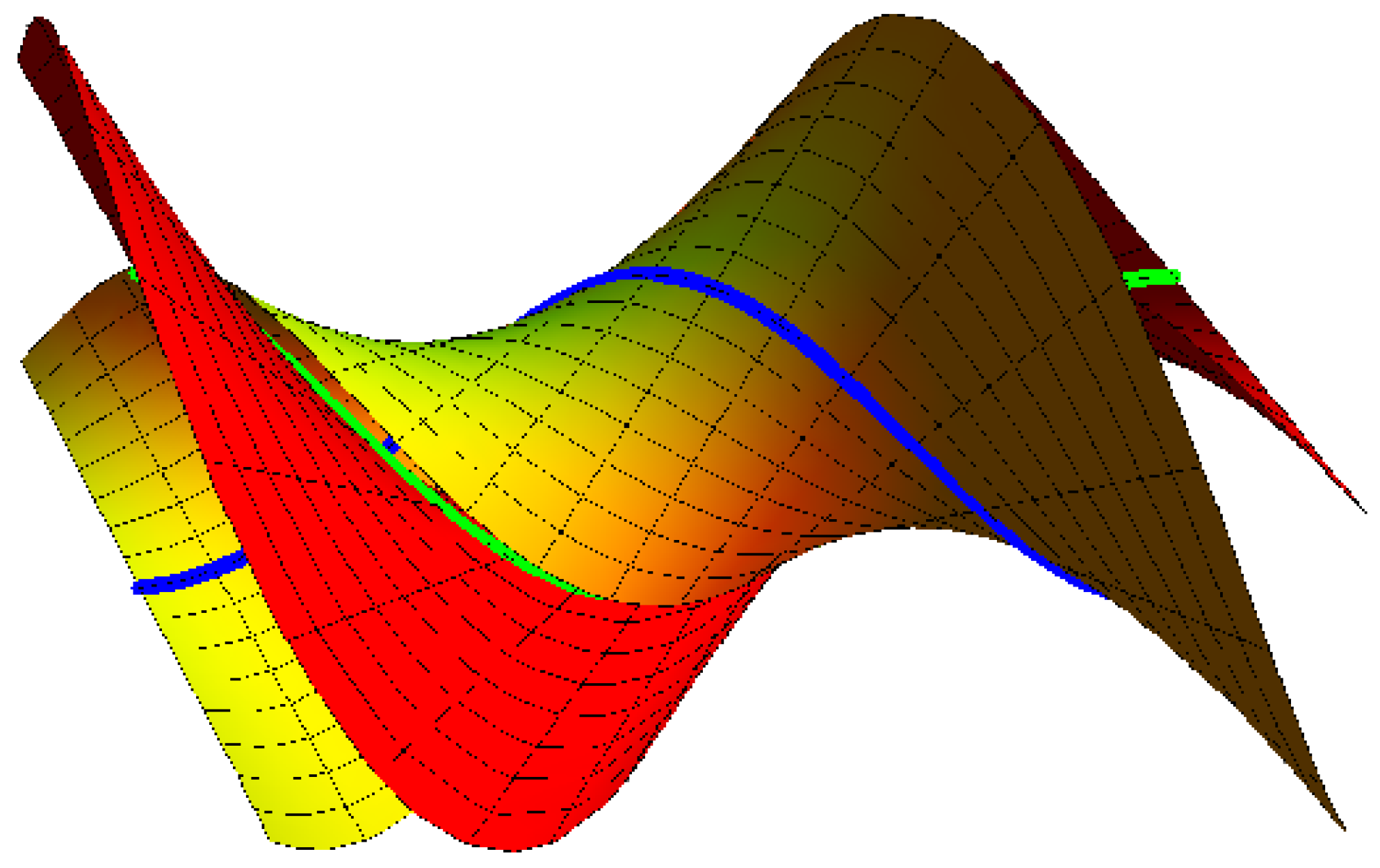
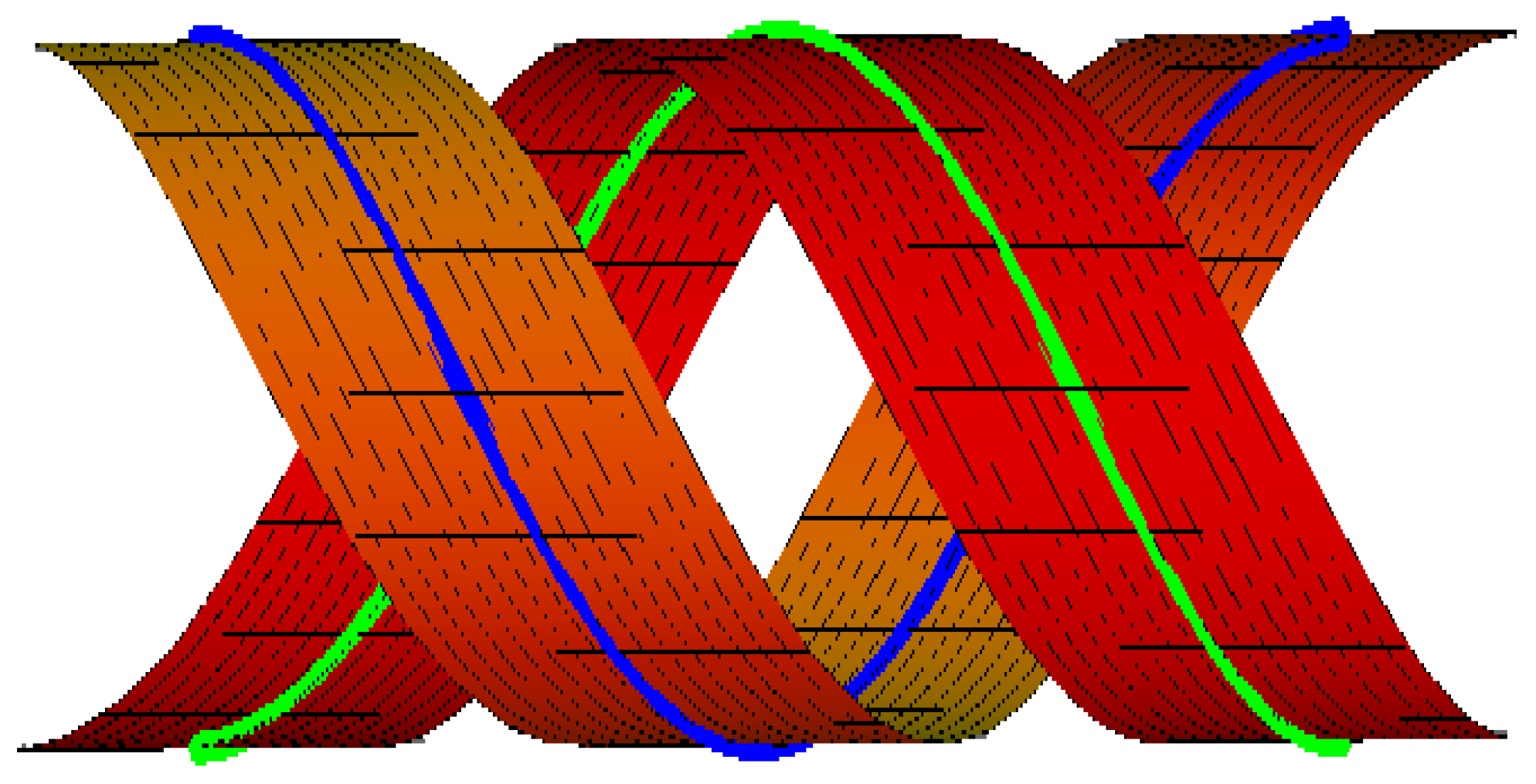
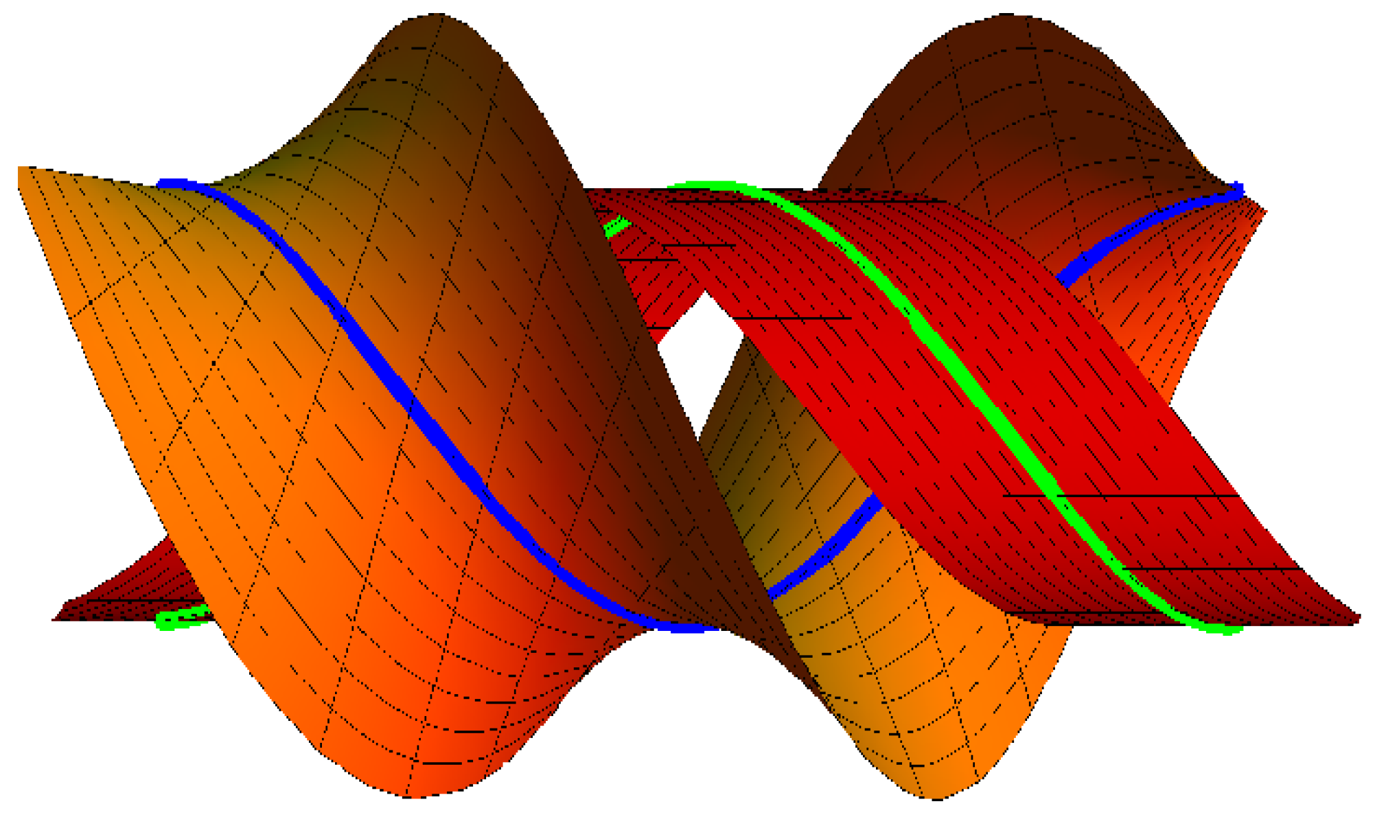
A ruled surface is a special surface created by a continual movable of a line (ruling) on a curve, which acts as the base curve. In this subsection, we address the establishment of the ruled surfaces family with common asymptotic Bertrand curves. To relax the search, let us consider that $\widehat{\mathit{\alpha }}\left(s\right)$ is a unit speed curve. Suppose that $\widehat{\mathit{y}}(s,t)$ is a ruled surface with the base $\widehat{\mathit{\alpha }}\left(s\right)$, and $\widehat{\mathit{\alpha }}\left(s\right)$ is also an isoparametric curve of $\widehat{\mathit{y}}(s,t)$, then there exists $t_0$ such that $\widehat{\mathit{y}}(s,t_0)=\widehat{\mathit{\alpha }}\left(s\right)$. This shows that the surface can be appointed by

$$\widehat{M}:\widehat{\mathit{y}}(s,t)-\widehat{\mathit{y}}(s,t_0)=(t-t_0)\widehat{\mathit{g}}\left(s\right),0\le s\le L,\mathrm{with}t,t_0\in [0,T],$$

where $\widehat{\mathit{g}}\left(s\right)$ is a unit vector specifying the orientation of the rulings. Via the Equation (6), we have

$$(t-t_0)\widehat{\mathit{g}}\left(s\right)=x(s,t){\widehat{\mathit{\upsilon }}}_1\left(s\right)+y(s,t){\widehat{\mathit{\upsilon }}}_2\left(s\right),0\le s\le L,\mathrm{with}t,t_0\in [0,T],$$

(18)

which is a system of two equations with two anonymous functions, $x(s,t)$ and $y(s,t)$. To solve the functions $x(s,t)$ and $x(s,t)$, we have

$$\begin{array}{c}x(s,t)=(t-t_0)<\widehat{\mathit{g}},{\widehat{\mathit{\upsilon }}}_1>=(t-t_0)det(\widehat{\mathit{g}},{\widehat{\mathit{\upsilon }}}_2,{\widehat{\mathit{\upsilon }}}_3),\\ y(s,t)=(t-t_0)<\widehat{\mathit{g}},{\widehat{\mathit{\upsilon }}}_2>=(t-t_0)det(\widehat{\mathit{g}},{\widehat{\mathit{\upsilon }}}_3,{\widehat{\mathit{\upsilon }}}_1).\end{array}$$

(19)

Equation (19) is exactly the necessary and sufficient conditions for $\widehat{\mathit{y}}(s,t)$ to be a ruled surface. In view of Theorem 1, if the curve $\widehat{\mathit{\alpha }}\left(s\right)$ is too much of an asymptotic curve on the surface $\widehat{\mathit{y}}(s,t)$, then $det(\widehat{\mathit{g}},{\widehat{\mathit{\upsilon }}}_3,{\widehat{\mathit{\upsilon }}}_1)\ne 0$. Thus, at any point on the curve $\widehat{\mathit{\alpha }}\left(s\right)$, the ruling guidance $\widehat{\mathit{g}}\left(s\right)\in Sp\{{\widehat{\mathit{\upsilon }}}_1,{\widehat{\mathit{\upsilon }}}_{\mathbf{2}}$}. Furthermore, the vectors $\widehat{\mathit{g}}\left(s\right)$ and ${\widehat{\mathit{\upsilon }}}_1\left(s\right)$ must not be parallel. This leads to

$$\widehat{\mathit{g}}\left(s\right)=\gamma \left(s\right){\widehat{\mathit{\upsilon }}}_1\left(s\right)+\beta \left(s\right){\widehat{\mathit{\upsilon }}}_2\left(s\right),\beta \left(s\right)\ne 0,0\le s\le L,$$

(20)

for the real function $\beta \left(s\right)\ne 0$, and $\gamma \left(s\right)$. Applying it to the Equation (19), we obtain

$$\gamma \left(s\right)t=x(s,t),\beta \left(s\right)t=y(s,t),\beta \left(s\right)\ne 0,0\le s\le L.$$

(21)

Then, the ruled surface family with the common asymptotic $\widehat{\mathit{\alpha }}\left(s\right)$ can be specified as

$$\widehat{M}:\widehat{\mathit{y}}(s,t)=\widehat{\mathit{\alpha }}\left(s\right)+t(\gamma \left(s\right){\widehat{\mathit{\upsilon }}}_1\left(s\right)+\beta \left(s\right){\widehat{\mathit{\upsilon }}}_2\left(s\right)),0\le s\le L,0\le t\le T,$$

(22)

where $\gamma \left(s\right),$ and $\beta \left(s\right)\ne 0$. However, the normal vector to $\widehat{M}$ along the curve $\widehat{\mathit{\alpha }}\left(s\right)$ is

$$\widehat{\mathit{\zeta }}(s,t_0)=\beta \left(s\right){\widehat{\mathit{\upsilon }}}_3\left(s\right),$$

(23)

which shows that $\widehat{\mathit{\alpha }}\left(s\right)$ is an isoasymptotic curve on $\widehat{M}$. Then, the upcoming theorem can be stated.

Theorem 2.

The ruled surfaces family {M, $\widehat{M}$} interpolates {$\mathit{\alpha }\left(s\right)$, $\widehat{\mathit{\alpha }}\left(s\right)$} as common asymptotic Bertrand curves if and only if there exists a parameter $t_0\in [0,T]$ and the functions $\mathit{\alpha }\left(s\right)$, $\beta \left(s\right)\ne 0$, so that $\widehat{M}$ and M, respectively, are parameterized by Equation (23) and

$$M:\mathit{y}(s,t)=\mathit{\alpha }\left(s\right)+t(\mathit{\alpha }\left(s\right){\mathit{\upsilon }}_1\left(s\right)+\beta \left(s\right){\mathit{\upsilon }}_2\left(s\right)),0\le s\le L,0\le t\le T.$$

(24)

It must be pointed out in Equations (22) and (24) that there exist two asymptotic curves crossing via all points on the curve $\widehat{\mathit{\alpha }}\left(s\right)$($\mathit{\alpha }\left(s\right))$; one is $\widehat{\mathit{\alpha }}$ itself, and the other is a line in the guidance $\widehat{\mathit{g}}\left(s\right)$, as given in Equation (21). Every constituent of the isoparametric ruled surface family with the common asymptotic $\widehat{\mathit{\alpha }}$ is established by two set functions, $\mathit{\alpha }\left(s\right)$ and $\beta \left(s\right)\ne 0$.

Example 2.

In view of Example 1, we have the following:

(1)

If $\mathit{\alpha }\left(s\right)=0$, $\beta \left(s\right)=1$, the ruled surfaces family {M, $\widehat{M}$} interpolates {$\mathit{\alpha }(s$), $\widehat{\mathit{\alpha }}\left(s\right)$} as common asymptotic Bertrand curves, as in (Figure 4):

$$\left\{\begin{array}{c}M:\mathit{y}(s,t)=(\frac{1}{\sqrt{2}}coss+\frac{t}{\sqrt{2}}sins,\frac{1}{\sqrt{2}}sins-\frac{t}{\sqrt{2}}coss,\frac{s}{\sqrt{2}}+\frac{t}{\sqrt{2}}),\\ \widehat{M}:\widehat{\mathit{y}}(s,t)=(\frac{-1}{\sqrt{2}}coss-\frac{t}{\sqrt{2}}sins,\frac{-1}{\sqrt{2}}sins+\frac{t}{\sqrt{2}}coss,\frac{s}{\sqrt{2}}+\frac{t}{\sqrt{2}}),\end{array}\right.$$

where $-0.5\le$$t\le 0.5$ and $0\le$$s\le 2\pi$. The blue curve clarifies $\widehat{\mathit{\alpha }}\left(s\right)$ on $\widehat{M}$, and the green curve is $\mathit{\alpha }\left(s\right)$ on M.

(2)

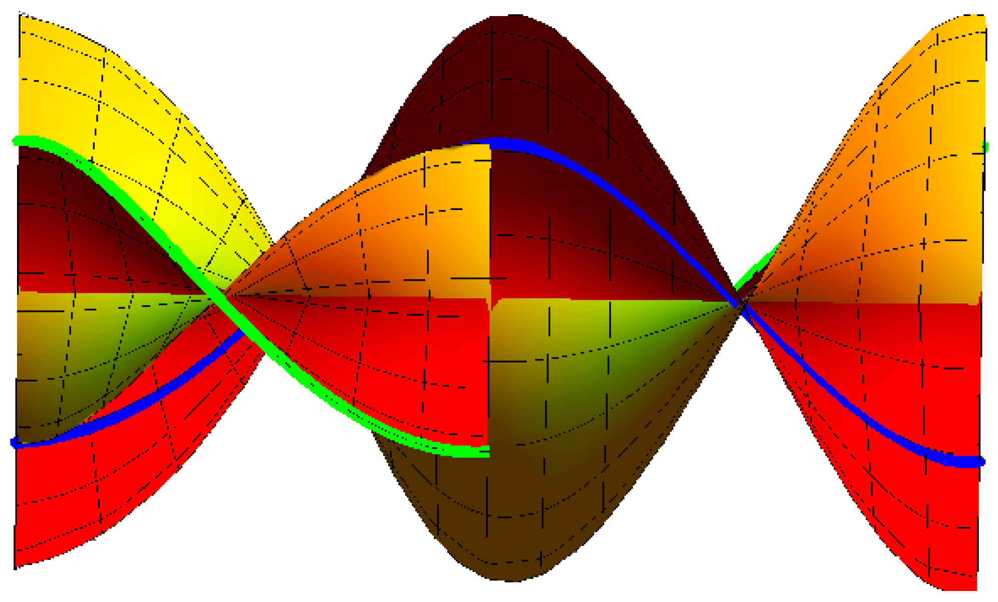
If $\mathit{\alpha }\left(s\right)=\beta \left(s\right)=1$, the ruled surfaces family {M, $\widehat{M}$} interpolates {$\mathit{\alpha }\left(s\right)$, $\widehat{\mathit{\alpha }}\left(s\right)$} as common asymptotic Bertrand curves, as in (Figure 5):

$$\left\{\begin{array}{c}M:\mathit{y}(s,t)=(\frac{1}{\sqrt{2}}coss,\frac{1}{\sqrt{2}}sins,\frac{s}{\sqrt{2}}+\sqrt{2}t),\\ \widehat{M}:\widehat{\mathit{y}}(s,t)=(\frac{-1}{\sqrt{2}}coss,\frac{-1}{\sqrt{2}}sins,\frac{s}{\sqrt{2}}+\sqrt{2}t),\end{array}\right.$$

where $-0.5\le$$t\le 0.5$, and $0\le$$s\le 2\pi$. The blue curve clarifies $\widehat{\mathit{\alpha }}\left(s\right)$ on $\widehat{M}$, and the green curve is $\mathit{\alpha }\left(s\right)$ on M.

(3)

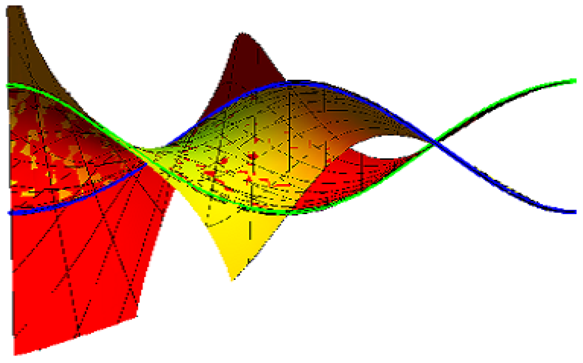
If $\mathit{\alpha }\left(s\right)=-1$, $\beta \left(s\right)=2$, the ruled surfaces family {M, $\widehat{M}$} interpolates {α$\left(s\right)$, $\widehat{\mathit{\alpha }}\left(s\right)$} as common asymptotic Bertrand curves, as in (Figure 6):

$$\left\{\begin{array}{c}M:\mathit{y}(s,t)=(\frac{1}{\sqrt{2}}coss+\frac{3t}{\sqrt{2}}sins,\frac{1}{\sqrt{2}}sins-\frac{3t}{\sqrt{2}}coss,\frac{s}{\sqrt{2}}+\frac{t}{\sqrt{2}}),\\ \widehat{M}:\widehat{\mathit{y}}(s,t)=(-\frac{1}{\sqrt{2}}coss-\frac{3t}{\sqrt{2}}sins,\frac{1}{\sqrt{2}}-sins+\frac{3t}{\sqrt{2}}coss,\frac{s}{\sqrt{2}}+\frac{t}{\sqrt{2}}),\end{array}\right.$$

where $-0.5\le$$t\le 0.5$, and $0\le$$s\le 2\pi$. The blue curve clarifies $\widehat{\mathit{\alpha }}\left(s\right)$ on $\widehat{M},$ and the green curve is $\mathit{\alpha }\left(s\right)$ on M.

4. Conclusions

In this paper, we introduced the notions of surfaces family with common asymptotic curves in Euclidean 3space ${\mathbb{E}}^3$. Subsequently, the outcome for the ruled surfaces family with common asymptotic curves is also deduced. As applications of our main results, some examples are given to construct the surfaces family and ruled surfaces family with common Bertrand asymptotic curves. Hopefully, these results will be advantageous to the work in computer-aided manufacture and those exploring manufacturing. There are many opportunities for further work. The authors plans to register the study in different spaces and examine the classification of the singularities reported in [17,18,19].

References

- Do Carmo, M.P. Differential Geometry of Curves and Surfaces; Prentice-Hall: Englewood Cliffs, NJ, USA, 1976. [Google Scholar]
- Spivak, M.A. Comprehensive Introduction to Differential Geometry, 2nd ed.; Publish or Perish: Houston, TX, USA, 1979. [Google Scholar]
- Contopoulos, G. Asymptotic curves and escapes in Hamiltonian systems. Astron. Astrophys. 1990, 231, 41–55. [Google Scholar]
- Efthymiopoulos, C.; Contopoulos, G.; Voglis, N. Cantori, islands and asymptotic curves in the stickiness region. Celest. Mech. Dynam. Astronom. 1999, 73, 221–230. [Google Scholar] [CrossRef]
- Flory, S.; Pottmann, H. Ruled surfaces for rationalization and design in architecture. In Proceedings of the Conference of the Association for Computer Aided Design in Architecture (ACADIA) (2010), New York, NY, USA, 21–24 October 2010. [Google Scholar]
- Wang, G.J.; Tang, K.; Tai, C.L. Parametric representation of a surface pencil with a common spatial geodesic. Comput. Aided Des. 2004, 36, 447–459. [Google Scholar] [CrossRef]
- Kasap, E.; Akyildiz, F.T.; Orbay, K. A generalization of surfaces family with common spatial geodesic. Appl. Math. Comput. 2008, 201, 781–789. [Google Scholar] [CrossRef]
- Li, C.-Y.; Wang, R.-H.; Zhu, C.-G. Designing approximation minimal parametric surfaces with geodesics. Appl. Math. Model. 2013, 37, 6415–6424. [Google Scholar] [CrossRef]
- Saffak, G.; Kasap, E. Family of surface with a common null geodesic. Int. J. Phys. Sci. 2009, 4, 428–433. [Google Scholar]
- Li, C.Y.; Wang, R.H.; Zhu, C.G. Parametric representation of a surface pencil with a common line of curvature. Comput. Aided Des. 2011, 43, 1110–1117. [Google Scholar] [CrossRef]
- Bayram, E.; Guler, F.; Kasap, E. Parametric representation of a surface pencil with a common asymptotic curve. Comput. Aided Des. 2012, 44, 637–643. [Google Scholar] [CrossRef]
- Li, C.Y.; Wang, R.H.; Zhu, C.G. An approach for designing a developable surface through a given line of curvature. Comput. Aided Des. 2013, 45, 621–627. [Google Scholar] [CrossRef]
- Li, C.Y.; Wang, R.H.; Zhu, C.G. A generalization of surface family with common line of curvature. Appl. Math. Comput. 2013, 219, 9500–9507. [Google Scholar] [CrossRef]
- Papaioannou, S.G.; Kiritsis, D. An application of Bertrand curves and surface to CAD/CAM. Comput. Aided Des. 1985, 17, 348–352. [Google Scholar] [CrossRef]
- Ravani, B.; Ku, T.S. Bertrand offsets of ruled and developable surfaces. Comput. Aided Des. 1991, 23, 145–152. [Google Scholar] [CrossRef]
- Sprott, K.S.; Ravani, B. Cylindrical milling of ruled surfaces. Int. J. Adv. Manuf. Technol. 2008, 38, 649–656. [Google Scholar] [CrossRef]
- Almoneef, A.A.; Abdel-Baky, R.A. Singularity properties of spacelike circular surfaces. Symmetry 2023, 15, 842. [Google Scholar] [CrossRef]
- Li, Y.; Alkhaldi, A.H.; Ali, A.; Abdel-Baky, R.A.; Saad, M. Investigation of ruled surfaces and their singularities according to Blaschke frame in Euclidean 3-space. AIMS Math. 2023, 8, 13875–13888. [Google Scholar] [CrossRef]
- Nazra, S.; Abdel-Baky, R.A. Singularities of non-lightlike developable surfaces in Minkowski 3-space. Mediterr. J. Math. 2023, 20, 45. [Google Scholar] [CrossRef]
Disclaimer/Publisher’s Note: The statements, opinions and data contained in all publications are solely those of the individual author(s) and contributor(s) and not of MDPI and/or the editor(s). MDPI and/or the editor(s) disclaim responsibility for any injury to people or property resulting from any ideas, methods, instructions or products referred to in the content. |
© 2023 by the authors. Licensee MDPI, Basel, Switzerland. This article is an open access article distributed under the terms and conditions of the Creative Commons Attribution (CC BY) license (https://creativecommons.org/licenses/by/4.0/).
Share and Cite
Aldossary, M.T.; Abdel-Baky, R.A. Surfaces Family with Bertrand Curves as Common Asymptotic Curves in Euclidean 3–Space E3. Symmetry 2023, 15, 1440. https://doi.org/10.3390/sym15071440
Aldossary MT, Abdel-Baky RA. Surfaces Family with Bertrand Curves as Common Asymptotic Curves in Euclidean 3–Space E3. Symmetry. 2023; 15(7):1440. https://doi.org/10.3390/sym15071440
Chicago/Turabian StyleAldossary, Maryam T., and Rashad A. Abdel-Baky. 2023. "Surfaces Family with Bertrand Curves as Common Asymptotic Curves in Euclidean 3–Space E3" Symmetry 15, no. 7: 1440. https://doi.org/10.3390/sym15071440