Article

Multi-Strategy Enhanced Dung Beetle Optimizer and Its Application in Three-Dimensional UAV Path Planning

School of Big Data and Information Engineering, Guizhou University, Guiyang 550025, China
*
Author to whom correspondence should be addressed.
Symmetry 2023, 15(7), 1432; https://doi.org/10.3390/sym15071432
Submission received: 2 June 2023 / Revised: 4 July 2023 / Accepted: 13 July 2023 / Published: 17 July 2023
(This article belongs to the Topic Applied Metaheuristic Computing: 2nd Volume)

Abstract

:
Path planning is a challenging, computationally complex optimization task in high-dimensional scenarios. The metaheuristic algorithm provides an excellent solution to this problem. The dung beetle optimizer (DBO) is a recently developed metaheuristic algorithm inspired by the biological behavior of dung beetles. However, it still has the drawbacks of poor global search ability and being prone to falling into local optima. This paper presents a multi-strategy enhanced dung beetle optimizer (MDBO) for the three-dimensional path planning of an unmanned aerial vehicle (UAV). First, we used the Beta distribution to dynamically generate reflection solutions to explore more search space and allow particles to jump out of the local optima. Second, the Levy distribution was introduced to handle out-of-bounds particles. Third, two different cross operators were used to improve the updating stage of thief beetles. This strategy accelerates convergence and balances exploration and development capabilities. Furthermore, the MDBO was proven to be effective by comparing seven state-of-the-art algorithms on 12 benchmark functions, the Wilcoxon rank sum test, and the CEC 2021 test suite. In addition, the time complexity of the algorithm was also analyzed. Finally, the performance of the MDBO in path planning was verified in the three-dimensional path planning of UAVs in oil and gas plants. In the most challenging task scenario, the MDBO successfully searched for feasible paths with the mean and standard deviation of the objective function as low as 97.3 and 32.8, which were reduced by 39.7 and 14, respectively, compared to the original DBO. The results demonstrate that the proposed MDBO had improved optimization accuracy and stability and could better find a safe and optimal path in most scenarios than the other metaheuristics.

1. Introduction

Artificial intelligence is one of the most promising technologies for solving problems in various fields. UAV is a powerful auxiliary tool in artificial intelligence technology with high flexibility, low cost, and high efficiency [1]. It is also considered as a candidate technology for future 6G networks and has wide applications in various scenarios [2]. For example, in hazardous areas such as oil and gas plants, UAVs can replace humans to perform specific tasks and improve work efficiency. However, ensuring the safety of autonomous flight UAVs in complex environments is a significant challenge. Path search has essential research significance as a supporting technology for UAV flight. Path planning allows the UAV to find the optimal safe path from a start point to an endpoint according to specific optimization criteria such as the minimal path length or the lowest energy consumption [3]. The UAV path searching problem is based on the case of task points and prior maps. Therefore, the mission, the surrounding environment, and the UAV’s physical constraints should be clarified first. On this basis, the task requirements, environmental states, and constraints related to UAVs are expressed through a mathematical model and applied to the path-planning problem. It has been proven that finding the optimal path is an NP-hard problem [4], and the complexity of the problem increases rapidly with the size of the problem.
Many researchers have been trying to develop solutions to path-planning problems, for example, conventional methods such as the artificial potential algorithm [5] and the Voronoi diagram search method [6]; cell-based methods such as Dijkstra [7] and the A-Star algorithm [8]; model-based methods such as rapidly exploring random tree (RRT) [9]; learning-based methods such as neural networks [10] and the evolutionary computation technique [11]. However, the limitations of the traditional and cell-based methods lie in poor flexibility and fault tolerance. The model-based methods typically have complex modeling and cannot work in real-time path planning. Neural networks have low complexity, flexibility, and fault tolerance advantages. Nevertheless, most neural networks require a learning process, which is time-consuming. Due to the limitations of traditional methods to successfully solve optimal paths, researchers have proposed metaheuristic algorithms for solving path-planning problems inspired by natural phenomena or laws, for example, genetic algorithm (GA) [12], particle swarm optimization (PSO) [13], ant colony optimization (ACO) [14], differential evolution (DE) [15], fruit fly optimization algorithm (FOA) [16], and the grey wolf optimization (GWO) algorithm [17]. The dung beetle optimization algorithm [18] is a recently developed metaheuristic algorithm that imitates the biological behavior of dung beetles. However, a determined metaheuristic cannot perform well in all categories of optimization problems, a hypothesis already proven by the “No Free Lunch” theorem [19]. This paper aimed to develop an efficient optimization algorithm for solving three-dimensional path-planning problems in oil and gas plants.
Nowadays, researchers have proposed many improved metaheuristic algorithms for solving various engineering application problems including path-planning problems. Yu X. et al. [15] modeled UAV path planning as a constraint satisfaction problem, in which the fitness function included the travel distance and risk of the UAV. Three constraints considered in the problem were UAV height, angle, and limited UAV slope. Jain et al. [20] proposed the multiverse optimizer (MVO) algorithm to deal with the coordination of UAVs in a three-dimensional environment. The results showed that the MVO algorithm performed better in most testing scenarios with the minimum average execution time. Li K. et al. [21] focused on multi-UAV collaborative task assignment problems with changing tasks. They proposed an improved fruit fly optimization algorithm (ORPFOA) to solve the real-time path-planning problem. Pehlivanoglu et al. [12] considered the path-planning problem of autonomous UAVs in target coverage problems and proposed initial population enhancement methods in GA for efficient path planning. These techniques aim to reduce the chances of collisions between UAVs.
Zhang X. et al. [22] proposed an improved FOA (MCFOA) by introducing two new strategies, Gaussian mutation and chaotic local search. Then, the MCFOA was applied to the feature selection problem to verify its optimization performance. Song S. et al. [23] used two different Gaussian variant strategies and dimension decision strategies to design an enhanced HHO (GCHHO) algorithm. The GCHHO algorithm has successfully optimized engineering design problems (such as tensile/compression springs and welded beam design problems). Gupta S. et al. [24] presented an improved random walk grey wolf algorithm and applied it to the parameter estimation of the frequency modulation (FM) unconstrained optimization problem, the optimal capacity of production facilities, and the design of pressure vessels. Pichai [25] introduced asymmetric chaotic sequences into the competitive swarm optimization (CSO) algorithm and applied it to the feature selection of high-dimensional data. The results showed that the algorithm reduced the number of features and improved the accuracy. Mikhalev [26] proposed a cyclic spider algorithm to optimize the weights of recurrent neural networks, and the results showed that the algorithm reduced the prediction errors. Almotairi [27] proposed a hybrid algorithm based on the reptile search algorithm and the remora algorithm, improving the original algorithm’s search capability. Then, the hybrid algorithm was applied to the cluster analysis problem.
Previous work has deeply studied the defects of intelligent algorithms and improved the convergence ability of algorithms. In this paper, we improved the optimization ability of the DBO and the solving efficiency of the UAV path-planning problem. The following work was conducted to improve the search performance of the DBO:
  • Adding a reflective learning strategy and using Beta distribution function mapping to generate reflective solutions, improving the algorithm’s search ability;
  • For particles that exceeded the search space range, Levy distribution mapping was used to handle particle boundaries, enhancing the probability of global search reaching the optimal position;
  • Individual crossover mechanism and dimension crossover mechanism were used to update the position of individual thief beetles, increasing the population diversity and avoiding falling into local optima;
  • Applying the improved MDBO to solve the three-dimensional UAV path-planning problem, and design sets of scene experiments to verify the efficiency of the MDBO.
The rest of this paper is organized as follows. Section 2 illustrates the basic DBO. In Section 3, the proposed MDBO is described in detail. In Section 4, the experimental results of the proposed MDBO are analyzed. Section 5 describes the UAV path-planning model. Section 6 conducts the UAV planning simulation experiments and discusses the comparison results between the MDBO and other metaheuristic algorithms. Finally, Section 7 provides a summary of the paper.

2. Dung Beetle Optimizer (DBO)

The basic DBO is based on population, mainly inspired by the ball-rolling, dancing, foraging, stealing, and reproduction behaviors of dung beetles. The DBO divides the population into four search agents: ball-rolling dung beetle, brood ball, small dung beetle, and thief. Specifically, each search agent has its own unique updating rules. Note that specific details will be described as follows.
(1)
Ball-rolling dung beetle
During the rolling process, dung beetles must navigate through celestial cues to keep the dung ball rolling in a straight line. Thus, the position of the ball-rolling dung beetle is updated and can be expressed as:
x i ( t + 1 ) = x i ( t ) + α × k × x i ( t 1 ) + b × Δ x
Δ x = | x i ( t ) X w |
where t represents the current number of iterations; x i ( t ) represents the position information of the ith dung beetle during the tth iteration; k ( 0 , 0.2 ] is a constant value representing the deflection coefficient; b is a constant value belonging to (0,1); α is a natural coefficient assigned to 1 or −1; X w is the global worst position; Δ x simulates changes in light intensity.
When a dung beetle encounters obstacles that prevent it from progressing, it will redirect itself through dancing to obtain a new route. A tangent function simulates the dancing behavior to obtain a new rolling direction. Therefore, the location of the ball-rolling dung beetle is updated as follows:
x i ( t + 1 ) = x i ( t ) + tan ( θ ) | x i ( t ) x i ( t 1 ) |
where θ [ 0 , π ] is the deflection angle.
(2)
Brood ball
Choosing a suitable spawning site is crucial for dung beetles to provide a safe environment for their offspring. Hence, in DBO, a boundary selection strategy is proposed to simulate the spawning area of female dung beetles, which is defined as follows:
L b * = max ( X * × ( 1 R ) ,   L b ) U b * = min ( X * × ( 1 R ) ,   U b )
where X * represents the current local optimal position; L b * and U b * represent the lower and upper bounds of the spawning area; R = 1 t / T max ; T max denotes the maximum number of iterations; L b and U b are the lower and upper bounds of the search space, respectively.
It is assumed that each female dung beetle will only lay one egg in each iteration. The boundary range of the spawning area changes dynamically with values, so the position of the egg ball also changes dynamically during the iteration process expressed as follows:
B i ( t + 1 ) = X * + b 1 × ( B i ( t ) L b * ) + b 2 × ( B i ( t ) U b * )
where B i ( t ) is the position of the ith sphere at the tth iteration; b 1 and b 2 are two independent random vectors with a size of 1 × D ; D is the dimension.
(3)
Small dung beetle
Some adult dung beetles will burrow out of the ground in search of food, and this type of dung beetle is called the small dung beetle. The boundaries of the optimal foraging area for small dung beetles are defined as follows:
L b b = max ( X b × ( 1 R ) ,   L b ) U b b = min ( X b × ( 1 R ) ,   U b )
where X b represents the global optimal position; L b b and U b b are the lower and upper bounds of the optimal foraging area, respectively. Therefore, the location of the small dung beetle is updated as follows:
x i ( t + 1 ) = x i ( t ) + C 1 × ( x i ( t ) L b b ) + C 2 × ( x i ( t ) U b b )
where x i ( t ) represents the position of the ith dung beetle at the tth iteration; C 1 is the random number subject to normal distribution; C 2 is the random vector within the range of (0,1).
(4)
Thief
Some dung beetles, known as thieves, steal dung balls from other beetles. From Equation (5), it can be observed that X b is the optimal food source. Assume that the area around X b is the optimal location for competing food. During the iteration process, the location information of the thief is updated as follows:
x i ( t + 1 ) = X b + S × g × ( | x i ( t ) X * | + | x i ( t ) X b | )
where x i ( t ) represents the location information of the ith thief at the tth iteration; g is a random vector subject to normal distribution with the size of 1 × D ; S is a constant value.

3. The Proposed Method

The MDBO proposed in this section mainly includes three strategies: generating reflective solutions, handling position boundary violations, and improving thief dung beetle position updates.

3.1. Dynamic Reflective Learning Strategy Based on Beta Distribution

The dynamic region selection strategy proposed by DBO strictly limits the search scope to this region, which is not conducive to searching other regions. The search scope can be expanded by dynamically calculating the solution in the opposite direction, helping the original algorithm break away from the local optimal region. The traditional method of randomly generating initial positions according to uniform distribution is simple and feasible. It is adverse to forming an “encircling” to the optimal solution. This paper proposes generating reflective solutions using Beta distribution to effectively surround the optimal solution with the initial position.
The Beta distribution function is defined as:
f ( x ) = 1 B ( α , β ) x α 1 ( 1 x ) β 1 ,   x [ 0 , 1 ]
where B ( α , β ) is the Beta function, defined as:
B ( α , β ) = 0 1 t α 1 ( 1 t ) β 1 d t
Figure 1 shows the probability density function of the Beta distribution. From the figure, it can be seen that when α = β = 0.5 , the shape of the density function is symmetric in a U-shape. The candidate solution generated is most likely located near the boundary of the search space, so the global optimal solution is better “surrounded” within the initial particle swarm.
Assume that the number of particles is N, the dimension is D, the maximum number of iterations is T, the upper and lower bounds of the jth dimension are [ L b j , U b j ], and the reverse solution is u , generated according to the following formulas:
u i , j ( t + 1 ) = { r i , j ( t + 1 ) i f ( x i , j ( t + 1 ) s j ) p i , j ( t + 1 ) i f ( x i , j ( t + 1 ) < s j ) , i [ 1 , N ] ,   j [ 1 , D ] ,   t [ 1 , T ]
r i , j ( t + 1 ) = { Φ ( U b j + L b j x i , j ( t + 1 ) ,   s j )   i f ( | x i , j ( t + 1 ) s j | | U b j L b j | < Φ ( 0 , 1 ) ) Φ ( L b j ,   U b j + L b j x i , j ( t + 1 ) ) o t h e r w i s e
p i , j ( t + 1 ) = { Φ ( s j ,   U b j + L b j x i , j ( t + 1 ) )   i f ( | x i , j ( t + 1 ) s j | | U b j L b j | < Φ ( 0 , 1 ) ) Φ ( U b j + L b j x i , j ( t + 1 ) ,   U b j ) o t h e r w i s e
s j = 1 2 ( U b j + L b j )
Φ ( a , b ) = a + ( b a ) × betarnd ( α , β )
where x i , j ( t + 1 ) is the jth value of the ith solution at the t + 1th iteration; u i , j ( t + 1 ) is the jth value of the ith reflective solution at the t + 1th iteration; s j is the domain center of the upper and lower boundaries; Φ ( a , b ) generated a random number within ( a , b ) that follows the Beta distribution; betarnd is a function to randomly generate a number that obeys the Beta distribution. In this article, α = β = 0.5.

3.2. Cross Boundary Limits Method Based on Levy Distribution

The simple method of “if the particle exceeds the boundary, it is equal to the boundary” is used to deal with the individual position. The advantage of this method is that it is simple to implement. However, because the boundary point is not the global optimal solution, this method is unfavorable to the optimization process. In this paper, a new boundary processing method based on Levy distribution mapping was adopted. The specific operations are as follows:
x i j = { min ( U b j L e v y ( λ ) , U b j ) , x i j > U b j max ( L b j , L b j L e v y ( λ ) ) , x i j < L b j
where x i j is the particle position after boundary processing; λ is a constant number; Levy is a random search path, and its random step size is a Levy distribution. The notation is entry-wise multiplications. Figure 2 visually shows the method for handling particle boundaries. When the particle x i j jumps out of the upper and lower boundaries, it re-enters the search region using Levy steps with random jumps.

3.3. Cross Operators for Updating the Location of Thieves

As can be seen from Equation (8), the thief’s position is affected by the global optimal solution. This mechanism enables the optimal solution to be generated by the thieves. However, once the optimal individual falls into the local optimal solution, the solving efficiency of the algorithm will be greatly reduced. Inspired by the crisscross optimizer [28], this paper introduced horizontal and vertical crossover operators to perform crosstalk operations on thieves to improve the convergence ability of the algorithm. Note that specific details are described as follows.
(1)
Horizontal crossover search (HCS)
HCS is similar to the crossover operation in genetic algorithms, which involves performing crossover operated on all dimensions between two individuals. Assuming that the dth dimension of the parent individual x i and x j are used to perform HCS, their kids can be reproduced as:
M S i , d = ε 1 × x i , d + ( 1 ε 1 ) × x j , d + c 1 × ( x i , d x j , d )
M S j , d = ε 2 × x j , d + ( 1 ε 2 ) × x i , d + c 2 × ( x j , d x i , d )
where ε 1 and ε 2 are random numbers uniformly distributed in the range of (0,1); c 1 and c 2 are random numbers uniformly distributed in the range of (−1,1). M S i , d and M S j , d are the kids generated by x i , d and x j , d , respectively.
(2)
Vertical crossover search (VCS)
VCS is a crossover operation performed between two dimensions of the corresponding individuals, which has a lower probability of occurrence than HCS. Assume that the d1th and d2th dimensions of the individual i are used to perform VCS, which is calculated as follows:
M S i , d 1 = ε × x i , d 1 + ( 1 ε ) × x i , d 2
where ε is random number uniformly distributed in the range of (0,1), and M S i , d 1 is the offspring of x i , d 1 and x i , d 2 .

3.4. The Detailed Process of the MDBO

By introducing the above three strategies into the MDBO, the convergence speed and convergence accuracy of the algorithm can be effectively improved to balance the global exploration and local exploitation while enhancing the performance of the original DBO.
Figure 3 shows the process of MDBO implementation.
The pseudo-code of MDBO is shown in Algorithm 1.
Algorithm 1: The pseudo code of MDBO
Initialize the particle’s population N; the maximum iterations T; the dimensions D.
Initialize the positions of the dung beetles
While tT do
 Calculate the current best position and its fitness
 Obtain N reflective solutions by Equations (11)–(15)
 Update the positions of N individuals
For i = 1:N do
   if i == ball-rolling dung beetle then
   Generate a random number p ( 0 , 1 )
   if p < 0.9 then
   Update search position by Equation (1)
   Else
   Update search position by Equation (3)
   end if
   if i == brood ball then
   Update search position by Equation (5)
   end if
   if i == small dung beetle then
   Update search position by Equation (7)
   end if
   if i == thief then
   Update search position by Equation (8)
   while tT/4 do
    Perform HCS using Equations (17)–(18)
    Perform VCS using Equation (19)
   end while
   end if
end for
 Update the best position and its fitness
 t = t + 1
end while
Return the optimal solution Xb and its fitness fb.

3.5. Computational Complexity Analysis

The pseudo-code of the proposed algorithm is shown in Algorithm 1. The complexity of the optimizer is one of the key indicators that can reflect the algorithm’s efficiency. According to the pseudo-code in Algorithm 1, it can be seen that the complexity of MDBO mainly includes these several processes: initialization; calculating the reflective solutions by Beta distribution; HCS and VCS; updating the dung beetles’ position with new boundary handling method. For convenience, it was assumed that N solutions and T iterations are involved in the optimization process of a D-variable problem. First, the complexity in the initialization phase is O ( N ) . Then, the complexity level of calculating N reflective solutions is O ( T N ) . The complexity level of HCS and VCS is O ( T N D + T N N ) . In MDBO, the total number of evaluations in updating the particles’ position is 4 T N because N group solutions are evaluated per cycle. Thus, the time complexity of the dung beetles to look for the best position is about O ( 4 T N ) , which can be abbreviated as O ( T N ) . Based on the above discussions, the overall time complexity of MDBO is O ( M D B O ) = O ( N + T N ( 1 + D + N ) ) . Compared to DBO, although it increases the time overhead, the performance is optimized.

4. Analysis of Simulation Experiments

4.1. Experimental Design

In this section, a series of numerical experiments on MDBO were conducted to validate the effectiveness of MDBO. The statistical analysis and convergence analysis were performed on 12 basic benchmark functions [29,30,31] and CEC2021 competition functions [32]. Four well-established optimization techniques (the POA [33], SCSO [34], HBA [35], and DBO [18]), and three improved metaheuristics in recent years (the ISSA [36], MCFOA [22], GCHHO [23]) were compared with our proposed MDBO. Table 1 shows the parameter settings of all algorithms. For fairness, the population size N = 30 for all algorithms, and the maximum iterations T = 500. Mean (Mean) and standard deviation (Std) are used as statistical indicators to assess the optimization performance. All experiments were achieved on MatlabR2019a version.

4.2. Sensitivity Analysis of MDBO’s Parameters

This section analyzes the sensitivity of the control parameters (k, b, α, β) employed in the MDBO. The parameters k and b are consistent with the values taken in the DBO. Xue [18] has demonstrated that the algorithm performance is the most robust when k = 0.1, b = 0.3. In this subsection, we focused on analyzing the effect of the added parameters α and β on the search performance of the algorithm. Four CEC test functions (including the unimodal function CEC-1, the basic function CEC-3, the hybrid function CEC-7, and the composition function CEC-10) were used to test the design of these control parameters. Five parameter combinations, { α = 0.5 ,   β = 0.5 } , { α = 5 ,   β = 1 } , { α = 1 ,   β = 3 } , { α = 2 ,   β = 2 } , and { α = 2 ,   β = 5 } , were set according to different distributions.
The sensitivity analysis is shown in Figure 4, where the horizontal coordinates indicate the five parameter combinations, and the vertical coordinates indicate the mean values. It can be seen from Figure 4a,c that the algorithm performed optimally when α = 0.5 and β = 0.5. For CEC1, α and β showed a high sensitivity to different inputs. Noting that a = 0.5 and b = 0.5 had the best performance. Moreover, we could see that α = 0.5 and β = 0.5 could obtain the best search performance in CEC7. It is observable in Figure 4b,d that α = 0.5 and β = 0.5 demonstrated the robust behavior of different inputs. For CEC3, from the values displayed in the vertical coordinates, the optimized objective function values obtained for various combinations of a and b were relatively close. Note that α = 0.5 and β = 0.5 obtained second place after α = 2 and β = 2. In CEC10, the performance of α = 2 and β = 5 was better than that of α = 2 and β = 2. However, α = 0.5 and β = 0.5 still achieved second place, showing their robust performance. Therefore, α = 0.5 and β = 0.5 were selected as the recommended parameter values for MDBO.

4.3. Comparison of Performance on 12 Benchmark Functions

The 12 basic benchmark functions included seven unimodal functions and six multimodal functions (details in Appendix A, Table A1). It is worth noting that F1–F7 are typical unimodal test functions since they have one and only one global optimal value. The multimodal functions F8–F12 have features with multiple local optimums. Therefore, F1–F7 are widely used to estimate the convergence accuracy and speed, and F8–F12 are more suitable for testing the global exploration ability. Moreover, to fairly compare the comprehensive search ability of each metaheuristic, all algorithms were independently run 30 times in each experiment. We also tested the scalability and compared the performance of MDBO on dimensions of 30, 50, and 100. Two indicators were used to measure their optimization performance: the mean value (Mean) and the standard deviation (Std).
Table 2 shows the mean and standard deviation data of all algorithms on the 12 benchmark test functions tested, and the table also provides the comparison results of the algorithms when the test functions were taken in 30, 50, and 100 dimensions, respectively. As can be seen from Table 2, MDBO achieved the best results in all of the test functions. From the perspective of vertical comparison, MDBO ranked first in the test of other functions, except for some algorithms that showed a comparable performance to MDBO in the F9, F10, and F11 functions. For functions F1–F6, MDBO converged to the theoretical optimal value of 0. For F7 and F8, although MDBO could not have the best value, it showed significant advantages compared with other algorithms. Next, from the results of the dimension comparison, the results of 100 dimensions, 30 dimensions, and 50 dimensions were similar, with little change in the order of optimal value. Based on the above analysis, it can be seen that MDBO has more significant competitive advantages in solving unimodal and multimodal functions. The results reflect the ability to jump out of the local optima by the reflective learning operator and crisscross optimizer.

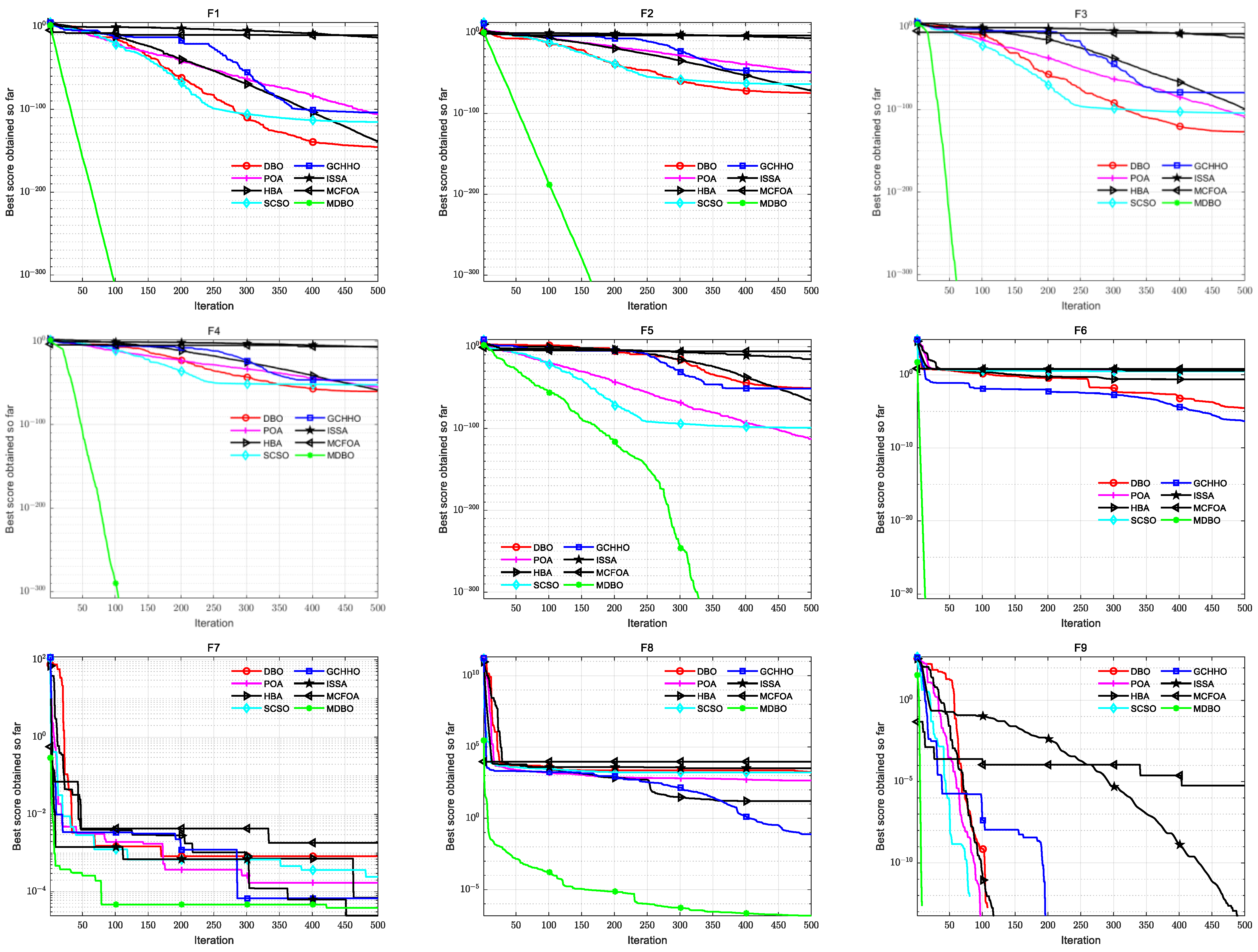
4.4. Convergence Curve Analysis

Convergence analysis plays a vital role in evaluating the ability of the local exploitation and global exploration of the algorithm. Figure 5 shows the convergence curves of DBO, POA, HBA, SCSO, ISSA, GCHHO, MCFOA, and MDBO on functions F1–F12. As shown in Figure 5, MDBO’s optimization ability was the best in 11 (F1–F6, F8–F12) out of 12 functions. For functions F1–F6, the MDBO’s curves dropped rapidly in early iterations and kept a fast convergence rate to the optimal solution. Notably, F1–F5 are continuous unimodal test functions, and MDBO can quickly search for the optimal theoretical value of 0. Since the vertical coordinates of the convergence curve were generated by the logarithmic scale, the accuracy of the displayed magnitude was 10−300. For F4, the function curve of MDBO showed an inflection point because crossover operators can help MDBO re-exploit the optimization precision. For function F7, although the progress of convergence to 500 generations was not as good as that of ISSA, the average number of iterations of function curve convergence to the optimal value was the least and converged to the optimal value in about 100 generations. In F9 and F11, MDBO obtained the optimal global value of 0. The curve broke during iterations because the figure showed an average best value in logarithmic. For functions F8, F10, and F12, MDBO exhibited a more competitive performance than the other comparison algorithms. In summary, convergence analysis proved that MDBO had a higher success ratio than the other optimization algorithms.

4.5. Wilcoxon Rank-Sum Test

To further test the effectiveness of the MDBO, the Wilcoxon rank sum test [37] was used to determine whether there was a statistical difference. Each algorithm was run 30 times independently, and the data volume met the requirement of statistical analysis. Table 3 shows the p-values of the Wilcoxon rank sum test at the α = 5% significance level. If p < 0.05, the original hypothesis is rejected, and the alternative hypothesis is accepted. In Table 3, “+/−/=” indicates the number of MDBO with better/worse/comparable performance compared with other algorithms, respectively, where the ‘’NaN’’ markers had comparable performance. In general, most of the p-values of the rank sum test were less than 0.05. This indicates that the performance of MDBO was significantly different from other algorithms. Therefore, it was considered that the proposed MDBO had excellent convergence performance.

4.6. MDBO’s Performance on CEC2021 Suite

To further verify the performance of the MDBO, the challenging CEC 2021 test suite (details in Appendix A, Table A2) was used to test against the seven metaheuristics above-mentioned. Similarly, for CEC2021, the population size was set to 30, along with 500 maximum iterations, and the dimension was set to 20. Each metaheuristic was run independently 30 times to keep fairness and objectivity. The Wilcoxon signed-rank test (signed-rank test) [37] was also carried out. The symbol “gm” is the score representing the difference between the number of symbols “+” and “−”.
Table 4 shows the experimental results of the MDBO and other optimizers. In Table 4, the proposed MDBO ranked first in CEC-1, CEC-3, CEC-4, and CEC-6. For CEC-2 and CEC-9, MDBO achieved the best mean results compared with other algorithms. For CEC-10, the mean value of MDBO was second only to HBA, but the standard deviation was smaller and more stable than HBA. The “gm” score showed that the MDBO differed significantly from other algorithms in the vast majority of cases. Overall, the results of the CEC2021 test functions show that the MDBO is effective and suitable for some engineering problems.

5. UAV Path-Planning Model

5.1. Environment Model

In the route planning of an UAV inspection in oil and gas plants, it is vital to create an appropriate environment model as it will improve the efficiency of the optimization algorithm. Considering some objects as obstacles in oil and gas plants such as complex pipelines, oil wells, signal towers, and so on, this paper adopted the geometric description method to establish the three-dimensional environment model. In this model, the obstacles are described by cuboids of different sizes. The transformation process of the model is shown in Figure 6. In addition, compared with the military UAV, the inspection UAV does not need to consider threats such as missiles, radar, and anti-aircraft guns. After ensuring the limitations of the UAV, the final optimal path is generated according to the surrounding environment and the task requirements to complete the inspection task. In order to prevent the UAV from colliding with obstacles during the flight, the safety threshold R s a f e is added to the length, width, and height of different cuboids.

5.2. Path Representation

In this paper, it was assumed that the planning path had a start point S and an end point E . During the inspection, the UAV needs to traverse some task points with no collisions. Assume that the path can be represented as a series of discrete points such as ( p 0 ,   p 1 ,   p 2 ,   ,   p k , ,   p n + 1   ) , where the first and last waypoints are the given start and target point. The coordinates of p k are ( x k ,   y k ,   z k ) . The generation of the initial path is introduced as follows:
Step 1, confirm the direction of the next point to the starting point S . The direction of the UAV in three-dimensional space can be generated as:
D I R = ( d i r x , d i r y , d i r z ) ,   d i r x ,   d i r y ,   d i r z [ 1 , 0 , 1 ]
where D I R represents the removable direction, and d i r x ,   d i r y ,   d i r z are the direction on the x-axis, y-axis, and z-axis, respectively.
Then, the next movable waypoint is expressed as:
{ x i + 1 = x i + d i r x r a n d ( ) y i + 1 = y i + d i r y r a n d ( ) z i + 1 = z i + d i r z r a n d ( )
where ( x i ,   y i ,   z i ) is the position of the ith discrete point.
Step 2, make sure that the generated waypoints stay within the map and do not collide with the obstacles. Therefore, it is necessary to penalize infeasible solutions. The penalty function h 1 is introduced as:
h 1 = p I n O b s t a c l e s + p O u t M a p = 0
where p I n O b s t a c l e s is the point of collision with the obstacles, and p O u t M a p denotes the point outside the map.
Step 3, find the optimal waypoint that satisfies the conditions and add it to the path, which can be described as follows:
min   h 2 = ( D 1 + D 2 ) p r i
D 1 = ( x i + 1 x i ) 2 + ( y i + 1 y i ) 2 + ( z i + 1 z i ) 2
D 2 = ( x i x n + 1 ) 2 + ( y i y n + 1 ) 2 + ( z i z n + 1 ) 2
where i is the index of discrete points from 0 to n; p r i is a constant value that depends on the scale of the search space; D 1 and D 2 represent the Euclidean distance between the current path point and the next path point and the end point, respectively.
Step 4, repeat the above operation until the UAV flies to the first task point.
Step 5, finally, repeat the above steps until the UAV flies over all task points and generates a complete initial path.

5.3. Cost Function and Performance Constraints

The objective function that evaluates a candidate route should take account of the cost of the path and the performance, which is expressed as follows:
min   f ( x ) = m = 1 3 w m f m ( x )
L i x i U i ,   i = 1 ,   2 ,   ,   D
where f ( x ) represents the overall cost function; w m is the weight coefficient; f 1 ( x ) to f 3 ( x ) are respectively the costs associated with the path length, flight height, and smoothness. The decision variable is x = { x 1 ,   x 2 ,   , x D } , and D is the dimension of the problem space. L i and U i are the lower and upper bounds of the search space. The cost function and constraints of the UAV path are described as follows:
(1)
Length cost
In the inspection of UAVs, the shorter the path, the less the time and energy consumption. The cost function f 1 is the length of the UAV path, which can be calculated by the Euclidean operator as follows:
f 1 = k = 0 N d k
d k = ( x k + 1 x k ) 2 + ( y k + 1 y k ) 2 + ( z k + 1 z k ) 2
where k is the index of discrete points from 0 to N .
(2)
Flight altitude cost
During the flight, maintaining a steady altitude can reduce the power consumption. In order to ensure the safety of the flight, the altitude of the UAV is usually limited between two given extrema, the minimum height h min and the maximum height h max , respectively. Therefore, the cost function f 2 is computed as:
f 2 = k = 0 N h k
h k = { | z k ( h max + h min ) 2 | , i f   h min z k h max , o t h e r w i s e
where z k denotes the flight height with respect to the ground, and k is the index of waypoints. It should be mentioned that h k maintains the average height and penalizes the values outside the range.
(3)
Smooth cost
To ensure that the UAV can always maintain a good attitude during the working flight, this paper adopted a smooth cost, consisting of the climb turning angle and climbing rates. As shown in Figure 7, the turning angle ϕ k is the angle between two adjacent consecutive path segments. If e 3 is the unit vector in the z-axis direction, the projected vector is calculated as:
p k p k + 1 = e 3 × ( p k p k + 1 × e 3 )
The turning angle is calculated as:
ϕ k = arctan   ( p k p k + 1 × p k + 1 p k + 2 p k p k + 1 · p k + 1 p k + 2 )
where the notation · is a dot product, and × is a cross product.
The climbing angle ψ k is the angle between the p k p k + 1 and p k p k + 1 onto the horizontal plane, and the calculation formula is as follows:
ψ k = arctan   ( z k + 1 z k p k p k + 1 )
Then, the smooth cost function f 3 is composed of the turning angle and the climbing rate, which can be calculated as:
f 3 = a 1 k = 1 N 1 ϕ k + a 2 k = 1 N 1 | ψ k ψ k 1 |
where a 1 and a 2 are the constants.

6. Simulation Experiments and Discussions on UAV Path Planning

6.1. Scenario Setup

The environment region was 1000 m long, 1000 m wide, and 12 m high, with several known obstacles (the coordinates and length, width, and height data of the obstacles are shown in Appendix A, Table A5). The start point and the destination point were [1,950,12], [950,1,1]. Six representative state-of-the-art metaheuristics (the PSO [38], GWO [39], DBO [18], FOA [40], GBO [41], and HPO [42]) were chosen to draw comparisons. For fairness, the population number was set to 30 for all algorithms, and the maximum iteration was set to 100. Each metaheuristic was independently run 20 times. The best value (Best), mean (Mean), and standard deviation (Std) were used as statistical indicators to assess the optimization performance.

6.2. Effect of the Cost Function Parameters

The objective function weights depend on the importance assigned to its different parts. The purpose of the path cost is to ensure that it generates an effective drone flight path. In many scenarios, the turning of drones during the flight is inevitable. Therefore, the weight of the smooth cost is lower than the other costs. This section mainly verifies the performance of MDBO in solving the cost function with different weight combinations. The value of w3 is 0.1 or 0.2. When w3 is 0.1, the combination of w1 and w2 is {0.7,0.2} or {0.2,0.7}, and when w3 is 0.2, the combination of w1 and w3 is {0.4,0.4} or {0.5,0.3} or {0.3,0.5}. Thus, there are a total of five combinations of design.
The results are given in Table 5. It can be seen that MDBO achieved first place in 11 out of 15 indices in all index tests. For the Std index, MDBO ranked first among the two test combinations. When w1 = 0.4, w2 = 0.4, w3 = 0.2, and w1 = 0.3, w2 = 0.5, w3 = 0.2, and w1 = 0.5, w2 = 0.3, w3 = 0.2, the performance of MDBO was second only to DBO. Although DBO had better standard deviations than MDBO under these three weight combinations, its optimal convergence solution and mean value were not as good as MDBO. In the case of the shortest path length, we believe that the performance of MDBO was still better than DBO. It is worth noting that when w1 = 0.7, w2 = 0.2, and w3 = 0.1, MDBO ranked second only to GBO in terms of the mean value. In particular, when w1 = 0.5, w2 = 0.3, and w3 = 0.2, the performance of MDBO was optimal. Overall, MDBO had good searchability and robustness in all testing scenarios.

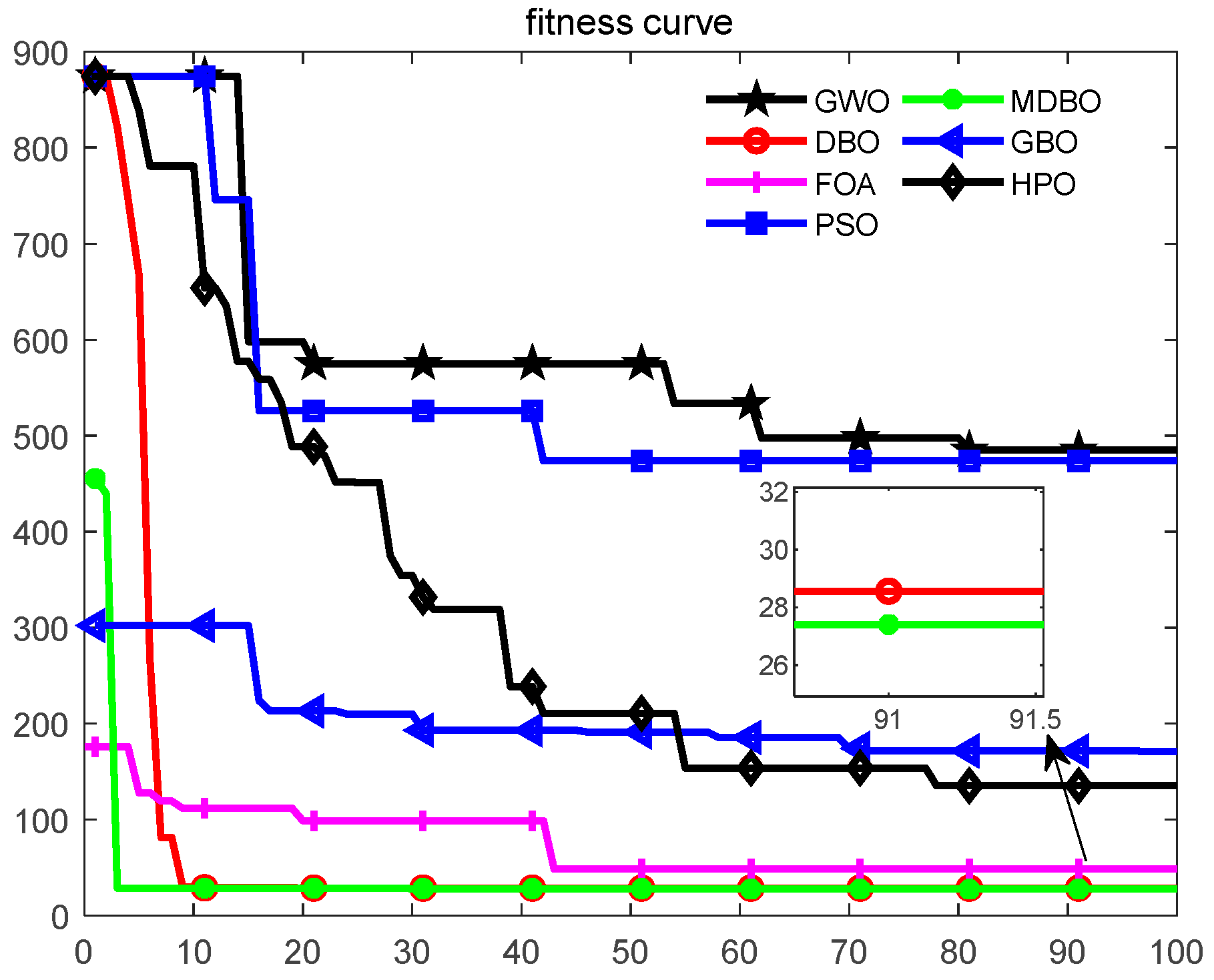
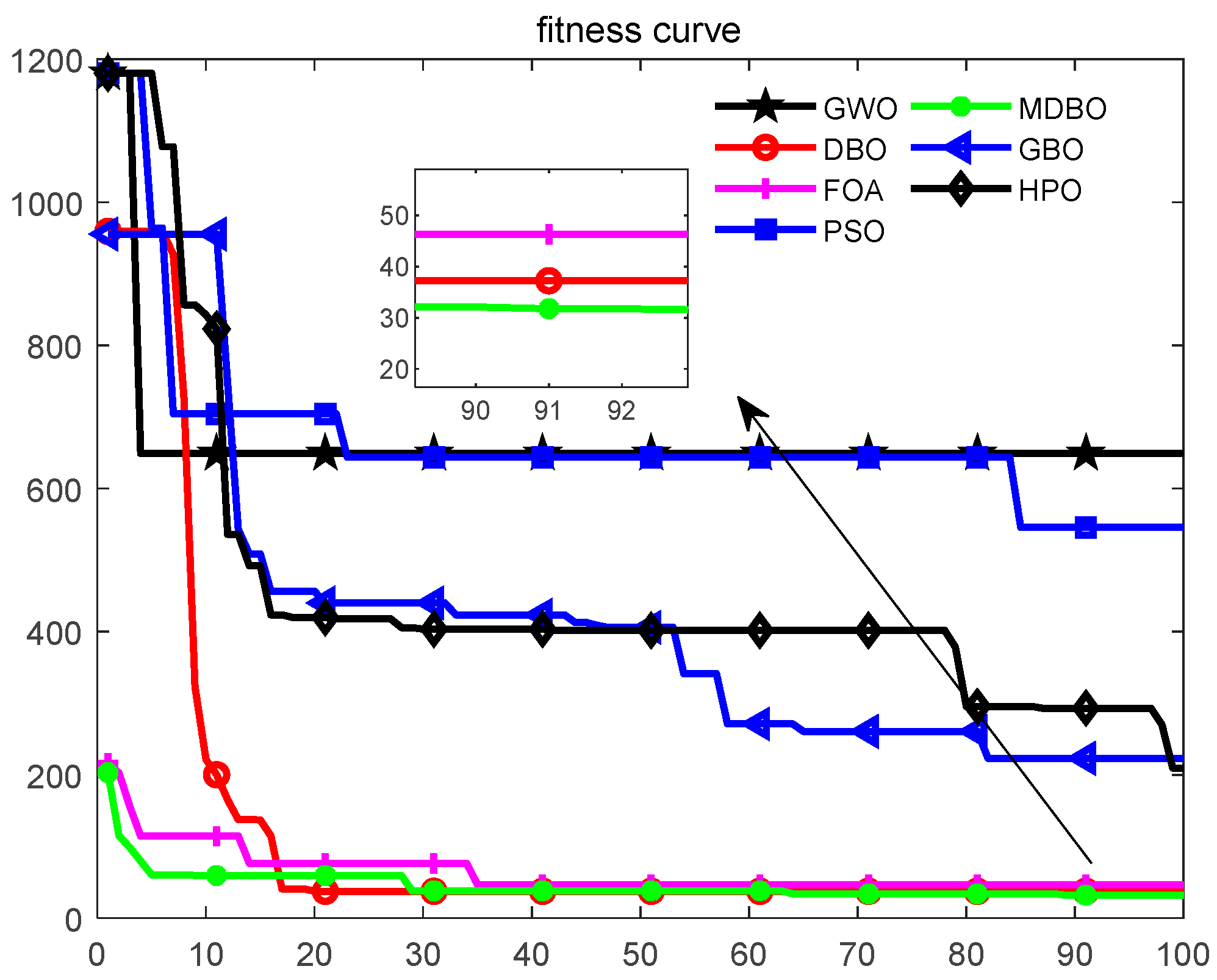
6.3. Impact of the Count and Position of Tasks

During the flight of the UAV, the task requirements need to be considered. In other words, the UAV must pass through a series of task points from the starting point and fly to the destination after completing the corresponding task. The number of task points and complexity of the task will affect the execution efficiency of the algorithm. This section mainly compares the search performance of each algorithm with different numbers of task points and coordinates. The number of set targets and their coordinates in this experiment are given in Table 6. Three groups of experiments were set up, and the number of task points in each group was 2, 3, and 4. The constant values of the cost function were the optimal weight combination according to the above experiment. The experimental results are shown in Table 7.
From Table 7, it can be intuitively observed that MDBO achieved the best results in all indices. The planned path length will also increase as the number of tasks increases. Compared with the other algorithms, it still showed a superior performance. The results indicate that MDBO can handle both simple and complex tasks. Figure 8 shows a top view of the optimal path generated by all algorithms. From Figure 8, it can be seen that all of the algorithms could successfully find secure paths. As the number of tasks increases and the complexity increases, the path will undergo significant changes. This indicates the complexity of multitasking. Meanwhile, it is evident from the comparison of paths that MDBO had smoother paths and fewer corners at task points, which means that it had a stronger optimization performance than the other algorithms.

6.4. Influence of the Number and Arrangement of Obstacles

The number and arrangement of obstacles in the map will affect the algorithm’s efficiency in finding the optimal solution. Moreover, the number of iterations required may increase if there are many obstacles in the presence of a line of sight path between the start and the destination of the UAV. Based on the previous experiments, this section assessed the performance of seven algorithms in different scenarios. We mainly set up three groups of map scenes. The number of obstacles distributed in each group of map scenes was 6, 13, and 19, respectively. The specific information of obstacles in Maps 1–3 including the coordinates and length, width, and height of obstacles are shown in Table A3, Table A4 and Table A5 in Appendix A.
The results of the average convergence curves for 100 iterations are plotted in Figure 9, Figure 10 and Figure 11. It can be seen that in all cases, MDBO always obtained the optimal solution compared to the other algorithms. For Map 1, DBO, GBO, FOA, and MDBO converged rapidly in the early stage and converged to the optimal value of around 50 iterations. The comparison from the final results found that MDBO had the highest solution accuracy, followed by the GBO. It was also found that MDBO converged to the optimal value very quickly at the beginning of the iteration, and the performance improvement was obvious compared to the original DBO. This proves that the proposed search strategies can accelerate the convergence speed and improve the convergence accuracy. For Map 2, it can be seen from Figure 10 that the GBO and FOA outperformed the DBO and MDBO at the beginning of the iterations. However, as the iterations began, DBO and MDBO converged quickly to a minimal value. At the same time, the GBO algorithm fell into a local optimum at a later stage. For Map 3, with more obstacles, the FOA and the MDBO performed the best, with the MDBO converging late to obtain the best accuracy.
On average, the number of iterations for MDBO to converge to the optimal value was 50. In general, MDBO still has a higher convergence accuracy and stronger robustness than the state-of-the-art metaheuristic methods.

7. Conclusions

In this paper, a multi-strategy enhanced dung beetle optimizer (MDBO) was proposed to improve the original algorithm’s performance using a reflective learning method, Levy boundary mapping processing, and two different cross-search mechanisms. The proposed MDBO was then used to successfully handle the three-dimensional route planning problem of oil and gas plants.
Tests for MDBO were conducted on 12 benchmark test functions, the Wilcoxon rank sum test, and the CEC2021 suite. The results showed that the MDBO is capable of handling a wide range of optimization problems and is competitive with some advanced metaheuristic algorithms. Second, based on the comparative experiments of UAV path-planning scenarios, the proposed method significantly outperformed other algorithms and achieved satisfactory results in UAV path planning. Finally, the time complexity analysis showed that the proposed MDBO increased in time complexity, so future research will focus on reducing the complexity of the algorithm. In addition, when solving the UAV path-planning problem, the UAVs are required to respond promptly when the mission dynamics change, and the number of UAVs needs to be increased if necessary, which is a limitation of this study.
Future work will focus on multi-UAV cooperation path planning in complex environments. We will also work further on reducing the running time of MDBO and applying it to more complicated optimization problems.

8. Discussion

This study provides a solution for path planning with an improved dung beetle optimizer (MDBO). It was found that the three proposed strategies effectively improved the performance of the original DBO, enabling it to solve various optimization problems. Simulation experiments in the UAV path-planning scenario demonstrated the superiority of the MDBO for path searching.
This paper examined the performance of metaheuristic algorithms such as the dung beetle optimization algorithm in solving various types of optimization problems, with a focus on the MDBO’s performance in addressing path-planning problems. First, tests were performed on 12 benchmark functions, the Wilcoxon rank sum test, and the CEC2021 suite. The results show that the three enhancement strategies can improve the original DBO’s performance and expand the algorithm’s application capabilities. This helps to verify that different improvement strategies can improve the performance of the original algorithm [23,24] and help achieve satisfactory results for specific engineering issues [22,25,26].
Second, tests on trajectory planning scenarios indicate that the DBO and the MDBO outperformed other advanced comparison algorithms. The results demonstrate the efficiency of the intelligence algorithms in solving path-planning problems [15,20,21]. In contrast to previous research, we focused on the flaws of the intelligent algorithm and aimed to develop a more reasonable search mechanism that is suitable for resolving path optimization problems.
While the findings are not surprising, it is important to understand the question of the performance gaps of the metaheuristic algorithm when applied to engineering problems. This study demonstrates the power of metaheuristic algorithms for a wide range of optimization problems and successful route planning in oil and gas plants provides theoretical support for practical navigation. However, considering the complex application environment of the real world, there will be many dynamic obstacles and changing tasks, which may require multiple UAVs to avoid dynamic obstacles. Therefore, further investigation will be considered with dynamic tasks. We will focus on designing a multi-objective beetle optimization algorithm to optimize the three-dimensional spatial navigation of several UAVs.

Author Contributions

Conceptualization, methodology, writing—original draft, software, writing—review, Q.S.; writing–review, editing, supervision, investigation, M.X.; writing–review, editing, investigation, D.Z.; writing–review, visualization, supervision, funding acquisition, Q.H. All authors have read and agreed to the published version of the manuscript.

Funding

This research was funded by National Natural Science Foundation of China, grant number No.62062021, 61872034, 62166006; Natural Science Foundation of Guizhou Province, grant number [2020]1Y254; Guizhou Provincial Science and Technology Projects, grant number Guizhou Science Foundation-ZK [2021] General 335.

Data Availability Statement

Not applicable.

Conflicts of Interest

The authors declare no conflict of interest.

Appendix A

Table A1. Twelve benchmark functions.
No.Function NameSearch SpaceDimfmin
F1Sphere[−100,100]30/50/1000
F2Schwefel 2.22[−10,10]30/50/1000
F3Schwefel 1.2[−100,100]30/50/1000
F4Schwefel 2.21[−100,100]30/50/1000
F5Zakharov[−5,10]30/50/1000
F6Step[−100,100]30/50/1000
F7Quartic[−1.28,1.28]30/50/1000
F8Qing[−500,500]30/50/1000
F9Rastrigin[−5.12,5.12]30/50/1000
F10Ackley 1[−32,32]30/50/1000
F11Griewank[−600,600]30/50/1000
F12Penalized 1[−50,50]30/50/1000
Table A2. Summary of the CEC2021 test suite [32].
No.FunctionsFi*
Unimodal FunctionCEC-1Shifted and Rotated Bent Cigar Function100
Basic FunctionsCEC-2Shifted and Rotated Schwefel’s Function1100
CEC-3Shifted and Rotated Lunacek bi-Rastrigin Function700
CEC-4Expand Rosenbrock’s plus Griewangk’s Function1900
Hybrid FunctionsCEC-5Hybrid Function 1 (N = 3)1700
CEC-6Hybrid Function 2 (N = 4)1600
CEC-7Hybrid Function 3 (N = 5)2100
Composition FunctionsCEC-8Composition Function 1 (N = 3)2200
CEC-9Composition Function 2 (N = 4)2400
CEC-10Composition Function 3 (N = 5)2500
Search range: [−100,100]D
Table A3. The data of obstacles on Map 1.
No.XYZLWH
155010005010010
2040005020010
330032005038015
480015005010015
550035005010010
65080005010010
Table A4. The data of obstacles on Map 2.
No.XYZLWH
14010001001505
245035005010010
3850100010010020
4040005020010
510040005020010
6260430010018015
760032005038015
880050005010015
943065005010010
102090005010010
1150080005010010
1245020005010010
1375020005010010
Table A5. The data of obstacles on Map 3.
No.XYZLWH
14010001001505
240015005010010
355010005010010
4850100010010020
5040005020010
610040005020010
7260430010018015
850032005010010
960032005038015
10700300010010010
1180050005010015
1230070005010010
1343065005010010
142090005010010
1510080005010010
1620080005010010
1750080005010010
1875075005010010
1990090005010010

References

  1. Jordan, S.; Moore, J.; Hovet, S.; Box, J.; Perry, J.; Kirsche, K.; Lewis, D.; Tse, Z.T.H. State-of-the-art technologies for UAV inspections. IET Radar Sonar Navig. 2018, 12, 151–164. [Google Scholar] [CrossRef]
  2. Hu, H.; Xiong, K.; Qu, G.; Ni, Q.; Fan, P.; Ben Letaief, K. AoI-Minimal Trajectory Planning and Data Collection in UAV-Assisted Wireless Powered IoT Networks. IEEE Internet Things J. 2021, 8, 1211–1223. [Google Scholar] [CrossRef]
  3. Yu, X.; Li, C.; Yen, G.G. A knee-guided differential evolution algorithm for unmanned aerial vehicle path planning in disaster management. Appl. Soft Comput. 2020, 98, 106857. [Google Scholar] [CrossRef]
  4. Lin, L.; Goodrich, M.A. UAV intelligent path planning for Wilderness Search and Rescue. In Proceedings of the 2009 IEEE/RSJ International Conference on Intelligent Robots and Systems, St. Louis, MO, USA, 10–15 October 2009; pp. 709–714. [Google Scholar] [CrossRef] [Green Version]
  5. Shin, Y.; Kim, E. Hybrid path planning using positioning risk and artificial potential fields. Aerosp. Sci. Technol. 2021, 112, 106640. [Google Scholar] [CrossRef]
  6. Huang, S.-K.; Wang, W.-J.; Sun, C.-H. A Path Planning Strategy for Multi-Robot Moving with Path-Priority Order Based on a Generalized Voronoi Diagram. Appl. Sci. 2021, 11, 9650. [Google Scholar] [CrossRef]
  7. Wang, J.; Li, Y.; Li, R.; Chen, H.; Chu, K. Trajectory planning for UAV navigation in dynamic environments with matrix alignment Dijkstra. Soft Comput. 2022, 26, 12599–12610. [Google Scholar] [CrossRef]
  8. Zhang, Z.; Wu, J.; Dai, J.; He, C. A Novel Real-Time Penetration Path Planning Algorithm for Stealth UAV in 3D Complex Dynamic Environment. IEEE Access 2020, 8, 122757–122771. [Google Scholar] [CrossRef]
  9. Lu, L.; Zong, C.; Lei, X.; Chen, B.; Zhao, P. Fixed-Wing UAV Path Planning in a Dynamic Environment via Dynamic RRT Algorithm. Mech. Mach. Sci. 2017, 408, 271–282. [Google Scholar] [CrossRef]
  10. Liu, Y.; Zheng, Z.; Qin, F.; Zhang, X.; Yao, H. A residual convolutional neural network based approach for real-time path planning. Knowl.-Based Syst. 2022, 242, 108400. [Google Scholar] [CrossRef]
  11. Chai, X.; Zheng, Z.; Xiao, J.; Yan, L.; Qu, B.; Wen, P.; Wang, H.; Zhou, Y.; Sun, H. Multi-strategy fusion differential evolution algorithm for UAV path planning in complex environment. Aerosp. Sci. Technol. 2021, 121, 107287. [Google Scholar] [CrossRef]
  12. Pehlivanoglu, Y.V.; Pehlivanoglu, P. An enhanced genetic algorithm for path planning of autonomous UAV in target coverage problems. Appl. Soft Comput. 2021, 112, 107796. [Google Scholar] [CrossRef]
  13. Phung, M.D.; Ha, Q.P. Safety-enhanced UAV path planning with spherical vector-based particle swarm optimization. Appl. Soft Comput. 2021, 107, 107376. [Google Scholar] [CrossRef]
  14. Ali, Z.A.; Han, Z.; Hang, W.B. Cooperative Path Planning of Multiple UAVs by using Max–Min Ant Colony Optimization along with Cauchy Mutant Operator. Fluct. Noise Lett. 2021, 20, 2150002. [Google Scholar] [CrossRef]
  15. Yu, X.; Li, C.; Zhou, J. A constrained differential evolution algorithm to solve UAV path planning in disaster scenarios. Knowl.-Based Syst. 2020, 204, 106209. [Google Scholar] [CrossRef]
  16. Zhang, X.; Lu, X.; Jia, S.; Li, X. A novel phase angle-encoded fruit fly optimization algorithm with mutation adaptation mechanism applied to UAV path planning. Appl. Soft Comput. 2018, 70, 371–388. [Google Scholar] [CrossRef]
  17. Dewangan, R.K.; Shukla, A.; Godfrey, W.W. Three dimensional path planning using Grey wolf optimizer for UAVs. Appl. Intell. 2019, 49, 2201–2217. [Google Scholar] [CrossRef]
  18. Xue, J.; Shen, B. Dung beetle optimizer: A new meta-heuristic algorithm for global optimization. J. Supercomput. 2022, 79, 7305–7336. [Google Scholar] [CrossRef]
  19. Peres, F.; Castelli, M. Combinatorial Optimization Problems and Metaheuristics: Review, Challenges, Design, and Development. Appl. Sci. 2021, 11, 6449. [Google Scholar] [CrossRef]
  20. Jain, G.; Yadav, G.; Prakash, D.; Shukla, A.; Tiwari, R. MVO-based path planning scheme with coordination of UAVs in 3-D environment. J. Comput. Sci. 2019, 37, 101016. [Google Scholar] [CrossRef]
  21. Li, K.; Ge, F.; Han, Y.; Wang, Y.A.; Xu, W. Path planning of multiple UAVs with online changing tasks by an ORPFOA algorithm. Eng. Appl. Artif. Intell. 2020, 94, 103807. [Google Scholar] [CrossRef]
  22. Zhang, X.; Xu, Y.; Yu, C.; Heidari, A.A.; Li, S.; Chen, H.; Li, C. Gaussian mutational chaotic fruit fly-built optimization and feature selection. Expert Syst. Appl. 2020, 141, 112976. [Google Scholar] [CrossRef]
  23. Song, S.; Wang, P.; Heidari, A.A.; Wang, M.; Zhao, X.; Chen, H.; He, W.; Xu, S. Dimension decided Harris hawks optimization with Gaussian mutation: Balance analysis and diversity patterns. Knowl.-Based Syst. 2021, 215, 106425. [Google Scholar] [CrossRef]
  24. Gupta, S.; Deep, K. A novel Random Walk Grey Wolf Optimizer. Swarm Evol. Comput. 2019, 44, 101–112. [Google Scholar] [CrossRef]
  25. Pichai, S.; Sunat, K.; Chiewchanwattana, S. An Asymmetric Chaotic Competitive Swarm Optimization Algorithm for Feature Selection in High-Dimensional Data. Symmetry 2020, 12, 1782. [Google Scholar] [CrossRef]
  26. Mikhalev, A.S.; Tynchenko, V.S.; Nelyub, V.A.; Lugovaya, N.M.; Baranov, V.A.; Kukartsev, V.V.; Sergienko, R.B.; Kurashkin, S.O. The Orb-Weaving Spider Algorithm for Training of Recurrent Neural Networks. Symmetry 2022, 14, 2036. [Google Scholar] [CrossRef]
  27. Almotairi, K.H.; Abualigah, L. Hybrid Reptile Search Algorithm and Remora Optimization Algorithm for Optimization Tasks and Data Clustering. Symmetry 2022, 14, 458. [Google Scholar] [CrossRef]
  28. Meng, A.-B.; Chen, Y.-C.; Yin, H.; Chen, S.-Z. Crisscross optimization algorithm and its application. Knowl.-Based Syst. 2014, 67, 218–229. [Google Scholar] [CrossRef]
  29. Yao, X.; Liu, Y.; Lin, G. Evolutionary programming made faster. IEEE Trans. Evol. Comput. 1999, 3, 82–102. [Google Scholar] [CrossRef] [Green Version]
  30. Cai, L.; Qu, S.; Cheng, G. Two-archive method for aggregation-based many-objective optimization. Inf. Sci. 2018, 422, 305–317. [Google Scholar] [CrossRef]
  31. Mohammadi-Balani, A.; Nayeri, M.D.; Azar, A.; Taghizadeh-Yazdi, M. Golden eagle optimizer: A nature-inspired metaheuristic algorithm. Comput. Ind. Eng. 2021, 152, 107050. [Google Scholar] [CrossRef]
  32. Mohamed, A.W.; Sallam, K.M.; Agrawal, P.; Hadi, A.A.; Mohamed, A.K. Evaluating the performance of meta-heuristic algorithms on CEC 2021 benchmark problems. Neural Comput. Appl. 2023, 35, 1493–1517. [Google Scholar] [CrossRef]
  33. Trojovský, P.; Dehghani, M. Pelican Optimization Algorithm: A Novel Nature-Inspired Algorithm for Engineering Applications. Sensors 2022, 22, 855. [Google Scholar] [CrossRef] [PubMed]
  34. Seyyedabbasi, A.; Kiani, F. Sand Cat swarm optimization: A nature-inspired algorithm to solve global optimization problems. Eng. Comput. 2022, 1–25. [Google Scholar] [CrossRef]
  35. Hashim, F.A.; Houssein, E.H.; Hussain, K.; Mabrouk, M.S.; Al-Atabany, W. Honey Badger Algorithm: New metaheuristic algorithm for solving optimization problems. Math. Comput. Simul. 2022, 192, 84–110. [Google Scholar] [CrossRef]
  36. Hegazy, A.E.; Makhlouf, M.A.; El-Tawel, G.S. Improved salp swarm algorithm for feature selection. J. King Saud Univ.—Comput. Inf. Sci. 2020, 32, 335–344. [Google Scholar] [CrossRef]
  37. Derrac, J.; García, S.; Molina, D.; Herrera, F. A practical tutorial on the use of nonparametric statistical tests as a methodology for comparing evolutionary and swarm intelligence algorithms. Swarm Evol. Comput. 2011, 1, 3–18. [Google Scholar] [CrossRef]
  38. Kennedy, J.; Eberhart, R. Particle swarm optimization. In Proceedings of the ICNN’95—International Conference on Neural Networks, Perth, Australia, 27 November–1 December 1995; pp. 1942–1948. [Google Scholar]
  39. Mirjalili, S.; Mirjalili, S.M.; Lewis, A. Grey Wolf Optimizer. Adv. Eng. Softw. 2014, 69, 46–61. [Google Scholar] [CrossRef] [Green Version]
  40. Pan, W.-T. A new Fruit Fly Optimization Algorithm: Taking the financial distress model as an example. Knowl. Based Syst. 2012, 26, 69–74. [Google Scholar] [CrossRef]
  41. Ahmadianfar, I.; Bozorg-Haddad, O.; Chu, X. Gradient-based optimizer: A new metaheuristic optimization algorithm. Inf. Sci. 2020, 540, 131–159. [Google Scholar] [CrossRef]
  42. Naruei, I.; Keynia, F.; Molahosseini, A.S. Hunter–prey optimization: Algorithm and applications. Soft Comput. 2022, 26, 1279–1314. [Google Scholar] [CrossRef]
Figure 1. Probability density function image of Beta distribution.
Symmetry 15 01432 g001
Figure 2. Cross boundary method based on Levy distribution.
Symmetry 15 01432 g002
Figure 3. Flowchart of the MDBO.
Symmetry 15 01432 g003
Figure 4. Sensitivity analysis of the MDBO’s parameters. (a) CEC-1; (b) CEC-3; (c) CEC-7; (d) CEC-10.
Symmetry 15 01432 g004
Figure 5. The convergence curves by MDBO on 12 benchmark test functions.
Symmetry 15 01432 g005aSymmetry 15 01432 g005b
Figure 6. The environment model of oil and gas plants.
Symmetry 15 01432 g006
Figure 7. Turning angle and climbing angle calculation.
Symmetry 15 01432 g007
Figure 8. The UAV paths of all algorithms under a different number of targets. (a) The generated paths when the number of tasks was 2. (b) The generated paths when the number of tasks was 3. (c) The generated paths when the number of tasks was 4.
Symmetry 15 01432 g008
Figure 9. Avg. best cost vs. iteration for Map 1.
Symmetry 15 01432 g009
Figure 10. Avg. best cost vs. iteration for Map 2.
Symmetry 15 01432 g010
Figure 11. Avg. best cost vs. iteration for Map 3.
Symmetry 15 01432 g011
Table 1. Parameter settings of all algorithms.
AlgorithmParameters
MDBOk = 0.1, b = 0.3, α = β = 0.5
POAI = 1 or 2, R = 0.2
SCSOS = 2
HBAβ = 6, C = 2
DBOk = 0.1, b = 0.3
ISSAw = 0.7
MCFOAM = 4, c1∈(0,1)
GCHHOE0∈[−1,1], θ = 0
Table 2. Twelve benchmark test function results in different dimensions.
Fun No.Name30 dim50 dim100 dim
MeanStdMeanStdMeanStd
F1DBO7.74 × 10−1143.88 × 10−1133.93 × 10−972.15 × 10−961.07 × 10−1115.84 × 10−111
POA8.32 × 10−1034.44 × 10−1021.64 × 10−998.31 × 10−999.87 × 10−1005.39 × 10−99
HBA2.58 × 10−1341.39 × 10−1331.56 × 10−1286.28 × 10−1287.48 × 10−1222.34 × 10−121
SCSO9.44 × 10−1114.99 × 10−1102.70 × 10−1091.22 × 10−1081.44 × 10−1035.79 × 10−103
GCHHO2.28 × 10−918.84 × 10−913.95 × 10−922.16 × 10−912.28 × 10−941.15 × 10−93
ISSA4.45 × 10−141.08 × 10−147.07 × 10−141.46 × 10−141.40 × 10−131.77 × 10⁻¹⁴
MCFOA6.53 × 10−111.14 × 10−101.90 × 10−103.69 × 10−107.94 × 10−101.22 × 10⁻⁹
MDBO000000
F2DBO9.65 × 10−575.28 × 10−563.97 × 10−572.18 × 10−565.75 × 10−592.40 × 10−58
POA1.11 × 10−496.05 × 10−491.92 × 10−518.90 × 10−514.73 × 10−511.71 × 10−50
HBA7.02 × 10−723.11 × 10−712.61 × 10−695.42 × 10−698.24 × 10−652.58 × 10−64
SCSO3.31 × 10−601.13 × 10−596.72 × 10−591.24 × 10−585.81 × 10−552.40 × 10−54
GCHHO2.03 × 10−471.11 × 10−463.83 × 10−491.65 × 10−486.52 × 10−482.78 × 10−47
ISSA8.83 × 10−81.34 × 10−81.46 × 10−71.64 × 10−82.97 × 10−72.15 × 10⁻⁸
MCFOA3.16 × 10−42.91 × 10−45.40 × 10−44.63 × 10−41.22 × 10−31.19 × 10⁻³
MDBO000000
F3DBO2.70 × 10−291.48 × 10−281.93 × 10−391.06 × 10−384.75 × 10−112.60 × 10⁻¹⁰
POA6.02 × 10−993.30 × 10−983.62 × 10−1001.81 × 10−996.01 × 10−982.24 × 10−97
HBA7.39 × 10−963.12 × 10−954.41 × 10−872.36 × 10−864.22 × 10−742.29 × 10−73
SCSO8.22 × 10−992.38 × 10−982.65 × 10−947.68 × 10−945.04 × 10−892.20 × 10−88
GCHHO6.90 × 10−583.35 × 10−576.52 × 10−493.55 × 10−487.71 × 10−384.22 × 10−37
ISSA4.81 × 10−135.24 × 10−131.16 × 10−121.47 × 10−124.20 × 10−123.91 × 10⁻¹²
MCFOA1.62 × 10−82.07 × 10−89.54 × 10−81.32 × 10−75.32 × 10−78.46 × 10⁻⁷
MDBO000000
F4DBO7.33 × 10−583.94 × 10−572.15 × 10−501.18 × 10−496.11 × 10−501.86 × 10−49
POA5.98 × 10−522.82 × 10−511.61 × 10−517.11 × 10−516.17 × 10−502.84 × 10−49
HBA1.53 × 10−567.64 × 10−567.69 × 10−501.86 × 10−494.23 × 10−391.71 × 10−38
SCSO3.79 × 10−511.45 × 10−504.92 × 10−491.58 × 10−481.24 × 10−475.76 × 10−47
GCHHO1.60 × 10−467.28 × 10−468.34 × 10−453.60 × 10−446.73 × 10−452.56 × 10−44
ISSA8.34 × 10−81.33 × 10−89.09 × 10−81.47 × 10−81.02 × 10−79.84 × 10⁻⁹
MCFOA3.17 × 10−63.01 × 10−66.04 × 10−67.66 × 10−68.58 × 10−66.83 × 10⁻⁶
MDBO000000
F5DBO3.13 × 10−231.70 × 10−228.97 × 10−24.91 × 10−14.91 × 1011.74 × 102
POA6.38 × 10−1033.49 × 10−1022.68 × 10−1031.44 × 10−1023.59 × 10−971.97 × 10−96
HBA8.52 × 10−613.29 × 10−601.33 × 10−247.27 × 10−243.42 × 10−41.52 × 10−3
SCSO1.67 × 10−926.08 × 10−921.05 × 10−865.00 × 10−861.09 × 10−725.90 × 10−72
GCHHO1.26 × 10−336.88 × 10−335.00 × 10−292.69 × 10−281.92 × 10−51.05 × 10−4
ISSA5.35 × 10−151.64 × 10−141.32 × 10−143.03 × 10−144.18 × 10−141.10 × 10⁻¹³
MCFOA9.13 × 10−61.01 × 10−58.72 × 10−59.45 × 10−51.09 × 10−31.71 × 10⁻³
MDBO000000
F6DBO9.15 × 10−34.53 × 10−22.97 × 10−12.69 × 10−14.68 × 1007.99 × 10−1
POA2.78 × 1005.92 × 10−15.59 × 1008.21 × 10−11.46 × 1011.08 × 100
HBA8.62 × 10−34.56 × 10−28.89 × 10−13.71 × 10−18.27 × 1009.39 × 10−1
SCSO2.06 × 1005.98 × 10−14.93 × 1007.74 × 10−11.43 × 1011.34 × 100
GCHHO7.08 × 10−76.46 × 10−71.65 × 10−51.12 × 10−52.50 × 10−41.61 × 10⁻⁴
ISSA3.03 × 1004.35 × 10−17.19 × 1006.75 × 10−11.87 × 1018.98 × 10−1
MCFOA6.75 × 1009.29 × 10−21.12 × 1011.66 × 10−12.26 × 1012.59 × 10−1
MDBO000000
F7DBO1.04 × 10−36.94 × 10−41.21 × 10−31.01 × 10−31.59 × 10−31.02 × 10⁻³
POA2.26 × 10−41.62 × 10−41.97 × 10−41.42 × 10−41.56 × 10−48.67 × 10⁻⁵
HBA3.02 × 10−41.99 × 10−43.91 × 10−43.25 × 10−45.31 × 10−44.21 × 10⁻⁴
SCSO8.98 × 10−58.64 × 10−51.79 × 10−43.71 × 10−42.29 × 10−42.99 × 10⁻⁴
GCHHO2.90 × 10−42.73 × 10−42.49 × 10−42.28 × 10−44.19 × 10−43.78 × 10⁻⁴
ISSA9.43 × 10−57.38 × 10−51.08 × 10−49.09 × 10−51.04 × 10−41.46 × 10⁻⁴
MCFOA2.15 × 10−31.54 × 10−32.61 × 10−32.80 × 10−33.73 × 10−33.52 × 10⁻³
MDBO2.81 × 10−52.13 × 10−53.04 × 10−52.18 × 10−53.50 × 10−52.40 × 10⁻⁵
F8DBO2.85 × 1011.02 × 1023.44 × 1033.74 × 1038.97 × 1042.61 × 104
POA8.65 × 1024.93 × 1026.20 × 1031.63 × 1038.63 × 1041.57 × 104
HBA2.84 × 1023.21 × 1025.67 × 1032.29 × 1031.16 × 1052.35 × 104
SCSO2.17 × 1031.05 × 1031.19 × 1043.20 × 1031.41 × 1053.39 × 104
GCHHO1.74 × 1004.61 × 1002.61 × 1012.57 × 1011.87 × 1035.35 × 102
ISSA3.18 × 1034.46 × 1021.80 × 1041.19 × 1031.73 × 1051.05 × 104
MCFOA9.36 × 1031.59 × 1024.27 × 1042.68 × 1023.37 × 1051.79 × 103
MDBO2.29 × 10−71.99 × 10−71.29 × 10−51.07 × 10−53.07 × 10−34.26 × 10⁻³
F9DBO9.96 × 10−25.45 × 10−1002.32 × 1001.27 × 101
POA000000
HBA000000
SCSO000000
GCHHO000000
ISSA000000
MCFOA4.68 × 10−68.78 × 10−68.24 × 10−61.61 × 10−52.47 × 10−53.87 × 10⁻⁵
MDBO000000
F10DBO1.01 × 10−156.49 × 10−168.88 × 10−1601.01 × 10−156.49 × 10⁻¹⁶
POA3.61 × 10−151.53 × 10−153.97 × 10−151.23 × 10−153.85 × 10−151.35 × 10⁻¹⁵
HBA6.64 × 10−13.64 × 1002.66 × 1006.89 × 1003.32 × 1007.55 × 100
SCSO8.88 × 10−1608.88 × 10−1608.88 × 10−160
GCHHO8.88 × 10−1608.88 × 10−1608.88 × 10−160
ISSA4.84 × 10−84.18 × 10−94.69 × 10−83.79 × 10−94.75 × 10−82.78 × 10⁻⁹
MCFOA1.74 × 10−51.45 × 10−51.74 × 10−51.88 × 10−51.50 × 10−51.58 × 10⁻⁵
MDBO8.88 × 10−1608.88 × 10−1608.88 × 10−160
F11DBO1.80 × 10−39.87 × 10−30000
POA000000
HBA000000
SCSO000000
GCHHO000000
ISSA9.89 × 10−144.25 × 10−141.01 × 10−134.09 × 10−141.24 × 10−133.34 × 10⁻¹⁴
MCFOA1.74 × 10−133.89 × 10−131.74 × 10−133.92 × 10−132.69 × 10−134.75 × 10⁻¹³
MDBO000000
F12DBO5.13 × 10−41.64 × 10−34.77 × 10−36.03 × 10−36.45 × 10−22.34 × 10⁻²
POA1.61 × 10−18.04 × 10−22.81 × 10−18.59 × 10−24.74 × 10−18.76 × 10⁻²
HBA4.44 × 10−41.64 × 10−31.88 × 10−28.56 × 10−31.43 × 10−15.33 × 10⁻²
SCSO9.95 × 10−24.05 × 10−22.06 × 10−15.90 × 10−23.77 × 10−17.31 × 10⁻²
GCHHO1.34 × 10−71.49 × 10−75.88 × 10−76.09 × 10−71.66 × 10−61.10 × 10⁻⁶
ISSA2.35 × 10−14.33 × 10−24.13 × 10−16.52 × 10−26.38 × 10−16.17 × 10⁻²
MCFOA1.33 × 1001.81 × 10−11.23 × 1007.90 × 10−21.13 × 1002.51 × 10−2
MDBO1.57 × 10−325.57 × 10−489.42 × 10−332.78 × 10−484.71 × 10−331.39 × 10−48
Table 3. Wilcoxon rank sum test results.
Fun No.DBOPOAHBASCSOGCHHOISSAMCFOA
p Value Rp Value Rp Value Rp Value Rp Value Rp Value Rp Value R
F11.21 × 10−121.21 × 10−121.21 × 10−121.21 × 10−121.21 × 10−121.21 × 10−121.21 × 10⁻¹²
F21.21 × 10−121.21 × 10−121.21 × 10−121.21 × 10−121.21 × 10−121.21 × 10−121.21 × 10⁻¹²
F31.21 × 10−121.21 × 10−121.21 × 10−121.21 × 10−121.21 × 10−121.21 × 10−121.21 × 10⁻¹²
F41.21 × 10−121.21 × 10−121.21 × 10−121.21 × 10−121.21 × 10−121.21 × 10−121.21 × 10⁻¹²
F51.21 × 10−121.21 × 10−121.21 × 10−121.21 × 10−121.21 × 10−121.21 × 10−121.21 × 10⁻¹²
F61.21 × 10−121.21 × 10−121.21 × 10−121.21 × 10−121.21 × 10−121.21 × 10−121.21 × 10⁻¹²
F73.02 × 10−114.08 × 10−115.07 × 10−108.88 × 10−62.83 × 10−86.55 × 10−43.34 × 10−11
F83.02 × 10−113.02 × 10−113.02 × 10−113.02 × 10−113.02 × 10−113.02 × 10−113.02 × 10⁻¹¹
F98.15 × 10−2NaNNaNNaNNaNNaN1.21 × 10−12
F10NaN8.99 × 10−111.61 × 10⁻¹NaNNaN1.21 × 10−121.21 × 10⁻¹²
F11NaNNaNNaNNaNNaN1.21 × 10−121.66 × 10⁻¹¹
F121.21 × 10−121.21 × 10−121.21 × 10−121.21 × 10−121.21 × 10−121.21 × 10−121.21 × 10⁻¹²
+/−/=9/1/210/0/210/0/29/0/39/0/311/0/112/0/0
Table 4. CEC 2021 test function results.
Fun No. DBOPOAHBASCSOGCHHOISSAMCFOAMDBO
CEC-1Mean3.62 × 1076.57 × 1095.71 × 1032.49 × 1094.20 × 1031.04 × 10105.05 × 10108.99 × 102
Std.3.47 × 1073.63 × 1094.24 × 1032.08 × 1093.42 × 1032.34 × 1096.21 × 1081.54 × 103
p-value3.02 × 10−113.02 × 10−113.08 × 1083.02 × 10−111.47 × 10−73.02 × 10−113.02 × 10⁻¹¹N/A
Signed-rank test+++++++
CEC-2Mean3.50 × 1033.12 × 1032.86 × 1033.67 × 1033.02 × 1035.79 × 1039.27 × 1031.78 × 103
Std.5.78 × 1024.21 × 1027.74 × 1024.92 × 1025.90 × 1022.99 × 1021.86 × 1022.59 × 102
p-value3.02 × 10−113.69 × 10−113.96 × 10−83.02 × 10−115.07 × 10−103.02 × 10−113.02 × 10⁻¹¹N/A
Signed-rank test+++++++
CEC-3Mean8.40 × 1029.39 × 1028.00 × 1029.06 × 1028.72 × 1029.72 × 1021.18 × 1037.58 × 102
Std.4.23 × 1012.99 × 1012.89 × 1013.52 × 1013.53 × 1013.14 × 1015.25 × 1001.34 × 101
p-value6.70 × 10−113.02 × 10−111.10 × 10−83.02 × 10−113.02 × 10−113.02 × 10−113.02 × 10⁻¹¹N/A
Signed-rank test+++++++
CEC-4Mean1.94 × 1033.51 × 1031.91 × 1033.47 × 1031.91 × 1032.15 × 1043.86 × 1071.91 × 103
Std.6.81 × 1011.78 × 1034.80 × 1003.37 × 1035.67 × 1001.48 × 1042.19 × 1064.73 × 100
p-value9.83 × 10−83.02 × 10−116.20 × 10−13.02 × 10−111.24 × 10−33.02 × 10−113.02 × 10⁻¹¹N/A
Signed-rank test++++++
CEC-5Mean1.22 × 1061.35 × 1051.64 × 1057.79 × 1054.75 × 1052.04 × 1064.81 × 1073.21 × 105
Std.9.62 × 1059.98 × 1041.21 × 1055.78 × 1052.66 × 1056.98 × 1055.83 × 1061.72 × 105
p-value3.26 × 10−75.27 × 10−54.98 × 10−43.18 × 10−41.99 × 10−23.02 × 10−113.02 × 10⁻¹¹N/A
Signed-rank test+++++++
CEC-6Mean2.24 × 1032.24 × 1032.10 × 1032.18 × 1032.00 × 1032.92 × 1037.66 × 1031.67 × 103
Std.2.53 × 1021.88 × 1023.42 × 1022.22 × 1022.01 × 1022.43 × 1021.54 × 1026.62 × 101
p-value4.08 × 10−113.34 × 10−111.96 × 10−103.34 × 10−114.50 × 10−113.02 × 10−113.02 × 10⁻¹¹N/A
Signed-rank test+++++++
CEC-7Mean6.19 × 1052.60 × 1049.52 × 1042.56 × 1051.37 × 1051.18 × 1067.69 × 1082.03 × 105
Std.7.71 × 1053.27 × 1048.49 × 1043.08 × 1059.82 × 1045.94 × 1052.63 × 1071.32 × 105
p-value1.33 × 10−25.97 × 10−96.20 × 10−46.73 × 10−15.37 × 10−29.92 × 10−113.02 × 10⁻¹¹N/A
Signed-rank test+++++
CEC-8Mean2.38 × 1033.12 × 1032.84 × 1032.93 × 1032.41 × 1033.60 × 1039.53 × 1032.51 × 103
Std.3.15 × 1028.44 × 1021.48 × 1039.68 × 1025.57 × 1026.70 × 1021.26 × 1026.20 × 102
p-value1.25 × 10−45.09 × 10−89.03 × 10−46.01 × 10−82.32 × 10−28.35 × 10−83.02 × 10−11N/A
Signed-rank test+++++++
CEC-9Mean3.00 × 1033.01 × 1032.96 × 1032.94 × 1032.94 × 1033.04 × 1034.55 × 1032.92 × 103
Std.8.21 × 1015.69 × 1011.29 × 1024.64 × 1014.87 × 1012.59 × 1011.86 × 1019.77 × 101
p-value1.11 × 10−31.09 × 10−56.52 × 10−15.30 × 10−15.49 × 10−12.92 × 10−93.02 × 10−11N/A
Signed-rank test++++
CEC-10Mean2.98 × 1033.12 × 1032.96 × 1033.07 × 1032.98 × 1033.56 × 1031.12 × 1042.99 × 103
Std.4.91 × 1011.24 × 1024.07 × 1017.76 × 1013.62 × 1011.32 × 1021.95 × 1022.24 × 101
p-value9.93 × 10−21.85 × 10−86.91 × 10−42.15 × 10−62.23 × 10−13.02 × 10−113.02 × 10⁻¹¹N/A
Signed-rank test+++=+
+/−/=/gm62/8/0/54
Table 5. Comparison of the performance of the five algorithms under different weight combinations.
W GBOHPOGWODBOFOAPSOMDBO
w1 = 0.7, w2 = 0.2, w3 = 0.1Best3.12 × 1018.01 × 1011.05 × 1023.01 × 1014.09 × 1011.81 × 1023.00 × 101
Mean6.89× 1011.78 × 1022.56 × 1023.56 × 1015.95 × 1012.68 × 1023.37 × 101
Std4.54 × 1016.03 × 1011.15 × 1025.36 × 1001.27 × 1015.65 × 1012.92 × 100
w1 = 0.2, w2 = 0.7, w3 = 0.1Best3.20 × 1011.15 × 1021.39 × 1023.56 × 1014.70 × 1011.93 × 1023.36 × 101
Mean1.08 × 1022.63 × 1022.81 × 1024.47 × 1017.91 × 1013.12 × 1024.33 × 101
Std7.53 × 1018.33 × 1011.24 × 1025.74 × 1001.38 × 1016.32 × 1015.51 × 100
w1 = 0.4, w2 = 0.4, w3 = 0.2Best3.09 × 1011.85 × 1028.88 × 1012.97 × 1014.71 × 1012.87 × 1022.80 × 101
Mean1.11 × 1023.60 × 1024.50 × 1023.59 × 1017.96 × 1014.86 × 1023.40 × 101
Std8.11 × 1011.11 × 1021.40 × 1024.77 × 1002.08 × 1018.36 × 1017.62 × 100
w1 = 0.3, w2 = 0.5, w3 = 0.2Best3.56 × 1011.66 × 1021.82 × 1023.10 × 1015.67 × 1013.53 × 1022.89 × 101
Mean1.49 × 1024.13 × 1024.41 × 1023.63 × 1019.26 × 1015.33 × 1023.47 × 101
Std8.66 × 1011.30 × 1021.64 × 1023.45 × 1002.37 × 1011.02 × 1024.39 × 100
w1 = 0.5, w2 = 0.3, w3 = 0.2Best2.99 × 1011.41 × 1021.83 × 1022.85 × 1015.86 × 1013.30 × 1022.61 × 101
Mean1.13 × 1023.14 × 1024.35 × 1023.37 × 1018.72 × 1014.81 × 1023.32 × 101
Std1.11 × 1021.05 × 1021.65 × 1027.27 × 1001.96 × 1011.04 × 1028.63 × 100
Table 6. Details of the coordinates of the tasks.
Tasks’ NumbersTarget Coordinates
2[250,650,5], [500,450,10]
3[250,650,5], [300,300,7], [700,300,10]
4[250,650,5], [300,300,7], [600,800,12], [900,400,2]
Table 7. Comparison of the performance of the five algorithms with different tasks.
Task Numbers GBOHPOGWODBOFOAPSOMDBO
2Best5.22 × 1014.58 × 1023.22 × 1025.22 × 1015.52 × 1014.96 × 1024.58 × 101
Mean1.06 × 1026.65 × 1026.00 × 1026.18 × 1016.93 × 1017.54 × 1025.50 × 101
Std7.78 × 1011.25 × 1022.10 × 1027.76 × 1007.78 × 1001.17 × 1025.02 × 100
3Best3.55 × 1013.28 × 1022.62 × 1023.61 × 1013.85 × 1014.91 × 1023.55 × 101
Mean6.58 × 1015.77 × 1024.91 × 1024.10 × 1015.90 × 1017.11 × 1023.60 × 101
Std4.60 × 1011.63 × 1022.49 × 1026.34 × 1001.24 × 1011.82 × 1027.38 × 101
4Best6.23 × 1018.01 × 1024.54 × 1028.21 × 1011.16 × 1021.05 × 1036.16 × 101
Mean1.62 × 1021.04 × 1038.55 × 1021.37 × 1021.50 × 1021.51 × 1039.73 × 101
Std8.28 × 1012.08 × 1022.18 × 1024.68 × 1012.16 × 1012.77 × 1023.28 × 101
Disclaimer/Publisher’s Note: The statements, opinions and data contained in all publications are solely those of the individual author(s) and contributor(s) and not of MDPI and/or the editor(s). MDPI and/or the editor(s) disclaim responsibility for any injury to people or property resulting from any ideas, methods, instructions or products referred to in the content.

