A New Xgamma–Weibull Model Using Type-II Adaptive Progressive Hybrid Censoring and Its Applications in Engineering and Medicine

Abstract

This paper is an attempt to study the Xgamma–Weibull distribution using an adaptive progressive type-II censoring plan. This scheme effectively ensures that the experimental time does not exceed a predetermined time limit. Using two classical estimation methods—namely, maximum likelihood and maximum product of spacing—both point and interval estimations for the unknown model parameters, as well as some parameters of life—namely, reliability and hazard rate functions—were obtained. The asymptotic normality of both classical methods was used to determine the approximate confidence intervals for the various parameters. Based on the two conventional methodologies, Bayesian estimations were also investigated using the MCMC technique under the squared error loss function. In addition, the credible intervals of the different parameters were also obtained. To compare the performance of the various approaches, a thorough simulation study was carried out. Furthermore, we propose using several optimality criteria to select the best sampling technique. Finally, two real-world datasets were used to demonstrate how the suggested estimators and optimality criteria operate in real-world circumstances.

1. Introduction

A new one-parameter Xgamma (XG$\left(\theta \right)$) distribution has been introduced by Sen et al. [1] as a special, finite mixture of exponential and gamma distributions. Recently, using the XG density, Yousof et al. [2] proposed and studied a new extension of the one-parameter Weibull distribution named the two-parameter Xgamma–Weibull (XGW$(\delta ,\theta )$) distribution. They derived several properties of the XGW distribution and also showed that its density can be represented as a mixture of exponentiated Weibull densities. Moreover, they estimated the XGW parameters using uncensored samples via the maximum likelihood estimation method. Cordeiro et al. [3] further proposed the three-parameter XGW distribution as a member of the XG family of distributions. However, we assume here that X is a lifetime random variable of an experimental unit(s) test that follows a two-parameter XGW distribution denoted by $\mathrm{XGW}\left(\mathit{\beta }\right)$, where $\mathit{\beta }={(\delta ,\theta )}^{\mathsf{T}}$ is the parameter vector. Consequently, the respective probability density function (PDF), cumulative distribution function (CDF), reliability function (RF) and hazard function (HF) for X are given, respectively, by

$$f(x;\mathit{\beta })=\frac{\theta {\delta }^2{x}^{\theta -1}{e}^{-\delta x^{\theta }}}{(1+\delta )}\left(1+\frac{1}{2}\delta x^{2\theta }\right),x>0,$$

(1)

$$F(x;\mathit{\beta })=1-\frac{e^{-\delta x^{\theta }}}{(1+\delta )}\left[1+\delta (1+x^{\theta })+\frac{1}{2}{\left(\delta x^{\theta }\right)}^2\right],$$

(2)

$$R(x;\mathit{\beta })=\frac{e^{-\delta x^{\theta }}}{(1+\delta )}\left[1+\delta (1+x^{\theta })+\frac{1}{2}{\left(\delta x^{\theta }\right)}^2\right]$$

(3)

and

$$h(x;\mathit{\beta })=\theta {\delta }^2{x}^{\theta -1}\frac{\left(1+\frac{1}{2}\delta x^{2\theta }\right)}{\left[1+\delta (1+x^{\theta })+\frac{1}{2}{\left(\delta x^{\theta }\right)}^2\right]},$$

(4)

where $\delta >0$ and $\theta >0$ are the scale and shape parameters, respectively. Using Equation (1), Yousof et al. [2] stated that the XGW distribution may be used as a generalized form of three new one-parameter lifetime distributions, which act as sub-models, namely:

• Xgamma–Rayleigh distribution if setting $\theta =2$;
• Xgamma–exponential type-I distribution if setting $\theta =1$;
• Xgamma–exponential type-II distribution if setting $\delta =1$.

Utilizing various parameter choices for $\delta$ and $\theta$ based on their domains, several shapes for density and hazard functions for the XGW distribution are shown in Figure 1. This shows that the XGW density can be concave-down or left- or right-skewed, while the XGW hazard shapes can be bathtub-shaped or decreasing or increasing.

Censored data are commonly used in studies on reliability and life testing. Due to factors like preserving working experimental units for future use, reducing overall time for the test and financial limits, investigators have to gather data using censored samples. Time-censoring (type-I) and failure-censoring (type-II) strategies are the two widely used censoring strategies in life-testing and reliability studies (see, for additional details, the work by Bain and Engelhardt [4]). These methods are not flexible enough to allow units to be removed from the experiment at any point other than the terminal point. To overcome this shortcoming, a more adaptable censoring scheme known as progressive type-II censoring has been developed. Kundu and Joarder [5] proposed a progressive type-I hybrid censoring (P-I-HC) scheme in which n identical products undergo testing via a specific progressive censoring scheme $R_1,R_2,\dots ,R_m$ and the examination terminates at an arbitrary time $T^{*}=min(X_{m:m:n},T)$, where T is a time that is predetermined. The drawback of the P-I-HC plan is that the effective sample size is random and it may be a very small number or equal to zero. As a consequence of this, statistical inference techniques will be ineffective. To address this limitation, Ng et al. [6] presented an adaptive progressive type-II hybrid censoring (AP-II-HC) strategy to improve statistical examination efficiency. In this framework, the number of failures m is specified in advance, and the duration of the test is allowed to exceed the predetermined time T. Furthermore, we have the progressive censoring scheme $R_1,R_2,\dots ,R_m$, but the values of some of the $R_i$ may change as a result of the test. This scheme can be summarized as follows: Suppose that n units are subjected to a life test and $m<n$ is the desired total number of failures. At the time of the ith failure $X_{i:m:n}$, $R_i$ units are eliminated from the test at random. If the mth failure occurs before time T (i.e., $(X_{m:m:m}<T)$), the experiment terminates and we have the regular progressive type-II censoring. If, on the other hand, $X_{d:m:n}<T<X_{d+1:m:n}$, where $d+1<m$ and $X_{d:m:n}$ correspond to the dth failure time and occur before time T, then we will not remove any living item from the experiment by placing $R_{d+1},R_{d+2},\dots ,R_{m-1}=0$ and $R_m^{*}=n-m-{\sum }_{i=1}^d{R}_i$. This setting assures that we finish the test when we attain the desired number of failures m and that the overall test duration does not deviate too much from the optimal time T. Figure 2 presents a diagrammatic representation of the AP-II-HC strategy.

Let $x_{1:m:n}<\cdots <x_{d:m:n}<T<x_{d+1:m:n}<\cdots <x_{m:m:n}$ be an AP-II-HC sample from a population with a PDF $f\left(x\right)$ and CDF $F\left(x\right)$; then, the LF for the observed data can be written according to Ng et al. [6] as

$$L=C\prod _{i=1}^{m}f\left(x_{i:m:n}\right)\prod _{i=1}^d{[1-F\left(x_{i:m:n}\right)]}^{R_i}{[1-F\left(x_{m:m:n}\right)]}^{R_m},$$

(5)

where C is a constant. Numerous studies have been conducted based on the AP-II-HC scheme; for example, the work by Al Sobhi and Soliman [7], Nassar et al. [8,9], Panahi and Moradi [10], Elshahhat and Nassar [11], Panahi and Asadi [12], Alotaibi et al. [13] and Nassar et al. [14].

A very competitive estimating technique, the maximum product of spacing estimation method, has lately acquired prominence as an alternative to the standard maximum likelihood approach. Cheng and Amin [15] initially presented the maximum product of spacing technique, demonstrating that the maximum product of spacing estimators (MPSEs) and maximum likelihood estimators (MLEs) have identical asymptotic sufficiency, consistency and efficiency features. The MPSEs are calculated by maximizing the product of the differences between the CDF values at close-ordered locations. Anatolyev and Kosenok [16] investigated the invariance property of MPSEs and discovered that it is the same as that of MLEs. The spacing function (SF) to be maximized can be written using an observed AP-II-HC sample as

$$S(\mu ,\theta )=C\prod _{i=1}^{m+1}[F\left(x_{i:m:n}\right)-F\left(x_{i-1:m:n}\right)]\prod _{i=1}^d{[1-F\left(x_{i:m:n}\right)]}^{R_i}{[1-F\left(x_{m:m:n}\right)]}^{R_m}.$$

(6)

Among others, Basu et al. [17,18], Nassar et al. [19] and Okasha and Nassar [20] have all used the maximum product of spacing estimation approach to estimate the unknown parameters of several lifetime distributions.

Though the XGW distribution is very useful in reliability analysis because its hazard shapes can be bathtub-shaped or decreasing or increasing, the problem of estimating the XGW parameters and/or the reliability and hazard rate parameters in the presence of incomplete data, such as the proposed censored sampling, has yet to be investigated. Therefore, the impetus for this study stemmed from (i) the XGW distributions’ applicability to modeling various data types with varying HRFs; (ii) the AP-II-HC scheme’s capacity to improve the accuracy of statistical estimates; and (iii) the fact that statistical and reliability scientists are interested in the performance of various estimation methods for unknown parameters, as well as the reliability and hazard rate functions of the XGW distribution. Our research objectives were as follows:

• Derive and explore the MLEs and MPSEs of unknown parameters, as well as the reliability metrics and accompanying approximate confidence intervals (ACIs);
• Investigate the Bayes estimators and Bayes credible intervals (BCIs) when observed data are gathered using both LFs and SFs and develop the MCMC method based on the squared error (SE) loss function;
• Carry out a full simulation examination to analyze the performance of the various estimations, as it is impossible to tell which approach theoretically generates the best estimates;
• Discuss the best progressive sampling plane for the AP-II-HC scheme when dealing with the XGW distribution;
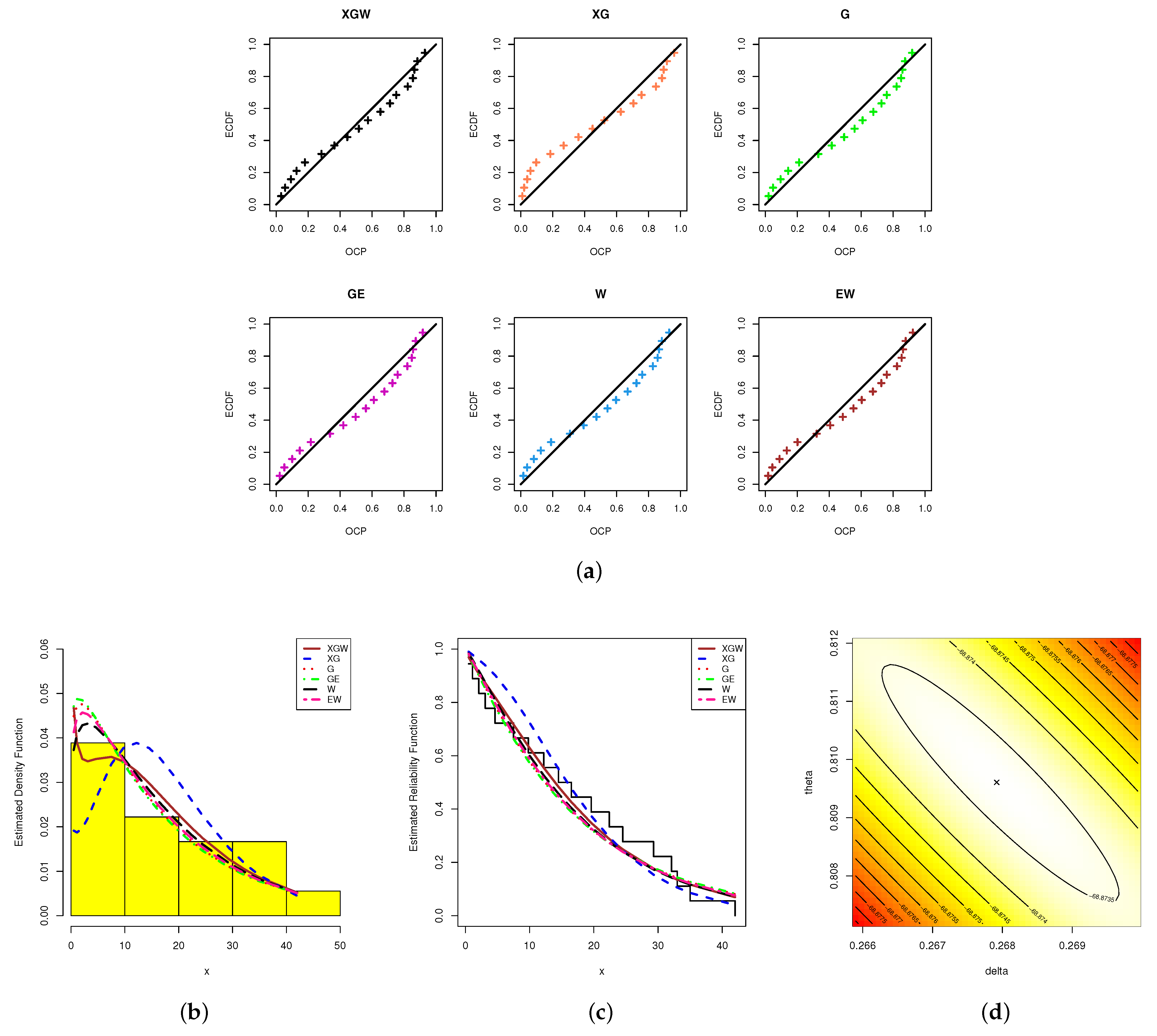
• Present two applications based on real-life engineering and medical datasets to show the superiority and flexibility of the XGW model compared to five lifetime distributions (as competitors); namely, Xgamma, gamma, generalized exponential, Weibull and exponential Weibull distributions.

The remainder of the article is organized as follows: The MLEs and the associated ACIs of the model parameters, as well as the reliability indices, are provided in Section 2. Section 3 presents the MPSEs and ACIs using the maximum product of spacing approach. Section 4 discusses Bayesian estimations using the LF and SF. Section 5 summarizes the simulation outcomes. In Section 6, optimal censoring plans based on three optimality criteria are presented. Section 7 examines two applications to real data. Finally, in Section 8, some final observations are made.

2. Likelihood Estimation

Let $x_{1:m:n}<\cdots <x_{d:m:n}<T<x_{d+1:m:n}<\cdots <x_{m:m:n}$ be an AP-II-HC sample taken from a population with a CDF, as given by Equation (2), with a progressive censoring scheme $(R_1,\dots ,R_d,0,\dots ,0,R_m)$. Then, based on Equations (1), (2) and (5), the LF, ignoring the constant term, can be written as

$$L\left(\mathit{\beta }\right|\mathit{x})=\frac{{\theta }^m{\delta }^{2m}{\left[\phi (x_m,\delta ,\theta )\right]}^{R_m}}{{(1+\delta )}^n}{e}^{-\delta \vartheta (\mathit{x},\theta )+(\theta -1){\sum }_{i=1}^{m}log\left(x_i\right)}\prod _{i=1}^m\left(1+\frac{1}{2}\delta x_i^{2\theta }\right)\prod _{i=1}^d{\left[\phi (x_i,\delta ,\theta )\right]}^{R_i},$$

(7)

where $x_i=x_{i:m:n},i=1,\dots ,m$, $\mathit{x}=(x_1,\dots ,x_m)$, $\vartheta (\mathit{x},\theta )={\sum }_{i=1}^m{x}_i^{\theta }+{\sum }_{i=1}^m{R}_i{x}_i^{\theta }+R_m{x}_m^{\theta }$ and $\phi (x_i,\delta ,\theta )=1+\delta (1+x_i^{\theta })+\frac{1}{2}{\left(\delta x_i^{\theta }\right)}^2$.

Taking the natural logarithm of Equation (7), the log-LF can be expressed as

$$\begin{array}{ccc}\hfill \ell \left(\mathit{\beta }\right|\mathit{x})& =& mlog\left(\theta \right)+2mlog\left(\delta \right)-nlog(1+\delta )-\delta \vartheta (\mathit{x},\theta )+(\theta -1){\sum }_{i=1}^{m}log\left(x_i\right)\hfill \\ & +& {\sum }_{i=1}^{m}log\left(1+\frac{1}{2}\delta x_i^{2\theta }\right)+{\sum }_{i=1}^d{R}_{i}log\left[\phi (x_i,\mathit{\beta })\right]+R_{m}log\left[\phi (x_m,\mathit{\beta })\right].\hfill \end{array}$$

(8)

By solving the following two normal equations simultaneously with respect to $\delta$ and $\theta$, one can obtain the MLEs of $\delta$ and $\theta$, denoted by $\widehat{\delta }$ and $\widehat{\theta }$, respectively, as:

$$\begin{array}{c}\hfill \frac{\partial \ell \left(\mathit{\beta }\right|\mathit{x})}{\partial \delta }=\frac{2m}{\delta }-\frac{n}{1+\delta }-\vartheta (\mathit{x},\theta )+\sum _{i=1}^m\frac{x_i^{2\theta }}{2+\delta x_i^{2\theta }}+\sum _{i=1}^d\frac{R_i{\phi }_1(x_i,\mathit{\beta })}{\phi (x_i,\mathit{\beta })}+\frac{R_m{\phi }_1(x_m,\mathit{\beta })}{\phi (x_m,\mathit{\beta })}=0\end{array}$$

(9)

and

$$\begin{array}{c}\hfill \frac{\partial \ell \left(\mathit{\beta }\right|\mathit{x})}{\partial \theta }=\frac{m}{\theta }-\delta {\vartheta }_1(\mathit{x},\theta )+\sum _{i=1}^m\frac{2\delta log\left(x_i\right)x_i^{2\theta }}{2+\delta x_i^{2\theta }}+\sum _{i=1}^d\frac{R_i{\phi }_2(x_i,\mathit{\beta })}{\phi (x_i,\mathit{\beta })}+\frac{R_m{\phi }_2(x_m,\mathit{\beta })}{\phi (x_m,\mathit{\beta })}=0,\end{array}$$

(10)

where ${\phi }_1(x_i,\mathit{\beta })=1+x_i+\delta x_i^{2\theta }$, ${\phi }_2(x_i,\mathit{\beta })={\delta }^{2}log\left(x_i\right)x_i^{2\theta }$ and ${\vartheta }_1(\mathit{x},\theta )={\sum }_{i=1}^m{x}_i^{\theta }log\left(x_i\right)+{\sum }_{i=1}^m{R}_i{x}_i^{\theta }log\left(x_i\right)+R_m{x}_m^{\theta }log\left(x_m\right)$. It is noted that the MLEs cannot be acquired from Equations (9) and (10) explicitly. Therefore, one can utilize any numerical procedure to obtain the needed estimates.

Upon obtaining the MLEs $\widehat{\delta }$ and $\widehat{\theta }$, and based on the invariance property of the MLEs, the MLEs of the RF and HRF can be derived directly from Equations (2) and (4) at mission time t, respectively, as given below

$$\widehat{R}\left(t\right)=\frac{e^{-\widehat{\delta }{t}^{\widehat{\theta }}}}{(1+\widehat{\delta })}\left[1+\widehat{\delta }(1+t^{\widehat{\theta }})+\frac{1}{2}{\left(\widehat{\delta }{t}^{\widehat{\theta }}\right)}^2\right]$$

and

$$\widehat{h}\left(t\right)=\widehat{\theta }{\widehat{\delta }}^2{t}^{\widehat{\theta }-1}\frac{\left(1+\frac{1}{2}\widehat{\delta }{t}^{2\widehat{\theta }}\right)}{\left[1+\widehat{\delta }(1+t^{\widehat{\theta }})+\frac{1}{2}{\left(\widehat{\delta }{t}^{\widehat{\theta }}\right)}^2\right]}.$$

Remark 1.

Using Equation (7), several results from the literature can be easily obtained as special cases, such as

• The estimation results presented by Sen et al. [21] in the case of the XG distribution based on progressive type-II censored sampling by setting $\theta =1$ and $T\to \infty$;
• The estimation results presented by Sen et al. [1] and Saha et al. [22] in the case of the XG distribution based on complete sampling by setting $\theta =1$, $T\to \infty$, $n=m$ and $R_i=0$ for $i=1,2,\dots ,m$;
• The estimation results presented by Elshahhat and Elemary [23] in the case of the XG distribution based on AP-II-HC sampling by setting $\theta =1$;
• The estimation results presented by Yousof et al. [2] in the case of the XGW distribution by setting $T\to \infty$, $n=m$ and $R_i=0$ for $i=1,2,\dots ,m$.

Regarding the interval estimation of the unknown parameters, as well as the RF and HRF, we employ the asymptotic properties of the MLEs to construct the ACIs of various parameters. We first use the observed Fisher information matrix to estimate the variance-covariance matrix, which is expressed as ${\mathbf{I}}^{-1}\left(\widehat{\mathit{\beta }}\right)$ and given by

$${\mathbf{I}}^{-1}\left(\widehat{\mathit{\beta }}\right)={\left[\begin{array}{c}-{\ell }_{20}-{\ell }_{12}\\ -{\ell }_{21}-{\ell }_{02}\end{array}\right]}_{(\delta =\widehat{\delta },\theta =\widehat{\theta })}^{-1}=\left[\begin{array}{c}{\widehat{V}}_{\delta }{\widehat{C}}_{\delta \theta }\\ {\widehat{C}}_{\theta \delta }{\widehat{V}}_{\theta }\end{array}\right],$$

(11)

where

$$\begin{array}{ccc}\hfill {\ell }_{20}& =& -\frac{2m}{{\delta }^2}+\frac{n}{{(1+\delta )}^2}-\sum _{i=1}^m\frac{x_i^{4\theta }}{{(2+\delta x_i^{2\theta })}^2}+\sum _{i=1}^d\frac{R_i{\phi }_{11}(x_i,\mathit{\beta })}{{\phi }^2(x_i,\mathit{\beta })}+\frac{R_m{\phi }_{11}(x_m,\mathit{\beta })}{{\phi }^2(x_m,\mathit{\beta })},\hfill \end{array}$$

$$\begin{array}{ccc}\hfill {\ell }_{02}& =& -\frac{m}{{\theta }^2}-\delta {\vartheta }_2(\mathit{x},\theta )+\sum _{i=1}^m\frac{8\delta {log}^2\left(x_i\right)x_i^{2\theta }}{{(2+\delta x_i^{2\theta })}^2}+\sum _{i=1}^d\frac{R_i{\phi }_{22}(x_i,\mathit{\beta })}{{\phi }^2(x_i,\mathit{\beta })}+\frac{R_m{\phi }_{22}(x_m,\mathit{\beta })}{{\phi }^2(x_m,\mathit{\beta })}\hfill \end{array}$$

and

$$\begin{array}{ccc}\hfill {\ell }_{12}& =& -{\vartheta }_1(\mathit{x},\theta )+\sum _{i=1}^m\frac{4x_i^{2\theta }log\left(x_i\right)}{{(2+\delta x_i^{2\theta })}^2}+\sum _{i=1}^d\frac{R_i{\phi }_{12}(x_i,\mathit{\beta })}{{\phi }^2(x_i,\mathit{\beta })}+\frac{R_m{\phi }_{12}(x_m,\mathit{\beta })}{{\phi }^2(x_m,\mathit{\beta })},\hfill \end{array}$$

where ${\phi }_{11}(x_i,\mathit{\beta })=x_i^{2\theta }\phi (x_i,\mathit{\beta })-{\phi }_1^2(x_i,\mathit{\beta })$, ${\phi }_{22}(x_i,\mathit{\beta })={\phi }_2(x_i,\mathit{\beta })[2log\left(x_i\right)\phi (x_i,\mathit{\beta })$$-{\phi }_2(x_i,\mathit{\beta })]$, ${\vartheta }_2(\mathit{x},\theta )={\sum }_{i=1}^m{x}_i^{\theta }{log}^2\left(x_i\right)+{\sum }_{i=1}^m{R}_i{x}_i^{\theta }{log}^2\left(x_i\right)+R_m{x}_m^{\theta }{log}^2\left(x_m\right)$ and ${\phi }_{12}(x_i,\mathit{\beta })={\phi }_2(x_i,\mathit{\beta })[2\delta \phi (x_i,\mathit{\beta })-{\phi }_1(x_i,\mathit{\beta })]$.

Based on the asymptotic normality of the MLEs, one can construct the ACIs of $\delta$ and $\theta$ at the $100(1-ϵ)\%$ confidence level as follows

$$\widehat{\delta }\pm z_{ϵ/2}\sqrt{{\widehat{V}}_{\delta }}\mathrm{and}\widehat{\theta }\pm z_{ϵ/2}\sqrt{{\widehat{V}}_{\theta }},$$

where $z_{ϵ/2}$ is the upper $(ϵ/2)$th percentile point of the standard normal distribution. In order to create the ACIs for the RF and HRF, we must also establish the variances for their estimators. In our case, the delta technique is used to approximate the variances of $\widehat{R\left(t\right)}$ and $\widehat{h\left(t\right)}$ (see the work by Greene [24] for additional information). We must first obtain the quantities $R_1\left(t\right),R_2\left(t\right),h_1\left(t\right)$ and $h_2\left(t\right)$, which are the first-order derivatives of the RF and HRF with respect to $\delta$ and $\theta$, respectively, to achieve the necessary estimated variances as follows

$$R_1\left(t\right)=-\frac{\delta t^{\theta }{e}^{-\delta t^{\theta }}[4+\delta (2+t^{\theta }+t^{2\theta }+\delta t^{2\theta })]}{2(1+2\delta +{\delta }^2)},$$

(12)

$$R_2\left(t\right)=-\frac{{\delta }^2{t}^{\theta }{e}^{-\delta t^{\theta }}log\left(t\right)(2+\delta )t^{2\theta }}{2(1+\delta )},$$

(13)

$$h_1\left(t\right)=\frac{\delta \theta t^{\theta }[4+4\delta t^{\theta }+\varpi (t,\mathit{\beta })]}{t{(2+2\delta +{\delta }^2{t}^{2\theta }+2\delta t^{\theta })}^2}$$

(14)

and

$$h_2\left(t\right)=\frac{{\delta }^2{t}^{\theta -1}[4(1+\delta )+\delta t^{\theta }(4+2t^{\theta }+4\delta t^{\theta }+{\delta }^2{t}^{3\theta }+2\delta t^{2\theta })+\theta log\left(t\right)\varpi (t,\mathit{\beta })]}{{(2+2\delta +{\delta }^2{t}^{2\theta }+2\delta t^{\theta })}^2},$$

(15)

where $\varpi (t,\mathit{\beta })=4+4\delta +6\delta t^{2\theta }+4{\delta }^2{t}^{2\theta }+4{\delta }^2{t}^{3\delta }+{\delta }^3{t}^{4\theta }$.

Now, let ${\mathrm{\Psi }}_R=(R_1\left(t\right),R_2\left(t\right))$ and ${\mathrm{\Psi }}_h=(h_1\left(t\right),h_2\left(t\right))$ as evaluated at the MLEs $\widehat{\delta }$ and $\widehat{\theta }$. Then, we can obtain the approximate estimates of the variances of $\widehat{R}\left(t\right)$ and $\widehat{h}\left(t\right)$, respectively, as

$${\widehat{V}}_R\approx \left[{\mathrm{\Psi }}_R{\mathbf{I}}^{-1}\left(\widehat{\mathit{\beta }}\right){\mathrm{\Psi }}_R^{\top }\right]\mathrm{and}{\widehat{V}}_h\approx \left[{\mathrm{\Psi }}_h{\mathbf{I}}^{-1}\left(\widehat{\mathit{\beta }}\right){\mathrm{\Psi }}_h^{\top }\right].$$

(16)

Consequently, the $100(1-ϵ)\%$ ACIs of RF and HRF can be expressed as

$$\widehat{R}\left(t\right)\pm z_{ϵ/2}\sqrt{{\widehat{V}}_R},\mathrm{and}\widehat{h}\left(t\right)\pm z_{ϵ/2}\sqrt{{\widehat{V}}_h},$$

respectively.

3. Product of Spacing Estimation

Let $x_{1:m:n}<\cdots <x_{d:m:n}<T<x_{d+1:m:n}<\cdots <x_{m:m:n}$ be an AP-II-HC sample from the XGW population with a CDF as given by Equation (2). Then, from Equations (2) and (6), the SF, without the constant term, can be expressed as follows with $x_i=x_{i:m:n}$

$$S\left(\mathit{\beta }\right|\mathit{x})=\frac{{\left[\phi (x_m,\delta ,\theta )\right]}^{R_m}{e}^{-\delta {\vartheta }^{*}(\mathit{x},\theta )}}{{(1+\delta )}^{n+1}}\prod _{i=1}^{m+1}\left[e^{-\delta x_{i-1}^{\theta }}\phi (x_{i-1},\mathit{\beta })-e^{-\delta x_i^{\theta }}\phi (x_i,\mathit{\beta })\right]\prod _{i=1}^d{\left[\phi (x_i,\delta ,\theta )\right]}^{R_i},$$

(17)

where ${\vartheta }^{*}(\mathit{x},\theta )={\sum }_{i=1}^m{R}_i{x}_i^{\theta }+R_m{x}_m^{\theta }$. The natural logarithm of Equation (17) is expressed as

$$\begin{array}{ccc}\hfill s\left(\mathit{\beta }\right|\mathit{x})& =& -(n+1)log(1+\delta )-\delta {\vartheta }^{*}(\mathit{x},\theta )+\sum _{i=1}^{m+1}log\left[e^{-\delta x_{i-1}^{\theta }}\phi (x_{i-1},\mathit{\beta })-e^{-\delta x_i^{\theta }}\phi (x_i,\mathit{\beta })\right]\hfill \\ & +& \sum _{i=1}^d{R}_{i}log\left[\phi (x_i,\delta ,\theta )\right]+R_{m}log\left[\phi (x_m,\delta ,\theta )\right].\hfill \end{array}$$

(18)

The MPSEs of the parameters $\delta$ and $\theta$, denoted by $\tilde{\delta }$ and $\tilde{\theta }$, can be acquired by solving the following normal equations

$$\begin{array}{ccc}\hfill \frac{\partial s\left(\mathit{\beta }\right|\mathit{x})}{\partial \delta }& =& -\frac{n+1}{1+\delta }-{\vartheta }^{*}(\mathit{x},\theta )+\sum _{i=1}^{m+1}\frac{{\Delta }_1(x_i,\mathit{\beta })-{\Delta }_1(x_{i-1},\mathit{\beta })}{\Delta (x_{i-1},\mathit{\beta })-\Delta (x_i,\mathit{\beta })}+\sum _{i=1}^d\frac{R_i{\phi }_1(x_i,\mathit{\beta })}{\phi (x_i,\mathit{\beta })}\hfill \\ & +& \frac{R_m{\phi }_1(x_m,\mathit{\beta })}{\phi (x_m,\mathit{\beta })}=0\hfill \end{array}$$

(19)

and

$$\begin{array}{c}\hfill \frac{\partial s\left(\mathit{\beta }\right|\mathit{x})}{\partial \theta }=-\delta {\vartheta }_1^{*}(\mathit{x},\theta )+\sum _{i=1}^{m+1}\frac{{\Delta }_2(x_i,\mathit{\beta })-{\Delta }_2(x_{i-1},\mathit{\beta })}{\Delta (x_{i-1},\mathit{\beta })-\Delta (x_i,\mathit{\beta })}+\sum _{i=1}^d\frac{R_i{\phi }_2(x_i,\mathit{\beta })}{\phi (x_i,\mathit{\beta })}+\frac{R_m{\phi }_2(x_m,\mathit{\beta })}{\phi (x_m,\mathit{\beta })}=0,\end{array}$$

(20)

where $\Delta (x_i,\mathit{\beta })=e^{-\delta x_i^{\theta }}\phi (x_i,\mathit{\beta })$, ${\Delta }_1(x_i,\mathit{\beta })=0.5e^{-\delta x_i^{\theta }}[\delta x_i^{\theta }(\delta x_i^{2\theta }+2)-2]$, ${\vartheta }_1^{*}(\mathit{x},\theta )$$={\sum }_{i=1}^m{R}_i{x}_i^{\theta }log\left(x_i\right)+R_m{x}_m^{\theta }log\left(x_m\right)$ and ${\Delta }_2(x_i,\mathit{\beta })=0.5{\delta }^2{x}_i^{\theta }{e}^{-\delta x_i^{\theta }}log\left(x_i\right)(\delta x_i^{2\theta }+2)$. As in the case of the MLEs, one should utilize numerical procedures to solve Equations (19) and (20) to determine the MPSEs of $\delta$ and $\theta$. According to Cheng and Traylor [25], the MPSEs possess the same invariance property as the MLEs. Therefore, we can obtain the MPSEs of the RF and HRF using this property as follows

$$\tilde{R}\left(t\right)=\frac{e^{-\tilde{\delta }{t}^{\tilde{\theta }}}}{(1+\tilde{\delta })}\left[1+\tilde{\delta }(1+t^{\tilde{\theta }})+\frac{1}{2}{\left(\tilde{\delta }{t}^{\tilde{\theta }}\right)}^2\right]$$

and

$$\tilde{h}\left(t\right)=\tilde{\theta }{\tilde{\delta }}^2{t}^{\tilde{\theta }-1}\frac{\left(1+\frac{1}{2}\tilde{\delta }{t}^{2\tilde{\theta }}\right)}{\left[1+\tilde{\delta }(1+t^{\tilde{\theta }})+\frac{1}{2}{\left(\tilde{\delta }{t}^{\tilde{\theta }}\right)}^2\right]}.$$

Cheng and Amin [15] and Cheng and Traylor [25] stated that MPSEs have the same asymptotic properties as MLEs. As a result, we can employ these properties to obtain the ACIs of the different unknown parameters based on the MPSEs. We first estimate the variance-covariance matrix based on $\tilde{\delta }$ and $\tilde{\theta }$, denoted by ${\mathbf{I}}^{-1}\left(\tilde{\mathit{\beta }}\right)$, as follows

$${\mathbf{I}}^{-1}\left(\tilde{\mathit{\beta }}\right)={\left[\begin{array}{c}-s_{20}-s_{12}\\ -s_{21}-s_{02}\end{array}\right]}_{(\delta =\tilde{\delta },\theta =\tilde{\theta })}^{-1}=\left[\begin{array}{c}{\tilde{V}}_{\delta }{\tilde{C}}_{\delta \theta }\\ {\tilde{C}}_{\theta \delta }{\tilde{V}}_{\theta }\end{array}\right],$$

(21)

where

$$\begin{array}{ccc}\hfill s_{20}& =& \frac{n+1}{{(1+\delta )}^2}+\sum _{i=1}^{m+1}\frac{{\Delta }_{11}(x_{i-1},\mathit{\beta })-{\Delta }_{11}(x_i,\mathit{\beta })}{\Delta (x_{i-1},\mathit{\beta })-\Delta (x_i,\mathit{\beta })}-\sum _{i=1}^{m+1}\frac{{[{\Delta }_1(x_i,\mathit{\beta })-{\Delta }_1(x_{i-1},\mathit{\beta })]}^2}{{[\Delta (x_{i-1},\mathit{\beta })-\Delta (x_i,\mathit{\beta })]}^2}\hfill \\ & +& \sum _{i=1}^d\frac{R_i{\phi }_{11}(x_i,\mathit{\beta })}{{\phi }^2(x_i,\mathit{\beta })}+\frac{R_m{\phi }_{11}(x_m,\mathit{\beta })}{{\phi }^2(x_m,\mathit{\beta })},\hfill \end{array}$$

$$\begin{array}{ccc}\hfill s_{02}& =& -\delta {\vartheta }_2^{*}(\mathit{x},\theta )+\sum _{i=1}^{m+1}\frac{{\Delta }_{22}(x_{i-1},\mathit{\beta })-{\Delta }_{22}(x_i,\mathit{\beta })}{\Delta (x_{i-1},\mathit{\beta })-\Delta (x_i,\mathit{\beta })}-\sum _{i=1}^{m+1}\frac{{[{\Delta }_2(x_i,\mathit{\beta })-{\Delta }_2(x_{i-1},\mathit{\beta })]}^2}{{[\Delta (x_{i-1},\mathit{\beta })-\Delta (x_i,\mathit{\beta })]}^2}\hfill \\ & +& \sum _{i=1}^d\frac{R_i{\phi }_{22}(x_i,\mathit{\beta })}{{\phi }^2(x_i,\mathit{\beta })}+\frac{R_m{\phi }_{22}(x_m,\mathit{\beta })}{{\phi }^2(x_m,\mathit{\beta })}\hfill \end{array}$$

and

$$\begin{array}{ccc}\hfill s_{12}& =& -{\vartheta }_1^{*}(\mathit{x},\theta )-\sum _{i=1}^{m+1}\frac{[{\Delta }_1(x_i,\mathit{\beta })-{\Delta }_1(x_{i-1},\mathit{\beta })][{\Delta }_2(x_i,\mathit{\beta })-{\Delta }_2(x_{i-1},\mathit{\beta })]}{{[\Delta (x_{i-1},\mathit{\beta })-\Delta (x_i,\mathit{\beta })]}^2}\hfill \\ & +& \sum _{i=1}^{m+1}\frac{{\Delta }_{12}(x_{i-1},\mathit{\beta })-{\Delta }_{12}(x_i,\mathit{\beta })}{\Delta (x_{i-1},\mathit{\beta })-\Delta (x_i,\mathit{\beta })}+\sum _{i=1}^d\frac{R_i{\phi }_{12}(x_i,\mathit{\beta })}{{\phi }^2(x_i,\mathit{\beta })}+\frac{R_m{\phi }_{12}(x_m,\mathit{\beta })}{{\phi }^2(x_m,\mathit{\beta })},\hfill \end{array}$$

where ${\Delta }_{11}(x_i,\mathit{\beta })=0.5x_i^{\theta }{e}^{-\delta x_i^{\theta }}[\delta x_i^{\theta }(\delta x_i^{2\theta }-2x_i^{\theta }+2)-4]$, ${\vartheta }_2(\mathit{x},\theta )={\sum }_{i=1}^m{R}_i{x}_i^{\theta }{log}^2\left(x_i\right)+R_m{x}_m^{\theta }{log}^2\left(x_m\right)$, ${\Delta }_{22}(x_i,\mathit{\beta })=0.5{\delta }^2{x}_i^{\theta }{e}^{-\delta x_i^{\theta }}{log}^2\left(x_i\right)[\delta x_i^{\theta }(\delta x_i^{2\theta }-3x_i^{\theta }+2)-2]$ and ${\Delta }_{12}(x_i,\mathit{\beta })=0.5\delta x_i^{\theta }{e}^{-\delta x_i^{\theta }}log\left(x_i\right)[\delta x_i^{\theta }(\delta x_i^{2\theta }-3x_i^{\theta }+2)-2]$.

Now, the $100(1-ϵ)\%$ ACIs of $\delta$ and $\theta$ can be computed respectively as

$$\tilde{\delta }\pm z_{ϵ/2}\sqrt{{\tilde{V}}_{\delta }}\mathrm{and}\tilde{\theta }\pm z_{ϵ/2}\sqrt{{\tilde{V}}_{\theta }}.$$

By approximating the estimated variances of the RF and HRF using the delta method, we can obtain the $100(1-ϵ)\%$ ACIs of $R\left(t\right)$ and $h\left(t\right)$, respectively, as follows

$$\tilde{R}\left(t\right)\pm z_{ϵ/2}\sqrt{{\tilde{V}}_R},\mathrm{and}\tilde{h}\left(t\right)\pm z_{ϵ/2}\sqrt{{\tilde{V}}_h},$$

where ${\tilde{V}}_R$ and ${\tilde{V}}_h$ are evaluated at the MPSEs of $\delta$ and $\theta$ as defined in Equation (16).

4. Bayesian Estimation

In this section, we look at the Bayesian estimation approach to estimate the XGW distribution’s parameters (the RF and HRF). The point and interval estimates of the various parameters are obtained in this section using both the LF and SF. The Bayes estimates are calculated by taking into account the SE loss function and assuming that the parameters $\delta$ and $\theta$ are independent and a priori distributed as gamma distributions. The combined prior distribution of $\delta$ and $\theta$, where $\mathit{\beta }={(\delta ,\theta )}^{\mathsf{T}}$, can be expressed as follows

$$g\left(\mathit{\beta }\right)\propto {\delta }^{a-1}{\theta }^{c-1}{e}^{-b\delta -d\theta };a,b,c,d>0.$$

(22)

Here, we assume gamma priors, which adapt to the support of the XGW distribution’s parameters and are thought to be more flexible than other prior distributions. Based on the LF given by Equation (7) and the joint prior in Equation (22), one can write the joint posterior distribution of $\delta$ and $\theta$ based on the LF as

$$\begin{array}{ccc}\hfill Q\left(\mathit{\beta }\right|\mathit{x})& =& \frac{{\theta }^{m+c-1}{\delta }^{2m+a-1}{\left[\phi (x_m,\delta ,\theta )\right]}^{R_m}}{A_1{(1+\delta )}^n}{e}^{-\delta [b+\vartheta (\mathit{x},\theta )]+\theta [{\sum }_{i=1}^{m}log\left(x_i\right)-d]}\hfill \\ & \times & \prod _{i=1}^m\left(1+\frac{1}{2}\delta x_i^{2\theta }\right)\prod _{i=1}^d{\left[\phi (x_i,\delta ,\theta )\right]}^{R_i},\hfill \end{array}$$

(23)

where

$$\begin{array}{ccc}\hfill A_1& =& {\int }_0^{\infty }{\int }_0^{\infty }\frac{{\theta }^{m+c-1}{\delta }^{2m+a-1}{\left[\phi (x_m,\delta ,\theta )\right]}^{R_m}}{{(1+\delta )}^n}{e}^{-\delta [b+\vartheta (\mathit{x},\theta )]+\theta [{\sum }_{i=1}^{m}log\left(x_i\right)-d]}\hfill \\ & \times & \prod _{i=1}^m\left(1+\frac{1}{2}\delta x_i^{2\theta }\right)\prod _{i=1}^d{\left[\phi (x_i,\delta ,\theta )\right]}^{R_i}d\delta d\theta .\hfill \end{array}$$

Similarly, by combining the SF given by Equation (17) and the joint prior in Equation (22), one can write the joint posterior distribution of $\delta$ and $\theta$ using the SP as follows

$$\begin{array}{ccc}\hfill B\left(\mathit{\beta }\right|\mathit{x})& =& \frac{{\delta }^{a-1}{\theta }^{c-1}{\left[\phi (x_m,\delta ,\theta )\right]}^{R_m}{e}^{-\delta [{\vartheta }^{*}(\mathit{x},\theta )+b]-d\theta }}{A_2{(1+\delta )}^{n+1}}\prod _{i=1}^d{\left[\phi (x_i,\delta ,\theta )\right]}^{R_i}\hfill \\ & \times & \prod _{i=1}^{m+1}\left[e^{-\delta x_{i-1}^{\theta }}\phi (x_{i-1},\mathit{\beta })-e^{-\delta x_i^{\theta }}\phi (x_i,\mathit{\beta })\right],\hfill \end{array}$$

(24)

where

$$\begin{array}{ccc}\hfill A_2& =& {\int }_0^{\infty }{\int }_0^{\infty }\frac{{\delta }^{a-1}{\theta }^{c-1}{\left[\phi (x_m,\delta ,\theta )\right]}^{R_m}{e}^{-\delta [{\vartheta }^{*}(\mathit{x},\theta )+b]-d\theta }}{{(1+\delta )}^{n+1}}\prod _{i=1}^d{\left[\phi (x_i,\delta ,\theta )\right]}^{R_i}\hfill \\ & \times & \prod _{i=1}^{m+1}\left[e^{-\delta x_{i-1}^{\theta }}\phi (x_{i-1},\mathit{\beta })-e^{-\delta x_i^{\theta }}\phi (x_i,\mathit{\beta })\right]d\delta d\theta .\hfill \end{array}$$

Under the SE loss function, the Bayes estimator of any function of the unknown parameters—say, $\xi \left(\mathit{\beta }\right)$—using both posterior distributions can be derived, respectively, as follows

$$\begin{array}{ccc}\hfill {\widehat{\xi }}_B\left(\mathit{\beta }\right)& =& {\int }_0^{\infty }{\int }_0^{\infty }\xi \left(\mathit{\beta }\right)Q\left(\mathit{\beta }\right|\mathit{x})d\delta d\theta \hfill \end{array}$$

(25)

and

$$\begin{array}{ccc}\hfill {\tilde{\xi }}_B\left(\mathit{\beta }\right)& =& {\int }_0^{\infty }{\int }_0^{\infty }\xi \left(\mathit{\beta }\right)B\left(\mathit{\beta }\right|\mathit{x})d\delta d\theta .\hfill \end{array}$$

(26)

The integrals offered by Equations (25) and (26) are not available in closed forms. As a result of this, in this scenario, we must think about using the MCMC approach to generate samples from the posterior distributions and then compute the Bayes estimates for the unknown parameters, as well as the related credible intervals. To use the MCMC technique, we first need to derive the full conditional distributions of the various parameters. Based on the posterior distribution derived based on the LF as displayed in Equation (23), the full conditional distributions of $\delta$ and $\theta$ are given, respectively, by

$$\begin{array}{c}\hfill Q_1\left(\delta \right|\theta ,\mathit{x})\propto \frac{{\delta }^{2m+a-1}{\left[\phi (x_m,\delta ,\theta )\right]}^{R_m}}{{(1+\delta )}^n}{e}^{-\delta [b+\vartheta (\mathit{x},\theta \left)\right]}\prod _{i=1}^m\left(1+\frac{1}{2}\delta x_i^{2\theta }\right)\prod _{i=1}^d{\left[\phi (x_i,\delta ,\theta )\right]}^{R_i},\end{array}$$

(27)

and

$$\begin{array}{ccc}\hfill Q_2\left(\theta \right|\delta ,\mathit{x})& \propto & {\theta }^{m+c-1}{\left[\phi (x_m,\delta ,\theta )\right]}^{R_m}{e}^{-\delta \vartheta (\mathit{x},\theta )+\theta [{\sum }_{i=1}^{m}log\left(x_i\right)-d]}\prod _{i=1}^m\left(1+\frac{1}{2}\delta x_i^{2\theta }\right)\hfill \\ & \times & \prod _{i=1}^d{\left[\phi (x_i,\delta ,\theta )\right]}^{R_i}.\hfill \end{array}$$

(28)

In a similar way, we can derive the full conditional distributions of the unknown parameters $\delta$ and $\theta$ from the posterior distribution obtained based on the SF as given by Equation (24) as follows

$$\begin{array}{ccc}\hfill B_1\left(\delta \right|\theta ,\mathit{x})& =& \frac{{\delta }^{a-1}{\left[\phi (x_m,\delta ,\theta )\right]}^{R_m}{e}^{-\delta [{\vartheta }^{*}(\mathit{x},\theta )+b]}}{{(1+\delta )}^{n+1}}\prod _{i=1}^d{\left[\phi (x_i,\delta ,\theta )\right]}^{R_i}\hfill \\ & \times & \prod _{i=1}^{m+1}\left[e^{-\delta x_{i-1}^{\theta }}\phi (x_{i-1},\mathit{\beta })-e^{-\delta x_i^{\theta }}\phi (x_i,\mathit{\beta })\right],\hfill \end{array}$$

(29)

and

$$\begin{array}{ccc}\hfill B_2\left(\theta \right|\delta ,\mathit{x})& =& {\theta }^{c-1}{\left[\phi (x_m,\delta ,\theta )\right]}^{R_m}{e}^{-\delta {\vartheta }^{*}(\mathit{x},\theta )-d\theta }\prod _{i=1}^d{\left[\phi (x_i,\delta ,\theta )\right]}^{R_i}\hfill \\ & \times & \prod _{i=1}^{m+1}\left[e^{-\delta x_{i-1}^{\theta }}\phi (x_{i-1},\mathit{\beta })-e^{-\delta x_i^{\theta }}\phi (x_i,\mathit{\beta })\right]\hfill \end{array}$$

(30)

respectively.

Although the full conditional distributions derived based on both the LF and SF cannot be represented in standard forms, their graphs are equivalent to the normal distribution. Using, for example, $(\delta ,\theta )=(0.5,1.5)$, $(a,b,c,d)=(2.5,7.5,5,5)$, $(T,n,m)=(5,100,50)$ and progressive censoring $\left(1^{50}\right)$ (where $1^{50}$ means that 1 is repeated 50 times), Figure 3 shows that the full conditional distributions in Equations (27)–(30) of $\delta$ and $\theta$ behave like normal densities. Therefore, we can employ the Metropolis–Hastings (M-H) technique with a normal proposal distribution to generate random samples from these distributions in order to obtain the required estimates.

The procedures below demonstrate how to obtain the necessary samples and the required point and credible interval estimates. It is important to mention here that the following steps are evaluated based on the LF, and one can easily use the same steps to obtain the Bayes estimates using the SF, as follows

Step 1. 

Start with the first chain $j=1$;

Step 2. 

Specify the initial values $\left({\delta }^{\left(0\right)},{\theta }^{\left(0\right)}\right)=(\widehat{\delta },\widehat{\theta });$

Step 3. 

Employ Equation (27) to simulate ${\delta }^{\left(j\right)}$ with a normal proposal distribution with mean ${\delta }^{(j-1)}$ and variance ${\widehat{V}}_{\delta }$ by using the M-H algorithm;

Step 4. 

Use Equation (28) and the M-H steps to obtain ${\theta }^{\left(j\right)}$ with a normal proposal distribution with mean ${\theta }^{(j-1)}$ and variance ${\widehat{V}}_{\theta }$;

Step 5. 

Use the obtained samples to compute $R^{\left(j\right)}\left(t\right)$ and $h^{\left(j\right)}\left(t\right)$;

Step 6. 

Set $j=j+1$;

Step 7. 

Redo steps 3–6 M times to obtain

$$\left[{\mu }^{\left(1\right)},\dots ,{\mu }^{\left(M\right)}\right],$$

where $\mu =\delta ,\theta ,R\left(t\right)$ or $h\left(t\right)$;

Step 8. 

Compute the Bayes estimate of $\mu$ using the SE loss function as

$${\widehat{\mu }}_B=\frac{1}{M-M^{*}}\sum _{j=M^{*}+1}^M{\mu }^{\left(j\right)},$$

where $M^{*}$ is the burn-in period.

5. Monte Carlo Simulations

To highlight the actual behavior of the offered estimators of $\delta$, $\theta$, $R\left(t\right)$ and $h\left(t\right)$, based on 1000 AP-II-HC samples generated from the $XGW(0.5,1.5)$ distribution, extensive simulations were conducted. For the distinct time $t=0.2$, the plausible values for $R\left(t\right)$ and $h\left(t\right)$ were taken as 0.9854 and 0.1087, respectively. Various choices for T (the threshold point), n (the full sample size) and m (the effective censored size) and different censoring schemes $R_i,i=1,2,\dots ,m$ were also utilized, such as $T(=2,5)$, $n(=40,80)$ and m being determined as a failure percentage (FP) for each n as $\frac{m}{n}\times 100\%=50$ and $80\%$. Remember that, as soon as the number of failed units reached a specific value m, the experiment was stopped. Moreover, to highlight the performance of removal methods, several designs for $R_i,i=1,2,$…$,m$ were used as follows

$$\begin{array}{cc}& \mathrm{Scheme}-1:R_1=n-m,R_i=0fori\ne 1;\hfill \\ & \mathrm{Scheme}-2:R_{\frac{m}{2}}=n-m,R_i=0fori\ne \frac{m}{2};\hfill \\ & \mathrm{Scheme}-3:R_m=n-m,R_i=0fori\ne m.\hfill \end{array}$$

To obtain AP-II-HC data from the XGW model, for pre-specific values of T, n, m and $(R_1,R_2,\dots ,R_m)$, we implemented the following generation process:

Step 1: 

Simulate traditional progressive type-II censored order statistics as follows:

a.

Create ${\rho }_i,i=1,2,\dots ,m$ independent variates of size m from a uniform $U(0,1)$ distribution;

b.

Set ${\tau }_i={\rho }_i^{{\left(i+{\sum }_{j=m-i+1}^m{R}_j\right)}^{-1}},i=1,2,\dots ,m$;

c.

Obtain $u_i=1-{\tau }_m{\tau }_{m-1}\cdots {\tau }_{m-i+1}$ for $i=1,2,\dots ,m$;

d.

Obtain $X_i=F^{-1}(u_i;\delta ,\theta ),i=1,2,\dots ,m$ from Equation (2);

Step 2: 

Find d, where $X_d<T<X_{d+1}$, and ignore the other staying items $X_i,i=d+2,\dots ,m$;

Step 3: 

From ${\left[1-F\left(x_{d+1}\right)\right]}^{-1}f\left(x\right)$, obtain the first-order $X_{d+2},\dots ,X_m$ statistics.

Once the 1000 desired AP-II-HC samples were obtained, the classical point estimates (including ML and MPS estimates), as well as 95% classical interval estimates (including ACI-LF and ACI-SF estimates), were developed. To judge the performance of the proposed density priors, we considered two separate informative sets for the hyperparameters $a_i,b_i,i=1,2;$ namely:

• Prior one: $(a_1,a_2,b_1,b_2)=(2.5,7.5,5,5)$;
• Prior two: $(a_1,a_2,b_1,b_2)=(5,15,10,10)$.

Following Section 4, we repeated the MCMC procedure 12,000 times and eliminated the first 2000 times as burn-in. After collecting 10,000 MCMC samples, based on the Bayes procedures from both likelihood-based and spacings-based estimates, the Bayes and 95% credible interval estimates of $\delta$, $\theta$, $R\left(t\right)$ and $h\left(t\right)$ were obtained. Using $\mathsf{R}$ 4.2.2 software, all frequentist and Bayes evaluations were performed using the "$\mathsf{maxLik}$" (developed by Henningsen and Toomet [26]) and "$\mathsf{coda}$" (developed by Plummer et al. [27]) packages.

Specifically, the comparison between point estimates of $\delta$ (as an example) was undertaken based on the following criteria:

• Root-mean-squared error (RMSE):

  $$\mathrm{RMSE}\left(\widehat{\widehat{\delta }}\right)=\sqrt{\frac{1}{1000}{\sum }_{i=1}^{1000}{\left({\widehat{\widehat{\delta }}}^{\left(i\right)}-\delta \right)}^2},$$
• Mean relative absolute bias (MRAB):

  $$\mathrm{MRAB}\left(\widehat{\widehat{\delta }}\right)=\frac{1}{1000}{\sum }_{i=1}^{1000}\frac{1}{\delta }\left|{\widehat{\widehat{\delta }}}^{\left(i\right)}-\delta \right|,$$

  where ${\widehat{\widehat{\delta }}}^{\left(i\right)}$ is the calculated estimate of $\delta$ at ith simulated sample.

Furthermore, the comparison of the $100(1-\gamma )\%$ interval estimates of $\delta$ was undertaken based on the following criteria:

• Average confidence length (ACL):

  $${\mathrm{ACL}}_{(1-\gamma )\%}\left(\delta \right)=\frac{1}{1000}{\sum }_{i=1}^{1000}\left({\mathcal{U}}_{{\widehat{\widehat{\delta }}}^{\left(i\right)}}-{\mathcal{L}}_{{\widehat{\widehat{\delta }}}^{\left(i\right)}}\right),$$
• Coverage percentages (CPs):

  $${\mathrm{CP}}_{(1-\gamma )\%}\left(\delta \right)=\frac{1}{1000}{\sum }_{i=1}^{1000}{\mathbf{1}}_{\left({\mathcal{L}}_{{\widehat{\widehat{\delta }}}^{\left(i\right)}};{\mathcal{U}}_{{\widehat{\widehat{\delta }}}^{\left(i\right)}}\right)}\left(\delta \right),$$

  where $\mathbf{1}(·)$ is the indicator, and ($\mathcal{L}(·)$,$\mathcal{U}(·)$) denotes the two-sided asymptotic (or Bayes credible) interval estimates of $\delta$. In the same way, the simulated RMSE, MRAB, ACL and CP results for $\theta$, $R\left(t\right)$ or $h\left(t\right)$ can be easily calculated.

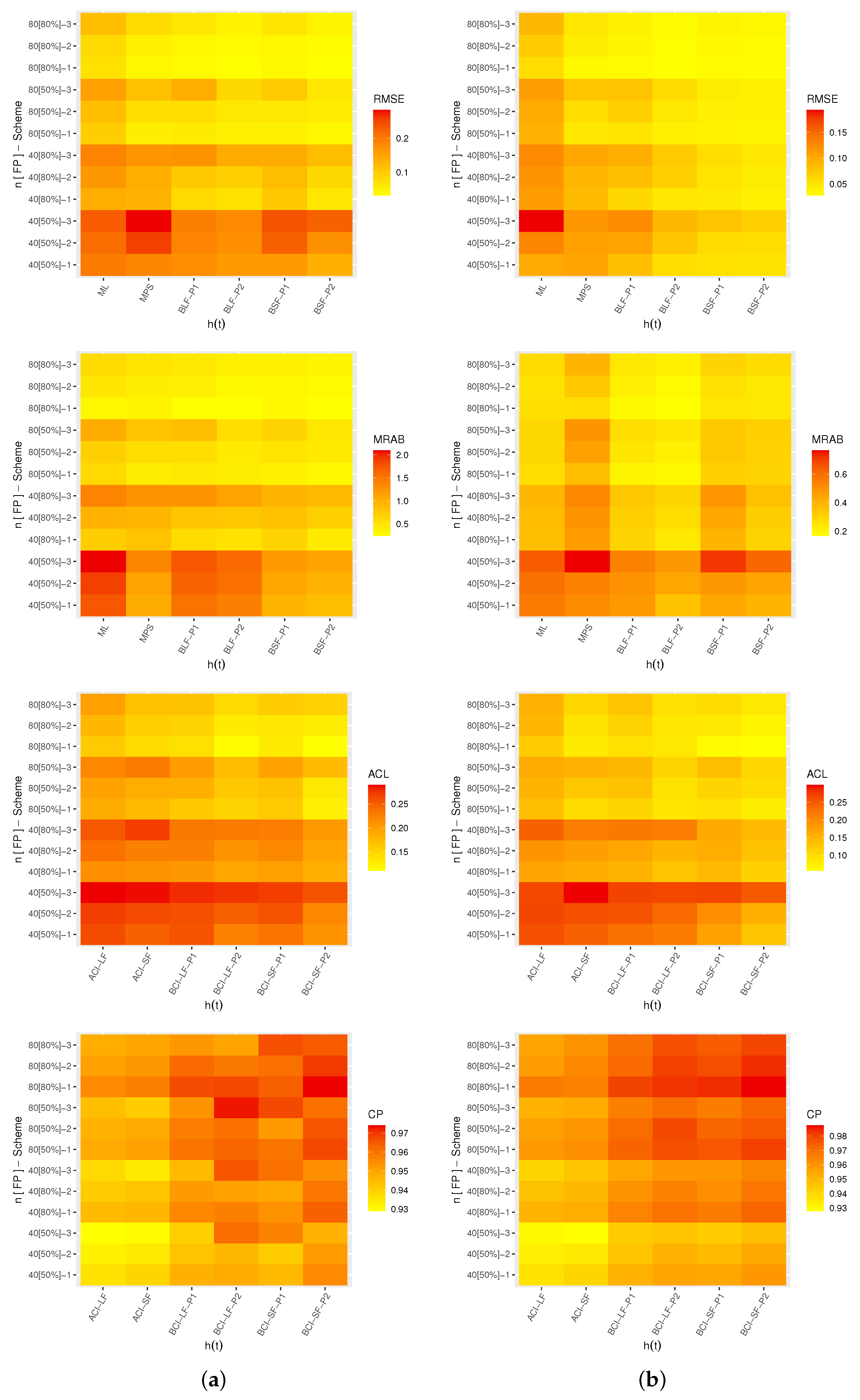
A heat map is a graphical representation of data where the individual values contained in a matrix can be represented by some specific colors. Thus, in Figure 4, Figure 5, Figure 6 and Figure 7, the simulated results for $\delta$, $\theta$, $R\left(t\right)$ and $h\left(t\right)$ are plotted, respectively. Also, all simulation tables are provided in the Supplementary File. For instance, for prior one (P1), some abbreviations are used in Figure 4, Figure 5, Figure 6 and Figure 7, such as: Bayes estimates from likelihood function (BLF-P1), Bayes estimates from spacings function (BSF-P1), Bayes credible interval from likelihood function (BCI-LF-P1) and Bayes credible interval from spacings function (BCI-SF-P1).

From Figure 4, Figure 5, Figure 6 and Figure 7, in terms of the smallest levels for the RMSEs, MRABs, ACLs and CPs, we can note the following observations:

• As a general note, when n (or m) increased, all proposed point/interval estimates performed better. A similar finding was also noted when ${\sum }_{i=1}^m{R}_i$ was narrowed down;
• As T increased, it can be seen that:

  –

  Both the RMSEs and MRABs for $\delta$ and $\theta$ increased while those associated with $R\left(t\right)$ and $h\left(t\right)$ decreased;

  –

  The ACLs for $\delta$, $R\left(t\right)$ and $h\left(t\right)$ decreased while those associated with $\theta$ decreased;

  –

  The opposite behavior was observed for all unknown parameters based on CP values;

• Comparing the proposed censoring plans, the calculated estimates of $\delta$, $\theta$, $R\left(t\right)$ and $h\left(t\right)$ were more efficient with Scheme-1 than with the others;
• Comparing the Bayesian and frequentist estimates of $\delta$, $\theta$, $R\left(t\right)$ and $h\left(t\right)$, it is clear that the point (or interval) estimates from the former were better than those obtained from the latter;
• Considering the behavior of the suggested priors, the Bayes inferences from prior two were better than those created from prior one since prior two’s variance was smaller than prior one’s;
• Comparing the proposed point estimation approaches, in most cases, the simulation results showed that:

  –

  For estimating the reliability time parameters $R\left(t\right)$ and $h\left(t\right)$, it was noted that the MPS (along with its "BSF" ) method performed better than the likelihood estimation (along with its "BLF") method;

  –

  For estimating the shape parameter $\delta$, the ML and BSF methods performed better than the others;

  –

  For estimating the scale parameter $\theta$, the MPS and BLF methods performed better than the others;

• Comparing the proposed interval estimation approaches, based on the product of spacings methodology, the simulation results showed that the interval estimates obtained from both asymptotic and credible interval methods for $\delta$, $\theta$, $R\left(t\right)$ and $h\left(t\right)$ were better than the others.

6. Optimum Progressive Censoring Plans

In earlier sections, we looked at classical and Bayesian estimations of the XGW parameters when samples were collected under AP-II-HC censoring. In a reliability context, selecting the best censoring scheme from a collection of all feasible schemes that give an extensive amount of information about the model parameter(s) of interest is an important goal for any reliability practitioner. For this objective, Balakrishnan and Aggarwala [28] first examined the topic of selecting the optimum life-testing censoring using various setups. The term "potential schemes" in this context refers to the several $(R_1,\dots ,R_m)$ choices. According to Ng et al. [29], when the values for n (total experimental units), m (effective sample size) and $(R_1,\dots ,R_m)$ (removal pattern) are prefixed in advance, one can select the optimal progressive type-II censoring design. Some prominent criteria were applied to discover the best progressive censoring scheme and are given in

Table 1. Metrics for optimum progressive plans.

Criterion	Goal
A-optimality	$\mathrm{Minimize}\mathrm{trace}({\mathrm{I}}^{-1}(\widehat{\mathit{\beta }}))$
D-optimality	$\mathrm{Minimize}det({\mathrm{I}}^{-1}(\widehat{\mathit{\beta }}))$
F-optimality	$\mathrm{Maximize}\mathrm{trace}(\mathrm{I}(\widehat{\mathit{\beta }}))$

. Table 1 shows that criteria A-optimality and D-optimality attempt to reduce the trace and determinant of the estimated variance–covariance matrices obtained based on both the LF and SF methods. Furthermore, in terms of the F-optimality criterion, we want to maximize the observed Fisher’s information values in relation to the offered MLEs (or MPSEs). The criteria in Table 1 are evaluated with the MLEs, and one can obtain them with the MPSEs by replacing the MLEs with the MPSEs.

7. Real-Life Applications

To demonstrate the significance and application of the presented approaches in real-world settings and to highlight the usefulness and flexibility of the proposed model, this section examines two real-world datasets from the engineering and medical areas.

7.1. Electronic Devices

This application involved analyzing the failure times of 18 electronic devices reported by Wang [30] and reanalyzed by Elshahhat and Abu El Azm [31]. Each data point was divided, for instance, by 10 as follows: 0.5, 1.1, 2.1, 3.1, 4.6, 7.5, 9.8, 12.2, 14.5, 16.5, 19.6, 22.4, 24.5, 29.3, 32.1, 33, 35, 42.

We first compared the XGW distribution from the complete electronic devices data with five lifetime models employing various hazard rates as their competitors; namely, the XG, gamma (G), generalized–exponential (GE), Weibull (W) and exponential–Weibull (EW) distributions. In

Table 2. Several competitors of the Xgamma–Weibull distribution.

Model	Density	Author(s)
XG$\left(\delta \right)$	${\delta }^2{(1+\delta )}^{-1}(1+\frac{1}{2}\left(\delta x^2\right))exp(-\delta x)$	Sen et al. [1]
G$(\delta ,\theta )$	$({\delta }^{\theta }/\mathrm{\Gamma }\left(\theta \right))x^{\theta -1}exp(-\delta x)$	Johnson et al. [32]
GE$(\delta ,\theta )$	$\theta \delta {(1-e^{-\delta x})}^{\theta -1}exp(-\delta x)$	Gupta and Kundu [33]
W$(\delta ,\theta )$	$\theta \delta x^{\theta -1}exp(-\delta x^{\theta })$	Weibull [34]
EW$(\delta ,\theta ,\alpha )$	$(\alpha +\delta \theta x^{\theta -1})exp(-(\alpha x+\delta x^{\theta }))$	Cordeiro et al. [35]

, all the densities of the competing models (for $x>0$ and $\delta ,\theta ,\alpha >0$), along with their author(s), are presented. To monitor the best model, six criteria for model selection were used; namely, the (1) Kolmogorov–Smirnov ($\mathsf{KS}$) (the statistic and its p-value), (2) negative-log-likelihood ($\mathsf{NL}$), (3) Akaike ($\mathsf{A}$), (4) consistent Akaike ($\mathsf{CV}$), (5) Bayesian ($\mathsf{B}$), and (6) Hannan–Quinn ($\mathsf{HB}$) measures.

Using the "$\mathsf{AdequacyModel}$" package developed by Marinho et al. [36] in $\mathsf{R}$ 4.2.2 software, the ML estimators with their standard errors (St.Es) for the model parameters, as well as the fitted criteria, were acquired (see

Table 3. Summary fit of the XGW distribution and its competitors with electronic devices.

Model	ML (St.E)			$\mathsf{NL}$	$\mathsf{A}$	$\mathsf{CA}$	$\mathsf{B}$	$\mathsf{HQ}$	$\mathsf{KS}$ (p-Value)
	$\mathit{\delta }$	$\mathit{\theta }$	$\mathit{\alpha }$
XGW	0.2678 (0.1010)	0.8097 (0.1213)	-	68.873	141.747	142.234	142.875	141.992	0.1010 (0.984)
XG	0.1529 (0.0220)	-	-	69.992	141.984	142.547	143.527	142.107	0.1808 (0.540)
G	1.1131 (0.3297)	0.0647 (0.0240)	-	69.157	142.313	143.113	144.094	142.559	0.1205 (0.929)
GE	1.0917 (0.3343)	0.0613 (0.0181)	-	69.180	142.360	143.160	144.140	142.605	0.1214 (0.925)
W	1.1451 (0.2270)	0.0371 (0.0280)	-	68.999	141.999	142.799	143.780	142.244	0.1133 (0.955)
EW	0.5307 (3.4081)	0.9892 (0.0705)	0.5710 (3.4039)	69.062	144.125	145.839	146.796	144.493	0.1177 (0.940)

). Since the XGW distribution had the smallest values with respect to the $\mathsf{NL}$, $\mathsf{A}$, $\mathsf{CA}$, $\mathsf{B}$, $\mathsf{HQ}$ and $\mathsf{KS}$ statistics, although it also had the highest p-value, Table 3 shows that the XGW distribution provided the best fit compared to all the competitor distributions. Moreover, based on the electronic devices data, we demonstrate the superiority of the proposed model via some useful plots; namely: (i) probability–probability (PP) plots; (ii) estimated PDFs; and (iii) estimated/empirical RFs (see Figure 8). From Figure 8, it can be seen that the graphical presentations support the same numerical findings as listed in Table 3. To examine the existence and uniqueness of the calculated ML estimates of the XGW parameters, the contour of the log-likelihood function for different choices of $\delta$ and $\theta$ based on the complete electronic devices dataset was also plotted and is displayed in Figure 8. It indicated that the ML estimates $\widehat{\delta }\cong 0.2678$ and $\widehat{\theta }\cong 0.8097$ existed and were unique. Henceforward, to run any additional calculations based on electronic devices data, we propose considering these values as suitable starting points.

In

Table 4. Three AP-II-HC samples from electronic devices data.

${\mathcal{S}}_{\mathit{i}}$	Scheme	$\mathit{T}\left(\mathit{d}\right)$	${\mathit{R}}_{\mathit{m}}$	Censored Items
${\mathcal{S}}_1$	$(4^2,0^8)$	30(10)	0	0.5, 1.1, 2.1, 4.6, 7.5, 9.8, 14.5, 19.6, 22.4, 29.3
${\mathcal{S}}_2$	$(0^4,4^2,0^4)$	8.5(5)	4	0.5, 1.1, 2.1, 3.1, 4.6, 9.8, 12.2, 14.5, 16.5, 19.6
${\mathcal{S}}_3$	$(0^8,4^2)$	15.5(9)	4	0.5, 1.1, 2.1, 3.1, 4.6, 7.5, 9.8, 12.2, 14.5, 16.5

, using the complete electronic devices data and based on $m=10$ with different choices for T and R, the results for different AP-II-HC samples are reported. For example, censoring scheme $(0,0,0,1,1,1)$ is denoted as $(0^3,1^3)$. For ${\mathcal{S}}_i,i=1,2,3,$ the point classical (including ML and MPS) estimates with their St.Es and 95% asymptotic interval (including ACI-LF and ACI-SF) estimates with their interval widths (IWs) were calculated and are provided in

Table 5. Estimates of $\delta$, $\theta$, $R\left(t\right)$ and $h\left(t\right)$ from electronic devices data.

Sample	Par.	ML		BLF		ACI-LF			BCI-LF
		MPS		BSF		ACI-SF			BCI-SF
		Est.	St.E	Est.	St.E	Lower	Upper	IW	Lower	Upper	IW
${\mathcal{S}}_1$	$\delta$	0.3344	0.1343	0.2746	0.0714	0.0713	0.5976	0.5263	0.2001	0.3534	0.1533
		0.2897	0.1283	0.2742	0.0418	0.0382	0.5412	0.5030	0.2000	0.3528	0.1528
	$\theta$	0.8315	0.1485	0.8867	0.0705	0.5405	1.1225	0.5820	0.8018	0.9729	0.1711
		0.9115	0.1672	0.8871	0.0501	0.5837	1.2392	0.6555	0.8014	0.9728	0.1714
	$R\left(5\right)$	0.7166	0.1093	0.7676	0.0702	0.5023	0.9309	0.4286	0.6675	0.8567	0.1892
		0.7362	0.1123	0.7679	0.0577	0.5162	0.9563	0.4400	0.6688	0.8575	0.1887
	$h\left(5\right)$	0.0711	0.0251	0.0620	0.0183	0.0218	0.1204	0.0986	0.0348	0.0969	0.0621
		0.0741	0.0279	0.0620	0.0200	0.0194	0.1287	0.1093	0.0345	0.0970	0.0625
${\mathcal{S}}_2$	$\delta$	0.3051	0.1214	0.2509	0.0652	0.0672	0.5431	0.4758	0.1841	0.3248	0.1406
		0.2795	0.1190	0.2506	0.0468	0.0462	0.5128	0.4666	0.1809	0.3273	0.1464
	$\theta$	0.7706	0.1575	0.8680	0.1069	0.4619	1.0793	0.6174	0.7836	0.9538	0.1702
		0.8133	0.1693	0.8699	0.0718	0.4814	1.1452	0.6638	0.7831	0.9556	0.1725
	$R\left(5\right)$	0.7782	0.0870	0.8054	0.0499	0.6076	0.9488	0.3412	0.7171	0.8820	0.1649
		0.7913	0.0875	0.8051	0.0445	0.6198	0.9628	0.3430	0.7182	0.8811	0.1629
	$h\left(5\right)$	0.0480	0.0162	0.0490	0.0126	0.0163	0.0797	0.0634	0.0275	0.0766	0.0491
		0.0481	0.0166	0.0492	0.0127	0.0156	0.0806	0.0650	0.0278	0.0763	0.0484
${\mathcal{S}}_3$	$\delta$	0.3134	0.1259	0.2479	0.0747	0.0665	0.5602	0.4937	0.1802	0.3218	0.1416
		0.2926	0.1254	0.2470	0.0583	0.0467	0.5384	0.4917	0.1792	0.3217	0.1425
	$\theta$	0.7418	0.1647	0.8642	0.1307	0.4190	1.0646	0.6455	0.7739	0.9521	0.1782
		0.7756	0.1771	0.8671	0.1015	0.4285	1.1228	0.6942	0.7800	0.9532	0.1732
	$R\left(5\right)$	0.7802	0.0852	0.8104	0.0505	0.6132	0.9473	0.3341	0.7256	0.8841	0.1585
		0.7904	0.0860	0.8106	0.0457	0.6218	0.9590	0.3371	0.7254	0.8859	0.1605
	$h\left(5\right)$	0.0451	0.0149	0.0472	0.0121	0.0159	0.0744	0.0584	0.0270	0.0732	0.0463
		0.0454	0.0151	0.0474	0.0122	0.0157	0.0750	0.0593	0.0267	0.0736	0.0469

. Using the M-H algorithm steps, from the proposed posterior PDFs, we simulated 50,000 MCMC iterations and discarded the first 10,000 of them. Based on the non-informative priors of $\delta$ and $\theta$, the Bayes estimates (with their St.Es) of $\delta$ and $\theta$ and $R\left(t\right)$ and $h\left(t\right)$ (at the distinct time $t=5$) were also obtained (see Table 5). Moreover, from the 40,000 MCMC variates retained, 95% asymptotic interval (including BCI-LF and BCI-SF) estimates with their IWs for the same unknown quantities were also computed and are presented in Table 5. These findings show that, with regard to the lowest levels for the St.E and IW values, the estimates created from the Bayes MCMC approach through MCMC-LF (or MCMC-SF) methods for $\delta$, $\theta$, $R\left(t\right)$ and $h\left(t\right)$ performed better than the others. A similar conclusion was also reached when the asymptotic intervals were compared with the credible intervals.

To evaluate the convergence of the 40,000 MCMC variates simulated with the LF and SF approaches, using ${\mathcal{S}}_1$ data as an example, the traces and Gaussian kernel densities are shown in Figure 9 with histogram plots of $\delta$, $\theta$, $R\left(t\right)$ and $h\left(t\right)$. In each plot, the sample mean is highlighted by a solid blue line. In each histogram, 95% BCI bounds are highlighted by dashed lines. Figure 9 indicates that the proposed MCMC samplers converged adequately. It also indicates that the generated posterior estimates of $\delta$ and $\theta$ were very close to being symmetric, while those of $R\left(t\right)$ and $h\left(t\right)$ were negatively and positively skewed, respectively. Moreover, using ${\mathcal{S}}_i,i=1,2$ datasets, the trace and histogram plots for $\delta$, $\theta$, $R\left(t\right)$ and $h\left(t\right)$ are presented in the Supplementary File for easy access.

Following the optimum criteria provided in Table 1, from the evaluated variances and covariances of the ML and MPS estimates obtained from the generated samples ${\mathcal{S}}_i,i=1,2,3$, the best progressive censoring was determined (see

Table 6. Optimum censoring from electronic devices data.

Scheme	Criterion
	A	D	F
LF approach
${\mathcal{S}}_1$	3.95$\times {10}^{-2}$	8.03$\times {10}^{-4}$	492.3706
${\mathcal{S}}_2$	4.01$\times {10}^{-2}$	9.63$\times {10}^{-4}$	417.0246
${\mathcal{S}}_3$	4.30$\times {10}^{-2}$	9.03$\times {10}^{-4}$	476.0067
SF approach
${\mathcal{S}}_1$	4.28$\times {10}^{-2}$	7.79$\times {10}^{-4}$	550.3082
${\mathcal{S}}_2$	4.44$\times {10}^{-2}$	9.76$\times {10}^{-4}$	455.4188
${\mathcal{S}}_3$	4.71$\times {10}^{-2}$	9.04$\times {10}^{-4}$	520.8349

). For both LF and SF approaches, the censoring scheme used with sample ${\mathcal{S}}_1$ was the best censoring plan for all given criteria. The optimum progressive censoring suggested in this application supported the results obtained in the simulation experiments.

7.2. Head and Neck Cancer

This application involved examining the survival periods (in days) of 44 individuals with cancer of the head and neck (CHN) (see

Table 7. Survival times of 44 CHN patients.

12.20	23.56	23.74	25.87	31.98	37	41.35	47.38	55.46	58.36
63.47	68.46	74.47	78.26	81.43	84	92	94	110	112
119	127	130	133	140	146	155	159	173	179
194	195	209	249	281	319	339	432	469	519
633	725	817	1776

). These patients were treated using a combination of radiotherapy and chemotherapy. This dataset was first published by Efron [37] and previously reanalyzed by Elshahhat and Rastogi [38].

To compare the XGW distribution with the other competitive models presented in Table 2, based on the complete CHN dataset, the evaluated values for the $\mathsf{NL}$, $\mathsf{A}$, $\mathsf{CA}$, $\mathsf{B}$, $\mathsf{HQ}$, and $\mathsf{KS}$ (p-value) statistics are reported in

Table 8. Summary fit of the XGW distribution and its competitors from CHN data.

Model	ML (St.E)			NL	A	CA	B	HQ	KS (p-Value)
	$\mathit{\delta }$	$\mathit{\theta }$	$\mathit{\alpha }$
XGW	0.1189 (0.0349)	0.6102 (0.0528)	-	281.38	566.76	567.05	570.33	568.08	0.1172 (0.542)
XG	0.0132 (0.0012)	-	-	303.38	608.77	608.86	610.55	609.43	0.2808 (0.002)
G	1.0483 (0.1881)	0.0048 (0.0010)	-	282.02	568.03	568.32	571.60	569.35	0.1439 (0.293)
GE	1.0918 (0.2222)	0.0048 (0.0009)	-	281.96	567.93	568.22	571.50	569.25	0.1457 (0.279)
W	0.9239 (0.0783)	0.0070 (0.0033)	-	281.86	567.71	568.00	571.28	569.04	0.1268 (0.442)
EW	0.0020 (0.0007)	1.1193 (0.0543)	0.0006 (0.0024)	283.17	572.34	572.94	577.69	574.32	0.1565 (0.208)

. The ML estimates (along with their St.Es) of all competing models were also computed (see Table 8). It is obvious from the complete CHN data that the XGW distribution had the highest p-value and the smallest values with respect to the other fitted criteria. Thus, the XGW distribution was the best choice compared to the others. Also, it is clear from Table 3 and Table 8 that the best competitive lifetime model close to the proposed XGW distribution was the two-parameter W lifetime model. Again, based on the CHN data, the PP plots, estimated PDF and estimated/empirical RF, as well as the contour plot of the log-likelihood function, were plotted and are displayed in Figure 10. As we anticipated, the data in Figure 10 supported the results presented in Table 8. Moreover, the data in Figure 10d showed that the ML estimates $\widehat{\delta }\cong 0.1189$ and $\widehat{\theta }\cong 0.8097$ existed and were unique.

Next, from the full CHN data, various artificial AP-II-HC samples were generated and are reported in

Table 9. Three AP-II-HC samples from CHN data.

${\mathcal{S}}_{\mathit{i}}$	Scheme	$\mathit{T}\left(\mathit{d}\right)$	${\mathit{R}}_{\mathit{m}}$	Censored Items
${\mathcal{S}}_1$	$(5^4,0^{20})$	250(24)	0	12.20, 23.56, 23.74, 25.87, 31.98, 37, 41.35, 47.38, 55.46, 58.36, 68.46,
				74.47, 78.26, 92, 94, 110, 127, 146, 155, 179, 194, 195, 209, 249
${\mathcal{S}}_2$	$(0^{10},5^4,0^{10})$	75(13)	5	12.20, 23.56, 23.74, 25.87, 31.98, 37, 41.35, 47.38, 55.46, 58.36, 63.47,
				68.46, 74.47, 78.26, 81.43, 84, 92, 94, 110, 112, 119, 127, 130, 133
${\mathcal{S}}_3$	$(0^{20},5^4)$	128(22)	10	12.20, 23.56, 23.74, 25.87, 31.98, 37, 41.35, 47.38, 55.46, 58.36, 63.47,
				68.46, 74.47, 78.26, 81.43, 84, 92, 94, 110, 112, 119, 127, 130, 133

. Using Table 9, the offered point estimates (with their St.Es) and the offered interval estimates (with their IWs) of $\delta$, $\theta$, $R\left(t\right)$ and $h\left(t\right)$ at $t=0.50$ could be calculated and are listed in

Table 10. Estimates of $\delta$, $\theta$, $R\left(t\right)$ and $h\left(t\right)$ from CHN data.

Sample	Par.	ML		BLF		ACI-LF			BCI-LF
		MPS		BSF		ACI-SF			BCI-SF
		Est.	St.E	Est.	St.E	Lower	Upper	IW	Lower	Upper	IW
${\mathcal{S}}_1$	$\delta$	0.0450	0.0214	0.0451	0.0050	0.0029	0.0870	0.0841	0.0358	0.0552	0.0194
		0.0370	0.0191	0.0365	0.0041	−0.0005	0.0744	0.0749	0.0289	0.0447	0.0158
	$\theta$	0.9075	0.1020	0.9073	0.0097	0.7077	1.1074	0.3997	0.8881	0.9265	0.0385
		0.9542	0.1107	0.9529	0.0089	0.7373	1.1710	0.4338	0.9356	0.9701	0.0345
	$R\left(50\right)$	0.7671	0.0613	0.7656	0.0436	0.6469	0.8872	0.2403	0.6762	0.8464	0.1702
		0.7768	0.0617	0.7835	0.0426	0.6559	0.8976	0.2417	0.6958	0.8597	0.1638
	$h\left(50\right)$	0.0094	0.0021	0.0095	0.0019	0.0053	0.0135	0.0083	0.0061	0.0134	0.0073
		0.0096	0.0022	0.0093	0.0019	0.0053	0.0139	0.0087	0.0060	0.0133	0.0074
${\mathcal{S}}_2$	$\delta$	0.0246	0.0154	0.0246	0.0024	−0.0056	0.0547	0.0603	0.0200	0.0295	0.0095
		0.0193	0.0132	0.0192	0.0019	−0.0065	0.0450	0.0515	0.0156	0.0230	0.0074
	$\theta$	1.0278	0.1404	1.0278	0.0049	0.7525	1.3030	0.5505	1.0180	1.0375	0.0195
		1.0832	0.1527	1.0830	0.0040	0.7839	1.3825	0.5985	1.0752	1.0908	0.0156
	$R\left(50\right)$	0.8269	0.0480	0.8255	0.0327	0.7329	0.9209	0.1880	0.7578	0.8848	0.1270
		0.8384	0.0472	0.8388	0.0309	0.7458	0.9310	0.1852	0.7732	0.8947	0.1215
	$h\left(50\right)$	0.0081	0.0018	0.0082	0.0016	0.0047	0.0116	0.0069	0.0054	0.0115	0.0061
		0.0081	0.0018	0.0081	0.0016	0.0046	0.0116	0.0070	0.0053	0.0114	0.0061
${\mathcal{S}}_3$	$\delta$	0.0415	0.0233	0.0413	0.0030	−0.0042	0.0873	0.0915	0.0355	0.0473	0.0118
		0.0473	0.0251	0.0473	0.0036	−0.0018	0.0964	0.0982	0.0404	0.0545	0.0141
	$\theta$	0.8684	0.1223	0.8682	0.0040	0.6286	1.1082	0.4796	0.8604	0.8760	0.0156
		0.8395	0.1156	0.8394	0.0049	0.6130	1.0660	0.4530	0.8297	0.8491	0.0194
	$R\left(50\right)$	0.8473	0.0461	0.8484	0.0217	0.7570	0.9376	0.1806	0.8038	0.8887	0.0849
		0.8395	0.0466	0.8392	0.0236	0.7482	0.9307	0.1825	0.7909	0.8830	0.0921
	$h\left(50\right)$	0.0057	0.0013	0.0057	0.0008	0.0033	0.0082	0.0049	0.0041	0.0074	0.0033
		0.0058	0.0012	0.0058	0.0009	0.0033	0.0082	0.0049	0.0042	0.0076	0.0034

. Just like our settings for the MCMC sampler described in Section 7.1, to perform the Bayesian calculations, we generated 40,000 MCMC variates after ignoring the first 10,000 variates.

From Table 10, it can be seen the Bayes (point/interval) estimates of $\delta$, $\theta$, $R\left(t\right)$ and $h\left(t\right)$ were quite close to the frequentist (point/interval) estimates. As an example, both trace and density plots for the 40,000 MCMC estimates of $\delta$, $\theta$, $R\left(t\right)$ and $h\left(t\right)$ based on the ${\mathcal{S}}_1$ data are displayed in Figure 11. They show that the simulated MCMC samples converged sufficiently. They also support the facts displayed in Figure 9. Additionally, the trace and histogram plots for the same parameters using the ${\mathcal{S}}_1$ and ${\mathcal{S}}_2$ datasets were also plotted and are given in the Supplementary File.

Furthermore, using all samples for ${\mathcal{S}}_i,i=1,2,3$ presented in Table 9, the best progressive censoring was determined and is provided in

Table 11. Optimum censoring from CHN data.

Scheme	Criterion
	A	D	F
LF approach
${\mathcal{S}}_1$	1.09$\times {10}^{-2}$	1.40$\times {10}^{-7}$	142,175.87
${\mathcal{S}}_2$	2.00$\times {10}^{-2}$	2.88$\times {10}^{-7}$	37,671.185
${\mathcal{S}}_3$	1.39$\times {10}^{-2}$	3.45$\times {10}^{-7}$	40,490.846
SF approach
${\mathcal{S}}_1$	1.26$\times {10}^{-2}$	2.37$\times {10}^{-7}$	229,393.37
${\mathcal{S}}_2$	2.35$\times {10}^{-2}$	3.02$\times {10}^{-7}$	53,316.811
${\mathcal{S}}_3$	1.55$\times {10}^{-2}$	2.98$\times {10}^{-7}$	52,098.656

. The progressive design used with sample ${\mathcal{S}}_1$ was the best censoring plan with respect to all the optimum criteria considered in Table 1. Table 11 also supports the findings reported in Section 5.

Ultimately, in the presence of adaptive type-II progressive hybrid censored information, we can state that the analysis of the given real datasets showed that the proposed estimation methodologies can be easily used in practical scenarios and provide a good demonstration of the XGW distribution.

8. Concluding Remarks

This paper addressed the estimation issues involving unknown parameters, reliability and hazard rate functions with the Xgamma–Weibull distribution using an adaptive progressive type-II censoring strategy. For this goal, traditional estimating methods, such as likelihood and product of spacings estimates, were applied, and then Bayesian estimates were also used based on these two methodologies. The Bayesian estimates were calculated using independent gamma priors and the squared error loss function. The asymptotic properties of the acquired frequentist estimates were used to create the asymptotic confidence intervals for all unknown quantities. In the Bayes framework, point estimates were obtained using MCMC techniques, and the credible intervals were calculated using the same methodology. A simulation study was conducted under various conditions to compare the outcomes of the various estimations. According to the simulation results, Bayesian estimates outperformed conventional estimates in terms of the root-mean-squared error, the relative absolute bias, the confidence length and the coverage percentage. Furthermore, we provided an optimal censoring strategy based on several information measures. Finally, two real-world datasets were analyzed to show how the proposed approaches can be used in practice.

References

1. Sen, S.; Maiti, S.S.; Chandra, N. The xgamma distribution: Statistical properties and application. J. Mod. Appl. Stat. Methods 2016, 15, 38. [Google Scholar] [CrossRef] [Green Version]
2. Yousof, H.M.; Korkmaz, M.Ç.; Sen, S. A new two-parameter lifetime model. Ann. Data Sci. 2021, 8, 91–106. [Google Scholar] [CrossRef]
3. Cordeiro, G.M.; Altun, E.; Korkmaz, M.C.; Pescim, R.R.; Afify, A.Z.; Yousof, H.M. The xgamma family: Censored regression modelling and applications. Revstat-Stat. J. 2020, 18, 593–612. [Google Scholar]
4. Bain, L.J.; Engelhardt, M. Statistical Analysis of Reliability and Life-Testing Models, 2nd ed.; Marcel Dekker: New York, NY, USA, 1991. [Google Scholar]
5. Kundu, D.; Joarder, A. Analysis of Type-II progressively hybrid censored data. Comput. Stat. Data Anal. 2006, 50, 2509–2528. [Google Scholar] [CrossRef]
6. Ng, H.K.T.; Kundu, D.; Chan, P.S. Statistical Analysis of Exponential Lifetimes under an Adaptive Type-II Progressive Censoring Scheme. Nav. Res. Logist. 2009, 56, 687–698. [Google Scholar] [CrossRef] [Green Version]
7. Al Sobhi, M.M.A.; Soliman, A.A. Estimation for the exponentiated Weibull model with adaptive Type-II progressive censored schemes. Appl. Math. Model. 2016, 40, 1180–1192. [Google Scholar] [CrossRef]
8. Nassar, M.; Abo-Kasem, O.E. Estimation of the inverse Weibull parameters under adaptive type-II progressive hybrid censoring scheme. J. Comput. Appl. Math. 2017, 315, 228–239. [Google Scholar] [CrossRef]
9. Nassar, M.; Abo-Kasem, O.; Zhang, C.; Dey, S. Analysis of Weibull distribution under adaptive Type-II progressive hybrid censoring scheme. J. Indian Soc. Probab. Stat. 2018, 19, 25–65. [Google Scholar] [CrossRef]
10. Panahi, H.; Moradi, N. Estimation of the inverted exponentiated Rayleigh distribution based on adaptive Type II progressive hybrid censored sample. J. Comput. Appl. Math. 2020, 364, 112345. [Google Scholar] [CrossRef]
11. Elshahhat, A.; Nassar, M. Bayesian survival analysis for adaptive Type-II progressive hybrid censored Hjorth data. Comput. Stat. 2021, 36, 1965–1990. [Google Scholar] [CrossRef]
12. Panahi, H.; Asadi, S. On adaptive progressive hybrid censored Burr type III distribution: Application to the nano droplet dispersion data. Qual. Technol. Quant. Manag. 2021, 18, 179–201. [Google Scholar] [CrossRef]
13. Alotaibi, R.; Elshahhat, A.; Rezk, H.; Nassar, M. Inferences for Alpha Power Exponential Distribution Using Adaptive Progressively Type-II Hybrid Censored Data with Applications. Symmetry 2022, 14, 651. [Google Scholar] [CrossRef]
14. Nassar, M.; Alotaibi, R.; Dey, S. Estimation Based on Adaptive Progressively Censored under Competing Risks Model with Engineering Applications. Math. Probl. Eng. 2022, 2022, 6731230. [Google Scholar] [CrossRef]
15. Cheng, R.C.H.; Amin, N.A.K. Estimating parameters in continuous univariate distributions with a shifted origin. J. R. Stat. Soc. Ser. 1983, 45, 394–403. [Google Scholar] [CrossRef]
16. Anatolyev, S.; Kosenok, G. An alternative to maximum likelihood based on spacings. Econom. Theory 2005, 21, 472–476. [Google Scholar] [CrossRef] [Green Version]
17. Basu, S.; Singh, S.K.; Singh, U. Parameter estimation of inverse Lindley distribution for Type-I censored data. Comput. Stat. 2017, 32, 367–385. [Google Scholar] [CrossRef]
18. Basu, S.; Singh, S.K.; Singh, U. Estimation of inverse Lindley distribution using product of spacings function for hybrid censored data. Methodol. Comput. Appl. Probab. 2019, 21, 1377–1394. [Google Scholar] [CrossRef]
19. Nassar, M.; Dey, S.; Wang, L.; Elshahhat, A. Estimation of Lindley Constant-Stress Model via Product of Spacing with Type-II Censored Accelerated Life Data. Commun. Stat.-Simul. Comput. 2021. [Google Scholar] [CrossRef]
20. Okasha, H.; Nassar, M. Product of spacing estimation of entropy for inverse Weibull distribution under progressive type-II censored data with applications. J. Taibah Univ. Sci. 2022, 16, 259–269. [Google Scholar] [CrossRef]
21. Sen, S.; Chandra, N.; Maiti, S.S. Survival estimation in xgamma distribution under progressively Type-II right censored scheme. Model Assist. Stat. Appl. 2018, 13, 107–121. [Google Scholar] [CrossRef]
22. Saha, M.; Yadav, A.S. Estimation of the reliability characteristics by using classical and Bayesian methods of estimation for xgamma distribution. Life Cycle Reliab. Saf. Eng. 2021, 10, 303–317. [Google Scholar] [CrossRef]
23. Elshahhat, A.; Elemary, B.R. Analysis for Xgamma parameters of life under Type-II adaptive progressively hybrid censoring with applications in engineering and chemistry. Symmetry 2021, 13, 2112. [Google Scholar] [CrossRef]
24. Greene, W.H. Econometric Analysis, 4th ed.; Prentice-Hall: New York, NY, USA, 2000. [Google Scholar]
25. Cheng, R.C.H.; Traylor, L. Non-regular maximum likelihood problems. J. R. Stat. Soc. Ser. (Methodol.) 1995, 57, 3–24. [Google Scholar] [CrossRef]
26. Henningsen, A.; Toomet, O. maxLik: A package for maximum likelihood estimation in R. Comput. Stat. 2011, 26, 443–458. [Google Scholar] [CrossRef]
27. Plummer, M.; Best, N.; Cowles, K.; Vines, K. CODA: Convergence diagnosis and output analysis for MCMC. R News 2006, 6, 7–11. [Google Scholar]
28. Balakrishnan, N.; Aggarwala, R. Progressive Censoring, Theory, Methods and Applications; Birkhauser: Boston, MA, USA, 2000. [Google Scholar]
29. Ng, H.K.T.; Chan, P.S.; Balakrishnan, N. Optimal progressive censoring plans for the Weibull distribution. Technometrics 2004, 46, 470–481. [Google Scholar] [CrossRef]
30. Wang, F.K. A new model with bathtub-shaped failure rate using an additive Burr XII distribution. Reliab. Eng. Syst. Saf. 2000, 70, 305–312. [Google Scholar] [CrossRef]
31. Elshahhat, A.; Abu El Azm, W.S. Statistical reliability analysis of electronic devices using generalized progressively hybrid censoring plan. Qual. Reliab. Eng. Int. 2022, 38, 1112–1130. [Google Scholar] [CrossRef]
32. Johnson, N.; Kotz, S.; Balakrishnan, N. Continuous Univariate Distributions, 2nd ed.; John Wiley & Sons: New York, NY, USA, 1994. [Google Scholar]
33. Gupta, R.D.; Kundu, D. Generalized exponential distribution: Different method of estimations. J. Stat. Comput. Simul. 2001, 69, 315–337. [Google Scholar] [CrossRef]
34. Weibull, W. A statistical distribution function of wide applicability. J. Appl. Mech. 1951, 18, 293–297. [Google Scholar] [CrossRef]
35. Cordeiro, G.M.; Ortega, E.M.; Lemonte, A.J. The exponential–Weibull lifetime distribution. J. Stat. Comput. Simul. 2014, 84, 2592–2606. [Google Scholar] [CrossRef]
36. Marinho, P.R.D.; Silva, R.B.; Bourguignon, M.; Cordeiro, G.M.; Nadarajah, S. AdequacyModel: An R package for probability distributions and general purpose optimization. PLoS ONE 2019, 14, e0221487. [Google Scholar] [CrossRef] [PubMed] [Green Version]
37. Efron, B. Logistic regression, survival analysis, and the Kaplan-Meier curve. J. Am. Stat. Assoc. 1988, 83, 414–425. [Google Scholar] [CrossRef]
38. Elshahhat, A.; Rastogi, M.K. Bayesian Life Analysis of Generalized Chen’s Population Under Progressive Censoring. Pak. J. Stat. Oper. Res. 2022, 18, 675–702. [Google Scholar] [CrossRef]
Figure 1. Plots of density (left) and hazard (right) functions for the XGW distribution.
Symmetry 15 01428 g001
Figure 2. Diagram of AP-II-HC strategy.
Symmetry 15 01428 g002
Figure 3. Conditional PDFs of δ (left) and θ (right): (a) posterior LF-based distribution; (b) posterior SF-based distribution.
Symmetry 15 01428 g003
Figure 4. Heat map for the simulation outcomes of δ . (a) T = 2 ; (b) T = 5 .
Symmetry 15 01428 g004
Figure 5. Heat map for the simulation outcomes of θ . (a) T = 2 ; (b) T = 5 .
Symmetry 15 01428 g005
Figure 6. Heat map for the simulation outcomes of R ( t ) . (a) T = 2 ; ( b ) T = 5.
Symmetry 15 01428 g006
Figure 7. Heat map for the simulation outcomes of h ( t ) . (a) T = 2 ; (b) T = 5 .
Symmetry 15 01428 g007
Figure 8. The PP plots (a), fitted PDF (b), fitted RF (c) and contour of the log-likelihood (d) from the electronic devices data.
Symmetry 15 01428 g008
Figure 9. Histogram (left) and trace (right) plots for δ , θ , R ( t ) and h ( t ) from electronic devices data. (a) LF approach; (b) SF approach.
Symmetry 15 01428 g009
Figure 10. The PP plots (a), fitted PDF (b), fitted RF (c) and contour of the log-likelihood (d) from CHN data.
Symmetry 15 01428 g010
Figure 11. Histogram (left) and trace (right) plots for δ , θ , R ( t ) and h ( t ) from CHN data. (a) LF approach; (b) SF approach.
Symmetry 15 01428 g011