I.V-$\mathcal{CR}$-γ-Convex Functions and Their Application in Fractional Hermite–Hadamard Inequalities

Abstract

In recent years, the theory of convexity has influenced every field of mathematics due to its unique characteristics. Numerous generalizations, extensions, and refinements of convexity have been introduced, and one of them is set-valued convexity. Interval-valued convex mappings are a special type of set-valued maps. These have a close relationship with symmetry analysis. One of the important aspects of the relationship between convex and symmetric analysis is the ability to work on one field and apply its principles to another. In this paper, we introduce a novel class of interval-valued (I.V.) functions called $\mathcal{CR}$-$\gamma$-convex functions based on a non-negative mapping $\gamma$ and center-radius ordering relation. Due to its generic property, a set of new and known forms of convexity can be obtained. First, we derive new generalized discrete and integral forms of Jensen’s inequalities using $\mathcal{CR}$-$\gamma$-convex I.V. functions. We employ this definition and Riemann-Liouville fractional operators to develop new fractional versions of Hermite-Hadamard’s, Hermite-Hadamard-Fejer, and Pachpatte’s type integral inequalities. We examine various key properties of this class of functions by considering them as special cases. Finally, we support our findings with interesting examples and graphical representations.

1. Introduction and Preliminaries

Convexity theory has been a prolific source of various inequalities found in the literature. Among these, Hadamard’s inequality is particularly well-known and widely utilized. This inequality is commonly expressed as follows:

Theorem 1 

([1]). Suppose $\Xi :[{\aleph }^{‡},{\aleph }_{†}]\subseteq \mathbb{R}\to \mathbb{R}$ is a convex function with ${\aleph }^{‡}<{\aleph }_{†}$. In that case,

$$\begin{array}{c}\hfill \Xi \left(\frac{{\aleph }^{‡}+{\aleph }_{†}}{2}\right)\le \frac{1}{{\aleph }_{†}-{\aleph }^{‡}}\underset{{\aleph }^{‡}}{\overset{{\aleph }_{†}}{\int }}\Xi \left(\mathfrak{y}\right)d\mathfrak{y}\le \frac{\Xi \left({\aleph }^{‡}\right)+\Xi \left({\aleph }_{†}\right)}{2}.\end{array}$$

(1)

In recent decades, researchers have focused on generalizing convex functions to obtain novel and innovative inequalities, as demonstrated in various works [2,3,4,5,6,7]. Interval analysis is a methodology that deals with interval variables instead of point variables and reports computational results in the form of intervals, eliminating errors that may lead to incorrect conclusions. The first book on interval analysis was published by Moore in 1966 [8]. In addition, Ref. [9] provides an in-depth discussion of interval arithmetic.

We define an interval as a closed, bounded subset O of the real numbers that take on real values. It is defined as

$$\begin{array}{c}\hfill O=\left[O_{★},O^{★}\right]=\left\{\mathfrak{x}\in \mathbb{R}:O_{★}\le \mathfrak{x}\le O^{★}\right\},\end{array}$$

where $O_{★},O^{★}\in \mathbb{R}$ and $O_{★}<O^{★}$. The left and right endpoints of an interval O are denoted by $O_{★}$ and $O^{★}$, respectively. An interval $\left[O_{★},O^{★}\right]$ is considered positive if $O_{★}\ge 0$. We use ${\mathbb{R}}_I$ and ${\mathbb{R}}_I^{+}$ to denote the sets of all closed intervals and positive closed intervals of the real numbers, respectively.

Additional results related to integral inequalities with I.V. functions can be found in [10,11,12,13,14,15]. However, these results rely on partial-order relations such as the inclusion relation and pseudo-order relations. In contrast, Bhunia et al. [16] introduced a total order to an interval represented in center and radius form, as follows:

$$\begin{array}{c}\hfill O=〈O_{\mathcal{C}},O_{\mathcal{R}}〉=〈\frac{O_{\ast }+O^{\ast }}{2},\frac{O^{\ast }-O_{\ast }}{2}〉\end{array}$$

The total order or center-radius order relation between two intervals is defined as:

Definition 1 

([16]). For two intervals $O=\left[O_{★},O^{★}\right]=〈O_{\mathcal{C}},O_{\mathcal{R}}〉$ and $W=\left[W_{★},W^{★}\right]=〈W_{\mathcal{C}},W_{\mathcal{R}}〉$, we define the $\mathcal{CR}$-order relation as:

$$\begin{array}{c}\hfill O{⪯}_{\mathcal{CR}}W\iff \left\{\begin{array}{c}{O}_{\mathcal{C}}<W_{\mathcal{C}},if{O}_{\mathcal{C}}\ne W_{\mathcal{C}}\\ O_{\mathcal{R}}\le W_{\mathcal{R}},if{O}_{\mathcal{C}}=W_{\mathcal{C}}.\end{array}\right.\end{array}$$

Thus, for any two intervals $O,W\in {\mathbb{R}}_I$, either $O{⪯}_{\mathcal{CR}}W$ or $W{⪯}_{\mathcal{CR}}O$.

The concept of the Riemann integral for I.V. functions was first introduced by Moore et al. [9]. Let $IR\left([{\aleph }^{‡},{\aleph }_{†}]\right)$ and $R\left([{\aleph }^{‡},{\aleph }_{†}]\right)$ denote the sets of all Riemann integrable I.V. and real-valued functions on $[{\aleph }^{‡},{\aleph }_{†}]$, respectively. The following theorem establishes the relationship between $\left(IR\right)$-integrable functions and Riemann integrable $\left(R\right)$-integrable functions.

Theorem 2 

([9]). Consider $\Xi :[{\aleph }^{‡},{\aleph }_{†}]\to {\mathbb{R}}_I$ be an I.V. function, $\Xi \left(\mathfrak{y}\right)=\left[{\Xi }_{★}\left(\mathfrak{y}\right),{\Xi }^{★}\left(\mathfrak{y}\right)\right],\Xi \in I{R}_{\left(\left[{\aleph }^{‡},{\aleph }_{†}\right]\right)}$ iff ${\Xi }_{★}\left(\mathfrak{y}\right),{\Xi }^{★}\left(\mathfrak{y}\right)\in R_{\left(\left[{\aleph }^{‡},{\aleph }_{†}\right]\right)}$ and

$$\begin{array}{c}\hfill \left(IR\right)\underset{{\aleph }^{‡}}{\overset{{\aleph }_{†}}{\int }}\Xi \left(\mathfrak{y}\right)d\mathfrak{y}=\left[\left(R\right)\underset{{\aleph }^{‡}}{\overset{{\aleph }_{†}}{\int }}{\Xi }_{★}\left(\mathfrak{y}\right)d\mathfrak{y},\left(R\right)\underset{{\aleph }^{‡}}{\overset{{\aleph }_{†}}{\int }}{\Xi }^{★}\left(\mathfrak{y}\right)d\mathfrak{y}\right],\end{array}$$

The following theorem is proved by Shi et al. [17], showing the order preservation of integrals concerning $\mathcal{CR}$-order.

Theorem 3 

([10]). Consider $\Xi ,\wp :[{\aleph }^{‡},{\aleph }_{†}]\to {\mathbb{R}}_I^{+}$ be two I.V. functions, $\Xi \left(\mathfrak{y}\right)=\left[{\Xi }_{★}\left(\mathfrak{y}\right),{\Xi }^{★}\left(\mathfrak{y}\right)\right],$$\wp \left(\mathfrak{y}\right)=\left[{\wp }_{★}\left(\mathfrak{y}\right),{\wp }^{★}\left(\mathfrak{y}\right)\right]$. If $\Xi ,\wp \in I{R}_{\left(\left[{\aleph }^{‡},{\aleph }_{†}\right]\right)}$ and $\Xi \left(\mathfrak{y}\right){⪯}_{\mathcal{CR}}\wp \left(\mathfrak{y}\right)$, then

$$\begin{array}{c}\hfill \underset{{\aleph }^{‡}}{\overset{{\aleph }_{†}}{\int }}\Xi \left(\mathfrak{y}\right)d\mathfrak{y}{⪯}_{\mathcal{CR}}\underset{{\aleph }^{‡}}{\overset{{\aleph }_{†}}{\int }}\wp \left(\mathfrak{y}\right)d\mathfrak{y}.\end{array}$$

The notion of $\mathcal{CR}$-convex functions was introduced by Rahman et al. [18], which led to research on the non-linear constrained optimization problems associated with this $\mathcal{CR}$-order. This idea opened up new avenues of research in the field of inequalities, and many researchers have obtained useful results. Shi et al. [17], Liu et al. [19], and Soubhagya et al. [20] linked this $\mathcal{CR}$-interval order with (h-convex, h-harmonic convex, and h-preinvex) I.V. functions, respectively, and derived Hermite Hadamard, Feje’r, and Pachpatte-type inequalities.

Additionally, fractional calculus studies the integrals and derivatives of functions with non-integer orders, for detail, see [21,22,23]. Riemann–Lioville fractional integrals were introduced by Kilbas et al. [22], and Lupulescu [24] and Budak et al. [25] introduced the I.V. left- and right-sided Riemann–Liouville fractional integrals, respectively. Many researchers have used these fractional integral operators to prove and generalize Hadamard’s inequality for different classes of convex functions; see [26,27,28,29].

Definition 2 

([24]). Consider $\Xi :[{\aleph }^{‡},{\aleph }_{†}]\to {\mathbb{R}}_I$ be an I.V. function, $\Xi \left(\mathfrak{y}\right)=\left[{\Xi }_{★}\left(\mathfrak{y}\right),\Xi \left(\mathfrak{y}\right)\right],\Xi \in I{R}_{\left(\left[{\aleph }^{‡},{\aleph }_{†}\right]\right)}$. Then, the I.V. left-sided Riemann–Liouville fractional integral of function Ξ is defined by

$$\begin{array}{c}\hfill I_{{{\aleph }^{‡}}^{+}}^{\alpha }\Xi \left(\mathfrak{y}\right)=\frac{1}{\Gamma \left(\alpha \right)}\left(IR\right)\underset{{\aleph }^{‡}}{\overset{\mathfrak{y}}{\int }}{(\mathfrak{y}-\varpi )}^{\alpha -1}\Xi \left(\varpi \right)d\varpi ,\mathfrak{y}>{\aleph }^{‡},\alpha >0.\end{array}$$

where $\Gamma \left(\alpha \right)$ is the Gamma function.

The corresponding I.V. right-sided Riemann–Liouville fractional integral of a function by Budak et al. [25] is as follows:

Definition 3 

([24]). Consider $\Xi :[{\aleph }^{‡},{\aleph }_{†}]\to {\mathbb{R}}_I$ be an I.V. function, $\Xi \left(\mathfrak{y}\right)=\left[{\Xi }_{★}\left(\mathfrak{y}\right),{\Xi }^{★}\left(\mathfrak{y}\right)\right],\Xi \in I{R}_{\left(\left[{\aleph }^{‡},{\aleph }_{†}\right]\right)}$. Then the I.V. right-sided Riemann- Liouville fractional integral of the function Ξ is defined by

$$\begin{array}{c}\hfill I_{{{\aleph }_{†}}^{-}}^{\alpha }\Xi \left(\mathfrak{y}\right)=\frac{1}{\Gamma \left(\alpha \right)}\left(IR\right)\underset{\mathfrak{y}}{\overset{{\aleph }_{†}}{\int }}{(\varpi -\mathfrak{y})}^{\alpha -1}\Xi \left(\varpi \right)d\varpi ,\mathfrak{y}<{\aleph }_{†},\alpha >0,\end{array}$$

where $\Gamma \left(\alpha \right)$ is the Gamma function.

For recent developments regarding fractional calculus, see [30,31,32,33,34].

In this paper, our main objective is to introduce a novel class of I.V. functions called $\mathcal{CR}$-$\gamma$-convex functions and explore their potential in deriving refined versions of fractional integral inequalities, such as Hermite-Hadamard’s, Fejer and Pachpatte type. We aim to demonstrate the usefulness of this new class of functions by presenting several important results that can be viewed as special cases. In addition, we will provide proof for both discrete and integral forms of Jensen’s inequalities utilizing the definition of $\mathcal{CR}$-$\gamma$-convex I.V. functions. To further support our claims, we will provide examples and graphical representations to validate our results.

2. On I.V. $\mathcal{CR}$-$\gamma$-Convex Functions and Jensen’s Type Inequalities

In this section, we define the class of $\mathcal{CR}$-$\gamma$-convex functions and derive discrete and integral versions of Jensen’s type inequality by utilizing this definition.

Definition 4. 

Let $\gamma :(0,1)\to (0,\infty )$ be a real function. Let $\Xi :[\mathfrak{x},\mathfrak{y}]\to \mathbb{R}$; then, Ξ is said to be γ-convex function if

$$\begin{array}{c}\hfill \Xi \left(\varpi {\aleph }^{‡}+\left(1-\varpi \right){\aleph }_{†}\right)\le \varpi \gamma \left(\varpi \right)\Xi \left({\aleph }^{‡}\right)+(1-\varpi )\gamma (1-\varpi )\Xi \left({\aleph }_{†}\right),\end{array}$$

for all ${\aleph }^{‡},{\aleph }_{†}\in [\mathfrak{x},\mathfrak{y}]$ and $\varpi \in [0,1]$.

If the function $\gamma :(0,1)\to (0,\infty )$ satisfies the following inequality

$$\begin{array}{c}\hfill \gamma \left(\nu \varpi \right)\ge \gamma \left(\nu \right)\gamma \left(\varpi \right),\end{array}$$

(2)

for all $\nu ,\varpi \in [0,1]$, then $\gamma$ is said to be super-multiplicative. If the sign in inequality (2) is replaced by ≤, then $\gamma$ is said to be sub-multiplicative.

Definition 5. 

Let $\gamma :(0,1)\to (0,\infty )$ be a real function. Let $\Xi :[{\aleph }^{‡},{\aleph }_{†}]\to {\mathbb{R}}_I^{+}$ be an I.V. function such that $\Xi =[{\Xi }_{★},{\Xi }^{★}]$; then, $\Xi$ is said to be I.V-$\mathcal{CR}$-γ-convex function if

$$\begin{array}{c}\hfill \Xi \left(\varpi {\aleph }^{‡}+\left(1-\varpi \right){\aleph }_{†}\right){⪯}_{\mathcal{CR}}\varpi \gamma \left(\varpi \right)\Xi \left({\aleph }^{‡}\right)+(1-\varpi )\gamma (1-\varpi )\Xi \left({\aleph }_{†}\right),\end{array}$$

(3)

for all ${\aleph }^{‡},{\aleph }_{†}\in \zeta$ and $\varpi \in [0,1]$.

Throughout the paper, we will denote the set of all $\mathcal{CR}$-$\gamma$-convex functions on $[{\aleph }^{‡},{\aleph }_{†}]$ by

$$\Xi \in SX\left(\mathcal{CR}-\gamma ,[{\aleph }^{‡},{\aleph }_{†}],{\mathbb{R}}_I^{+}\right).$$

Remark 1. 

If we put ${\Xi }_{★}={\Xi }^{★}$ in Definition 5, then it reduces to the classical definition of γ-convex functions.

Remark 2. 

If $\gamma \left(\varpi \right)=1$ in (3), then we have the definition of $\mathcal{CR}$-convex functions [18].

$$\begin{array}{c}\hfill \Xi \left(\varpi {\aleph }^{‡}+\left(1-\varpi \right){\aleph }_{†}\right){⪯}_{\mathcal{CR}}\varpi \Xi \left({\aleph }^{‡}\right)+(1-\varpi )\Xi \left({\aleph }_{†}\right).\end{array}$$

In [17], we can see the following classes deduced from inequality (3) as:

• When $\gamma \left(\varpi \right)={\varpi }^{-1}$, then we have the definition of $\mathcal{CR}$-P functions.

  $$\begin{array}{c}\hfill \Xi \left(\varpi {\aleph }^{‡}+\left(1-\varpi \right){\aleph }_{†}\right){⪯}_{\mathcal{CR}}\Xi \left({\aleph }^{‡}\right)+\Xi \left({\aleph }_{†}\right).\end{array}$$
• When $\gamma \left(\varpi \right)={\varpi }^{\mathfrak{s}-1}$, $\mathfrak{s}\in (0,1)$, then we have the definition of $\mathcal{CR}$-$\mathfrak{s}$-convex functions.

  $$\begin{array}{c}\hfill \Xi \left(\varpi {\aleph }^{‡}+\left(1-\varpi \right){\aleph }_{†}\right){⪯}_{\mathcal{CR}}{\varpi }^{\mathfrak{s}}\Xi \left({\aleph }^{‡}\right)+{(1-\varpi )}^{\mathfrak{s}}\Xi \left({\aleph }_{†}\right).\end{array}$$

To the best of our knowledge, the following are the new classes as special cases of inequality (3):

• When $\gamma \left(\varpi \right)={\varpi }^{-\mathfrak{s}-1}$, $\mathfrak{s}\in (0,1)$, then we have the definition of $\mathcal{CR}$-$\mathfrak{s}$-Godunova–Levin functions.

  $$\begin{array}{c}\hfill \Xi \left(\varpi {\aleph }^{‡}+\left(1-\varpi \right){\aleph }_{†}\right){⪯}_{\mathcal{CR}}{\varpi }^{-\mathfrak{s}}\Xi \left({\aleph }^{‡}\right)+{(1-\varpi )}^{-\mathfrak{s}}\Xi \left({\aleph }_{†}\right).\end{array}$$
• When $\gamma \left(\varpi \right)=1-\varpi$, then we have the definition of $\mathcal{CR}$-tgs-convex functions.

  $$\begin{array}{c}\hfill \Xi \left(\varpi {\aleph }^{‡}+\left(1-\varpi \right){\aleph }_{†}\right){⪯}_{\mathcal{CR}}\varpi (1-\varpi )\left(\Xi \left({\aleph }^{‡}\right)+\Xi \left({\aleph }_{†}\right)\right).\end{array}$$

Proposition 1. 

Consider ${\gamma }_1,{\gamma }_2>0$ such that ${\gamma }_1,{\gamma }_2:(0,1)\to (0,\infty )$ and ${\gamma }_2\left(\varpi \right)\le {\gamma }_1\left(\varpi \right)$ with $\varpi \in [0,1]$. If $\Xi \in SX\left(\mathcal{CR}-{\gamma }_2,[\mathfrak{x},\mathfrak{y}],{\mathbb{R}}_I^{+}\right)$ then $\Xi \in SX\left(\mathcal{CR}-{\gamma }_1,[\mathfrak{x},\mathfrak{y}],{\mathbb{R}}_I^{+}\right)$.

Proof. 

Since $\Xi \in SX\left(\mathcal{CR}-{\gamma }_2,[\mathfrak{x},\mathfrak{y}],{\mathbb{R}}_I^{+}\right)$, then for all ${\aleph }^{‡},{\aleph }_{†}\in [\mathfrak{x},\mathfrak{y}]$ and $\varpi \in [0,1]$, we have

$$\begin{array}{cc}\hfill \Xi \left(\varpi {\aleph }^{‡}+\left(1-\varpi \right){\aleph }_{†}\right)& {⪯}_{\mathcal{CR}}\varpi {\gamma }_2\left(\varpi \right)\Xi \left({\aleph }^{‡}\right)+(1-\varpi ){\gamma }_2(1-\varpi )\Xi \left({\aleph }_{†}\right)\hfill \\ \hfill & {⪯}_{\mathcal{CR}}\varpi {\gamma }_1\left(\varpi \right)\Xi \left({\aleph }^{‡}\right)+(1-\varpi ){\gamma }_1(1-\varpi )\Xi \left({\aleph }_{†}\right).\hfill \end{array}$$

Hence, $\Xi \in SX\left(\mathcal{CR}-{\gamma }_1,[\mathfrak{x},\mathfrak{y}],{\mathbb{R}}_I^{+}\right)$. This completes the proof. □

Proposition 2. 

Let $\Xi :[{\aleph }^{‡},{\aleph }_{†}]\to {\mathbb{R}}_I^{+}$ be an I.V. function, such that $\Xi =[{\Xi }_{★},{\Xi }^{★}]=〈{\Xi }_c,{\Xi }_r〉$. If ${\Xi }_c$ and ${\Xi }_r$ are γ-convex functions over $[{\aleph }^{‡},{\aleph }_{†}]$, then $\Xi$ is said to be $\mathcal{CR}$-γ-convex function over $[{\aleph }^{‡},{\aleph }_{†}]$.

Proof. 

It is given that ${\Xi }_c$ and ${\Xi }_r$ are $\gamma$-convex functions over $[{\aleph }^{‡},{\aleph }_{†}]$; then, for each $\varpi \in [0,1]$ and $\mathfrak{x},\mathfrak{y}\in [{\aleph }^{‡},{\aleph }_{†}]$, we have

$$\begin{array}{c}\hfill {\Xi }_c\left(\varpi \mathfrak{x}+\left(1-\varpi \right)\mathfrak{y}\right)\le \varpi \gamma \left(\varpi \right){\Xi }_c\left(\mathfrak{x}\right)+(1-\varpi )\gamma (1-\varpi ){\Xi }_c\left(\mathfrak{y}\right),\\ \hfill {\Xi }_r\left(\varpi \mathfrak{x}+\left(1-\varpi \right)\mathfrak{y}\right)\le \varpi \gamma \left(\varpi \right){\Xi }_r\left(\mathfrak{x}\right)+(1-\varpi )\gamma (1-\varpi ){\Xi }_r\left(\mathfrak{y}\right).\end{array}$$

If

$$\begin{array}{c}\hfill {\Xi }_c\left(\varpi \mathfrak{x}+\left(1-\varpi \right)\mathfrak{y}\right)\ne \varpi \gamma \left(\varpi \right){\Xi }_c\left(\mathfrak{x}\right)+(1-\varpi )\gamma (1-\varpi ){\Xi }_c\left(\mathfrak{y}\right),\end{array}$$

then, for each $\varpi \in [0,1]$ and $\mathfrak{x},\mathfrak{y}\in [{\aleph }^{‡},{\aleph }_{†}]$, we have

$$\begin{array}{c}\hfill {\Xi }_c\left(\varpi \mathfrak{x}+\left(1-\varpi \right)\mathfrak{y}\right)<\varpi \gamma \left(\varpi \right){\Xi }_c\left(\mathfrak{x}\right)+(1-\varpi )\gamma (1-\varpi ){\Xi }_c\left(\mathfrak{y}\right),\end{array}$$

which implies

$$\begin{array}{c}\hfill \Xi \left(\varpi \mathfrak{x}+\left(1-\varpi \right)\mathfrak{y}\right){⪯}_{\mathcal{CR}}\varpi \gamma \left(\varpi \right)\Xi \left(\mathfrak{x}\right)+(1-\varpi )\gamma (1-\varpi )\Xi \left(\mathfrak{y}\right).\end{array}$$

Otherwise, for each $\varpi \in [0,1]$ and $\mathfrak{x},\mathfrak{y}\in [{\aleph }^{‡},{\aleph }_{†}]$, we have

$$\begin{array}{c}\hfill {\Xi }_r\left(\varpi \mathfrak{x}+\left(1-\varpi \right)\mathfrak{y}\right)\le \varpi \gamma \left(\varpi \right){\Xi }_r\left(\mathfrak{x}\right)+(1-\varpi )\gamma (1-\varpi ){\Xi }_r\left(\mathfrak{y}\right),\end{array}$$

implies that

$$\begin{array}{c}\hfill \Xi \left(\varpi \mathfrak{x}+\left(1-\varpi \right)\mathfrak{y}\right){⪯}_{\mathcal{CR}}\varpi \gamma \left(\varpi \right)\Xi \left(\mathfrak{x}\right)+(1-\varpi )\gamma (1-\varpi )\Xi \left(\mathfrak{y}\right).\end{array}$$

From Definition 5, we can write

$$\begin{array}{c}\hfill \Xi \left(\varpi \mathfrak{x}+\left(1-\varpi \right)\mathfrak{y}\right){⪯}_{\mathcal{CR}}\varpi \gamma \left(\varpi \right)\Xi \left(\mathfrak{x}\right)+(1-\varpi )\gamma (1-\varpi )\Xi \left(\mathfrak{y}\right),\end{array}$$

for each $\varpi \in [0,1]$ and $\mathfrak{x},\mathfrak{y}\in [{\aleph }^{‡},{\aleph }_{†}]$. This completes the proof. □

Example 1. 

Let $\gamma \left(\varpi \right)=1$, $[{\aleph }^{‡},{\aleph }_{†}]=[0,1]$ and $\Xi :[{\aleph }^{‡},{\aleph }_{†}]\to {\mathbb{R}}_I^{+}$ be defined by $\Xi \left(\mathfrak{x}\right)=[-4{\mathfrak{x}}^2+4,8{\mathfrak{x}}^2+5],\mathfrak{x}\in [0,1]$, then ${\Xi }_c\left(\mathfrak{x}\right)=2{\mathfrak{x}}^2+\frac{9}{2}$ and ${\Xi }_r\left(\mathfrak{x}\right)=6{\mathfrak{x}}^2+\frac{1}{2}$.

Obviously, ${\Xi }_c\left(\mathfrak{x}\right)$ and ${\Xi }_r\left(\mathfrak{x}\right)$ are γ-convex functions on $[0,1]$. From Proposition 2, $\Xi$ is $\mathcal{CR}$-γ-convex function on $[0,1]$

We now give a visual explanation of Example 1 in Figure 1.

We move towards the proof of discrete Jensen inequality for $\mathcal{CR}$-$\gamma$-convex functions.

Theorem 4. 

Let $\gamma :(0,1)\to (0,\infty )$ be a real function and let $\Xi :[{\aleph }^{‡},{\aleph }_{†}]\to {\mathbb{R}}_I^{+}$ be an I.V. function, such that $\Xi =[{\Xi }_{★},{\Xi }^{★}]$, ${\mu }_j\in [{\aleph }^{‡},{\aleph }_{†}]$ and ${\mathfrak{q}}_j\in {\mathbb{R}}^{+}$. If γ is a non-negative super multiplicative function and $\Xi \in SX\left(\mathcal{CR}-\gamma ,[{\aleph }^{‡},{\aleph }_{†}],{\mathbb{R}}_I^{+}\right)$, then

$$\begin{array}{c}\hfill \Xi \left(\frac{1}{{\mathfrak{Q}}_k}\sum _{j=1}^k{\mathfrak{q}}_j{\mu }_j\right){⪯}_{\mathcal{CR}}\sum _{j=1}^k\left(\frac{{\mathfrak{q}}_j}{{\mathfrak{Q}}_k}\right)\gamma \left(\frac{{\mathfrak{q}}_j}{{\mathfrak{Q}}_k}\right)\Xi \left({\mu }_j\right),\end{array}$$

(4)

where ${\mathfrak{Q}}_k={\displaystyle \sum _{j=1}^k}{\mathfrak{q}}_j$.

Proof. 

Suppose that $\Xi \in SX\left(\mathcal{CR}-\gamma ,[{\aleph }^{‡},{\aleph }_{†}],{\mathbb{R}}_I^{+}\right)$. For $k=2$ (3) implies

$$\begin{array}{c}\hfill \Xi \left(\frac{{\mathfrak{q}}_1}{{\mathfrak{Q}}_2}{\mu }_1+\frac{{\mathfrak{q}}_2}{{\mathfrak{Q}}_2}{\mu }_2\right){⪯}_{\mathcal{CR}}\frac{{\mathfrak{q}}_1}{{\mathfrak{Q}}_2}\gamma \left(\frac{{\mathfrak{q}}_1}{{\mathfrak{Q}}_2}\right)\Xi \left({\mu }_1\right)+\frac{{\mathfrak{q}}_2}{{\mathfrak{Q}}_2}\gamma \left(\frac{{\mathfrak{q}}_2}{{\mathfrak{Q}}_2}\right)\Xi \left({\mu }_2\right).\end{array}$$

Suppose that (4) holds for $k=\mathfrak{m}$; then,

$$\begin{array}{c}\hfill \Xi \left(\frac{1}{{\mathfrak{Q}}_{\mathfrak{m}}}\sum _{j=1}^{\mathfrak{m}}{\mathfrak{q}}_j{\mu }_j\right){⪯}_{\mathcal{CR}}\sum _{j=1}^{\mathfrak{m}}\left(\frac{{\mathfrak{q}}_j}{{\mathfrak{Q}}_{\mathfrak{m}}}\right)\gamma \left(\frac{{\mathfrak{q}}_j}{{\mathfrak{Q}}_{\mathfrak{m}}}\right)\Xi \left({\mu }_j\right).\end{array}$$

We prove the inequality (4) holds for $k=\mathfrak{m}+1$; then,

$$\begin{array}{cc}\hfill & \Xi \left(\frac{1}{{\mathfrak{Q}}_{\mathfrak{m}+1}}\sum _{j=1}^{\mathfrak{m}+1}{\mathfrak{q}}_j{\mu }_j\right)\hfill \\ \hfill & =\left[{\Xi }_{★}\left(\frac{1}{{\mathfrak{Q}}_{\mathfrak{m}+1}}\sum _{j=1}^{\mathfrak{m}-1}{\mathfrak{q}}_j{\mu }_j+\frac{{\mathfrak{q}}_{\mathfrak{m}}+{\mathfrak{q}}_{\mathfrak{m}+1}}{{\mathfrak{Q}}_{\mathfrak{m}+1}}\left(\frac{{\mathfrak{q}}_{\mathfrak{m}}{\mu }_{\mathfrak{m}}}{{\mathfrak{q}}_{\mathfrak{m}}+{\mathfrak{q}}_{\mathfrak{m}+1}}+\frac{{\mathfrak{q}}_{\mathfrak{m}+1}{\mu }_{\mathfrak{m}+1}}{{\mathfrak{q}}_{\mathfrak{m}}+{\mathfrak{q}}_{\mathfrak{m}+1}}\right)\right),\right.\hfill \\ \hfill & \left.{\Xi }^{★}\left(\frac{1}{{\mathfrak{Q}}_{\mathfrak{m}+1}}\sum _{j=1}^{\mathfrak{m}-1}{\mathfrak{q}}_j{\mu }_j+\frac{{\mathfrak{q}}_{\mathfrak{m}}+{\mathfrak{q}}_{\mathfrak{m}+1}}{{\mathfrak{Q}}_{\mathfrak{m}+1}}\left(\frac{{\mathfrak{q}}_{\mathfrak{m}}{\mu }_{\mathfrak{m}}}{{\mathfrak{q}}_{\mathfrak{m}}+{\mathfrak{q}}_{\mathfrak{m}+1}}+\frac{{\mathfrak{q}}_{\mathfrak{m}+1}{\mu }_{\mathfrak{m}+1}}{{\mathfrak{q}}_{\mathfrak{m}}+{\mathfrak{q}}_{\mathfrak{m}+1}}\right)\right)\right].\hfill \end{array}$$

From the definition of $\mathcal{CR}$-$\gamma$-convexity of the function ${\Xi }_{★}$, we have

$$\begin{array}{cc}\hfill & {\Xi }_{★}\left(\frac{1}{{\mathfrak{Q}}_{\mathfrak{m}+1}}\sum _{j=1}^{\mathfrak{m}-1}{\mathfrak{q}}_j{\mu }_j+\frac{{\mathfrak{q}}_{\mathfrak{m}}+{\mathfrak{q}}_{\mathfrak{m}+1}}{{\mathfrak{Q}}_{\mathfrak{m}+1}}\left(\frac{{\mathfrak{q}}_{\mathfrak{m}}{\mu }_{\mathfrak{m}}}{{\mathfrak{q}}_{\mathfrak{m}}+{\mathfrak{q}}_{\mathfrak{m}+1}}+\frac{{\mathfrak{q}}_{\mathfrak{m}+1}{\mu }_{\mathfrak{m}+1}}{{\mathfrak{q}}_{\mathfrak{m}}+{\mathfrak{q}}_{\mathfrak{m}+1}}\right)\right)\hfill \\ \hfill & \le \sum _{j=1}^{\mathfrak{m}-1}\frac{{\mathfrak{q}}_j}{{\mathfrak{Q}}_{\mathfrak{m}+1}}\gamma \left(\frac{{\mathfrak{q}}_j}{{\mathfrak{Q}}_{\mathfrak{m}+1}}\right){\Xi }_{★}\left({\mu }_j\right)+\left(\frac{{\mathfrak{q}}_{\mathfrak{m}}+{\mathfrak{q}}_{\mathfrak{m}+1}}{{\mathfrak{Q}}_{\mathfrak{m}+1}}\gamma \left(\frac{{\mathfrak{q}}_{\mathfrak{m}}+{\mathfrak{q}}_{\mathfrak{m}+1}}{{\mathfrak{Q}}_{\mathfrak{m}+1}}\right)\right){\Xi }_{★}\left(\frac{{\mathfrak{q}}_{\mathfrak{m}}{\mu }_{\mathfrak{m}}}{{\mathfrak{q}}_{\mathfrak{m}}+{\mathfrak{q}}_{\mathfrak{m}+1}}+\frac{{\mathfrak{q}}_{\mathfrak{m}+1}{\mu }_{\mathfrak{m}+1}}{{\mathfrak{q}}_{\mathfrak{m}}+{\mathfrak{q}}_{\mathfrak{m}+1}}\right)\hfill \\ \hfill & \le \sum _{j=1}^{\mathfrak{m}-1}\frac{{\mathfrak{q}}_j}{{\mathfrak{Q}}_{\mathfrak{m}+1}}\gamma \left(\frac{{\mathfrak{q}}_j}{{\mathfrak{Q}}_{\mathfrak{m}+1}}\right){\Xi }_{★}\left({\mu }_j\right)+\left(\frac{{\mathfrak{q}}_{\mathfrak{m}}+{\mathfrak{q}}_{\mathfrak{m}+1}}{{\mathfrak{Q}}_{\mathfrak{m}+1}}\gamma \left(\frac{{\mathfrak{q}}_{\mathfrak{m}}+{\mathfrak{q}}_{\mathfrak{m}+1}}{{\mathfrak{Q}}_{\mathfrak{m}+1}}\right)\right)\times \hfill \\ \hfill & \left[\left(\frac{{\mathfrak{q}}_{\mathfrak{m}}}{{\mathfrak{q}}_{\mathfrak{m}}+{\mathfrak{q}}_{\mathfrak{m}+1}}\gamma \left(\frac{{\mathfrak{q}}_{\mathfrak{m}}}{{\mathfrak{q}}_{\mathfrak{m}}+{\mathfrak{q}}_{\mathfrak{m}+1}}\right)\right){\Xi }_{★}\left({\mu }_{\mathfrak{m}}\right)+\left(\frac{{\mathfrak{q}}_{\mathfrak{m}+1}}{{\mathfrak{q}}_{\mathfrak{m}}+{\mathfrak{q}}_{\mathfrak{m}+1}}\gamma \left(\frac{{\mathfrak{q}}_{\mathfrak{m}+1}}{{\mathfrak{q}}_{\mathfrak{m}}+{\mathfrak{q}}_{\mathfrak{m}+1}}\right)\right){\Xi }_{★}\left({\mu }_{\mathfrak{m}+1}\right)\right]\hfill \\ \hfill & \le \left(\frac{{\mathfrak{q}}_{\mathfrak{m}}}{{\mathfrak{Q}}_{\mathfrak{m}+1}}\gamma \left(\frac{{\mathfrak{q}}_{\mathfrak{m}}}{{\mathfrak{Q}}_{\mathfrak{m}+1}}\right){\Xi }_{★}\left({\mu }_{\mathfrak{m}}\right)+\frac{{\mathfrak{q}}_{\mathfrak{m}+1}}{{\mathfrak{Q}}_{\mathfrak{m}+1}}\gamma \left(\frac{{\mathfrak{q}}_{\mathfrak{m}+1}}{{\mathfrak{Q}}_{\mathfrak{m}+1}}\right){\Xi }_{★}\left({\mu }_{\mathfrak{m}+1}\right)\right)+\sum _{j=1}^{\mathfrak{m}-1}\frac{{\mathfrak{q}}_j}{{\mathfrak{Q}}_{\mathfrak{m}+1}}\gamma \left(\frac{{\mathfrak{q}}_j}{{\mathfrak{Q}}_{\mathfrak{m}+1}}\right){\Xi }_{★}\left({\mu }_j\right)\hfill \\ \hfill & =\sum _{j=1}^{\mathfrak{m}+1}\frac{{\mathfrak{q}}_j}{{\mathfrak{Q}}_{\mathfrak{m}+1}}\gamma \left(\frac{{\mathfrak{q}}_j}{{\mathfrak{Q}}_{\mathfrak{m}+1}}\right){\Xi }_{★}\left({\mu }_j\right)\hfill \end{array}$$

and

$$\begin{array}{cc}\hfill & {\Xi }^{★}\left(\frac{1}{{\mathfrak{Q}}_{\mathfrak{m}+1}}\sum _{j=1}^{\mathfrak{m}-1}{\mathfrak{q}}_j{\mu }_j+\frac{{\mathfrak{q}}_{\mathfrak{m}}+{\mathfrak{q}}_{\mathfrak{m}+1}}{{\mathfrak{Q}}_{\mathfrak{m}+1}}\left(\frac{{\mathfrak{q}}_{\mathfrak{m}}{\mu }_{\mathfrak{m}}}{{\mathfrak{q}}_{\mathfrak{m}}+{\mathfrak{q}}_{\mathfrak{m}+1}}+\frac{{\mathfrak{q}}_{\mathfrak{m}+1}{\mu }_{\mathfrak{m}+1}}{{\mathfrak{q}}_{\mathfrak{m}}+{\mathfrak{q}}_{\mathfrak{m}+1}}\right)\right)\hfill \\ \hfill & \le \sum _{j=1}^{\mathfrak{m}+1}\frac{{\mathfrak{q}}_j}{{\mathfrak{Q}}_{\mathfrak{m}+1}}\gamma \left(\frac{{\mathfrak{q}}_j}{{\mathfrak{Q}}_{\mathfrak{m}+1}}\right){\Xi }^{★}\left({\mu }_j\right).\hfill \end{array}$$

This implies

$$\begin{array}{cc}\hfill & \left[{\Xi }_{★}\left(\frac{1}{{\mathfrak{Q}}_{\mathfrak{m}+1}}\sum _{j=1}^{\mathfrak{m}-1}{\mathfrak{q}}_j{\mu }_j+\frac{{\mathfrak{q}}_{\mathfrak{m}}+{\mathfrak{q}}_{\mathfrak{m}+1}}{{}_{\mathfrak{m}+1}}\left(\frac{{\mathfrak{q}}_{\mathfrak{m}}{\mu }_{\mathfrak{m}}}{{\mathfrak{q}}_{\mathfrak{m}}+{\mathfrak{q}}_{\mathfrak{m}+1}}+\frac{{\mathfrak{q}}_{\mathfrak{m}+1}{\mu }_{\mathfrak{m}+1}}{{\mathfrak{q}}_{\mathfrak{m}}+{\mathfrak{q}}_{\mathfrak{m}+1}}\right)\right),\right.\hfill \\ \hfill & \left.{\Xi }^{★}\left(\frac{1}{{\mathfrak{Q}}_{\mathfrak{m}+1}}\sum _{j=1}^{\mathfrak{m}-1}{\mathfrak{q}}_j{\mu }_j+\frac{{\mathfrak{q}}_{\mathfrak{m}}+{\mathfrak{q}}_{\mathfrak{m}+1}}{{\mathfrak{Q}}_{\mathfrak{m}+1}}\left(\frac{{\mathfrak{q}}_{\mathfrak{m}}{\mu }_{\mathfrak{m}}}{{\mathfrak{q}}_{\mathfrak{m}}+{\mathfrak{q}}_{\mathfrak{m}+1}}+\frac{{\mathfrak{q}}_{\mathfrak{m}+1}{\mu }_{\mathfrak{m}+1}}{{\mathfrak{q}}_{\mathfrak{m}}+{\mathfrak{q}}_{\mathfrak{m}+1}}\right)\right)\right]\hfill \\ \hfill & {⪯}_{\mathcal{CR}}\left[\sum _{j=1}^{\mathfrak{m}+1}\frac{{\mathfrak{q}}_j}{{\mathfrak{Q}}_{\mathfrak{m}+1}}\gamma \left(\frac{{\mathfrak{q}}_j}{{\mathfrak{Q}}_{\mathfrak{m}+1}}\right){\Xi }_{★}\left({\mu }_j\right),\sum _{j=1}^{\mathfrak{m}+1}\frac{{\mathfrak{q}}_j}{{\mathfrak{Q}}_{\mathfrak{m}+1}}\gamma \left(\frac{{\mathfrak{q}}_j}{{\mathfrak{Q}}_{\mathfrak{m}+1}}\right){\Xi }^{★}\left({\mu }_j\right)\right].\hfill \end{array}$$

Thus, we can obtain

$$\begin{array}{c}\hfill \Xi \left(\frac{1}{{\mathfrak{Q}}_{\mathfrak{m}+1}}\sum _{j=1}^{\mathfrak{m}+1}{\mathfrak{q}}_j{\mu }_j\right)\le \sum _{j=1}^{\mathfrak{m}+1}\frac{{\mathfrak{q}}_j}{{\mathfrak{Q}}_{\mathfrak{m}+1}}\gamma \left(\frac{{\mathfrak{q}}_j}{{\mathfrak{Q}}_{\mathfrak{m}+1}}\right)\Xi \left({\mu }_j\right).\end{array}$$

This completes the proof. □

Remark 3. 

If we use ${\Xi }_{★}={\Xi }^{★}$ in Theorem 4, then it reduces to the classical case.

Remark 4. 

In [17], the authors have proved the following classes of discrete Jensen’s inequality (4):

• When $\gamma \left(\varpi \right)=1$, then we can obtain a Jensen inequality for $\mathcal{CR}$-convex functions.

  $$\begin{array}{c}\hfill \Xi \left(\frac{1}{{\mathfrak{Q}}_k}\sum _{j=1}^k{\mathfrak{q}}_j{\mu }_j\right){⪯}_{\mathcal{CR}}\sum _{j=1}^k\left(\frac{{\mathfrak{q}}_j}{{\mathfrak{Q}}_k}\right)\Xi \left({\mu }_j\right).\end{array}$$
• When $\gamma \left(\varpi \right)={\varpi }^{-1}$, then we can obtain a Jensen inequality for $\mathcal{CR}$-P-convex functions.

  $$\begin{array}{c}\hfill \Xi \left(\frac{1}{{\mathfrak{Q}}_k}\sum _{j=1}^k{\mathfrak{q}}_j{\mu }_j\right){⪯}_{\mathcal{CR}}\sum _{j=1}^k\Xi \left({\mu }_j\right).\end{array}$$
• When $\gamma \left(\varpi \right)={\varpi }^{\mathfrak{s}-1}$, $\mathfrak{s}\in (0,1)$, then we can obtain a Jensen inequality for $\mathcal{CR}$-γ-$\mathfrak{s}$-convex functions.

  $$\begin{array}{c}\hfill \Xi \left(\frac{1}{{\mathfrak{Q}}_k}\sum _{j=1}^k{\mathfrak{q}}_j{\mu }_j\right){⪯}_{\mathcal{CR}}\sum _{j=1}^k{\left(\frac{{\mathfrak{q}}_j}{{\mathfrak{Q}}_k}\right)}^{\mathfrak{s}}\Xi \left({\mu }_j\right).\end{array}$$

To the best of our knowledge, the following are the new classes of discrete Jensen’s inequality (4).

• When $\gamma \left(\varpi \right)={\varpi }^{-\mathfrak{s}-1}$, $\mathfrak{s}\in (0,1)$, then we can obtain a Jensen inequality for $\mathcal{CR}$-$\mathfrak{s}$-Godunova-Levin functions.

  $$\begin{array}{c}\hfill \Xi \left(\frac{1}{{\mathfrak{Q}}_k}\sum _{j=1}^k{\mathfrak{q}}_j{\mu }_j\right){⪯}_{\mathcal{CR}}\sum _{j=1}^k{\left(\frac{{\mathfrak{q}}_j}{{\mathfrak{Q}}_k}\right)}^{-\mathfrak{s}}\Xi \left({\mu }_j\right).\end{array}$$
• When $\gamma \left(\varpi \right)=1-\varpi$, then we can obtain a Jensen inequality for $\mathcal{CR}$-$tgs$-convex functions.

  $$\begin{array}{c}\hfill \Xi \left(\frac{1}{{\mathfrak{Q}}_k}\sum _{j=1}^k{\mathfrak{q}}_j{\mu }_j\right){⪯}_{\mathcal{CR}}\sum _{j=1}^k\left(\frac{{\mathfrak{q}}_j}{{\mathfrak{Q}}_k}\right)\left(1-\frac{{\mathfrak{q}}_j}{{\mathfrak{Q}}_k}\right)\Xi \left({\mu }_j\right).\end{array}$$

Letting ${\mathfrak{Q}}_k={\displaystyle \sum _{j=1}^k}{\mathfrak{q}}_j=1$ in Theorem 4, we can obtain the following result:

Corollary 1. 

Let $\gamma :(0,1)\to (0,\infty )$ be a real function and let $\Xi :[{\aleph }^{‡},{\aleph }_{†}]\to {\mathbb{R}}_I^{+}$ be an I.V. function such that $\Xi =[{\Xi }_{★},{\Xi }^{★}]$, ${\mu }_j\in [{\aleph }^{‡},{\aleph }_{†}]$. If γ is a non-negative super multiplicative function and $\Xi \in SX\left(\mathcal{CR}-\gamma ,[{\aleph }^{‡},{\aleph }_{†}],{\mathbb{R}}_I^{+}\right)$, then

$$\begin{array}{c}\hfill \Xi \left(\sum _{j=1}^k{\mathfrak{q}}_j{\mu }_j\right){⪯}_{\mathcal{CR}}\sum _{j=1}^k{\mathfrak{q}}_j\gamma \left({\mathfrak{q}}_j\right)\Xi \left({\mu }_j\right).\end{array}$$

Theorem 5. 

Let $\gamma :(0,1)\to (0,\infty )$ be a real function and let $\Xi :[{\aleph }^{‡},{\aleph }_{†}]\to {\mathbb{R}}_I^{+}$ be an I.V. function such that $\Xi =[{\Xi }_{★},{\Xi }^{★}]$. If γ is a non-negative super multiplicative function and $\Xi \in SX\left(\mathcal{CR}-\gamma ,[{\aleph }^{‡},{\aleph }_{†}],{\mathbb{R}}_I^{+}\right)$, then for ${\upsilon }_1,{\upsilon }_2,{\upsilon }_3\in [{\aleph }^{‡},{\aleph }_{†}]$, ${\upsilon }_1<{\upsilon }_2<{\upsilon }_3$ such that ${\upsilon }_3-{\upsilon }_1,{\upsilon }_3-{\upsilon }_2,{\upsilon }_2-{\upsilon }_1\in (0,1)$, we have

$$\begin{array}{c}\hfill ({\upsilon }_3-{\upsilon }_1)\gamma ({\upsilon }_3-{\upsilon }_1)\Xi \left({\upsilon }_2\right){⪯}_{\mathcal{CR}}({\upsilon }_3-{\upsilon }_2)\gamma ({\upsilon }_3-{\upsilon }_2)\Xi \left({\upsilon }_1\right)+({\upsilon }_2-{\upsilon }_1)\gamma ({\upsilon }_2-{\upsilon }_1)\Xi \left({\upsilon }_3\right).\end{array}$$

(5)

Proof. 

Let $\Xi \in SX\left(\mathcal{CR}-\gamma ,[{\aleph }^{‡},{\aleph }_{†}],{\mathbb{R}}_I^{+}\right)$. Let ${\upsilon }_1,{\upsilon }_2,{\upsilon }_3\in [{\aleph }^{‡},{\aleph }_{†}]$ and $\gamma \left({\upsilon }_3-{\upsilon }_1\right)>0$, then by given assumptions, we have

$$\begin{array}{cc}\hfill & \gamma \left({\upsilon }_3-{\upsilon }_2\right)\ge \gamma \left(\frac{{\upsilon }_3-{\upsilon }_2}{{\upsilon }_3-{\upsilon }_1}\right)\gamma \left({\upsilon }_3-{\upsilon }_1\right)\hfill \end{array}$$

implies that

$$\begin{array}{cc}\hfill & \frac{\gamma \left({\upsilon }_3-{\upsilon }_2\right)}{\gamma \left({\upsilon }_3-{\upsilon }_1\right)}\ge \gamma \left(\frac{{\upsilon }_3-{\upsilon }_2}{{\upsilon }_3-{\upsilon }_1}\right)\hfill \end{array}$$

and

$$\begin{array}{cc}\hfill & \frac{\gamma \left({\upsilon }_2-{\upsilon }_1\right)}{\gamma \left({\upsilon }_3-{\upsilon }_1\right)}\ge \gamma \left(\frac{{\upsilon }_2-{\upsilon }_1}{{\upsilon }_3-{\upsilon }_1}\right).\hfill \end{array}$$

Now, substituting $\varpi =\frac{{\upsilon }_3-{\upsilon }_2}{{\upsilon }_3-{\upsilon }_1},{\aleph }^{‡}={\upsilon }_1,{\aleph }_{†}={\upsilon }_3$, then from (3), we have

$$\begin{array}{cc}\hfill {\Xi }_{★}\left({\upsilon }_2\right)& {⪯}_{\mathcal{CR}}\left(\frac{{\upsilon }_3-{\upsilon }_2}{{\upsilon }_3-{\upsilon }_1}\right)\gamma \left(\frac{{\upsilon }_3-{\upsilon }_2}{{\upsilon }_3-{\upsilon }_1}\right){\Xi }_{★}\left({\upsilon }_1\right)+\left(\frac{{\upsilon }_2-{\upsilon }_1}{{\upsilon }_3-{\upsilon }_1}\right)\gamma \left(\frac{{\upsilon }_2-{\upsilon }_1}{{\upsilon }_3-{\upsilon }_1}\right){\Xi }_{★}\left({\upsilon }_3\right)\hfill \\ \hfill & {⪯}_{\mathcal{CR}}\left(\frac{{\upsilon }_3-{\upsilon }_2}{{\upsilon }_3-{\upsilon }_1}\right)\frac{\gamma ({\upsilon }_3-{\upsilon }_2)}{\gamma ({\upsilon }_3-{\upsilon }_1)}{\Xi }_{★}\left({\upsilon }_1\right)+\left(\frac{{\upsilon }_2-{\upsilon }_1}{{\upsilon }_3-{\upsilon }_1}\right)\frac{\gamma ({\upsilon }_2-{\upsilon }_1)}{\gamma ({\upsilon }_3-{\upsilon }_1)}{\Xi }_{★}\left({\upsilon }_3\right).\hfill \end{array}$$

(6)

Similarly,

$$\begin{array}{cc}\hfill {\Xi }^{★}\left({\upsilon }_2\right)& {⪯}_{\mathcal{CR}}\left(\frac{{\upsilon }_3-{\upsilon }_2}{{\upsilon }_3-{\upsilon }_1}\right)\gamma \left(\frac{{\upsilon }_3-{\upsilon }_2}{{\upsilon }_3-{\upsilon }_1}\right){\Xi }^{★}\left({\upsilon }_1\right)+\left(\frac{{\upsilon }_2-{\upsilon }_1}{{\upsilon }_3-{\upsilon }_1}\right)\gamma \left(\frac{{\upsilon }_2-{\upsilon }_1}{{\upsilon }_3-{\upsilon }_1}\right){\Xi }^{★}\left({\upsilon }_3\right)\hfill \\ \hfill & {⪯}_{\mathcal{CR}}\left(\frac{{\upsilon }_3-{\upsilon }_2}{{\upsilon }_3-{\upsilon }_1}\right)\frac{\gamma ({\upsilon }_3-{\upsilon }_2)}{\gamma ({\upsilon }_3-{\upsilon }_1)}{\Xi }^{★}\left({\upsilon }_1\right)+\left(\frac{{\upsilon }_2-{\upsilon }_1}{{\upsilon }_3-{\upsilon }_1}\right)\frac{\gamma ({\upsilon }_2-{\upsilon }_1)}{\gamma ({\upsilon }_3-{\upsilon }_1)}{\Xi }^{★}\left({\upsilon }_3\right).\hfill \end{array}$$

(7)

Combining (6) and (7), we have

$$\begin{array}{cc}\hfill & \left[{\Xi }_{★}\left({\upsilon }_2\right),{\Xi }^{★}\left({\upsilon }_2\right)\right]\hfill \\ \hfill & {⪯}_{\mathcal{CR}}\left(\frac{{\upsilon }_3-{\upsilon }_2}{{\upsilon }_3-{\upsilon }_1}\right)\frac{\gamma ({\upsilon }_3-{\upsilon }_2)}{\gamma ({\upsilon }_3-{\upsilon }_1)}\left[{\Xi }_{★}\left({\upsilon }_1\right),{\Xi }^{★}\left({\upsilon }_1\right)\right]\hfill \\ \hfill & +\left(\frac{{\upsilon }_2-{\upsilon }_1}{{\upsilon }_3-{\upsilon }_1}\right)\frac{\gamma ({\upsilon }_2-{\upsilon }_1)}{\gamma ({\upsilon }_3-{\upsilon }_1)}\left[{\Xi }_{★}\left({\upsilon }_3\right),{\Xi }^{★}\left({\upsilon }_3\right)\right].\hfill \end{array}$$

This implies that

$$\begin{array}{c}\hfill \Xi \left({\upsilon }_2\right){⪯}_{\mathcal{CR}}\frac{({\upsilon }_3-{\upsilon }_2)}{({\upsilon }_3-{\upsilon }_1)}\frac{\gamma ({\upsilon }_3-{\upsilon }_2)}{\gamma ({\upsilon }_3-{\upsilon }_1)}\Xi \left({\upsilon }_1\right)+\frac{({\upsilon }_2-{\upsilon }_1)}{({\upsilon }_3-{\upsilon }_1)}\frac{\gamma ({\upsilon }_2-{\upsilon }_1)}{\gamma ({\upsilon }_3-{\upsilon }_1)}\Xi \left({\upsilon }_3\right).\end{array}$$

(8)

This completes the proof. □

We establish a refinement of discrete Jensen inequality for $\mathcal{CR}$-$\gamma$-convex functions.

Theorem 6. 

Let $\gamma :(0,1)\to (0,\infty )$ be a real function and let $\Xi :[{\aleph }^{‡},{\aleph }_{†}]\to {\mathbb{R}}_I^{+}$ be an I.V. function such that $\Xi =[{\Xi }_{★},{\Xi }^{★}]$, ${\upsilon }_j\in [{\aleph }^{‡},{\aleph }_{†}]$ and ${\mathfrak{q}}_j\in {\mathbb{R}}^{+}$. If γ is a non-negative super multiplicative function, $\Xi \in SX\left(\mathcal{CR}-\gamma ,[{\aleph }^{‡},{\aleph }_{†}],{\mathbb{R}}_I^{+}\right)$ and $(\mathfrak{m},\mathfrak{M})\subseteq [{\aleph }^{‡},{\aleph }_{†}]$, then

$$\begin{array}{cc}\hfill \Xi \left({\upsilon }_j\right)\sum _{j=1}^k\left(\frac{q_j}{Q_k}\right)\gamma \left(\frac{q_j}{Q_k}\right)& {⪯}_{\mathcal{CR}}\sum _{j=1}^k\left(\frac{q_j}{Q_k}\right)\gamma \left(\frac{q_j}{Q_k}\right)\frac{(\mathfrak{M}-{\upsilon }_j)}{(\mathfrak{M}-\mathfrak{m})}\frac{\gamma (\mathfrak{M}-{\upsilon }_j)}{\gamma (\mathfrak{M}-\mathfrak{m})}\Xi \left(\mathfrak{m}\right)\hfill \\ \hfill & +\sum _{j=1}^k\left(\frac{q_j}{Q_k}\right)\gamma \left(\frac{q_j}{Q_k}\right)\frac{({\upsilon }_j-\mathfrak{m})}{(\mathfrak{M}-\mathfrak{m})}\frac{\gamma ({\upsilon }_j-\mathfrak{m})}{\gamma (\mathfrak{M}-\mathfrak{m})}\Xi \left(\mathfrak{M}\right),\hfill \end{array}$$

where $Q_k={\displaystyle \sum _{j=1}^k}{\mathfrak{q}}_j$.

Proof. 

Letting ${\upsilon }_1=\mathfrak{m},{\upsilon }_2={\upsilon }_j(j=1,···,k),{\upsilon }_3=\mathfrak{M}$ in (8) for the function ${\Xi }_{★}$, we have

$$\begin{array}{cc}\hfill & {\Xi }_{★}\left({\upsilon }_j\right){⪯}_{\mathcal{CR}}\frac{(\mathfrak{M}-{\upsilon }_j)}{(\mathfrak{M}-\mathfrak{m})}\frac{\gamma (\mathfrak{M}-{\upsilon }_j)}{\gamma (\mathfrak{M}-\mathfrak{m})}{\Xi }_{★}\left(\mathfrak{m}\right)+\frac{({\upsilon }_j-\mathfrak{m})}{(\mathfrak{M}-\mathfrak{m})}\frac{\gamma ({\upsilon }_j-\mathfrak{m})}{\gamma (\mathfrak{M}-\mathfrak{m})}{\Xi }_{★}\left(\mathfrak{M}\right),\hfill \\ \hfill & {\Xi }^{★}\left({\upsilon }_j\right){⪯}_{\mathcal{CR}}\frac{(\mathfrak{M}-{\upsilon }_j)}{(\mathfrak{M}-\mathfrak{m})}\frac{\gamma (\mathfrak{M}-{\upsilon }_j)}{\gamma (\mathfrak{M}-\mathfrak{m})}{\Xi }^{★}\left(\mathfrak{m}\right)+\frac{({\upsilon }_j-\mathfrak{m})}{(\mathfrak{M}-\mathfrak{m})}\frac{\gamma ({\upsilon }_j-\mathfrak{m})}{\gamma (\mathfrak{M}-\mathfrak{m})}{\Xi }^{★}\left(\mathfrak{M}\right).\hfill \end{array}$$

Multiplying the above inequalities by $\frac{q_j}{Q_k}\gamma \left(\frac{q_j}{Q_k}\right)$ and also for $(j=1,···,k)$ and adding them, we have

$$\begin{array}{cc}\hfill & {\Xi }_{★}\left({\upsilon }_j\right)\sum _{j=1}^k\left(\frac{q_j}{Q_k}\right)\gamma \left(\frac{q_j}{Q_k}\right){⪯}_{\mathcal{CR}}\frac{(\mathfrak{M}-{\upsilon }_j)}{(\mathfrak{M}-\mathfrak{m})}\frac{\gamma (\mathfrak{M}-{\upsilon }_j)}{\gamma (\mathfrak{M}-\mathfrak{m})}{\Xi }_{★}\left(\mathfrak{m}\right)\sum _{j=1}^k\left(\frac{q_j}{Q_k}\right)\gamma \left(\frac{q_j}{Q_k}\right)\hfill \\ \hfill & +\frac{({\upsilon }_j-\mathfrak{m})}{(\mathfrak{M}-\mathfrak{m})}\frac{\gamma ({\upsilon }_j-\mathfrak{m})}{\gamma (\mathfrak{M}-{\upsilon }_1)}{\Xi }_{★}\left(\mathfrak{M}\right)\sum _{j=1}^k\left(\frac{q_j}{Q_k}\right)\gamma \left(\frac{q_j}{Q_k}\right),\hfill \\ \hfill & {\Xi }^{★}\left({\upsilon }_j\right)\sum _{j=1}^k\left(\frac{q_j}{Q_k}\right)\gamma \left(\frac{q_j}{Q_k}\right){⪯}_{\mathcal{CR}}\frac{(\mathfrak{M}-{\upsilon }_j)}{(\mathfrak{M}-\mathfrak{m})}\frac{\gamma (\mathfrak{M}-{\upsilon }_j)}{\gamma (\mathfrak{M}-\mathfrak{m})}{\Xi }^{★}\left(\mathfrak{m}\right)\sum _{j=1}^k\left(\frac{q_j}{Q_k}\right)\gamma \left(\frac{q_j}{Q_k}\right)\hfill \\ \hfill & +\frac{({\upsilon }_j-\mathfrak{m})}{(\mathfrak{M}-\mathfrak{m})}\frac{\gamma ({\upsilon }_j-\mathfrak{m})}{\gamma (\mathfrak{M}-{\upsilon }_1)}{\Xi }^{★}\left(\mathfrak{M}\right)\sum _{j=1}^k\left(\frac{q_j}{Q_k}\right)\gamma \left(\frac{q_j}{Q_k}\right).\hfill \end{array}$$

We can write

$$\begin{array}{cc}\hfill & \Xi \left({\upsilon }_j\right)\sum _{j=1}^k\left(\frac{q_j}{Q_k}\right)\gamma \left(\frac{q_j}{Q_k}\right)\hfill \\ \hfill & =\left[{\Xi }_{★}\left({\upsilon }_j\right)\sum _{j=1}^k\left(\frac{q_j}{Q_k}\right)\gamma \left(\frac{q_j}{Q_k}\right),{\Xi }^{★}\left({\upsilon }_j\right)\sum _{j=1}^k\left(\frac{q_j}{Q_k}\right)\gamma \left(\frac{q_j}{Q_k}\right)\right]\hfill \\ \hfill & {⪯}_{\mathcal{CR}}\left[\frac{(\mathfrak{M}-{\upsilon }_j)}{(\mathfrak{M}-\mathfrak{m})}\frac{\gamma (\mathfrak{M}-{\upsilon }_j)}{\gamma (\mathfrak{M}-\mathfrak{m})}{\Xi }_{★}\left(\mathfrak{m}\right)\sum _{j=1}^k\left(\frac{q_j}{Q_k}\right)\gamma \left(\frac{q_j}{Q_k}\right)+\frac{({\upsilon }_j-\mathfrak{m})}{(\mathfrak{M}-\mathfrak{m})}\frac{\gamma ({\upsilon }_j-\mathfrak{m})}{\gamma (\mathfrak{M}-\mathfrak{m})}{\Xi }_{★}\left(\mathfrak{M}\right)\sum _{j=1}^k\left(\frac{q_j}{Q_k}\right)\gamma \left(\frac{q_j}{Q_k}\right),\right.\hfill \\ \hfill & \left.\frac{(\mathfrak{M}-{\upsilon }_j)}{(\mathfrak{M}-\mathfrak{m})}\frac{\gamma (\mathfrak{M}-{\upsilon }_j)}{\gamma (\mathfrak{M}-\mathfrak{m})}{\Xi }^{★}\left(\mathfrak{m}\right)\sum _{j=1}^k\left(\frac{q_j}{Q_k}\right)\gamma \left(\frac{q_j}{Q_k}\right)+\frac{({\upsilon }_j-\mathfrak{m})}{(\mathfrak{M}-\mathfrak{m})}\frac{\gamma ({\upsilon }_j-\mathfrak{m})}{\gamma (\mathfrak{M}-\mathfrak{m})}{\Xi }^{★}\left(\mathfrak{M}\right)\sum _{j=1}^k\left(\frac{q_j}{Q_k}\right)\gamma \left(\frac{q_j}{Q_k}\right)\right]\hfill \\ \hfill & {⪯}_{\mathcal{CR}}\sum _{j=1}^k\left(\frac{q_j}{Q_k}\right)\gamma \left(\frac{q_j}{Q_k}\right)\frac{(\mathfrak{M}-{\upsilon }_j)}{(\mathfrak{M}-\mathfrak{m})}\frac{\gamma (\mathfrak{M}-{\upsilon }_j)}{\gamma (\mathfrak{M}-\mathfrak{m})}\left[{\Xi }_{★}\left(\mathfrak{m}\right),{\Xi }^{★}\left(\mathfrak{m}\right)\right]\hfill \\ \hfill & +\sum _{j=1}^k\left(\frac{q_j}{Q_k}\right)\gamma \left(\frac{q_j}{Q_k}\right)\frac{({\upsilon }_j-\mathfrak{m})}{(\mathfrak{M}-\mathfrak{m})}\frac{\gamma ({\upsilon }_j-\mathfrak{m})}{\gamma (\mathfrak{M}-\mathfrak{m})}\left[{\Xi }_{★}\left(\mathfrak{M}\right),{\Xi }^{★}\left(\mathfrak{M}\right)\right]\hfill \\ \hfill & =\sum _{j=1}^k\left(\frac{q_j}{Q_k}\right)\gamma \left(\frac{q_j}{Q_k}\right)\frac{(\mathfrak{M}-{\upsilon }_j)}{(\mathfrak{M}-\mathfrak{m})}\frac{\gamma (\mathfrak{M}-{\upsilon }_j)}{\gamma (\mathfrak{M}-\mathfrak{m})}\Xi \left(\mathfrak{m}\right)\hfill \\ \hfill & +\sum _{j=1}^k\left(\frac{q_j}{Q_k}\right)\gamma \left(\frac{q_j}{Q_k}\right)\frac{({\upsilon }_j-\mathfrak{m})}{(\mathfrak{M}-\mathfrak{m})}\frac{\gamma ({\upsilon }_j-\mathfrak{m})}{\gamma (\mathfrak{M}-\mathfrak{m})}\Xi \left(\mathfrak{M}\right).\hfill \end{array}$$

Thus,

$$\begin{array}{cc}\hfill & \Xi \left({\upsilon }_j\right)\sum _{j=1}^k\left(\frac{q_j}{Q_k}\right)\gamma \left(\frac{q_j}{Q_k}\right)\hfill \\ \hfill & {⪯}_{\mathcal{CR}}\sum _{j=1}^k\left(\frac{q_j}{Q_k}\right)\gamma \left(\frac{q_j}{Q_k}\right)\frac{(\mathfrak{M}-{\upsilon }_j)}{(\mathfrak{M}-\mathfrak{m})}\frac{\gamma (\mathfrak{M}-{\upsilon }_j)}{\gamma (\mathfrak{M}-\mathfrak{m})}\Xi \left(\mathfrak{m}\right)+\sum _{j=1}^k\left(\frac{q_j}{Q_k}\right)\gamma \left(\frac{q_j}{Q_k}\right)\frac{({\upsilon }_j-\mathfrak{m})}{(\mathfrak{M}-\mathfrak{m})}\frac{\gamma ({\upsilon }_j-\mathfrak{m})}{\gamma (\mathfrak{M}-\mathfrak{m})}\Xi \left(\mathfrak{M}\right).\hfill \end{array}$$

This completes the proof. □

Remark 5. 

If we use ${\Xi }_{★}={\Xi }^{★}$ in Theorem 6, then it reduces to the classical case.

Theorem 7. 

Let $\wp \in R_{\left(\left[a,\mathfrak{b}\right]\right)}$, $\wp :\left[\mathfrak{a},\mathfrak{b}\right]\to \left[{\aleph }^{‡},{\aleph }_{†}\right]$ and $\gamma :(0,1)\to (0,\infty )$ be a super multiplicative function. Let $\Xi :[{\aleph }^{‡},{\aleph }_{†}]\to {\mathbb{R}}_I^{+}$ be an I.V. function, such that $\Xi =[{\Xi }_{★},{\Xi }^{★}]$ and $\Xi \in SX\left(\mathcal{CR}-\gamma ,[{\aleph }^{‡},{\aleph }_{†}],{\mathbb{R}}_I^{+}\right)$. If

$$\begin{array}{c}\hfill \underset{\mathfrak{x}\to 0^{+}}{lim}\frac{\gamma \left(\mathfrak{x}\right)}{\mathfrak{x}}=\delta >0,\end{array}$$

exists and finite, then

$$\begin{array}{c}\hfill \Xi \left(\frac{\underset{\mathfrak{a}}{\overset{\mathfrak{b}}{\int }}\wp \left(\varpi \right)d\varpi }{\mathfrak{b}-\mathfrak{a}}\right){⪯}_{\mathcal{CR}}\frac{\omega }{(\mathfrak{b}-\mathfrak{a})}\underset{\mathfrak{a}}{\overset{\mathfrak{b}}{\int }}\Xi \left(\wp \left(\varpi \right)\right)d\varpi .\end{array}$$

Proof. 

Let $P_1\in P\left(\delta ,\left[\mathfrak{a},\mathfrak{b}\right]\right)$ be a partition given by

$$\begin{array}{c}\hfill \left\{\mathfrak{a}={\mathfrak{y}}_0<{\mathfrak{y}}_1<...<{\mathfrak{y}}_k=\mathfrak{b}\right\},\end{array}$$

where ${\mathfrak{y}}_j=\mathfrak{a}+\frac{j}{k}\left(\mathfrak{b}-\mathfrak{a}\right)$ for $0\le j\le k$. By choosing an arbitrary point ${\varpi }_j={\mathfrak{y}}_{j-1}=\mathfrak{a}+\frac{j-1}{k}\left(\mathfrak{b}-\mathfrak{a}\right)$, then, using the definition of Riemann sum

$$\begin{array}{c}\hfill S\left(\Xi ,P_1,\delta \right)=\sum _{j=1}^k\Xi \left({\varpi }_j\right)\left({\mathfrak{y}}_j-{\mathfrak{y}}_{j-1}\right)\end{array}$$

Since $\wp \in R_{\left(\left[\mathfrak{a},\mathfrak{b}\right]\right)}$, then

$$\begin{array}{c}\hfill \underset{\mathfrak{a}}{\overset{\mathfrak{b}}{\int }}\wp \left(\varpi \right)d\varpi =\sum _{j=1}^k\wp \left({\varpi }_j\right)\left({\mathfrak{y}}_j-{\mathfrak{y}}_{j-1}\right)=\underset{k\to \infty }{lim}\frac{\mathfrak{b}-\mathfrak{a}}{k}\sum _{j=1}^k\wp \left(\mathfrak{a}+\frac{j}{k}\left(\mathfrak{b}-\mathfrak{a}\right)\right).\end{array}$$

Since $\Xi :\left[{\aleph }^{‡},{\aleph }_{†}\right]\to {\mathbb{R}}_I^{+}$ is $\mathcal{CR}$-$\gamma$- convex and continuous, $\Xi \left(\mathfrak{y}\right)=\left[{\Xi }_{★}\left(\mathfrak{y}\right),{\Xi }^{★}\left(\mathfrak{y}\right)\right]$, then the composition function $\Xi (\wp \left(\varpi \right))\in I{R}_{\left(\left[\mathfrak{a},\mathfrak{b}\right]\right)}$ and we have

$$\begin{array}{cc}\hfill & \Xi \left(\frac{1}{\mathfrak{b}-\mathfrak{a}}\frac{\mathfrak{b}-\mathfrak{a}}{k}\sum _{j=1}^k\wp \left(\mathfrak{a}+\frac{j}{k}\left(\mathfrak{b}-\mathfrak{a}\right)\right)\right)\hfill \\ \hfill & =\left[{\Xi }_{★}\left(\frac{1}{\mathfrak{b}-\mathfrak{a}}\frac{\mathfrak{b}-\mathfrak{a}}{k}\sum _{j=1}^k\wp \left(\mathfrak{a}+\frac{j}{k}\left(\mathfrak{b}-\mathfrak{a}\right)\right)\right),{\Xi }^{★}\left(\frac{1}{\mathfrak{b}-\mathfrak{a}}\frac{\mathfrak{b}-\mathfrak{a}}{k}\sum _{j=1}^k\wp \left(\mathfrak{a}+\frac{j}{k}\left(\mathfrak{b}-\mathfrak{a}\right)\right)\right)\right]\hfill \\ \hfill & {⪯}_{\mathcal{CR}}\left[\sum _{j=1}^k\frac{1}{k}\gamma \left(\frac{1}{k}\right){\Xi }_{★}\left(\wp \left(\mathfrak{a}+\frac{j}{k}\left(\mathfrak{b}-\mathfrak{a}\right)\right)\right),\sum _{j=1}^k\frac{1}{k}\gamma \left(\frac{1}{k}\right){\Xi }^{★}\left(\wp \left(\mathfrak{a}+\frac{j}{k}\left(\mathfrak{b}-\mathfrak{a}\right)\right)\right)\right]\hfill \\ \hfill & =\left[\sum _{j=1}^k\frac{1}{k}\gamma \left(\frac{1}{k}\right){\Xi }_{★}\left(\wp \left(\mathfrak{a}+\frac{j}{k}\left(\mathfrak{b}-\mathfrak{a}\right)\right)\right),\sum _{j=1}^k\frac{1}{k}\gamma \left(\frac{1}{k}\right){\Xi }^{★}\left(\wp \left(\mathfrak{a}+\frac{j}{k}\left(\mathfrak{b}-\mathfrak{a}\right)\right)\right)\right]\hfill \\ \hfill & =\left[\sum _{j=1}^k\frac{1}{k(\mathfrak{b}-\mathfrak{a})}\frac{\gamma \left(\frac{1}{k}\right)}{\frac{1}{k}}\frac{\mathfrak{b}-\mathfrak{a}}{k}{\Xi }_{★}\left(\wp \left(\mathfrak{a}+\frac{j}{k}\left(\mathfrak{b}-\mathfrak{a}\right)\right)\right),\sum _{j=1}^k\frac{1}{k(\mathfrak{b}-\mathfrak{a})}\frac{\gamma \left(\frac{1}{k}\right)}{\frac{1}{k}}\frac{\mathfrak{b}-\mathfrak{a}}{k}{\Xi }^{★}\left(\wp \left(\mathfrak{a}+\frac{j}{k}\left(\mathfrak{b}-\mathfrak{a}\right)\right)\right)\right].\hfill \end{array}$$

Taking the limit $k\to \infty$ on both sides, we have

$$\begin{array}{c}\hfill \Xi \left(\frac{\underset{\mathfrak{a}}{\overset{\mathfrak{b}}{\int }}\wp \left(\varpi \right)d\varpi }{\mathfrak{b}-\mathfrak{a}}\right){⪯}_{\mathcal{CR}}\frac{\omega }{(\mathfrak{b}-\mathfrak{a})}\underset{\mathfrak{a}}{\overset{\mathfrak{b}}{\int }}\Xi \left(\wp \left(\varpi \right)\right)d\varpi .\end{array}$$

Since $\underset{\mathfrak{x}\to 0^{+}}{lim}\frac{\gamma \left(\mathfrak{x}\right)}{\mathfrak{x}}=\delta >0$ and $\frac{\delta }{k}=\omega .$

This completes the proof. □

Remark 6. 

If ${\Xi }_{★}={\Xi }^{★}$, then Theorem 7 reduces to the classical case.

3. Main Results

In this section, we will derive Hadamard, Pachpatte and Fejér-type integral inequalities for $\mathcal{CR}$-$\gamma$-convex I.V. functions.

Theorem 8. 

Let $\gamma :(0,1)\to (0,\infty )$ be a real function, $\gamma \left(\frac{1}{2}\right)\ne 0$. Let $\Xi :[{\aleph }^{‡},{\aleph }_{†}]\to {\mathbb{R}}_I^{+}$ be an I.V. function, such that $\Xi =[{\Xi }_{★},{\Xi }^{★}]$ and $\Xi \in I{R}_{\left(\left[{\aleph }^{‡},{\aleph }_{†}\right]\right)}$. If $\Xi \in SX\left(\mathcal{CR}-\gamma ,[{\aleph }^{‡},{\aleph }_{†}],{\mathbb{R}}_I^{+}\right)$; then,

$$\begin{array}{cc}\hfill & \frac{2}{\gamma \left(\frac{1}{2}\right)\Gamma \left(\delta +1\right)}\Xi \left(\frac{{\aleph }^{‡}+{\aleph }_{†}}{2}\right)\hfill \\ \hfill & {⪯}_{\mathcal{CR}}\frac{1}{{\left({\aleph }_{†}-{\aleph }^{‡}\right)}^{\delta }}\left[J_{{{\aleph }^{‡}}^{+}}^{\delta }\Xi \left({\aleph }_{†}\right)+J_{{{\aleph }_{†}}^{-}}^{\delta }\Xi \left({\aleph }^{‡}\right)\right]\hfill \\ \hfill & {⪯}_{\mathcal{CR}}\frac{\delta }{\Gamma \left(\delta +1\right)}\underset{0}{\overset{1}{\int }}{\varpi }^{\delta -1}\left(\varpi \gamma \left(\varpi \right)+(1-\varpi )\gamma (1-\varpi )\right)\left[\Xi \left({\aleph }^{‡}\right)+\Xi \left({\aleph }_{†}\right)\right]d\varpi .\hfill \end{array}$$

(9)

Proof. 

Using the Definition of I.V. $\mathcal{CR}$-$\gamma$-convex function, we have

$$\begin{array}{c}\hfill \frac{2}{\gamma \left(\frac{1}{2}\right)}\Xi \left(\frac{\mathfrak{x}+\mathfrak{y}}{2}\right){⪯}_{\mathcal{CR}}\Xi \left(\mathfrak{x}\right)+\Xi \left(\mathfrak{y}\right).\end{array}$$

Substituting $\mathfrak{x}=\varpi {\aleph }^{‡}+\left(1-\varpi \right){\aleph }_{†},\mathfrak{y}=\varpi {\aleph }_{†}+\left(1-\varpi \right){\aleph }^{‡}$, multiplying both sides by ${\varpi }^{\delta -1}$ and integrating over $[0,1]$, we have

$$\begin{array}{cc}\hfill & \frac{2}{\gamma \left(\frac{1}{2}\right)}\left(IR\right)\underset{0}{\overset{1}{\int }}{\varpi }^{\delta -1}\Xi \left(\frac{{\aleph }^{‡}+{\aleph }_{†}}{2}\right)d\varpi \hfill \end{array}$$

$$\begin{array}{cc}\hfill & {⪯}_{\mathcal{CR}}\left(IR\right)\underset{0}{\overset{1}{\int }}{\varpi }^{\delta -1}\left[\Xi \left(\varpi {\aleph }^{‡}+\left(1-\varpi \right){\aleph }_{†}\right)+\Xi \left(\varpi {\aleph }_{†}+\left(1-\varpi \right){\aleph }^{‡}\right)\right]d\varpi .\hfill \end{array}$$

After applying Theorem 2 to both sides and simple calculations, we have

$$\begin{array}{c}\hfill \frac{2}{\gamma \left(\frac{1}{2}\right)\Gamma \left(\delta +1\right)}\Xi \left(\frac{{\aleph }^{‡}+{\aleph }_{†}}{2}\right){⪯}_{\mathcal{CR}}\frac{1}{{\left({\aleph }_{†}-{\aleph }^{‡}\right)}^{\delta }}\left[J_{{{\aleph }^{‡}}^{+}}^{\delta }\Xi \left({\aleph }_{†}\right)+J_{{{\aleph }_{†}}^{-}}^{\delta }\Xi \left({\aleph }^{‡}\right)\right].\end{array}$$

(10)

For the proof of other inequalities, using the definition of I.V. $\mathcal{CR}$-$\gamma$-convex function and multiplying both sides by ${\varpi }^{\delta -1}$ and integrating over $[0,1]$, we have

$$\begin{array}{cc}\hfill & \left(IR\right)\underset{0}{\overset{1}{\int }}{\varpi }^{\delta -1}\Xi \left(\varpi {\aleph }^{‡}+\left(1-\varpi \right){\aleph }_{†}\right)+\Xi \left(\varpi {\aleph }_{†}+\left(1-\varpi \right){\aleph }^{‡}\right)d\varpi \hfill \\ \hfill & {⪯}_{\mathcal{CR}}\left(IR\right)\underset{0}{\overset{1}{\int }}{\varpi }^{\delta -1}\left(\varpi \gamma \left(\varpi \right)+(1-\varpi )\gamma (1-\varpi )\right)\left[\Xi \left({\aleph }^{‡}\right)+\Xi \left({\aleph }_{†}\right)\right]d\varpi .\hfill \end{array}$$

This implies

$$\begin{array}{cc}\hfill & \frac{1}{{\left({\aleph }_{†}-{\aleph }^{‡}\right)}^{\delta }}\left[J_{{{\aleph }^{‡}}^{+}}^{\delta }\Xi \left({\aleph }_{†}\right)+J_{{{\aleph }_{†}}^{-}}^{\delta }\Xi \left({\aleph }^{‡}\right)\right]\hfill \\ \hfill & {⪯}_{\mathcal{CR}}\frac{\delta }{\Gamma \left(\delta +1\right)}\underset{0}{\overset{1}{\int }}{\varpi }^{\delta -1}\left(\varpi \gamma \left(\varpi \right)+(1-\varpi )\gamma (1-\varpi )\right)\left[\Xi \left({\aleph }^{‡}\right)+\Xi \left({\aleph }_{†}\right)\right]d\varpi .\hfill \end{array}$$

(11)

From (10) and (11), we have

$$\begin{array}{cc}\hfill & \frac{2}{\gamma \left(\frac{1}{2}\right)\Gamma \left(\delta +1\right)}\Xi \left(\frac{{\aleph }^{‡}+{\aleph }_{†}}{2}\right)\hfill \\ \hfill & {⪯}_{\mathcal{CR}}\frac{1}{{\left({\aleph }_{†}-{\aleph }^{‡}\right)}^{\delta }}\left[J_{{{\aleph }^{‡}}^{+}}^{\delta }\Xi \left({\aleph }_{†}\right)+J_{{{\aleph }_{†}}^{-}}^{\delta }\Xi \left({\aleph }^{‡}\right)\right]\hfill \\ \hfill & {⪯}_{\mathcal{CR}}\frac{\delta }{\Gamma \left(\delta +1\right)}\underset{0}{\overset{1}{\int }}{\varpi }^{\delta -1}\left(\varpi \gamma \left(\varpi \right)+(1-\varpi )\gamma (1-\varpi )\right)\left[\Xi \left({\aleph }^{‡}\right)+\Xi \left({\aleph }_{†}\right)\right]d\varpi .\hfill \end{array}$$

This completes the proof. □

Remark 7. 

If we take $\gamma \left(\varpi \right)=1$ and $\delta =1$ in Theorem 8, then it is identical to Theorem 4.1 for $h\left(t\right)=t$ in [17].

Remark 8. 

If we set ${\Xi }_{★}={\Xi }^{★}$, $\delta =1$ and $\gamma \left(\varpi \right)=1$ in Theorem 8, then it reduces to the classical inequality (1).

From Theorem 8, we can deduce the following special cases:

• When $\gamma \left(\varpi \right)=1$, then we have Hadamard’s inequality for $\mathcal{CR}$-convex functions.

  $$\begin{array}{c}\hfill \frac{2}{\Gamma \left(\delta +1\right)}\Xi \left(\frac{{\aleph }^{‡}+{\aleph }_{†}}{2}\right){⪯}_{\mathcal{CR}}\frac{1}{{\left({\aleph }_{†}-{\aleph }^{‡}\right)}^{\delta }}\left[J_{{{\aleph }^{‡}}^{+}}^{\delta }\Xi \left({\aleph }_{†}\right)+J_{{{\aleph }_{†}}^{-}}^{\delta }\Xi \left({\aleph }^{‡}\right)\right]{⪯}_{\mathcal{CR}}\frac{\left[\Xi \left({\aleph }^{‡}\right)+\Xi \left({\aleph }_{†}\right)\right]}{\Gamma \left(\delta +1\right)}.\end{array}$$
• When $\gamma \left(\varpi \right)={\varpi }^{-1}$, then we have Hadamard’s inequality for $\mathcal{CR}$-P functions.

  $$\begin{array}{c}\hfill \frac{1}{2\Gamma \left(\delta +1\right)}\Xi \left(\frac{{\aleph }^{‡}+{\aleph }_{†}}{2}\right){⪯}_{\mathcal{CR}}\frac{1}{2{\left({\aleph }_{†}-{\aleph }^{‡}\right)}^{\delta }}\left[J_{{{\aleph }^{‡}}^{+}}^{\delta }\Xi \left({\aleph }_{†}\right)+J_{{{\aleph }_{†}}^{-}}^{\delta }\Xi \left({\aleph }^{‡}\right)\right]{⪯}_{\mathcal{CR}}\frac{\left[\Xi \left({\aleph }^{‡}\right)+\Xi \left({\aleph }_{†}\right)\right]}{\Gamma \left(\delta +1\right)}.\end{array}$$
• When $\gamma \left(\varpi \right)={\varpi }^{\mathfrak{s}-1}$, $\mathfrak{s}\in (0,1)$, then we have Hadamard’s inequality for $\mathcal{CR}$-$\mathfrak{s}$-convex functions.

  $$\begin{array}{cc}\hfill & \frac{2^{\mathfrak{s}}}{\Gamma \left(\delta +1\right)}\Xi \left(\frac{{\aleph }^{‡}+{\aleph }_{†}}{2}\right){⪯}_{\mathcal{CR}}\frac{1}{{\left({\aleph }_{†}-{\aleph }^{‡}\right)}^{\delta }}\left[J_{{{\aleph }^{‡}}^{+}}^{\delta }\Xi \left({\aleph }_{†}\right)+J_{{{\aleph }_{†}}^{-}}^{\delta }\Xi \left({\aleph }^{‡}\right)\right]\hfill \\ \hfill & {⪯}_{\mathcal{CR}}{\Psi }_1\left({\aleph }^{‡},{\aleph }_{†}\right)\left[\frac{1}{\delta +2\mathfrak{s}}+\frac{\Gamma \left(\delta \right)\Gamma \left(2\mathfrak{s}+1\right)}{\Gamma \left(\delta +2\mathfrak{s}+1\right)}\right]+2{\Psi }_2\left({\aleph }^{‡},{\aleph }_{†}\right)\frac{\Gamma \left(\delta +\mathfrak{s}\right)\Gamma \left(\mathfrak{s}+1\right)}{\Gamma \left(\delta +2\mathfrak{s}+1\right)}.\hfill \end{array}$$
• When $\gamma \left(\varpi \right)={\varpi }^{-\mathfrak{s}-1}$, $\mathfrak{s}\in (0,1)$, then we have Hadamard’s inequality for $\mathcal{CR}$-$\mathfrak{s}$-Godunova-Levin functions.

  $$\begin{array}{cc}\hfill & \frac{2^{-\mathfrak{s}}}{\Gamma \left(\delta +1\right)}\Xi \left(\frac{{\aleph }^{‡}+{\aleph }_{†}}{2}\right){⪯}_{\mathcal{CR}}\frac{1}{{\left({\aleph }_{†}-{\aleph }^{‡}\right)}^{\delta }}\left[J_{{{\aleph }^{‡}}^{+}}^{\delta }\Xi \left({\aleph }_{†}\right)+J_{{{\aleph }_{†}}^{-}}^{\delta }\Xi \left({\aleph }^{‡}\right)\right]\hfill \\ \hfill & {⪯}_{\mathcal{CR}}{\Psi }_1\left({\aleph }^{‡},{\aleph }_{†}\right)\left[\frac{1}{\delta -2\mathfrak{s}}+\frac{\Gamma \left(\delta \right)\Gamma \left(1-2\mathfrak{s}\right)}{\Gamma \left(\delta -2\mathfrak{s}+1\right)}\right]+2{\Psi }_2\left({\aleph }^{‡},{\aleph }_{†}\right)\frac{\Gamma \left(\delta -\mathfrak{s}\right)\Gamma \left(1-\mathfrak{s}\right)}{\Gamma \left(\delta -2\mathfrak{s}+1\right)}.\hfill \end{array}$$
• When $\gamma \left(\varpi \right)=1-\varpi$, then we have Hadamard’s inequality for $\mathcal{CR}$-$tgs$-convex functions.

  $$\begin{array}{cc}\hfill & \frac{4}{\Gamma \left(\delta +1\right)}\Xi \left(\frac{{\aleph }^{‡}+{\aleph }_{†}}{2}\right){⪯}_{\mathcal{CR}}\frac{1}{{\left({\aleph }_{†}-{\aleph }^{‡}\right)}^{\delta }}\left[J_{{{\aleph }^{‡}}^{+}}^{\delta }\Xi \left({\aleph }_{†}\right)+J_{{{\aleph }_{†}}^{-}}^{\delta }\Xi \left({\aleph }^{‡}\right)\right]\hfill \\ \hfill & {⪯}_{\mathcal{CR}}\frac{2\delta }{\Gamma \left(\delta +1\right)}\underset{0}{\overset{1}{\int }}\left({\varpi }^{\delta }-{\varpi }^{\delta +1}\right)\left[\Xi \left({\aleph }^{‡}\right)+\Xi \left({\aleph }_{†}\right)\right]d\varpi .\hfill \end{array}$$

Theorem 9. 

Let ${\gamma }_1,{\gamma }_2:(0,1)\to (0,\infty )$ be a real function. Let $\Xi ,\wp :[{\aleph }^{‡},{\aleph }_{†}]\to {\mathbb{R}}_I^{+}$ be two I.V. functions such that $\Xi =[{\Xi }_{★},{\Xi }^{★}]$, $\wp =[{\wp }_{★},{\wp }^{★}]$ and $\Xi ,\wp \in I{R}_{\left(\left[{\aleph }^{‡},{\aleph }_{†}\right]\right)}$. If $\Xi \in SX\left(\mathcal{CR}-{\gamma }_1,[{\aleph }^{‡},{\aleph }_{†}],{\mathbb{R}}_I^{+}\right)$ and $\wp \in SX\left(\mathcal{CR}-{\gamma }_2,[{\aleph }^{‡},{\aleph }_{†}],{\mathbb{R}}_I^{+}\right)$; then,

$$\begin{array}{cc}\hfill & \frac{\Gamma \left(\delta \right)}{{\left({\aleph }_{†}-{\aleph }^{‡}\right)}^{\delta }}\left[J_{{{\aleph }^{‡}}^{+}}^{\delta }\Xi \left({\aleph }_{†}\right)\wp \left({\aleph }_{†}\right)+J_{{{\aleph }_{†}}^{-}}^{\delta }\Xi \left({\aleph }^{‡}\right)\wp \left({\aleph }^{‡}\right)\right]\hfill \\ \hfill & {⪯}_{\mathcal{CR}}\underset{0}{\overset{1}{\int }}{\varpi }^{\delta -1}\left({\varpi }^2{\gamma }_1\left(\varpi \right){\gamma }_2\left(\varpi \right)+{\left(1-\varpi \right)}^2{\gamma }_1\left(1-\varpi \right){\gamma }_2\left(1-\varpi \right)\right){\Psi }_1\left({\aleph }^{‡},{\aleph }_{†}\right)d\varpi \hfill \\ \hfill & +\underset{0}{\overset{1}{\int }}{\varpi }^{\delta -1}\left(\varpi \left(1-\varpi \right){\gamma }_1\left(\varpi \right){\gamma }_2\left(1-\varpi \right)+\varpi \left(1-\varpi \right){\gamma }_1\left(1-\varpi \right){\gamma }_2\left(\varpi \right)\right){\Psi }_2\left({\aleph }^{‡},{\aleph }_{†}\right)d\varpi ,\hfill \end{array}$$

(12)

where

$$\begin{array}{c}\hfill {\Psi }_1\left({\aleph }^{‡},{\aleph }_{†}\right)=\Xi \left({\aleph }^{‡}\right)\wp \left({\aleph }^{‡}\right)+\Xi \left({\aleph }_{†}\right)\wp \left({\aleph }_{†}\right),\\ \hfill {\Psi }_2\left({\aleph }^{‡},{\aleph }_{†}\right)=\Xi \left({\aleph }^{‡}\right)\wp \left({\aleph }_{†}\right)+\Xi \left({\aleph }_{†}\right)\wp \left({\aleph }^{‡}\right).\end{array}$$

Proof. 

Since $\Xi \in SX\left(\mathcal{CR}-{\gamma }_1,[{\aleph }^{‡},{\aleph }_{†}],{\mathbb{R}}_I^{+}\right)$ and $\wp \in SX\left(\mathcal{CR}-{\gamma }_2,[{\aleph }^{‡},{\aleph }_{†}],{\mathbb{R}}_I^{+}\right)$ and $\Xi \left(\mathfrak{x}\right),\wp \left(\mathfrak{x}\right)\in (\mathbb{R},+,I)\forall \mathfrak{x}\in [{\aleph }^{‡},{\aleph }_{†}]$; then,

$$\begin{array}{cc}\hfill & \Xi \left(\varpi {\aleph }^{‡}+\left(1-\varpi \right){\aleph }_{†}\right)\wp \left(\varpi {\aleph }^{‡}+\left(1-\varpi \right){\aleph }_{†}\right)\hfill \\ \hfill & {⪯}_{\mathcal{CR}}{\varpi }^2{\gamma }_1\left(\varpi \right){\gamma }_2\left(\varpi \right)\Xi \left({\aleph }^{‡}\right)\wp \left({\aleph }^{‡}\right)+\varpi \left(1-\varpi \right){\gamma }_1\left(\varpi \right){\gamma }_2\left(1-\varpi \right)\Xi \left({\aleph }^{‡}\right)\wp \left({\aleph }_{†}\right)\hfill \\ \hfill & +\varpi \left(1-\varpi \right){\gamma }_1\left(1-\varpi \right){\gamma }_2\left(\varpi \right)\Xi \left({\aleph }_{†}\right)\wp \left({\aleph }^{‡}\right)+{\left(1-\varpi \right)}^2{\gamma }_1\left(1-\varpi \right){\gamma }_2\left(1-\varpi \right)\Xi \left({\aleph }_{†}\right)\wp \left({\aleph }_{†}\right).\hfill \end{array}$$

(13)

Similarly

$$\begin{array}{cc}\hfill & \Xi \left(\varpi {\aleph }_{†}+\left(1-\varpi \right){\aleph }^{‡}\right)\wp \left(\varpi {\aleph }_{†}+\left(1-\varpi \right){\aleph }^{‡}\right)\hfill \\ \hfill & {⪯}_{\mathcal{CR}}{\varpi }^2{\gamma }_1\left(\varpi \right){\gamma }_2\left(\varpi \right)\Xi \left({\aleph }_{†}\right)\wp \left({\aleph }_{†}\right)+\varpi \left(1-\varpi \right){\gamma }_1\left(\varpi \right){\gamma }_2\left(1-\varpi \right)\Xi \left({\aleph }_{†}\right)\wp \left({\aleph }^{‡}\right)\hfill \\ \hfill & +\varpi \left(1-\varpi \right){\gamma }_1\left(1-\varpi \right){\gamma }_2\left(\varpi \right)\Xi \left({\aleph }^{‡}\right)\wp \left({\aleph }_{†}\right)+{\left(1-\varpi \right)}^2{\gamma }_1\left(1-\varpi \right){\gamma }_2\left(1-\varpi \right)\Xi \left({\aleph }^{‡}\right)\wp \left({\aleph }^{‡}\right).\hfill \end{array}$$

(14)

Adding (13) and (14), and multiplying both sides by ${\varpi }^{\delta -1}$ and integrating over $[0,1]$, we have

$$\begin{array}{cc}\hfill & \left(IR\right)\underset{0}{\overset{1}{\int }}{\varpi }^{\delta -1}\Xi \left(\varpi {\aleph }^{‡}+\left(1-\varpi \right){\aleph }_{†}\right)\wp \left(\varpi {\aleph }^{‡}+\left(1-\varpi \right){\aleph }_{†}\right)d\varpi \hfill \\ \hfill & +\left(IR\right)\underset{0}{\overset{1}{\int }}{\varpi }^{\delta -1}\Xi \left(\varpi {\aleph }_{†}+\left(1-\varpi \right){\aleph }^{‡}\right)\wp \left(\varpi {\aleph }_{†}+\left(1-\varpi \right){\aleph }^{‡}\right)d\varpi \hfill \\ \hfill & {⪯}_{\mathcal{CR}}\left(IR\right)\underset{0}{\overset{1}{\int }}{\varpi }^{\delta -1}\left({\varpi }^2{\gamma }_1\left(\varpi \right){\gamma }_2\left(\varpi \right)+{\left(1-\varpi \right)}^2{\gamma }_1\left(1-\varpi \right){\gamma }_2\left(1-\varpi \right)\right){\Psi }_1\left({\aleph }^{‡},{\aleph }_{†}\right)d\varpi \hfill \\ \hfill & +\left(IR\right)\underset{0}{\overset{1}{\int }}{\varpi }^{\delta -1}\left(\varpi \left(1-\varpi \right){\gamma }_1\left(\varpi \right){\gamma }_2\left(1-\varpi \right)+\varpi \left(1-\varpi \right){\gamma }_1\left(1-\varpi \right){\gamma }_2\left(\varpi \right)\right){\Psi }_2\left({\aleph }^{‡},{\aleph }_{†}\right)d\varpi .\hfill \end{array}$$

This implies that

$$\begin{array}{cc}\hfill & \frac{\Gamma \left(\delta \right)}{{\left({\aleph }_{†}-{\aleph }^{‡}\right)}^{\delta }}\left[J_{{{\aleph }^{‡}}^{+}}^{\delta }\Xi \left({\aleph }_{†}\right)\wp \left({\aleph }_{†}\right)+J_{{{\aleph }_{†}}^{-}}^{\delta }\Xi \left({\aleph }^{‡}\right)\wp \left({\aleph }^{‡}\right)\right]\hfill \\ \hfill & {⪯}_{\mathcal{CR}}\underset{0}{\overset{1}{\int }}{\varpi }^{\delta -1}\left({\varpi }^2{\gamma }_1\left(\varpi \right){\gamma }_2\left(\varpi \right)+{\left(1-\varpi \right)}^2{\gamma }_1\left(1-\varpi \right){\gamma }_2\left(1-\varpi \right)\right){\Psi }_1\left({\aleph }^{‡},{\aleph }_{†}\right)d\varpi \hfill \\ \hfill & +\underset{0}{\overset{1}{\int }}{\varpi }^{\delta -1}\left(\varpi \left(1-\varpi \right){\gamma }_1\left(\varpi \right){\gamma }_2\left(1-\varpi \right)+\varpi \left(1-\varpi \right){\gamma }_1\left(1-\varpi \right){\gamma }_2\left(\varpi \right)\right){\Psi }_2\left({\aleph }^{‡},{\aleph }_{†}\right)d\varpi .\hfill \end{array}$$

This completes the proof. □

Remark 9. 

If we take ${\gamma }_1\left(\varpi \right)={\gamma }_2\left(\varpi \right)=1$ and $\delta =1$ in Theorem 9, then it is identical to Theorem 4.7 for $h_1\left(t\right)=h_2\left(t\right)=t$ in [17].

Remark 10. 

If we use ${\Xi }_{★}={\Xi }^{★}$ and $\delta =1={\gamma }_1\left(\varpi \right)={\gamma }_2\left(\varpi \right)$ in Theorem 9, then it reduces to the classical case.

From Theorem 9, we can deduce the following special cases:

• When ${\gamma }_1\left(\varpi \right)={\gamma }_2\left(\varpi \right)=1$, then we have the result for $\mathcal{CR}$-convex functions.

  $$\begin{array}{cc}\hfill & \frac{\Gamma \left(\delta \right)}{{\left({\aleph }_{†}-{\aleph }^{‡}\right)}^{\delta }}\left[J_{{{\aleph }^{‡}}^{+}}^{\delta }\Xi \left({\aleph }_{†}\right)\wp \left({\aleph }_{†}\right)+J_{{{\aleph }_{†}}^{-}}^{\delta }\Xi \left({\aleph }^{‡}\right)\wp \left({\aleph }^{‡}\right)\right]\hfill \\ \hfill & {⪯}_{\mathcal{CR}}\frac{{\delta }^2+\delta +2}{\delta (\delta +1)(\delta +2)}{\Psi }_1\left({\aleph }^{‡},{\aleph }_{†}\right)+\frac{2}{(\delta +1)(\delta +2)}{\Psi }_2\left({\aleph }^{‡},{\aleph }_{†}\right).\hfill \end{array}$$
• When ${\gamma }_1\left(\varpi \right)={\gamma }_2\left(\varpi \right)={\varpi }^{-1}$, then we have the result for $\mathcal{CR}$-P functions.

  $$\begin{array}{c}\hfill \frac{\Gamma (\delta +1)}{{\left({\aleph }_{†}-{\aleph }^{‡}\right)}^{\delta }}\left[J_{{{\aleph }^{‡}}^{+}}^{\delta }\Xi \left({\aleph }_{†}\right)\wp \left({\aleph }_{†}\right)+J_{{{\aleph }_{†}}^{-}}^{\delta }\Xi \left({\aleph }^{‡}\right)\wp \left({\aleph }^{‡}\right)\right]{⪯}_{\mathcal{CR}}{\Psi }_1\left({\aleph }^{‡},{\aleph }_{†}\right)+{\Psi }_2\left({\aleph }^{‡},{\aleph }_{†}\right).\end{array}$$
• When ${\gamma }_1\left(\varpi \right)={\gamma }_2\left(\varpi \right)={\varpi }^{\mathfrak{s}-1}$, $\mathfrak{s}\in (0,1)$, then we have the result for $\mathcal{CR}-\gamma -\mathfrak{s}$ convex functions.

  $$\begin{array}{cc}\hfill & \frac{\Gamma \left(\delta \right)}{{\left({\aleph }_{†}-{\aleph }^{‡}\right)}^{\delta }}\left[J_{{{\aleph }^{‡}}^{+}}^{\delta }\Xi \left({\aleph }_{†}\right)\wp \left({\aleph }_{†}\right)+J_{{{\aleph }_{†}}^{-}}^{\delta }\Xi \left({\aleph }^{‡}\right)\wp \left({\aleph }^{‡}\right)\right]\hfill \\ \hfill & {⪯}_{\mathcal{CR}}\underset{0}{\overset{1}{\int }}{\varpi }^{\delta -1}\left({\varpi }^{2\mathfrak{s}}+{\left(1-\varpi \right)}^{2\mathfrak{s}}\right){\Psi }_1\left({\aleph }^{‡},{\aleph }_{†}\right)d\varpi +2\underset{0}{\overset{1}{\int }}{\varpi }^{\delta -1}\left({\varpi }^{\mathfrak{s}}{\left(1-\varpi \right)}^{\mathfrak{s}}\right){\Psi }_2\left({\aleph }^{‡},{\aleph }_{†}\right)d\varpi .\hfill \end{array}$$
• When ${\gamma }_1\left(\varpi \right)={\gamma }_2\left(\varpi \right)={\varpi }^{-\mathfrak{s}-1}$, $\mathfrak{s}\in (0,1)$, then we have the result for $\mathcal{CR}$-$\mathfrak{s}$-Godunova-Levin functions.

  $$\begin{array}{cc}\hfill & \frac{\Gamma \left(\delta \right)}{{\left({\aleph }_{†}-{\aleph }^{‡}\right)}^{\delta }}\left[J_{{{\aleph }^{‡}}^{+}}^{\delta }\Xi \left({\aleph }_{†}\right)\wp \left({\aleph }_{†}\right)+J_{{{\aleph }_{†}}^{-}}^{\delta }\Xi \left({\aleph }^{‡}\right)\wp \left({\aleph }^{‡}\right)\right]\hfill \\ \hfill & {⪯}_{\mathcal{CR}}\underset{0}{\overset{1}{\int }}{\varpi }^{\delta -1}\left({\varpi }^{-2\mathfrak{s}}+{\left(1-\varpi \right)}^{-2\mathfrak{s}}\right){\Psi }_1\left({\aleph }^{‡},{\aleph }_{†}\right)d\varpi +2\underset{0}{\overset{1}{\int }}{\varpi }^{\delta -1}\left({\varpi }^{\mathfrak{s}}{\left(1-\varpi \right)}^{\mathfrak{s}}\right){\Psi }_2\left({\aleph }^{‡},{\aleph }_{†}\right)d\varpi .\hfill \end{array}$$
• When ${\gamma }_1\left(\varpi \right)={\gamma }_2\left(\varpi \right)=1-\varpi$, then we have the result for $\mathcal{CR}$-$tgs$- convex functions.

  $$\begin{array}{cc}\hfill & \frac{\Gamma \left(\delta \right)}{{\left({\aleph }_{†}-{\aleph }^{‡}\right)}^{\delta }}\left[J_{{{\aleph }^{‡}}^{+}}^{\delta }\Xi \left({\aleph }_{†}\right)\wp \left({\aleph }_{†}\right)+J_{{{\aleph }_{†}}^{-}}^{\delta }\Xi \left({\aleph }^{‡}\right)\wp \left({\aleph }^{‡}\right)\right]\hfill \\ \hfill & {⪯}_{\mathcal{CR}}\frac{4}{(\delta +2)(\delta +3)(\delta +4)}\left[{\Psi }_1\left({\aleph }^{‡},{\aleph }_{†}\right)+{\Psi }_2\left({\aleph }^{‡},{\aleph }_{†}\right)\right].\hfill \end{array}$$

Theorem 10. 

Let ${\gamma }_1,{\gamma }_2:(0,1)\to (0,\infty )$ be a real function, ${\gamma }_1\left(\frac{1}{2}\right){\gamma }_2\left(\frac{1}{2}\right)\ne 0$. Let $\Xi ,\wp :[{\aleph }^{‡},{\aleph }_{†}]\to {\mathbb{R}}_I^{+}$ be two I.V. functions such that $\Xi =[{\Xi }_{★},{\Xi }^{★}]$, $\wp =[{\wp }_{★},{\wp }^{★}]$ and $\Xi ,\wp \in I{R}_{\left(\left[{\aleph }^{‡},{\aleph }_{†}\right]\right)}$. If $\Xi \in SX\left(\mathcal{CR}-{\gamma }_1,[{\aleph }^{‡},{\aleph }_{†}],{\mathbb{R}}_I^{+}\right)$ and $\wp \in SX\left(\mathcal{CR}-{\gamma }_2,[{\aleph }^{‡},{\aleph }_{†}],{\mathbb{R}}_I^{+}\right)$, then

$$\begin{array}{cc}\hfill & \frac{4}{{\gamma }_1\left(\frac{1}{2}\right){\gamma }_2\left(\frac{1}{2}\right)\delta }\Xi \left(\frac{{\aleph }^{‡}+{\aleph }_{†}}{2}\right)\wp \left(\frac{{\aleph }^{‡}+{\aleph }_{†}}{2}\right)\hfill \\ \hfill & {⪯}_{\mathcal{CR}}\frac{\Gamma \left(\delta \right)}{{\left({\aleph }_{†}-{\aleph }^{‡}\right)}^{\delta }}\left[J_{{{\aleph }^{‡}}^{+}}^{\delta }\Xi \left({\aleph }_{†}\right)\wp \left({\aleph }_{†}\right)+J_{{{\aleph }_{†}}^{-}}^{\delta }\Xi \left({\aleph }^{‡}\right)\wp \left({\aleph }^{‡}\right)\right]\hfill \\ \hfill & +\underset{0}{\overset{1}{\int }}{\varpi }^{\delta -1}\left[\varpi \left(1-\varpi \right)\left({\gamma }_1\left(\varpi \right){\gamma }_2\left(1-\varpi \right)+{\gamma }_1\left(1-\varpi \right){\gamma }_2\left(\varpi \right)\right)\right]{\Psi }_1\left({\aleph }^{‡},{\aleph }_{†}\right)d\varpi \hfill \end{array}$$

$$\begin{array}{cc}\hfill & +\underset{0}{\overset{1}{\int }}{\varpi }^{\delta -1}\left[{\varpi }^2{\gamma }_1\left(\varpi \right){\gamma }_2\left(\varpi \right)+{\left(1-\varpi \right)}^2{\gamma }_1\left(1-\varpi \right){\gamma }_2\left(1-\varpi \right)\right]{\Psi }_2\left({\aleph }^{‡},{\aleph }_{†}\right)d\varpi ,\hfill \end{array}$$

(15)

where ${\Psi }_1\left({\aleph }^{‡},{\aleph }_{†}\right)$ and ${\Psi }_2\left({\aleph }^{‡},{\aleph }_{†}\right)$ are defined in Theorem 9.

Proof. 

Since $\Xi \in SX\left(\mathcal{CR}-{\gamma }_1,[{\aleph }^{‡},{\aleph }_{†}],{\mathbb{R}}_I^{+}\right)$ and $\wp \in SX\left(\mathcal{CR}-{\gamma }_2,[{\aleph }^{‡},{\aleph }_{†}],{\mathbb{R}}_I^{+}\right)$, we have

$$\begin{array}{cc}\hfill & \frac{2}{{\gamma }_1\left(\frac{1}{2}\right)}\Xi \left(\frac{{\aleph }^{‡}+{\aleph }_{†}}{2}\right){⪯}_{\mathcal{CR}}\Xi \left(\varpi {\aleph }^{‡}+\left(1-\varpi \right){\aleph }_{†}\right)+\Xi \left(\varpi {\aleph }_{†}+\left(1-\varpi \right){\aleph }^{‡}\right)\hfill \\ \hfill & \frac{2}{{\gamma }_2\left(\frac{1}{2}\right)}\wp \left(\frac{{\aleph }^{‡}+{\aleph }_{†}}{2}\right){⪯}_{\mathcal{CR}}\wp \left(\varpi {\aleph }^{‡}+\left(1-\varpi \right){\aleph }_{†}\right)+\wp \left(\varpi {\aleph }_{†}+\left(1-\varpi \right){\aleph }^{‡}\right).\hfill \end{array}$$

This implies

$$\begin{array}{cc}\hfill & \frac{4}{{\gamma }_1\left(\frac{1}{2}\right){\gamma }_2\left(\frac{1}{2}\right)}\Xi \left(\frac{{\aleph }^{‡}+{\aleph }_{†}}{2}\right)\wp \left(\frac{{\aleph }^{‡}+{\aleph }_{†}}{2}\right)\hfill \\ \hfill & {⪯}_{\mathcal{CR}}\Xi \left(\varpi {\aleph }^{‡}+\left(1-\varpi \right){\aleph }_{†}\right)\wp \left(\varpi {\aleph }^{‡}+\left(1-\varpi \right){\aleph }_{†}\right)+\Xi \left(\varpi {\aleph }^{‡}+\left(1-\varpi \right){\aleph }_{†}\right)\wp \left(\varpi {\aleph }_{†}+\left(1-\varpi \right){\aleph }^{‡}\right)\hfill \\ \hfill & +\Xi \left(\varpi {\aleph }_{†}+\left(1-\varpi \right){\aleph }^{‡}\right)\wp \left(\varpi {\aleph }^{‡}+\left(1-\varpi \right){\aleph }_{†}\right)+\Xi \left(\varpi {\aleph }_{†}+\left(1-\varpi \right){\aleph }^{‡}\right)\wp \left(\varpi {\aleph }_{†}+\left(1-\varpi \right){\aleph }^{‡}\right).\hfill \end{array}$$

(16)

Since,

$$\begin{array}{cc}\hfill & \Xi \left(\varpi {\aleph }^{‡}+\left(1-\varpi \right){\aleph }_{†}\right)\wp \left(\varpi {\aleph }_{†}+\left(1-\varpi \right){\aleph }^{‡}\right)+\Xi \left(\varpi {\aleph }_{†}+\left(1-\varpi \right){\aleph }^{‡}\right)\wp \left(\varpi {\aleph }^{‡}+\left(1-\varpi \right){\aleph }_{†}\right)\hfill \\ \hfill & {⪯}_{\mathcal{CR}}\left[\varpi \left(1-\varpi \right)\left({\gamma }_1\left(\varpi \right){\gamma }_2\left(1-\varpi \right)+{\gamma }_1\left(1-\varpi \right){\gamma }_2\left(\varpi \right)\right)\right]{\Psi }_1\left({\aleph }^{‡},{\aleph }_{†}\right)\hfill \\ \hfill & +\left[{\varpi }^2{\gamma }_1\left(\varpi \right){\gamma }_2\left(\varpi \right)+{\left(1-\varpi \right)}^2{\gamma }_1\left(1-\varpi \right){\gamma }_2\left(1-\varpi \right)\right]{\Psi }_2\left({\aleph }^{‡},{\aleph }_{†}\right).\hfill \end{array}$$

(17)

Using (17) in (16) and multiplying both sides by ${\varpi }^{\delta -1}$ and integrating over [0, 1], we obtain

$$\begin{array}{cc}\hfill & \left(IR\right)\underset{0}{\overset{1}{\int }}{\varpi }^{\delta -1}\frac{4}{{\gamma }_1\left(\frac{1}{2}\right){\gamma }_2\left(\frac{1}{2}\right)}\Xi \left(\frac{{\aleph }^{‡}+{\aleph }_{†}}{2}\right)\wp \left(\frac{{\aleph }^{‡}+{\aleph }_{†}}{2}\right)d\varpi \hfill \\ \hfill & {⪯}_{\mathcal{CR}}\left(IR\right)\underset{0}{\overset{1}{\int }}{\varpi }^{\delta -1}\Xi \left(\varpi {\aleph }^{‡}+\left(1-\varpi \right){\aleph }_{†}\right)\wp \left(\varpi {\aleph }^{‡}+\left(1-\varpi \right){\aleph }_{†}\right)d\varpi \hfill \\ \hfill & +\left(IR\right)\underset{0}{\overset{1}{\int }}{\varpi }^{\delta -1}\Xi \left(\varpi {\aleph }_{†}+\left(1-\varpi \right){\aleph }^{‡}\right)\wp \left(\varpi {\aleph }_{†}+\left(1-\varpi \right){\aleph }^{‡}\right)d\varpi \hfill \\ \hfill & +\left(IR\right)\underset{0}{\overset{1}{\int }}{\varpi }^{\delta -1}\left[\varpi \left(1-\varpi \right)\left({\gamma }_1\left(\varpi \right){\gamma }_2\left(1-\varpi \right)+{\gamma }_1\left(1-\varpi \right){\gamma }_2\left(\varpi \right)\right)\right]{\Psi }_1\left({\aleph }^{‡},{\aleph }_{†}\right)d\varpi \hfill \\ \hfill & +\left(IR\right)\underset{0}{\overset{1}{\int }}{\varpi }^{\delta -1}\left[{\varpi }^2{\gamma }_1\left(\varpi \right){\gamma }_2\left(\varpi \right)+{\left(1-\varpi \right)}^2{\gamma }_1\left(1-\varpi \right){\gamma }_2\left(1-\varpi \right)\right]{\Psi }_2\left({\aleph }^{‡},{\aleph }_{†}\right)d\varpi .\hfill \end{array}$$

This implies

$$\begin{array}{cc}\hfill & \frac{4}{{\gamma }_1\left(\frac{1}{2}\right){\gamma }_2\left(\frac{1}{2}\right)\delta }\Xi \left(\frac{{\aleph }^{‡}+{\aleph }_{†}}{2}\right)\wp \left(\frac{{\aleph }^{‡}+{\aleph }_{†}}{2}\right)\hfill \\ \hfill & {⪯}_{\mathcal{CR}}\frac{\Gamma \left(\delta \right)}{{\left({\aleph }_{†}-{\aleph }^{‡}\right)}^{\delta }}\left[J_{{{\aleph }^{‡}}^{+}}^{\delta }\Xi \left({\aleph }_{†}\right)\wp \left({\aleph }_{†}\right)+J_{{{\aleph }_{†}}^{-}}^{\delta }\Xi \left({\aleph }^{‡}\right)\wp \left({\aleph }^{‡}\right)\right]\hfill \\ \hfill & +\underset{0}{\overset{1}{\int }}{\varpi }^{\delta -1}\left[\varpi \left(1-\varpi \right)\left({\gamma }_1\left(\varpi \right){\gamma }_2\left(1-\varpi \right)+{\gamma }_1\left(1-\varpi \right){\gamma }_2\left(\varpi \right)\right)\right]{\Psi }_1\left({\aleph }^{‡},{\aleph }_{†}\right)d\varpi \hfill \\ \hfill & +\underset{0}{\overset{1}{\int }}{\varpi }^{\delta -1}\left[{\varpi }^2{\gamma }_1\left(\varpi \right){\gamma }_2\left(\varpi \right)+{\left(1-\varpi \right)}^2{\gamma }_1\left(1-\varpi \right){\gamma }_2\left(1-\varpi \right)\right]{\Psi }_2\left({\aleph }^{‡},{\aleph }_{†}\right)d\varpi .\hfill \end{array}$$

This completes the proof. □

Remark 11. 

If we take ${\gamma }_1\left(\varpi \right)={\gamma }_2\left(\varpi \right)=1$ and $\delta =1$ in Theorem 10, then it is identical to Theorem 4.9 for $h_1\left(t\right)=h_2\left(t\right)=t$ in [17].

Remark 12. 

If we put ${\Xi }_{★}={\Xi }^{★}$ and $\delta =1={\gamma }_1\left(\varpi \right)={\gamma }_2\left(\varpi \right)$ in Theorem 10, then it reduces to the classical case.

From Theorem 10, we can deduce the following special cases:

• When ${\gamma }_1\left(\varpi \right)={\gamma }_2\left(\varpi \right)=1$, then we have the result for $\mathcal{CR}$-convex functions.

  $$\begin{array}{cc}\hfill & \frac{4}{\delta }\Xi \left(\frac{{\aleph }^{‡}+{\aleph }_{†}}{2}\right)\wp \left(\frac{{\aleph }^{‡}+{\aleph }_{†}}{2}\right)\hfill \\ \hfill & {⪯}_{\mathcal{CR}}\frac{\Gamma \left(\delta \right)}{{\left({\aleph }_{†}-{\aleph }^{‡}\right)}^{\delta }}\left[J_{{{\aleph }^{‡}}^{+}}^{\delta }\Xi \left({\aleph }_{†}\right)\wp \left({\aleph }_{†}\right)+J_{{{\aleph }_{†}}^{-}}^{\delta }\Xi \left({\aleph }^{‡}\right)\wp \left({\aleph }^{‡}\right)\right]\hfill \\ \hfill & +\frac{2}{\left(\delta +1\right)\left(\delta +2\right)}{\Psi }_1\left({\aleph }^{‡},{\aleph }_{†}\right)+\frac{{\delta }^2+\delta +2}{\delta (\delta +1)(\delta +2)}{\Psi }_2\left({\aleph }^{‡},{\aleph }_{†}\right).\hfill \end{array}$$
• When ${\gamma }_1\left(\varpi \right)={\gamma }_2\left(\varpi \right)={\varpi }^{-1}$, then we have the result for $\mathcal{CR}$-P functions.

  $$\begin{array}{cc}\hfill & \frac{1}{2}\Xi \left(\frac{{\aleph }^{‡}+{\aleph }_{†}}{2}\right)\wp \left(\frac{{\aleph }^{‡}+{\aleph }_{†}}{2}\right)\hfill \\ \hfill & {⪯}_{\mathcal{CR}}\frac{\Gamma (\delta +1)}{2{\left({\aleph }_{†}-{\aleph }^{‡}\right)}^{\delta }}\left[J_{{{\aleph }^{‡}}^{+}}^{\delta }\Xi \left({\aleph }_{†}\right)\wp \left({\aleph }_{†}\right)+J_{{{\aleph }_{†}}^{-}}^{\delta }\Xi \left({\aleph }^{‡}\right)\wp \left({\aleph }^{‡}\right)\right]+{\Psi }_1\left({\aleph }^{‡},{\aleph }_{†}\right)+{\Psi }_2\left({\aleph }^{‡},{\aleph }_{†}\right).\hfill \end{array}$$
• When ${\gamma }_1\left(\varpi \right)={\gamma }_2\left(\varpi \right)={\varpi }^{\mathfrak{s}-1}$, $\mathfrak{s}\in (0,1)$, then we have the result for $\mathcal{CR}$-$\mathfrak{s}$ convex functions.

  $$\begin{array}{cc}\hfill & \frac{2^{2\mathfrak{s}}}{\delta }\Xi \left(\frac{{\aleph }^{‡}+{\aleph }_{†}}{2}\right)\wp \left(\frac{{\aleph }^{‡}+{\aleph }_{†}}{2}\right)\hfill \\ \hfill & {⪯}_{\mathcal{CR}}\frac{\Gamma \left(\delta \right)}{{\left({\aleph }_{†}-{\aleph }^{‡}\right)}^{\delta }}\left[J_{{{\aleph }^{‡}}^{+}}^{\delta }\Xi \left({\aleph }_{†}\right)\wp \left({\aleph }_{†}\right)+J_{{{\aleph }_{†}}^{-}}^{\delta }\Xi \left({\aleph }^{‡}\right)\wp \left({\aleph }^{‡}\right)\right]\hfill \\ \hfill & +2\underset{0}{\overset{1}{\int }}{\varpi }^{\delta -1}\left({\varpi }^{\mathfrak{s}}{\left(1-\varpi \right)}^{\mathfrak{s}}\right){\Psi }_1\left({\aleph }^{‡},{\aleph }_{†}\right)d\varpi +\underset{0}{\overset{1}{\int }}{\varpi }^{\delta -1}\left({\varpi }^{2\mathfrak{s}}+{\left(1-\varpi \right)}^{2\mathfrak{s}}\right){\Psi }_2\left({\aleph }^{‡},{\aleph }_{†}\right)d\varpi .\hfill \end{array}$$
• When ${\gamma }_1\left(\varpi \right)={\gamma }_2\left(\varpi \right)={\varpi }^{-\mathfrak{s}-1}$, $\mathfrak{s}\in (0,1)$, then we have the result for $\mathcal{CR}$-$\mathfrak{s}$-Godunova-Levin functions.

  $$\begin{array}{cc}\hfill & \frac{2^{-2\mathfrak{s}}}{\delta }\Xi \left(\frac{{\aleph }^{‡}+{\aleph }_{†}}{2}\right)\wp \left(\frac{{\aleph }^{‡}+{\aleph }_{†}}{2}\right)\hfill \\ \hfill & {⪯}_{\mathcal{CR}}\frac{\Gamma \left(\delta \right)}{{\left({\aleph }_{†}-{\aleph }^{‡}\right)}^{\delta }}\left[J_{{{\aleph }^{‡}}^{+}}^{\delta }\Xi \left({\aleph }_{†}\right)\wp \left({\aleph }_{†}\right)+J_{{{\aleph }_{†}}^{-}}^{\delta }\Xi \left({\aleph }^{‡}\right)\wp \left({\aleph }^{‡}\right)\right]\hfill \\ \hfill & +2\underset{0}{\overset{1}{\int }}{\varpi }^{\delta -1}\left({\varpi }^{-}\mathfrak{s}{\left(1-\varpi \right)}^{-}\mathfrak{s}\right){\Psi }_1\left({\aleph }^{‡},{\aleph }_{†}\right)d\varpi +\underset{0}{\overset{1}{\int }}{\varpi }^{\delta -1}\left({\varpi }^{-2\mathfrak{s}}+{\left(1-\varpi \right)}^{-2\mathfrak{s}}\right){\Psi }_2\left({\aleph }^{‡},{\aleph }_{†}\right)d\varpi .\hfill \end{array}$$
• When ${\gamma }_1\left(\varpi \right)={\gamma }_2\left(\varpi \right)=1-\varpi$, then we have the result for $\mathcal{CR}$-tgs- convex functions.

  $$\begin{array}{cc}\hfill & \frac{16}{\delta }\Xi \left(\frac{{\aleph }^{‡}+{\aleph }_{†}}{2}\right)\wp \left(\frac{{\aleph }^{‡}+{\aleph }_{†}}{2}\right)\hfill \\ \hfill & {⪯}_{\mathcal{CR}}\frac{\Gamma \left(\delta \right)}{{\left({\aleph }_{†}-{\aleph }^{‡}\right)}^{\delta }}\left[J_{{{\aleph }^{‡}}^{+}}^{\delta }\Xi \left({\aleph }_{†}\right)\wp \left({\aleph }_{†}\right)+J_{{{\aleph }_{†}}^{-}}^{\delta }\Xi \left({\aleph }^{‡}\right)\wp \left({\aleph }^{‡}\right)\right]\hfill \\ \hfill & +\frac{1}{15}\left[{\Psi }_1\left({\aleph }^{‡},{\aleph }_{†}\right)+{\Psi }_2\left({\aleph }^{‡},{\aleph }_{†}\right)\right].\hfill \end{array}$$

The following result is fejér-type inequality for I.V. $\mathcal{CR}$-$\gamma$-convex functions.

Theorem 11. 

Let $\gamma :(0,1)\to (0,\infty )$ be a real function, $\gamma \left(\frac{1}{2}\right)\ne 0$. Let $\Xi :[{\aleph }^{‡},{\aleph }_{†}]\to {\mathbb{R}}_I^{+}$ be an I.V. function such that $\Xi =[{\Xi }_{★},{\Xi }^{★}]$, $\Xi \in I{R}_{\left(\left[{\aleph }^{‡},{\aleph }_{†}\right]\right)}$ and $P:[{\aleph }^{‡},{\aleph }_{†}]\to {\mathbb{R}}_I^{+},P>0$ and symmetric with respect to $\frac{{\aleph }^{‡}+{\aleph }_{†}}{2}$. If $\Xi \in SX\left(\mathcal{CR}-\gamma ,[{\aleph }^{‡},{\aleph }_{†}],{\mathbb{R}}_I^{+}\right)$, then

$$\begin{array}{cc}\hfill & \frac{1}{\gamma \left(\frac{1}{2}\right)}\Xi \left(\frac{{\aleph }^{‡}+{\aleph }_{†}}{2}\right)\left(J_{{{\aleph }^{‡}}^{+}}^{\delta }P\left({\aleph }_{†}\right)+J_{{{\aleph }_{†}}^{-}}^{\delta }P\left({\aleph }^{‡}\right)\right)\hfill \\ \hfill & {⪯}_{\mathcal{CR}}\left[J_{{{\aleph }^{‡}}^{+}}^{\delta }\Xi \left({\aleph }_{†}\right)P\left({\aleph }_{†}\right)+J_{{{\aleph }_{†}}^{-}}^{\delta }\Xi \left({\aleph }^{‡}\right)P\left({\aleph }^{‡}\right)\right]\hfill \\ \hfill & {⪯}_{\mathcal{CR}}\frac{{\left({\aleph }_{†}-{\aleph }^{‡}\right)}^{\delta }}{\Gamma \left(\delta \right)}\underset{0}{\overset{1}{\int }}{\varpi }^{\delta -1}\left(\varpi \gamma \left(\varpi \right)+(1-\varpi )\gamma (1-\varpi )\right)P\left(\varpi {\aleph }^{‡}+\left(1-\varpi \right){\aleph }_{†}\right)\left[\Xi \left({\aleph }^{‡}\right)+\Xi \left({\aleph }_{†}\right)\right]d\varpi .\hfill \end{array}$$

(18)

Proof. 

Using the definition of I.V. $\mathcal{CR}$-$\gamma$-convex function and multiplying both sides by ${\varpi }^{\delta -1}$ and integrating over $[0,1]$, we have

$$\begin{array}{c}\hfill \frac{2}{\gamma \left(\frac{1}{2}\right)}\left(IR\right)\underset{0}{\overset{1}{\int }}{\varpi }^{\delta -1}\Xi \left(\frac{{\aleph }^{‡}+{\aleph }_{†}}{2}\right)P\left(\varpi {\aleph }^{‡}+\left(1-\varpi \right){\aleph }_{†}\right)d\varpi \end{array}$$

$$\begin{array}{c}\hfill {⪯}_{\mathcal{CR}}\underset{0}{\overset{1}{\int }}{\varpi }^{\delta -1}\Xi \left(\varpi {\aleph }^{‡}+\left(1-\varpi \right){\aleph }_{†}\right)P\left(\varpi {\aleph }^{‡}+\left(1-\varpi \right){\aleph }_{†}\right)d\varpi \end{array}$$

$$\begin{array}{c}\hfill +\underset{0}{\overset{1}{\int }}{\varpi }^{\delta -1}\Xi \left(\varpi {\aleph }_{†}+\left(1-\varpi \right){\aleph }^{‡}\right)P\left(\varpi {\aleph }_{†}+\left(1-\varpi \right){\aleph }^{‡}\right)d\varpi .\end{array}$$

(19)

Since,

$$\begin{array}{c}\hfill P\left(\varpi {\aleph }^{‡}+\left(1-\varpi \right){\aleph }_{†}\right)=P\left(\varpi {\aleph }_{†}+\left(1-\varpi \right){\aleph }^{‡}\right),\end{array}$$

we have

$$\begin{array}{cc}\hfill & \underset{0}{\overset{1}{\int }}{\varpi }^{\delta -1}\Xi \left(\frac{{\aleph }^{‡}+{\aleph }_{†}}{2}\right)P\left(\varpi {\aleph }^{‡}+\left(1-\varpi \right){\aleph }_{†}\right)d\varpi \hfill \\ \hfill & =\frac{1}{2}\left[\underset{0}{\overset{1}{\int }}{\varpi }^{\delta -1}\Xi \left(\frac{{\aleph }^{‡}+{\aleph }_{†}}{2}\right)P\left(\varpi {\aleph }^{‡}+\left(1-\varpi \right){\aleph }_{†}\right)d\varpi \right.\hfill \\ \hfill & \left.+\underset{0}{\overset{1}{\int }}{\varpi }^{\delta -1}\Xi \left(\frac{{\aleph }^{‡}+{\aleph }_{†}}{2}\right)P\left(\varpi {\aleph }_{†}+\left(1-\varpi \right){\aleph }^{‡}\right)d\varpi \right]\hfill \\ \hfill & =\frac{\Gamma \left(\delta \right)}{2{\left({\aleph }_{†}-{\aleph }^{‡}\right)}^{\delta }}\Xi \left(\frac{{\aleph }^{‡}+{\aleph }_{†}}{2}\right)\left[J_{{{\aleph }^{‡}}^{+}}^{\delta }P\left({\aleph }_{†}\right)+J_{{{\aleph }_{†}}^{-}}^{\delta }P\left({\aleph }^{‡}\right)\right]\hfill \end{array}$$

and

$$\begin{array}{cc}\hfill & \underset{0}{\overset{1}{\int }}{\varpi }^{\delta -1}\Xi \left(\varpi {\aleph }^{‡}+\left(1-\varpi \right){\aleph }_{†}\right)P\left(\varpi {\aleph }^{‡}+\left(1-\varpi \right){\aleph }_{†}\right)d\varpi \hfill \\ \hfill & +\underset{0}{\overset{1}{\int }}{\varpi }^{\delta -1}\Xi \left(\varpi {\aleph }_{†}+\left(1-\varpi \right){\aleph }^{‡}\right)P\left(\varpi {\aleph }_{†}+\left(1-\varpi \right){\aleph }^{‡}\right)d\varpi .\hfill \\ \hfill & =\frac{\Gamma \left(\delta \right)}{{\left({\aleph }_{†}-{\aleph }^{‡}\right)}^{\delta }}\left[J_{{{\aleph }^{‡}}^{+}}^{\delta }\Xi \left({\aleph }_{†}\right)P\left({\aleph }_{†}\right)+J_{{{\aleph }_{†}}^{-}}^{\delta }\Xi \left({\aleph }^{‡}\right)P\left({\aleph }^{‡}\right)\right].\hfill \end{array}$$

Therefore, (19) implies that

$$\begin{array}{cc}\hfill & \frac{1}{\gamma \left(\frac{1}{2}\right)}\Xi \left(\frac{{\aleph }^{‡}+{\aleph }_{†}}{2}\right)\left[J_{{{\aleph }^{‡}}^{+}}^{\delta }P\left({\aleph }_{†}\right)+J_{{{\aleph }_{†}}^{-}}^{\delta }P\left({\aleph }^{‡}\right)\right]\hfill \\ \hfill & {⪯}_{\mathcal{CR}}\left[J_{{{\aleph }^{‡}}^{+}}^{\delta }\Xi \left({\aleph }_{†}\right)P\left({\aleph }_{†}\right)+J_{{{\aleph }_{†}}^{-}}^{\delta }\Xi \left({\aleph }^{‡}\right)P\left({\aleph }^{‡}\right)\right].\hfill \end{array}$$

(20)

For the proof of other side inequality, using the definition of I.V. $\mathcal{CR}$-$\gamma$-convex function and multiplying both sides by $P\left(\varpi {\aleph }^{‡}+\left(1-\varpi \right){\aleph }_{†}\right)$, we can obtain

$$\begin{array}{cc}\hfill & \Xi \left(\varpi {\aleph }^{‡}+\left(1-\varpi \right){\aleph }_{†}\right)P\left(\varpi {\aleph }^{‡}+\left(1-\varpi \right){\aleph }_{†}\right)+\Xi \left(\varpi {\aleph }_{†}+\left(1-\varpi \right){\aleph }^{‡}\right)P\left(\varpi {\aleph }^{‡}+\left(1-\varpi \right){\aleph }_{†}\right)\hfill \\ \hfill & {⪯}_{\mathcal{CR}}\left(\varpi \gamma \left(\varpi \right)+(1-\varpi )\gamma (1-\varpi )\right)P\left(\varpi {\aleph }^{‡}+\left(1-\varpi \right){\aleph }_{†}\right)\left[\Xi \left({\aleph }^{‡}\right)+\Xi \left({\aleph }_{†}\right)\right].\hfill \end{array}$$

Multiplying both sides by ${\varpi }^{\delta -1}$ and integrating over $[0,1]$, we have

$$\begin{array}{cc}\hfill & \left(IR\right)\underset{0}{\overset{1}{\int }}{\varpi }^{\delta -1}\Xi \left(\varpi {\aleph }^{‡}+\left(1-\varpi \right){\aleph }_{†}\right)P\left(\varpi {\aleph }^{‡}+\left(1-\varpi \right){\aleph }_{†}\right)d\varpi \hfill \\ \hfill & +\left(IR\right)\underset{0}{\overset{1}{\int }}{\varpi }^{\delta -1}\Xi \left(\varpi {\aleph }_{†}+\left(1-\varpi \right){\aleph }^{‡}\right)P\left(\varpi {\aleph }^{‡}+\left(1-\varpi \right){\aleph }_{†}\right)d\varpi \hfill \\ \hfill & {⪯}_{\mathcal{CR}}\left(IR\right)\underset{0}{\overset{1}{\int }}{\varpi }^{\delta -1}\left(\varpi \gamma \left(\varpi \right)+(1-\varpi )\gamma (1-\varpi )\right)P\left(\varpi {\aleph }^{‡}+\left(1-\varpi \right){\aleph }_{†}\right)\left[\Xi \left({\aleph }^{‡}\right)+\Xi \left({\aleph }_{†}\right)\right]d\varpi .\hfill \end{array}$$

This implies that

$$\begin{array}{cc}\hfill & \left[J_{{{\aleph }^{‡}}^{+}}^{\delta }\Xi \left({\aleph }_{†}\right)P\left({\aleph }_{†}\right)+J_{{{\aleph }_{†}}^{-}}^{\delta }\Xi \left({\aleph }^{‡}\right)P\left({\aleph }^{‡}\right)\right]\hfill \\ \hfill & {⪯}_{\mathcal{CR}}\frac{{\left({\aleph }_{†}-{\aleph }^{‡}\right)}^{\delta }}{\Gamma \left(\delta \right)}\underset{0}{\overset{1}{\int }}{\varpi }^{\delta -1}\left(\varpi \gamma \left(\varpi \right)+(1-\varpi )\gamma (1-\varpi )\right)P\left(\varpi {\aleph }^{‡}+\left(1-\varpi \right){\aleph }_{†}\right)\left[\Xi \left({\aleph }^{‡}\right)+\Xi \left({\aleph }_{†}\right)\right]d\varpi .\hfill \end{array}$$

(21)

From (20) and (21), we have

$$\begin{array}{cc}\hfill & \frac{1}{\gamma \left(\frac{1}{2}\right)}\Xi \left(\frac{{\aleph }^{‡}+{\aleph }_{†}}{2}\right)\left(J_{{{\aleph }^{‡}}^{+}}^{\delta }P\left({\aleph }_{†}\right)+J_{{{\aleph }_{†}}^{-}}^{\delta }P\left({\aleph }^{‡}\right)\right)\hfill \\ \hfill & {⪯}_{\mathcal{CR}}\left[J_{{{\aleph }^{‡}}^{+}}^{\delta }\Xi \left({\aleph }_{†}\right)P\left({\aleph }_{†}\right)+J_{{{\aleph }_{†}}^{-}}^{\delta }\Xi \left({\aleph }^{‡}\right)P\left({\aleph }^{‡}\right)\right]\hfill \\ \hfill & {⪯}_{\mathcal{CR}}\frac{{\left({\aleph }_{†}-{\aleph }^{‡}\right)}^{\delta }}{\Gamma \left(\delta \right)}\underset{0}{\overset{1}{\int }}{\varpi }^{\delta -1}\left(\varpi \gamma \left(\varpi \right)+(1-\varpi )\gamma (1-\varpi )\right)P\left(\varpi {\aleph }^{‡}+\left(1-\varpi \right){\aleph }_{†}\right)\left[\Xi \left({\aleph }^{‡}\right)+\Xi \left({\aleph }_{†}\right)\right]d\varpi .\hfill \end{array}$$

□

Remark 13. 

If we use ${\Xi }_{★}={\Xi }^{★}$ and $\delta =1={\gamma }_1\left(\varpi \right)={\gamma }_2\left(\varpi \right)$ in Theorem 11, then it reduces to the classical case.

From Theorem 11, we can deduce the following special cases:

• When $\gamma \left(\varpi \right)=1$, then we can obtain the fejér inequality for $\mathcal{CR}$-convex functions.

  $$\begin{array}{cc}\hfill & \Xi \left(\frac{{\aleph }^{‡}+{\aleph }_{†}}{2}\right)\left(J_{{{\aleph }^{‡}}^{+}}^{\delta }P\left({\aleph }_{†}\right)+J_{{{\aleph }_{†}}^{-}}^{\delta }P\left({\aleph }^{‡}\right)\right)\hfill \\ \hfill & {⪯}_{\mathcal{CR}}\left[J_{{{\aleph }^{‡}}^{+}}^{\delta }\Xi \left({\aleph }_{†}\right)P\left({\aleph }_{†}\right)+J_{{{\aleph }_{†}}^{-}}^{\delta }\Xi \left({\aleph }^{‡}\right)P\left({\aleph }^{‡}\right)\right]\hfill \\ \hfill & {⪯}_{\mathcal{CR}}\left[\Xi \left({\aleph }^{‡}\right)+\Xi \left({\aleph }_{†}\right)\right]\left(J_{{{\aleph }^{‡}}^{+}}^{\delta }P\left({\aleph }_{†}\right)\right).\hfill \end{array}$$
• When $\gamma \left(\varpi \right)={\varpi }^{-1}$, then we can obtain the fejér inequality for $\mathcal{CR}$-P functions.

  $$\begin{array}{cc}\hfill & 2\Xi \left(\frac{{\aleph }^{‡}+{\aleph }_{†}}{2}\right)\left(J_{{{\aleph }^{‡}}^{+}}^{\delta }P\left({\aleph }_{†}\right)+J_{{{\aleph }_{†}}^{-}}^{\delta }P\left({\aleph }^{‡}\right)\right)\hfill \\ \hfill & {⪯}_{\mathcal{CR}}\left[J_{{{\aleph }^{‡}}^{+}}^{\delta }\Xi \left({\aleph }_{†}\right)P\left({\aleph }_{†}\right)+J_{{{\aleph }_{†}}^{-}}^{\delta }\Xi \left({\aleph }^{‡}\right)P\left({\aleph }^{‡}\right)\right]\hfill \\ \hfill & {⪯}_{\mathcal{CR}}\left[\Xi \left({\aleph }^{‡}\right)+\Xi \left({\aleph }_{†}\right)\right]\left(J_{{{\aleph }^{‡}}^{+}}^{\delta }P\left({\aleph }_{†}\right)\right).\hfill \end{array}$$
• When $\gamma \left(\varpi \right)={\varpi }^{\mathfrak{s}-1}$, $\mathfrak{s}\in (0,1)$, then we obtain fejér inequality for $\mathcal{CR}$-$\mathfrak{s}$-convex functions.

  $$\begin{array}{cc}\hfill & 2^{\mathfrak{s}}\Xi \left(\frac{{\aleph }^{‡}+{\aleph }_{†}}{2}\right)\left(J_{{{\aleph }^{‡}}^{+}}^{\delta }P\left({\aleph }_{†}\right)+J_{{{\aleph }_{†}}^{-}}^{\delta }P\left({\aleph }^{‡}\right)\right)\hfill \\ \hfill & {⪯}_{\mathcal{CR}}\left[J_{{{\aleph }^{‡}}^{+}}^{\delta }\Xi \left({\aleph }_{†}\right)P\left({\aleph }_{†}\right)+J_{{{\aleph }_{†}}^{-}}^{\delta }\Xi \left({\aleph }^{‡}\right)P\left({\aleph }^{‡}\right)\right]\hfill \\ \hfill & {⪯}_{\mathcal{CR}}\frac{{\left({\aleph }_{†}-{\aleph }^{‡}\right)}^{\delta }}{\Gamma \left(\delta \right)}\underset{0}{\overset{1}{\int }}{\varpi }^{\delta -1}\left({\varpi }^{\mathfrak{s}}+{(1-\varpi )}^{\mathfrak{s}}\right)P\left(\varpi {\aleph }^{‡}+\left(1-\varpi \right){\aleph }_{†}\right)\left[\Xi \left({\aleph }^{‡}\right)+\Xi \left({\aleph }_{†}\right)\right]d\varpi .\hfill \end{array}$$
• When $\gamma \left(\varpi \right)={\varpi }^{-\mathfrak{s}-1}$, $\mathfrak{s}\in (0,1)$, then we can obtain the fejér inequality for $\mathcal{CR}$-$\mathfrak{s}$-Godunova-Levin functions.

  $$\begin{array}{cc}\hfill & 2^{-\mathfrak{s}}\Xi \left(\frac{{\aleph }^{‡}+{\aleph }_{†}}{2}\right)\left(J_{{{\aleph }^{‡}}^{+}}^{\delta }P\left({\aleph }_{†}\right)+J_{{{\aleph }_{†}}^{-}}^{\delta }P\left({\aleph }^{‡}\right)\right)\hfill \\ \hfill & {⪯}_{\mathcal{CR}}\left[J_{{{\aleph }^{‡}}^{+}}^{\delta }\Xi \left({\aleph }_{†}\right)P\left({\aleph }_{†}\right)+J_{{{\aleph }_{†}}^{-}}^{\delta }\Xi \left({\aleph }^{‡}\right)P\left({\aleph }^{‡}\right)\right]\hfill \\ \hfill & {⪯}_{\mathcal{CR}}\frac{{\left({\aleph }_{†}-{\aleph }^{‡}\right)}^{\delta }}{\Gamma \left(\delta \right)}\underset{0}{\overset{1}{\int }}{\varpi }^{\delta -1}\left({\varpi }^{-\mathfrak{s}}+{(1-\varpi )}^{-\mathfrak{s}}\right)P\left(\varpi {\aleph }^{‡}+\left(1-\varpi \right){\aleph }_{†}\right)\left[\Xi \left({\aleph }^{‡}\right)+\Xi \left({\aleph }_{†}\right)\right]d\varpi .\hfill \end{array}$$
• When $\gamma \left(\varpi \right)=1-\varpi$, then we can obtain the fejér inequality for $\mathcal{CR}$-$tgs$-convex functions.

  $$\begin{array}{cc}\hfill & 4\Xi \Xi \left(\frac{{\aleph }^{‡}+{\aleph }_{†}}{2}\right)\left(J_{{{\aleph }^{‡}}^{+}}^{\delta }P\left({\aleph }_{†}\right)+J_{{{\aleph }_{†}}^{-}}^{\delta }P\left({\aleph }^{‡}\right)\right)\hfill \\ \hfill & {⪯}_{\mathcal{CR}}\left[J_{{{\aleph }^{‡}}^{+}}^{\delta }\Xi \left({\aleph }_{†}\right)P\left({\aleph }_{†}\right)+J_{{{\aleph }_{†}}^{-}}^{\delta }\Xi \left({\aleph }^{‡}\right)P\left({\aleph }^{‡}\right)\right]\hfill \\ \hfill & {⪯}_{\mathcal{CR}}\frac{2{\left({\aleph }_{†}-{\aleph }^{‡}\right)}^{\delta }}{\Gamma \left(\delta \right)}\underset{0}{\overset{1}{\int }}\left({\varpi }^{\delta }+{\varpi }^{\delta +1}\right)P\left(\varpi {\aleph }^{‡}+\left(1-\varpi \right){\aleph }_{†}\right)\left[\Xi \left({\aleph }^{‡}\right)+\Xi \left({\aleph }_{†}\right)\right]d\varpi .\hfill \end{array}$$

4. Numerical Examples and Graphical Explanation

In this section, we will verify our main results with the help of numerical examples and a graphical demonstration.

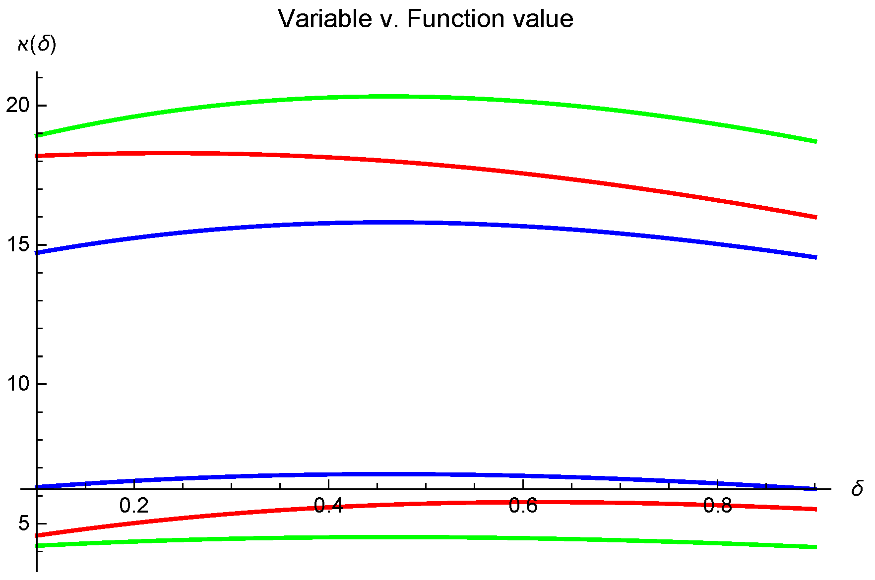
Example 2. 

Let $\Xi \left(\mathfrak{y}\right)=\left[-4{\mathfrak{y}}^2+4,8{\mathfrak{y}}^2+5\right],\gamma \left(\varpi \right)=1,\mathfrak{y}=\left[0,1\right],\delta =1$, then Theorem 8 implies that

$$\begin{array}{c}\hfill \left[6,14\right]{⪯}_{\mathcal{CR}}\left[5.33,15.33\right]{⪯}_{\mathcal{CR}}\left[4,18\right].\end{array}$$

For the purpose of visually representing Theorem 8, we will use the same assumptions as used in the numerical calculation. However, in this case, we will set $\delta \in (0,1)$. Theorem 8 is satisfied.

Figure 2 presents visual analysis of Theorem 8.

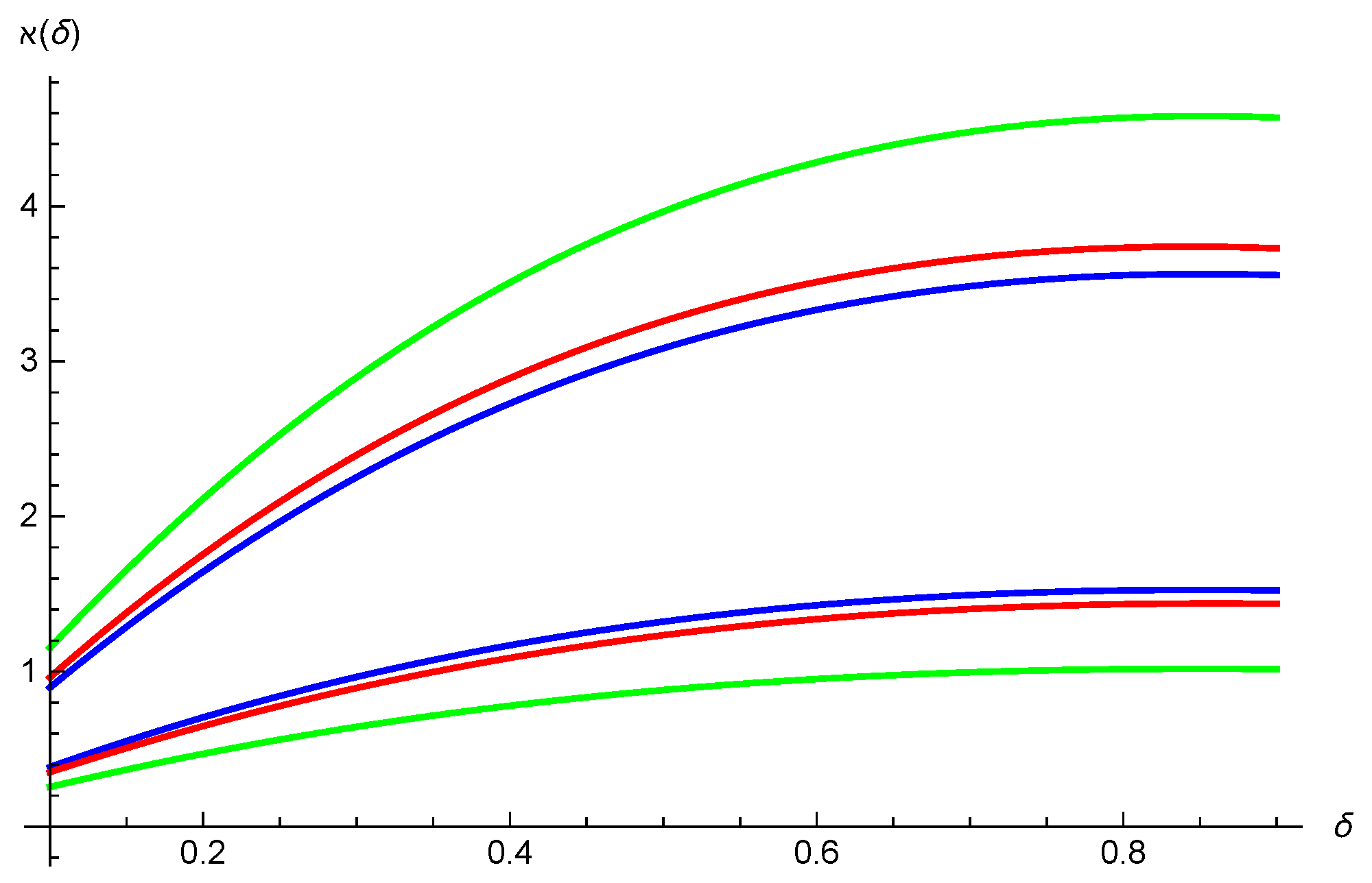
Example 3. 

Let $\Xi \left(\mathfrak{y}\right)=\left[-4{\mathfrak{y}}^2+4,8{\mathfrak{y}}^2+5\right],\wp \left(\mathfrak{y}\right)=\left[-5{\mathfrak{y}}^3+5,9{\mathfrak{y}}^3+6\right]\gamma \left(\varpi \right)=1,\mathfrak{y}=\left[0,1\right], \delta =1$, then Theorem 9 implies that

$$\begin{array}{c}\hfill \left[30,138.5\right]{⪯}_{\mathcal{CR}}\left[13.3,186\right].\end{array}$$

For the purpose of visually representing Theorem 9, we will use the same assumptions as used in the numerical calculation. However, in this case, we will set $\delta \in (0,1)$, then Theorem 9 is satisfied.

Figure 3 presents visual analysis of Theorem 9.

Example 4. 

Let $\Xi \left(\mathfrak{y}\right)=\left[-4{\mathfrak{y}}^2+4,8{\mathfrak{y}}^2+5\right],\wp \left(\mathfrak{y}\right)=\left[-5{\mathfrak{y}}^3+5,9{\mathfrak{y}}^3+6\right]\gamma \left(\varpi \right)=1,\mathfrak{y}=\left[0,1\right],\delta =1$; then, Theorem 10 implies that

$$\begin{array}{c}\hfill \left[52.44,199.48\right]{⪯}_{\mathcal{CR}}\left[36.6,308\right].\end{array}$$

For the purpose of visually representing Theorem 10, we will use the same assumptions as used in the numerical calculation. However, in this case, we will set $\delta \in (0,1)$, then Theorem 10 is satisfied.

Figure 4 presents visual analysis of Theorem 10.

Example 5. 

Let $\Xi \left(\mathfrak{y}\right)=\left[-4{\mathfrak{y}}^2+4,8{\mathfrak{y}}^2+5\right],\wp \left(\mathfrak{y}\right)=\left[-5{\mathfrak{y}}^3+5,9{\mathfrak{y}}^3+6\right]\gamma \left(\varpi \right)=1,\mathfrak{y}=\left[0,1\right],\delta =1$, $P\left(\mathfrak{x}\right)=\mathfrak{x}$ for $\mathfrak{x}\in [0,\frac{1}{2}]$ and $P\left(\mathfrak{x}\right)=1-\mathfrak{x}$ for $\mathfrak{x}\in [\frac{1}{2},1]$, then Theorem 11 implies that

$$\begin{array}{c}\hfill \left[1.5,3.5\right]{⪯}_{\mathcal{CR}}\left[1.4,3.66\right]{⪯}_{\mathcal{CR}}\left[1,4.5\right].\end{array}$$

For the purpose of visually representing Theorem 11, we will use the same assumptions as used in the numerical calculation. However, in this case, we will set $\delta \in (0,1)$, then Theorem 11 is satisfied.

Figure 5 presents visual analysis of Theorem 11.

5. Applications to Special Means

For positive real numbers ${\aleph }^{‡},{\aleph }_{†}$ and ${\aleph }^{‡}\ne {\aleph }_{†}$, the following means are well known:

• The arithmetic mean

  $$\begin{array}{c}\hfill A({\aleph }^{‡},{\aleph }_{†})=\frac{{\aleph }^{‡}+{\aleph }_{†}}{2}.\end{array}$$
• The generalized log mean

  $$\begin{array}{c}\hfill L_p({\aleph }^{‡},{\aleph }_{†})={\left(\frac{{{\aleph }_{†}}^{p+1}-{{\aleph }^{‡}}^{p+1}}{(p+1)({\aleph }_{†}-{\aleph }^{‡})}\right)}^{\frac{1}{p}},p\in \mathbb{R}\setminus \{-1,0\}\end{array}$$

Proposition 3. 

Let ${\aleph }^{‡},{\aleph }_{†}\in \mathbb{R}$ and ${\aleph }^{‡}<{\aleph }_{†}$; then, the following inequality holds:

$$\begin{array}{cc}\hfill \left[-4A^2({\aleph }^{‡},{\aleph }_{†})+4,8A^2({\aleph }^{‡},{\aleph }_{†})+5\right]& {⪯}_{cr}\left[-4L_2^2({\aleph }^{‡},{\aleph }_{†})+4,8L_2^2({\aleph }^{‡},{\aleph }_{†})+5\right]\hfill \\ \hfill & {⪯}_{cr}\left[-4A\left({{\aleph }^{‡}}^2,{{\aleph }_{†}}^2\right)+4,8A\left({{\aleph }^{‡}}^2,{{\aleph }_{†}}^2\right)+5\right].\hfill \end{array}$$

Proof. 

By taking $\gamma \left(\omega \right)=1,\delta =1$ and $\Xi \left(\mathfrak{y}\right)=[-4{\mathfrak{y}}^2+4,8{\mathfrak{y}}^2+5]$ in Theorem 8, we have

$$\begin{array}{c}\hfill \Xi \left(\frac{{\aleph }^{‡}+{\aleph }_{†}}{2}\right){⪯}_{cr}\frac{1}{{\aleph }_{†}-{\aleph }^{‡}}\underset{{\aleph }^{‡}}{\overset{{\aleph }_{†}}{\int }}\Xi \left(\mathfrak{y}\right)d\mathfrak{y}{⪯}_{cr}\frac{\Xi \left({\aleph }^{‡}\right)+\Xi \left({\aleph }_{†}\right)}{2},\end{array}$$

then

$$\begin{array}{cc}\hfill \left[-4{\left(\frac{{\aleph }^{‡}+{\aleph }_{†}}{2}\right)}^2+4,8{\left(\frac{{\aleph }^{‡}+{\aleph }_{†}}{2}\right)}^2+5\right]& {⪯}_{cr}\left[-4\left(\frac{{\left({\aleph }_{†}\right)}^3-{\left({\aleph }^{‡}\right)}^3}{3\left({\aleph }_{†}-{\aleph }^{‡}\right)}\right)+4,8\left(\frac{{\left({\aleph }_{†}\right)}^3-{\left({\aleph }^{‡}\right)}^3}{3\left({\aleph }_{†}-{\aleph }^{‡}\right)}\right)+5\right]\hfill \\ \hfill & {⪯}_{cr}\left[-4\left(\frac{{\left({\aleph }^{‡}\right)}^2+{\left({\aleph }_{†}\right)}^2}{2}\right)+4,8\left(\frac{{\left({\aleph }^{‡}\right)}^2+{\left({\aleph }_{†}\right)}^2}{2}\right)+5\right].\hfill \end{array}$$

This implies that

$$\begin{array}{cc}\hfill \left[-4A^2({\aleph }^{‡},{\aleph }_{†})+4,8A^2({\aleph }^{‡},{\aleph }_{†})+5\right]& {⪯}_{cr}\left[-4L_2^2({\aleph }^{‡},{\aleph }_{†})+4,8L_2^2({\aleph }^{‡},{\aleph }_{†})+5\right]\hfill \\ \hfill & {⪯}_{cr}\left[-4A\left({{\aleph }^{‡}}^2,{{\aleph }_{†}}^2\right)+4,8A\left({{\aleph }^{‡}}^2,{{\aleph }_{†}}^2\right)+5\right].\hfill \end{array}$$

□

6. Conclusions

Over the years, classical integrals inequalities have been generalized by different innovative and novel techniques, such as by employing fractional calculus, quantum calculus, and fuzzy concepts. A significant amount of fractional variants of Hermite–Hadamard-type inequalities are present. For the sake of the unification of trapezium-type inclusions, we organized the current investigation. In the current study, we introduced a new class of interval-valued convexity named $\mathcal{CR}$-$\gamma$, involving a non-negative mapping $\gamma$ and $\mathcal{CR}$ ordering relation, which is the total order relation. We discussed some fundamental integral inequalities as applications. Initially, we computed new generalizations of Jensen’s type containments and their consequences. By making use of this generic class and fractional concepts, we proposed new fractional analogs of Hermite–Hadamard inequality; its weighted form is associated with a symmetric function at about the mid-point and Pachpatte’s type inclusions for the product of two I.V $\mathcal{CR}$-$\gamma$ convex functions. We also verified our primary findings via numeric examples and graphical illustrations. In future, we will study this class from the perspective of the fuzzy domain and, hopefully, this class will play a vital role in the theory of inequalities and other related problems in optimization.

References

- Mitrinović, D.S.; Lacković, I.B. Hermite and convexity. Aequationes Math. 1985, 28, 229–232. [Google Scholar] [CrossRef]
- Dragomir, S.S. Inequalities of Hermite-Hadamard type for h-convex functions on linear spaces. Proyecciones 2015, 34, 323–341. [Google Scholar] [CrossRef]
- Kirmaci, U.S.; Bakula, M.K.; Özdemir, M.E.; Pečarić, J. Hadamard-type inequalities for s-convex functions. Appl. Math. Comput. 2007, 193, 26–35. [Google Scholar] [CrossRef]
- İşcan, İ. A new generalization of some integral inequalities for (α-m)-convex functions. Math. Sci. 2013, 7, 1–8. [Google Scholar] [CrossRef] [Green Version]
- Iscan, I. Hermite-Hadamard type inequalities for p-convex functions. Int. J. Anal. Appl. 2016, 11, 137–145. [Google Scholar]
- Awan, M.U.; Noor, M.A.; Safdar, F.; Islam, A.; Mihai, M.V.; Noor, K.I. Hermite-Hadamard type inequalities with applications. Miskolc Math. Notes 2020, 21, 593–614. [Google Scholar] [CrossRef]
- Awan, M.U.; Talib, S.; Noor, M.A.; Noor, K.I. On γ-preinvex functions. Filomat 2020, 34, 4137–4159. [Google Scholar] [CrossRef]
- Moore, R.E. Interval Analysis; Prentice-Hall: Englewood Cliff, NJ, USA, 1966. [Google Scholar]
- Moore, R.E.; Kearfott, R.B.; Cloud, M.J. Introduction to Interval Analysis; Society for Industrial and Applied Mathematics: Philadelphia, PA, USA, 2009. [Google Scholar]
- Zhao, D.; An, T.; Ye, G.; Liu, W. New Jensen and Hermite-Hadamard type inequalities for h-convex interval-valued functions. J. Inequalities Appl. 2018, 2018, 302. [Google Scholar] [CrossRef] [Green Version]
- An, Y.; Ye, G.; Zhao, D.; Liu, W. Hermite-Hadamard type inequalities for interval (h1, h2)-convex functions. Mathematics 2019, 7, 436. [Google Scholar] [CrossRef] [Green Version]
- Zhao, D.; Ali, M.A.; Murtaza, G.; Zhang, Z. On the Hermite-Hadamard inequalities for interval-valued coordinated convex functions. Adv. Differ. Equ. 2020, 2020, 570. [Google Scholar] [CrossRef]
- Srivastava, H.M.; Sahoo, S.K.; Mohammed, P.O.; Baleanu, D.; Kodamasingh, B. Hermite-Hadamard type inequalities for interval-valued preinvex functions via fractional integral operators. Int. J. Comput. Intel. Syst. 2022, 15, 8. [Google Scholar] [CrossRef]
- Bin-Mohsin, B.; Rafique, S.; Cesarano, C.; Javed, M.Z.; Awan, M.U.; Kashuri, A.; Noor, M.A. Some General Fractional Integral Inequalities Involving LR-Bi-Convex Fuzzy Interval-Valued Functions. Fractal Fract. 2022, 6, 565. [Google Scholar] [CrossRef]
- Mohsin, B.B.; Awan, M.U.; Javed, M.Z.; Budak, H.; Khan, A.G.; Noor, M.A. Inclusions Involving Interval-Valued Harmonically Co-Ordinated Convex Functions and Raina’s Fractional Double Integrals. J. Math. 2022, 2022, 5815993. [Google Scholar] [CrossRef]
- Bhunia, A.K.; Samanta, S.S. A study of interval metric and its application in multi-objective optimization with interval objectives. Comput. Ind. Eng. 2014, 74, 169–178. [Google Scholar] [CrossRef]
- Shi, F.; Ye, G.; Liu, W.; Zhao, D. cr-h-convexity and some inequalities for -h-convex function. Filomat 2022. [Google Scholar]
- Rahman, M.S.; Shaikh, A.A.; Bhunia, A.K. Necessary and sufficient optimality conditions for non-linear unconstrained and constrained optimization problem with interval valued objective function. Comput. Ind. Eng. 2020, 147, 106634. [Google Scholar] [CrossRef]
- Liu, W.; Shi, F.; Ye, G.; Zhao, D. The Properties of Harmonically cr-h-Convex Function and Its Applications. Mathematics 2022, 10, 2089. [Google Scholar] [CrossRef]
- Sahoo, S.K.; Latif, M.A.; Alsalami, O.M.; Treanţǎ, S.; Sudsutad, W.; Kongson, J. Hermite-Hadamard, Fejér and Pachpatte-Type Integral Inequalities for Center-Radius Order Interval-Valued Preinvex Functions. Fractal Fract. 2022, 6, 506. [Google Scholar] [CrossRef]
- Anastassiou, G.A. Advanced Inequalities; World Scientific: Singapore, 2011; Volume 11. [Google Scholar]
- Kilbas, A.A.; Srivastava, H.M.; Trujillo, J.J. Theory and Applications of Fractional Differential Equations; Elsevier: Amsterdam, The Netherlands, 2006; Volume 204. [Google Scholar]
- Miller, K.S.; Ross, B. An Introduction to the Fractional Calculus and Fractional Differential Equations; Wiley: Hoboken, NJ, USA, 1993. [Google Scholar]
- Lupulescu, V. Fractional calculus for interval-valued functions. Fuzzy Sets Syst. 2015, 265, 63–85. [Google Scholar] [CrossRef]
- Budak, H.; Tunc, T.; Sarikaya, M. Fractional Hermite-Hadamard-type inequalities for interval-valued functions. Proc. Am. Math. Soc. 2020, 148, 705–718. [Google Scholar] [CrossRef] [Green Version]
- İscan, İ.; Wu, S. Hermite-Hadamard type inequalities for harmonically convex functions via fractional integrals. Appl. Math. Comput. 2014, 238, 237–244. [Google Scholar]
- İscan, I. Generalization of different type integral inequalities for s-convex functions via fractional integrals. Appl. Anal. 2014, 93, 1846–1862. [Google Scholar] [CrossRef] [Green Version]
- Noor, M.A.; Cristescu, G.; Awan, M.U. Generalized Fractional Hermite-Hadamard Inequalities for Twice Differentiable s-Convex Functions. Filomat 2015, 29, 807–815. [Google Scholar] [CrossRef]
- Wang, J.; Li, X.; Fecbrevekan, M.; Zhou, Y. Hermite-Hadamard-type inequalities for Riemann-Liouville fractional integrals via two kinds of convexity. Appl. Anal. 2013, 92, 2241–2253. [Google Scholar] [CrossRef]
- Fardi, M.; Zaky, M.A.; Hendy, A.S. Nonuniform difference schemes for multi-term and distributed-order fractional parabolic equations with fractional Laplacian. Math. Comput. Simul. 2023, 206, 614–635. [Google Scholar] [CrossRef]
- Fardi, M.; Al-Omari, S.K.Q.; Araci, S. A pseudo-spectral method based on reproducing kernel for solving the time-fractional diffusion-wave equation. Adv. Contin. Discret. Model. 2022, 2022, 54. [Google Scholar] [CrossRef]
- Mohammadi, S.; Ghasemi, M.; Fardi, M. A fast Fourier spectral exponential time-differencing method for solving the time-fractional mobile-immobile advection-dispersion equation. Comput. Appl. Math. 2022, 41, 264. [Google Scholar] [CrossRef]
- Fardi, M.; Khan, Y. A fast difference scheme on a graded mesh for time-fractional and space distributed-order diffusion equation with nonsmooth data. Int. J. Mod. Phys. 2022, 36, 2250076. [Google Scholar] [CrossRef]
- Fardi, M.; Ghasemi, M. A numerical solution strategy based on error analysis for time-fractional mobile/immobile transport model. Soft Comput. 2021, 25, 11307–11331. [Google Scholar] [CrossRef]