Article

Computational Techniques for Solving Mixed (1 + 1) Dimensional Integral Equations with Strongly Symmetric Singular Kernel

by
Sharifah E. Alhazmi
1,
Amr M. S. Mahdy
2,3,*,
Mohamed A. Abdou
4 and
Doaa Sh. Mohamed
2
1
Mathematics Department, Al-Qunfudah University College, Umm Al-Qura University, Al-Qunfudhah 21955, Saudi Arabia
2
Department of Mathematics, Faculty of Science, Zagazig University, Zagazig 44519, Egypt
3
Department of Mathematics & Statistics, College of Science, Taif University, Taif 21944, Saudi Arabia
4
Department of Mathematics, Faculty of Education, Alexandria University, Alexandria 21526, Egypt
*
Author to whom correspondence should be addressed.
Symmetry 2023, 15(6), 1284; https://doi.org/10.3390/sym15061284
Submission received: 3 May 2023 / Revised: 30 May 2023 / Accepted: 5 June 2023 / Published: 19 June 2023

Abstract

:
This paper describes an effective strategy based on Lerch polynomial method for solving mixed integral equations (MIE) in position and time with a strongly symmetric singular kernel in the space L 2 ( 1 , 1 ) × C [ 0 , T ] , ( T < 1 ) . The Quadratic numerical method (QNM) was applied to obtain a system of Fredholm integral equations (SFIE), then the Lerch polynomials method (LPM) was applied to transform SFIE into a system of linear algebraic equations (SLAE). The existence and uniqueness of the integral equation’s solution are discussed using Banach’s fixed point theory. Also, the convergence and stability of the solution and the stability of the error are discussed. Several examples are given to illustrate the applicability of the presented method. The Maple program obtains all the results. A numerical simulation is carried out to determine the efficacy of the methodology, and the results are given in symmetrical forms. From the numerical results, it is noted that there is a symmetry utterly identical to the kernel used when replacing each x with y.

1. Introduction

Singular integral equations (SIE) played a fundamental role in several fields, such as mathematical physics, engineering, elasticity, fluid mechanics, and chemical reactions. SIE of the the first kind can be solved analytically using the following techniques: singular integral equation technique (Cauchy technique), Potential theory technique, Fourier transformation technique, and Krein’s technique. Analytical techniques always fail to find solutions for single-core integral equations of the second kind. The same applies to mixed integral equations. Therefore, researchers find approximate solutions using semi-analytical methods or explicitly numerical techniques. Jafarian et al. [1] used the Bernstein polynomials technique for solving Abel integral equations. A unique approach to solving second-kind Volterra integral equations with discontinuous kernels is presented by Noeiaghdam and Micula in their paper [2]. Nadir [3] applied a quadratic technique for solving SIE of the first kind. Khairullina and Makletsov [4] studied the solution of SIE by the Wavelet collocation method. Gabdulkhaev and Tikhonov [5] applied general projection and projection-iteration techniques for solving SIE with the Cauchy kernel in the real line. Jinyuan [6] used the collocation method to obtain the solution of SIE with the Hilbert kernel. Ahmadi et al. [7] studied the solution of SIE with Cauchy kernel by Chebyshev polynomials. Nadir [8] used spline approximation to get the solution of SIE with a logarithmic kernel. Mahdy and Mohamed [9] studied the solution of SIE by Lucas polynomial method. Seifi [10] presented a Bessel polynomial for solving SIE. Seifi et al. [11] studied the solution of SIE by Bernstein polynomial. Also, different methods exist for solving MIE in position and time with singular and weakly singular kernels. Abdou et al. [12] used a quadratic numerical method for solving MIE with a singular kernel. Abdou and Abd Al-Kader [13] studied the solution of MIE with Potential Kernel by Legendre and Jacobi polynomials. Abdou and Youssef [14] used analytic and numerical methods for solving three MIE with singular kernels. Chokri [15] studied the solution of MIE with a weakly singular kernel by Legendre Polynomials. Jan [16] used the Toeplitz matrix technique to solve MIE with single kernels. While in [17], Jan applied Hermite and Laguerre polynomials for solving nonlinear MIE. Al Hazmi [18] used a projection-iterated method to obtain the solution of MIE. Matoog [19] used the Toeplitz matrix method to solve SIE. In [20], Maleknejad et al. presented a numerical method passing on Jacobi polynomials and the Newton algorithm to approximate the solutions of nonlinear fractional Fredholm and Volterra integral equations in two dimensions. In [21], Liaqat et al. presented Shehu transform and the Adomian decomposition technique in a novel algorithm form to establish approximate and exact solutions to quantum mechanics models. In [22], Attia et al. used to solve a number of major fractional differential equations numerically. Azeem et al. conducted research on the fractional order cancer model with stem cells and treatment utilizing the fractional derivative for their findings, which were published in [23]. Few papers applied LPM. Mohamed [24] presented the solution of SIE with Cauchy kernel using LPM. Cayan and Sezer [25,26,27] used the Lerch matrix collocation algorithm for solving 2D and 3D Volterra integral equations, in [25]. While in [26], they studied the solution of the convection-diffusion problem using LPM. Finally, in [27], they presented the approximate solution of the Neumann Problem by LPM.
This paper is considered one of the rare papers in mathematical physics, as it links the study of the problem in time and space. This gives the authors a more in-depth view of how to study and solve the problem using multiple numerical methods.
Consider the MIE of the third kind with strongly symmetric singular kernel:
μ ( x , t ) Φ ( x , t ) = f ( x , t ) + β 0 t 1 1 F ( t , τ ) 1 ( x y ) 2 Φ ( y , τ ) d y d τ ,
under the boundary conditions:
Φ ( 1 , t ) = Φ ( 1 , t ) = 0 , t [ 0 , T ] , T < 1 ,
where f ( x , t ) and F ( t , τ ) are known functions, μ ( x , t ) is a continuous function defines the kind of MIE, μ ( x , t ) = 0 , for the first kind, μ ( x , t ) = μ = constant 0 , of the second kind, and μ ( x , t ) is variable for the third kind, β is a constant and Φ ( x , t ) is the unknown function.
The paper aims is obtaining the solution to MIE with a strong symmetry kernel in position and continuous kernel in time in the space L 2 ( 1 , 1 ) × C [ 0 , T ] . For this, we use the quadratic method to transform the mixed integral equation, in time and position to SFIEs in position. Then, using Lerch polynomial method, we transform SFIEs into SLAEs. The LPM provides a numerical solution in a rapid convergent power series with an elegantly computable series of terms. The LMC method has proven to be very effective and results in considerable computation time and accuracy savings. The method’s main advantage is that it can remove the singularity and transform the SIE into SLAE, which is easy to solve numerically. Also, no author has used the numerical approach in this publication to solve this application.
In the remaining sections of the article are laid out based on the following: In Section 2, MIE’s existence and unique solutions are discussed. Section 3 is devoted to studying the convergence and stability of the solution. Section 4 applies the QNM to transform the MIE into an SFIE. The existence of a unique solution to the SFIE is discussed in Section 5. In Section 6, LPM is presented to transform SFIE into SLAE. The stability of the error is presented in Section 7. In Section 8, some numerical results are given to illustrate the effectiveness of the proposed algorithms. Conclusion of the paper and Analysis of the results presented in Section 9.

2. Existence and Unique Solution of MIE

Banach’s fixed point theory discusses the existence and uniqueness solution of the MIE (1). For this, we write (1) in the integral operator form:
T ¯ Φ ( x , t ) = f ( x , t ) μ ( x , t ) + β μ ( x , t ) T Φ ( x , t ) , ( μ ( x , t ) 0 , β 0 ) ,
T Φ ( x , t ) = 0 t 1 1 F ( t , τ ) P ( x y ) Φ ( y , τ ) d y d τ , P ( x y ) = 1 ( x y ) 2 .
Then, suppose the next conditions
(I) 
the kernel of position satisfies
{ 1 1 1 1 { P 2 ( x y ) d x d y } 1 2 p * ,
p * is constant.
(II) 
The kernel of time F ( t , τ ) C [ 0 , T ] satisfies F ( t , τ ) M , M is a constant t [ 0 , T ] ,   T < 1 .
(III) 
The function f ( x , t ) , with its partial derivatives with respect to x and t are continuous in L 2 ( 1 , 1 ) × C [ 0 , T ] , T < 1 and for constant f * its norm is
f ( x , t ) L 2 ( 1 , 1 ) × C [ 0 , T ] = max 0 = t T < 1 0 t { 1 1 f 2 ( x , τ ) d x } 1 2 d τ = f * ,
μ ( x , t ) μ * .
(IV) 
The function Φ ( x , t ) , behaves in L 2 ( 1 , 1 ) × C [ 0 , T ] , as the free function f ( x , t ) and its norm is defined as Φ ( x , t ) = Φ * .
Theorem 1. 
The MIE (1) has an existence and unique solution, under the condition
β M T p * < μ * .
To prove the existence and uniqueness of the solution for the MIE (1) we must prove the next two lemmas:
Lemma 1. 
According to the conditions (I)–(IV), and in the space L 2 (−1, 1) × C[0, T], T < 1, the operator T ¯ maps the space into itself.
Proof. 
Depending with the conditions (II) and (III), after implementation Hölder inequality, the IE (3) yields
T ¯ Φ ( x , t ) f * μ * + M β μ * max 0 t T [ 1 1 1 1 P ( x y ) 2 d x d y ] max 0 t T 0 t { 1 1 Φ ( y , τ ) 2 d y } 1 2 d τ .
From conditions (I), (II) and (IV), we have
T ¯ Φ ( x , t ) f * μ * + α Ψ ( x , t ) , ( α = β μ * M p * T ) .
The inequality (6) tells us which the operator T ¯ maps the ball S ϱ into itself, where
ϱ = f * [ μ * β M p * T ] , ( ϱ > 0 ) .
Consequently, we get α < 1 . Additionally, the inequality (6) includes the limitation of the integral operator T , where
T Φ ( x , t ) = T Φ ( x , t ) α Φ ( x , t ) .
Lemma 2. 
Under the conditions (I), (II) and (IV), the integral operator T ¯ is a contraction in the space L 2 (−1, 1) × C[0, T].
Proof. 
Assume the two different functions { Φ 1 ( x , t ) , Φ 2 ( x , t ) } L 2 ( 1 , 1 ) × C [ 0 , T ] , then we have
T ¯ Φ 1 ( x , t ) T ¯ Φ 2 ( x , t ) β μ 0 t 1 1 F ( t , τ ) P ( x y ) Φ 1 ( y , τ ) Φ 2 ( y , τ ) d y d τ .
After using conditions (II) and (IV), the above inequality develop into
T ¯ Φ 1 ( x , t ) T ¯ Φ 2 ( x , t ) β μ * M P ( x y ) 0 t 1 1 Φ 1 ( y , τ ) Φ 2 ( y , τ ) d y d τ .
Applying Hölder inequality, then using condition (I), we obtain
T ¯ Φ 1 ( x , t ) T ¯ Φ 2 ( x , t ) α Φ 1 ( x , t ) Φ 2 ( x , t ) .
From inequality (9) we decide that: the operator T ¯ is continuous in the space L 2 ( 1 , 1 ) × C [ 0 , T ] , and then it is a contraction operator, according to the case α < 1 . Therefore, with Banach fixed point theory, T ¯ is a unique fixed point that is the unique solution of Equation (3). □

3. Convergence and Stability of Solution

This part dealt with the study of convergence and stability of solutions. For the simple iteration { Φ 0 ( x , t ) , Φ 1 ( x , t ) , , Φ n 1 ( x , t ) , Φ n ( x , t ) , } Φ ( x ; t ) , we can choose two arbitrary functions satisfying the relations
μ ( x , t ) Φ n ( x , t ) = f ( x , t ) + β 0 t 1 1 F ( t , τ ) 1 ( x y ) 2 Φ n 1 ( y , τ ) d y d τ ,
μ ( x , t ) Φ n 1 ( x , t ) = f ( x , t ) + β 0 t 1 1 F ( t , τ ) 1 ( x y ) 2 Φ n 2 ( y , τ ) d y d τ .
Using Equations (10) and (11), we can establish the following integral equation
μ ( x , t ) Ψ n ( x , t ) = β 0 t 1 1 F ( t , τ ) 1 ( x y ) 2 Ψ n 1 ( y , τ ) d y d τ ,
where
Ψ n ( x , t ) = Φ n ( x , t ) Φ n 1 ( x , t ) .
Hence, from the above Equations (12) and (13), we deduce the following
Φ n ( x , t ) = i = 0 n Ψ i ( x , t ) , n = 1 , 2 , ,
and
Ψ 0 ( x , t ) = F ( x , t ) / μ ( x , t ) , μ ( x , t ) 0 ( x , t ) L 2 ( 1 , 1 ) × C [ 0 , T ] .
So, it is clear that if, n , in Equation (14), we have
lim n Φ n ( x , t ) = Φ ( x , t ) = i = 0 Ψ i ( x , t ) .
From Formula (16) tells us that we can construct a new sequence { Ψ i ( x , t ) } i = 0 n and this sequence represents the general solution if n .
Theorem 2. 
Under the conditions (I)–(III) the finite sequence Ψ i ( x , t ) is uniformly convergent and it leads to the unique solution, if n .
Proof. 
Using Cauchy-Schwarz inequality on the domain of integration L 2 ( 1 , 1 ) × C [ 0 , T ] , Equation (12) becomes
μ ( x , t ) ( 0 t ( 1 1 ( Ψ n 2 ( x , t ) ) d x ) d τ ) β ( 0 t F ( t , τ ) d τ ( 1 1 1 1 1 ( x y ) 4 d x d y ) ( 0 t ( 1 1 ( Ψ n 1 2 ( x , t ) ) ) ) d τ ) .
Applying conditions (I) and (II), we have
μ * Ψ n ( x , t ) β p * M T Ψ n 1 ( x , t ) .
The above inequality can adapt to take the form
Ψ n ( x , t ) α Ψ n 1 ( x , t ) , ( α = β M p * T μ * ) .
Using mathematical induction and condition (III), we obtain
Ψ n ( x , t ) α n f * , ( α = β M p * T μ * ) < 1 ) .
Equation (18) shows the convergent sequence { Ψ n ( x , t ) } uniformly, t [ 0 , T ] , x ( 1 , 1 ) . Furthermore, it confirms the convergent solution of the sequence { Φ n ( x , t ) } . Since Ψ n ( x , t ) is uniformly continuous, and
lim n Φ n ( x , t ) = lim n i = 0 n Ψ i ( x , t ) = i = 0 Ψ i ( x , t ) = Φ ( x , t ) ,
hence Φ ( x , t ) is uniformly convergent with an infinite { Φ ( x , t ) } n = 0 series. □

4. Quadratic Numerical Method

In the present section, QNM is applied to transform the MIE of position and time (1) into SFIE in position. For this purpose, we split the interval [ 0 , T ] , 0 τ t T < 1 , as 0 = t 0 < t 1 < < t i < < t N = T , where t = t i , i = 0 , 1 , 2 , , N . Hence Equation (1) can be written in the form:
μ ( x , t i ) Φ ( x , t i ) = f ( x , t i ) + β 0 t i 1 1 F ( t i , τ ) 1 ( x y ) 2 Φ ( y , τ ) d y d τ ,
write Equation (19) in the form
μ ( x , t i ) Φ ( x , t i ) = f ( x , t i ) + β j = 0 i ω j F ( t i , t j ) 1 1 1 ( x y ) 2 Φ ( y , t j ) d y ,
where
ω j = h 2 , j = 0 , h , 0 < j < i , h 2 , j = i . h = T 0 N
Rewrite Equation (20) in the form
μ i ( x ) Φ i ( x ) = f i ( x ) + β j = 0 i ω j F i , j 1 1 1 ( x y ) 2 Φ j ( y ) d y ,
which represents a SFIE, of the third kind
μ i ( x ) = μ ( x , t i ) , Φ i ( x ) = Φ ( x , t i ) , f i ( x ) = f ( x , t i ) , F i , j = F ( t i , t j ) .

5. The Existence of a Unique Solution of the SFIE

To prove the existence of a unique solution of the SFIE (21), let E be the set of all continuous functions in the space L 2 ( 1 , 1 ) × , where Φ ( x ) = { Φ , 0 ( x ) , Φ , 1 ( x ) , , Φ , n ( x ) , } and we can define the norm in the Banach space E by
Φ ( x ) L 2 ( 1 , 1 ) × = max n Φ , n ( x ) .
Under the next conditions
(a)
The kernel of position fulfills Fredholm condition 1 1 1 1 1 ( x y ) 4 d x d y p * ,
(b)
max i ω i F i , j Q , ( Q const) ; max i μ i ( x ) N ,
(c)
max i f i ( x ) L 2 [ 1 , 1 ] × H .
Theorem 3. 
The infinite series i = 0 { χ i } , χ i n = Φ i n ( x ) Φ i n 1 ( x ) convergence uniformly to a continuous function Φ ( x ) .
Proof. 
Constructing a series of solutions in the form is the next step
μ i ( x ) Φ i , n ( x ) = f i ( x ) + β j = 0 i ω j F i , j 1 1 1 ( x y ) 2 Φ j , n 1 ( y ) d y .
Introduce the function χ i such that χ i n = Φ i n ( x ) Φ i n 1 ( x ) . In this case, the integral Equation (22), becomes
μ i ( x ) χ i , n ( x ) = β j = 0 i ω j F i , j 1 1 1 ( x y ) 2 χ j , n 1 ( y ) d y .
Using the norm properties in (23) we following
μ i ( x ) χ i , n ( x ) β j = 0 i ω j F i , j ( 1 1 1 1 1 ( x y ) 4 d x d y ) χ i , n 1 ( x ) .
Using conditions (a)–(b), then with the aid of mathematical induction and condition (c), finally we have
χ i , n 1 ( x ) ρ i n H , ( ρ i n = β p * Q N , i = 0 , 1 , , N ) .
The result of inequality (24) leads to say that the sequence of SFIE (21) is convergence uniformly and the system has a unique solution when n .

6. Lerch Polynomials Method and Singular Integral Equations

In this section LPM applied to obtain the solution of SFIE (21).
Definition 1. 
The formula for the explicit expression of the Lerch polynomials is provided as [28,29,30]:
L m ( ζ , λ ) = = 1 m ! m ! s ( m , ) + λ 1 ζ ,
where L 0 ( ζ , λ ) = 1 is the initial value, λ is a parameter and s ( m , ) is Stirling numbers of the first kind.
Several characteristics of the Stirling numbers [31,32] are as follows:
s ( m + 1 , 0 ) = 0 , s ( m , m ) = 1 , s ( m , 1 ) = ( 1 ) m 1 ( m 1 ) ! , s ( m , m 1 ) = m 2 , m 0 .
From Equation (25), the first six Lerch polynomials are given as follows:
L 0 ( ζ , λ ) = 1 ,
L 1 ( ζ , λ ) = λ ζ ,
L 2 ( ζ , λ ) = λ 2 ζ + λ ( λ + 1 ) 2 ζ 2 ,
L 3 ( ζ , λ ) = λ 3 ζ λ ( λ + 1 ) 2 ζ 2 + λ ( λ + 1 ) ( λ + 2 ) 6 ζ 3 ,
L 4 ( ζ , λ ) = λ 4 ζ + 11 λ ( λ + 1 ) 24 ζ 2 λ ( λ + 1 ) ( λ + 2 ) 4 ζ 3 + λ ( λ + 1 ) ( λ + 2 ) ( λ + 3 ) 24 ζ 4 ,
L 5 ( ζ , λ ) = λ 5 ζ 5 λ ( λ + 1 ) 12 ζ 2 + 7 λ ( λ + 1 ) ( λ + 2 ) 24 ζ 3 λ ( λ + 1 ) ( λ + 2 ) ( λ + 3 ) 12 ζ 4 + λ ( λ + 1 ) ( λ + 2 ) ( λ + 3 ) ( λ + 4 ) 120 ζ 5 .

Lerch Matrix Collocation Method

The truncated Lerch series expression is structured to represent the approximate solution to Equation (21), and it reads as follows:
Φ ( x ) Φ N ( x ) = k = 0 N a k L k ( x , λ ) ,
where a k are the unknown coefficients.
There are three approaches to treating the integral segment with a strong kernel. In this section, we use LPM, as a numerical method. Therefore, it is suitable to use “displacement of singular points”. As for the other two methods, they will be mentioned simply at the end, commenting on the results under the item “conclusion”.
Rewrite the position integral term of Equation (21) in the form:
1 1 Φ j ( y ) ( x y ) 2 d y = 1 1 Φ j ( y ) Φ j ( x ) ( x y ) 2 d y + 1 1 Φ j ( x ) ( x y ) 2 d y = 1 1 Φ j ( y ) Φ j ( x ) ( x y ) 2 d y 2 Φ j ( x ) 1 x 2 .
Substituting from (26), (27) into (21) we obtain
k = 0 N a i , k μ i ( x ) L k ( x , λ ) + β k = 0 N j = 0 i a j , k ω j F i , j 1 1 L k ( x , λ ) L k ( y , λ ) ( x y ) 2 d y = g i ( x ) ,
g i ( x ) = f i ( x ) 2 β k = 0 N j = 0 i a j , k ω j F i , j L j ( x , λ ) 1 x 2 , i = 0 , 1 , , N .
Adapting Equation (28) to take the form
a i , k μ i ( x ) L i ( x , λ ) + β { a 0 , k ω 0 F i , 0 1 1 L 0 ( x , λ ) L 0 ( y , λ ) ( x y ) 2 d y + a 1 , k ω 1 F i , 1 1 1 L 1 ( x , λ ) L 1 ( y , λ ) ( x y ) 2 d y
+ a 2 , k ω 2 F i , 2 1 1 L 2 ( x , λ ) L 2 ( y , λ ) ( x y ) 2 d y } + β j = 3 i a j , k ω j F i , j 1 1 L k ( x , λ ) L k ( y , λ ) ( x y ) 2 d y = g i ( x ) , i , k = 0 , 1 , , N .
Using the values of L 0 ( x , λ ) , L 1 ( x , λ ) , L 2 ( x , λ ) in the integral terms of (29), we follow
1 1 L 0 ( x , λ ) L 0 ( y , λ ) ( x y ) 2 d y = 0 , 1 1 L 1 ( x , λ ) L 1 ( y , λ ) ( x y ) 2 d y = λ ln 1 x 1 + x ,
1 1 L 2 ( x , λ ) L 2 ( y , λ ) ( x y ) 2 d y = λ 2 ln 1 x 1 + x + 2 λ ( λ + 1 ) [ x ln 1 x 1 + x 1 ] .
Introducing Equation (30) in Equation (29), we have
a i , k μ i ( x ) L i ( x , λ ) + β λ { a 1 , k ω 1 F i , 1 ln 1 x 1 + x + a 2 , k ω 2 F i , 2 [ 1 2 ln 1 + x 1 x + 2 ( λ + 1 ) ( x ln 1 + x 1 x 1 ) ] }
+ β j = 3 i a j , k ω j F i , j 1 1 L k ( x , λ ) L k ( y , λ ) ( x y ) 2 d y = g i ( x ) , i , k = 0 , 1 , , N .
The formula (31) can adapt in the form
a i , k μ i ( x ) = 1 i ! i ! s ( i , ) x + λ 1 + β j = 3 i a j , k ω j F i , j γ k = Z i ( x ) , i = 0 , 1 , , N ,
where
Z i ( x ) = f i ( x ) 2 β k = 0 N j = 0 i a j , k ω j F i , j L k ( x , λ ) 1 x 2 β λ { a 1 , k ω 1 F i , 1 ln 1 x 1 + x
+ a 2 , k ω 2 F i , 2 [ 1 2 ln 1 + x 1 x + 2 ( λ + 1 ) ( x ln 1 + x 1 x 1 ) } ,
γ k = 1 1 L k ( x , λ ) L k ( y , λ ) ( x y ) 2 d y = = 3 k δ = 0 1 ! k ! s ( k , ) x 1 δ + λ 1 1 1 y δ ( x y ) d y .
Using suitable collocation points x r in the interval (−1,1), such as the collocation points which used in [33], hence Equation (32) reduced to the following SLAE
a i , k μ i ( x r ) = 1 i ! i ! s ( i , ) x r + λ 1 + β j = 3 i a j , k ω j F i , j γ k = Z i ( x r ) , i = 0 , 1 , , N .
Solving the above SLAE we obtain the unknown coefficients, then we obtain the approximate solution from (26).

7. The Stability of the Error

It is known that the error resulting from numerical solutions depends on the error of the method used, then the error resulting from the approximation of the solution, and finally the error of the program used. The error equation is always in the form of the original equation to be solved. In this particular instance, the error produced is represented by the disparity among both the analytical and numerical solutions. If the analytic solution is Φ ( x , t ) and the corresponding numerical solution is approximate to Φ n ( x , t ) . Then the error can be calculated in the form
R n ( x , t ) = [ Φ ( x , t ) Φ n ( x , t ) ] = β μ ( x , t ) 0 t 1 1 F ( t , τ ) ( x y ) 2 [ Φ ( y , τ ) Φ n ( y , τ ) ] d y d τ .
The above equation can adapt in the form
R n ( x , t ) = β μ ( x , t ) 0 t 1 1 F ( t , τ ) ( x y ) 2 R n ( y , τ ) d y d τ .
The reader can prove that: the error of Equation (35), under the condition (I) and (II) is convergence and of order O ( N ( n + 1 ) ) . Also, for the linear system the error integral Equation (35) can take the form
R n ( x ) = β μ i ( x ) j = 0 i ω j F i , j 1 1 R n , j ( y ) ( x y ) 2 d y .
Theorem 4. 
Under the next conditions 1 1 1 1 1 ( x y ) 4 d x d y p * , μ ( x , t ) μ * , F ( t , τ ) M , the error is stable in the space L 2 ( 1 , 1 ) × C [ 0 , T ] .
Proof. 
Since
R n = β μ ( x , t ) 0 t 1 1 F ( t , τ ) [ Φ ( y , τ ) Φ n ( y , τ ) ] ( x y ) 2 .
Using Cauchy-Schwarz inequality on the domain of integration L 2 ( 1 , 1 ) × C [ 0 , T ] , we have
R n β μ * M 1 1 1 1 1 ( x y ) 4 d x d y Φ ( y , τ ) Φ n ( y , τ ) [ max 0 t T 0 t d t ] .
By using the above conditions of Theorem 4, we have
R n β μ * M p * T Φ ( y , τ ) Φ n ( y , τ ) .
The above inequality tells us that if n , then R n 0 .
Theorem 5. 
The representation of the error is unique.
Proof. 
Consider we have two representation of the error such that
R n R m = β μ ( x , t ) 0 t 1 1 F ( t , τ ) [ Φ ( y , τ ) Φ n ( y , τ ) ] ( x y ) 2 β μ ( x , t ) 0 t 1 1 F ( t , τ ) [ Φ ( y , τ ) Φ m ( y , τ ) ] ( x y ) 2 .
Then, we have
R n R m = β μ ( x , t ) 0 t 1 1 F ( t , τ ) [ Φ n ( y , τ ) Φ m ( y , τ ) ] ( x y ) 2 .
i.e.,
R n R m β μ * M p * T Φ n ( y , τ ) Φ m ( y , τ ) .
In the above inequality, if n m , then { ( Φ n ( y , τ ) Φ m ( y , τ ) ) } 0 { ( R n R m ) } 0 .

8. Numerical Computations

In this section implementation examples have been introduced by using QNM and LPM.
Example 1. 
Consider the following MIE of the third kind with strongly symmetric kernel:
μ ( x , t ) Φ ( x , t ) = f ( x , t ) + β 0 t 1 1 t 2 τ 1 ( x y ) 2 Φ ( y , τ ) d y d τ ,
where β = 0.01 , f ( x , t ) is specified by laying Φ ( x , t ) = x 2 t 2 .
  • Case (11), if μ ( x , t ) = 1 , then Equation (37) becomes of the second kind and can be expressed in writing using a format
    Φ ( x , t ) = f ( x , t ) + β 0 t 1 1 t 2 τ 1 ( x y ) 2 Φ ( y , τ ) d y d τ .
  • Case (12), if μ ( x , t ) = ( 0.25 + x 2 ) ( 0.2 + t ) , then Equation (37) becomes of the third kind and written in the form
    ( 0.25 + x 2 ) ( 0.2 + t ) Φ ( x , t ) = f ( x , t ) + β 0 t 1 1 t 2 τ 1 ( x y ) 2 Φ ( y , τ ) d y d τ .
    Now applying QNM and LPM for Equations (38) and (39) when N = 3 , T = { 0 , 0.2 , 0.4 , 0.6 } , λ = 1 .
The approximate solutions in cases (11) and (12) are given in the form:
  • For case (11)  Φ 0 ( x ) = 0 , T = 0 ,
  • Φ 1 ( x ) = 4.939886371 × 10 7 + 0.03999705437 x 2 9.257754842 × 10 13 x 3 , T = 0.2
  • Φ 2 ( x ) = 0.000003947269514 1 × 10 11 x + 0.1599764582 x 2 + 5.793011789 × 10 11 x 3 ,
    T = 0.4
  • Φ 3 ( x ) = 0.0001984052689 + 0.3588153536 x 2 + 2.159505114 × 10 11 x 3 , T = 0.6
  • For case (12)  Φ 0 ( x ) = 0 , T = 0 ,
  • Φ 1 ( x ) = 0.000002450173876 + 1 × 10 11 x + 0.03999146727 e x 2 9.994590610 × 10 12 x 3 ,
    T = 0.2
  • Φ 2 ( x ) = 0.00001303309878 + 0.1599545797 x 2 2.897049790 × 10 14 x 3 , T = 0.4
  • Φ 3 ( x ) = 0.0004891097646 + 0.3582900436 x 2 + 6.441769153 × 10 11 x 3 , T = 0.6 .
The absolute errors in case (11) with different values of x ( 1 , 1 ) are shown in Table 1, Figure 1, Figure 2 and Figure 3 comparison between exact and approximate solution when T = 0.2 approaching in Figure 4, also the absolute errors in case (12) are shown in Table 2, Figure 5, Figure 6 and Figure 7.
In example 1, a relation between the accurate solution and the approximate response is shown in Figure 4 it is clear that the exact solution matches the approximate solution and this indicates the extent and clarity of the method. Also comparison between the absolute errors presented in Figure 1, Figure 2 and Figure 3, Figure 5, Figure 6 and Figure 7 it is clear that if the time increasing, then the error also increasing, this clear also in Table 1 and Table 2.
Example 2. 
Consider the MIE of the third kind:
μ ( x , t ) Φ ( x , t ) = f ( x , t ) + β 0 t 1 1 t 2 τ 1 ( x y ) 2 Φ ( y , τ ) d y d τ ,
where β = 0.01 , f ( x , t ) is specified by laying Φ ( x , t ) = x 2 + t 2 .
  • Case (21) if μ ( x , t ) = 1 , then Equation (40) becomes of the second kind and can be written in the form
    Φ ( x , t ) = f ( x , t ) + β 0 t 1 1 t 2 τ 1 ( x y ) 2 Φ ( y , τ ) d y d τ .
  • Case (22) if μ ( x , t ) = ( 0.25 + x 2 ) e t , then Equation (40) becomes of the third kind and written in the form
    ( 0.25 + x 2 ) e t Φ ( x , t ) = f ( x , t ) + β 0 t 1 1 t 2 τ 1 ( x y ) 2 Φ ( y , τ ) d y d τ .
    Applying QNM and LPM for Equations (41) and (42) when N = 3 , T = { 0 , 0.2 , 0 , 4 , 0.6 } , λ = 1 . The absolute errors in cases (21) and (22) presented in Table 3 and Table 4 and Figure 8, Figure 9, Figure 10, Figure 11, Figure 12 and Figure 13.
In example 2, comparison between the absolute errors presented in Figure 8, Figure 9, Figure 10, Figure 11, Figure 12 and Figure 13 it is clear that if the time increasing, then the error also increasing, this clear also in Table 3 and Table 4.
Example 3. 
Consider the MIE of the third kind:
μ ( x , t ) Φ ( x , t ) = f ( x , t ) + β 0 t 1 1 t 2 τ 2 1 ( x y ) 2 Φ ( y , τ ) d y d τ ,
where β = 0.01 , f ( x , t ) is specified by laying Φ ( x , t ) = x 2 ln ( 1 + t ) .
  • Case (31) if μ ( x , t ) = 1 , then Equation (43) becomes of the second kind and can be written in the form
    Φ ( x , t ) = f ( x , t ) + β 0 t 1 1 t 2 τ 1 ( x y ) 2 Φ ( y , τ ) d y d τ .
  • Case (32) if μ ( x , t ) = ( 0.2 + t ) e x , then Equation (43) becomes of the third kind and written in the form
    ( 0.2 + t ) e x Φ ( x , t ) = f ( x , t ) + β 0 t 1 1 t 2 τ 1 ( x y ) 2 Φ ( y , τ ) d y d τ .
    Applying QNM and LPM for Equations (44) and (45) when N = 3 , T = { 0 , 0.2 , 0 , 4 , 0.6 } , λ = 1 . The absolute errors in cases (31) and (32) presented in Table 5 and Table 6 and Figure 14, Figure 15, Figure 16, Figure 17, Figure 18 and Figure 19.
Similarly as in examples 1 and 2 comparison between the absolute errors of example 3 are presented in Figure 14, Figure 15, Figure 16, Figure 17, Figure 18 and Figure 19 it is clear that if the time increasing, then the error also increasing, this clear also in Table 5 and Table 6.
Example 4. 
Consider the following MIE of the second kind:
Φ ( x , t ) = f ( x , t ) + 0.01 0 t 1 1 t 2 τ 1 ( x y ) 2 Φ ( y , τ ) d y d τ ,
where f ( x , t ) is specified by laying Φ ( x , t ) = x 2 e t .
Similarly as the above examples the absolute errors by using QNM and LPM are presented in Table 7 and Figure 20, Figure 21 and Figure 22:
In example 4, comparison between the absolute errors presented in Figure 20, Figure 21 and Figure 22 it is clear that if the time increasing, then the error also increasing, this clear also in Table 7.

9. Conclusions

In the present work, QNM was implemented to overcome MIE in ( 1 + 1 ) dimensional with a strongly symmetric singular kernel in the space L 2 ( 1 , 1 ) × C [ 0 , T ] , ( T < 1 ) , the MIE is converted to SFIE we can deal with the strong kernel in three techniques:
  • The first technique is removing the singularity which presented in Section 6.
  • The second technique (Cauchy method) is integrating Equation (21) by parts and using the boundary conditions (2), we have
    β j = 0 i ω j F i , j 1 1 d Φ j ( y ) d y ( x y ) d y = μ i ( x ) Φ i ( x ) f i ( x ) = h i ( x ) .
    The above Equation has the solution
    β j = 0 i ω j F i , j d Φ j ( x ) d x = 1 x 2 π 1 1 h i ( y ) 1 y 2 ( x y ) d y , i = 0 , 1 , , N ,
    a solution exists if the next conditions are fulfilled:
    1 1 h i ( y ) 1 y 2 d y = 0 .
  • The third technique (approximate kernel) is to assume the approximate sequence { k n ( x , y ) } be a sequence of kernels that satisfy the condition
    lim n { b b b b k n ( x , y ) k ( x , y ) 2 d x d y } 1 2 = 0 ,
    then there exists a positive integer n 0 , such that
    { b b b b k n ( x , y ) 2 d x d y } 1 2 c < , ( n > n 0 ) .
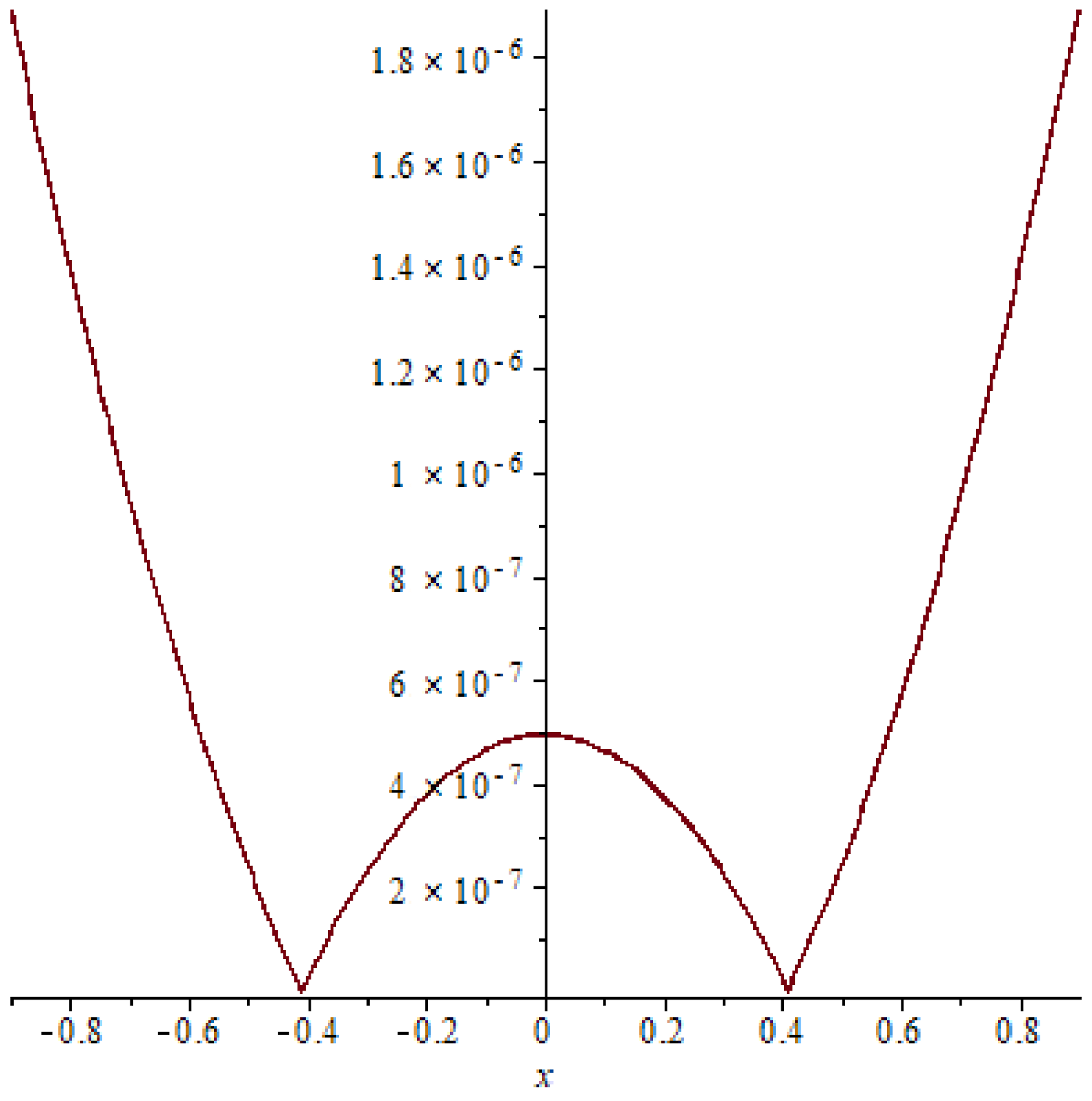
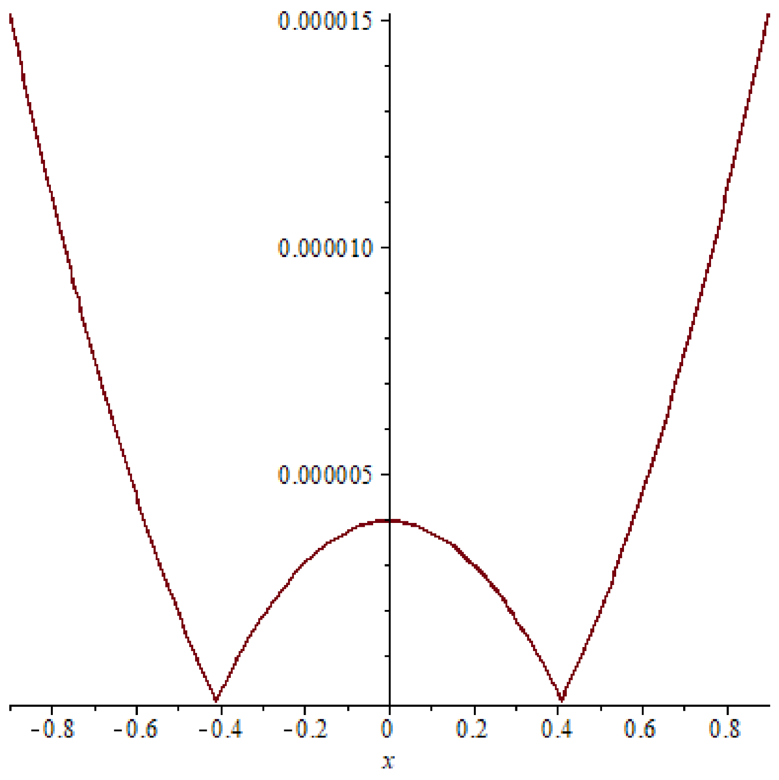
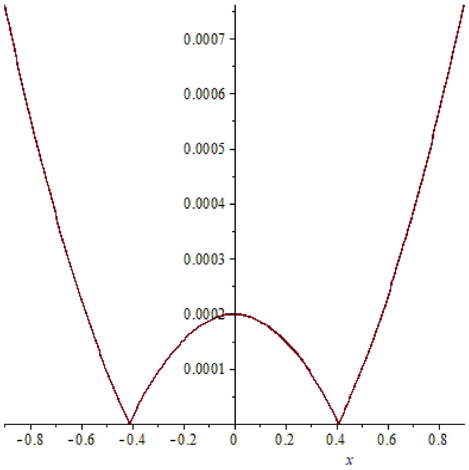
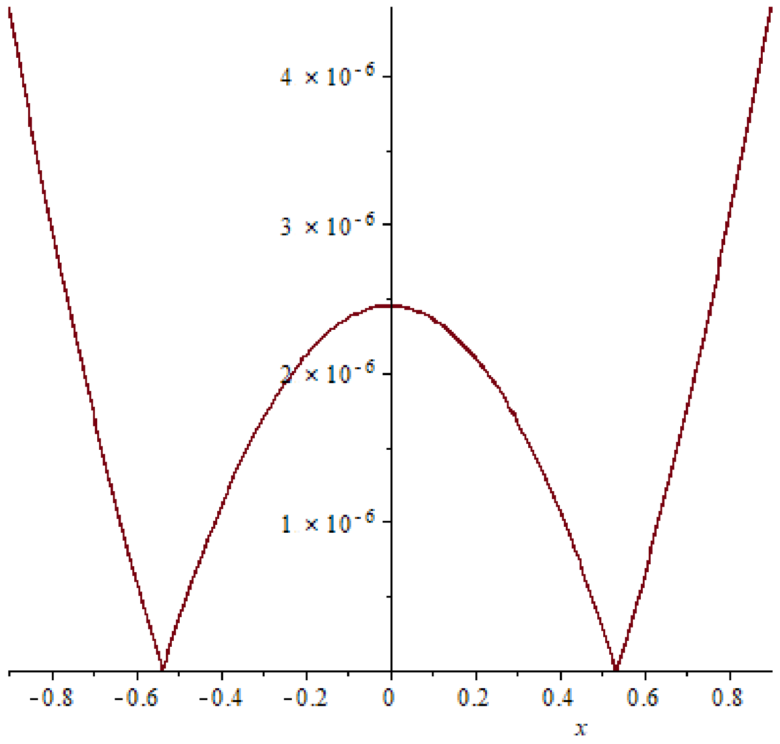
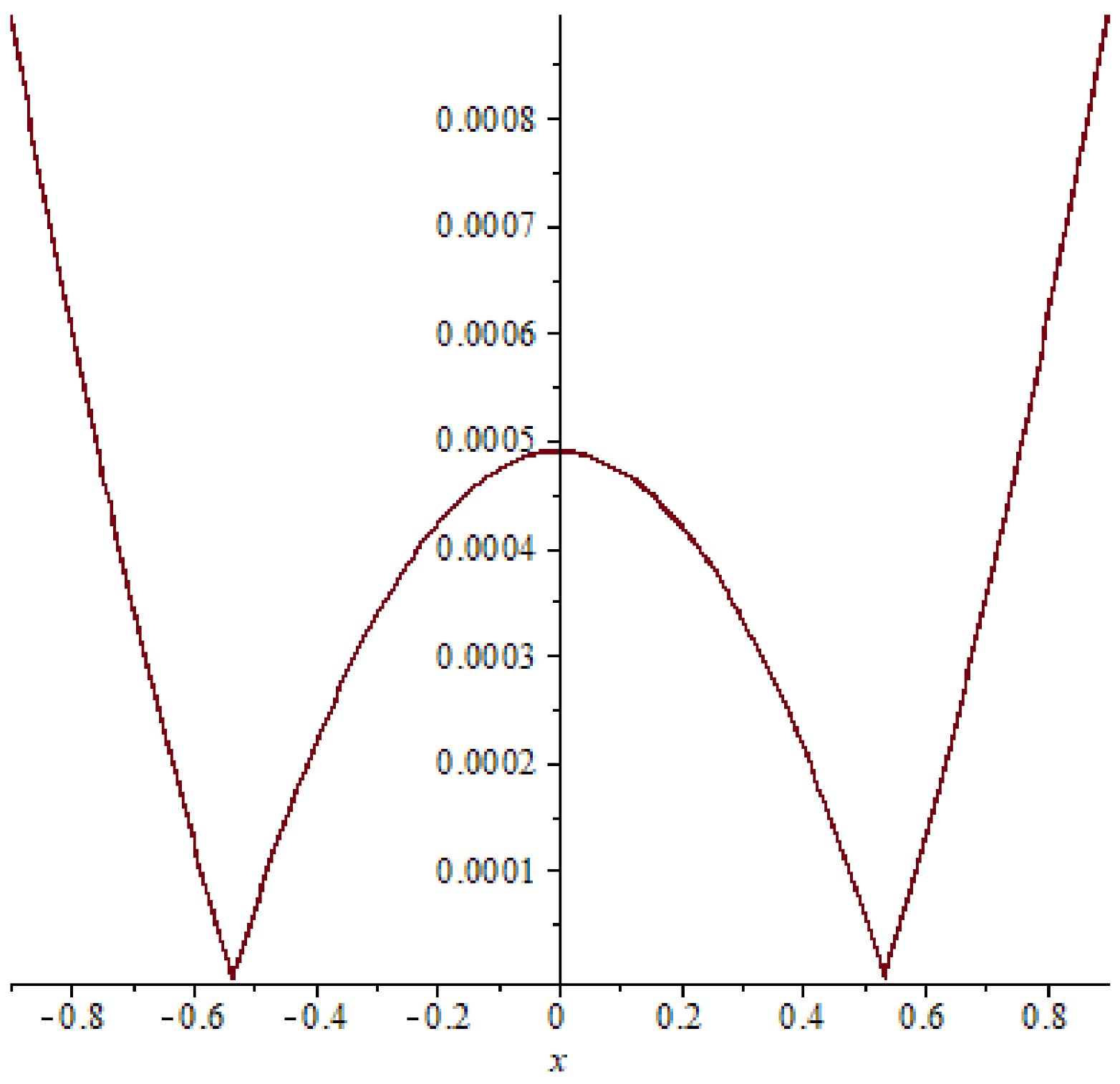
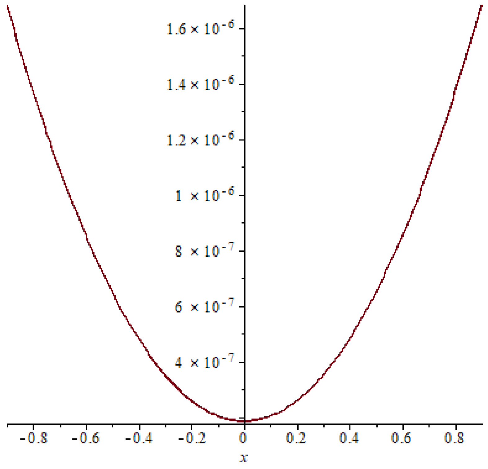
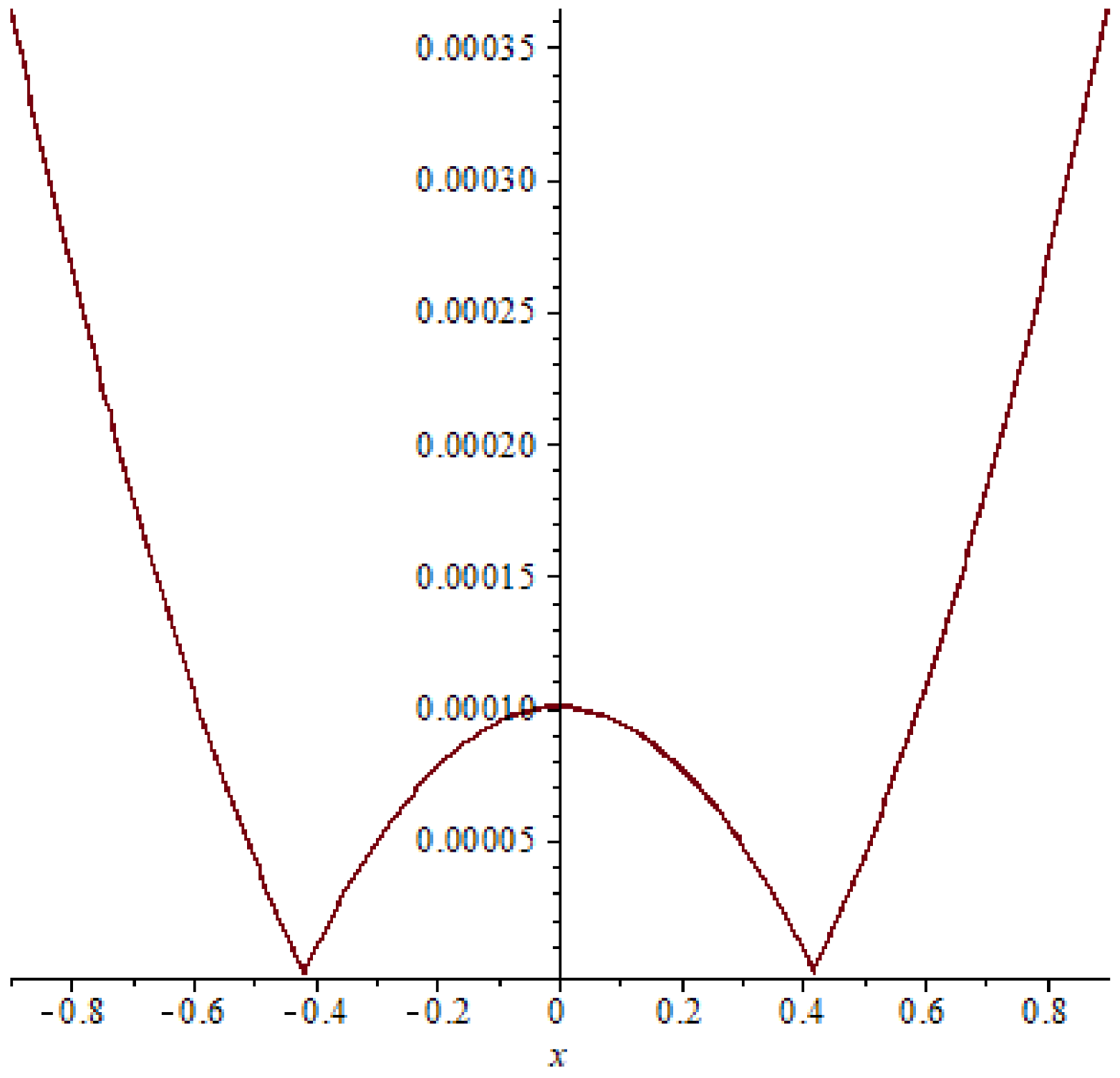
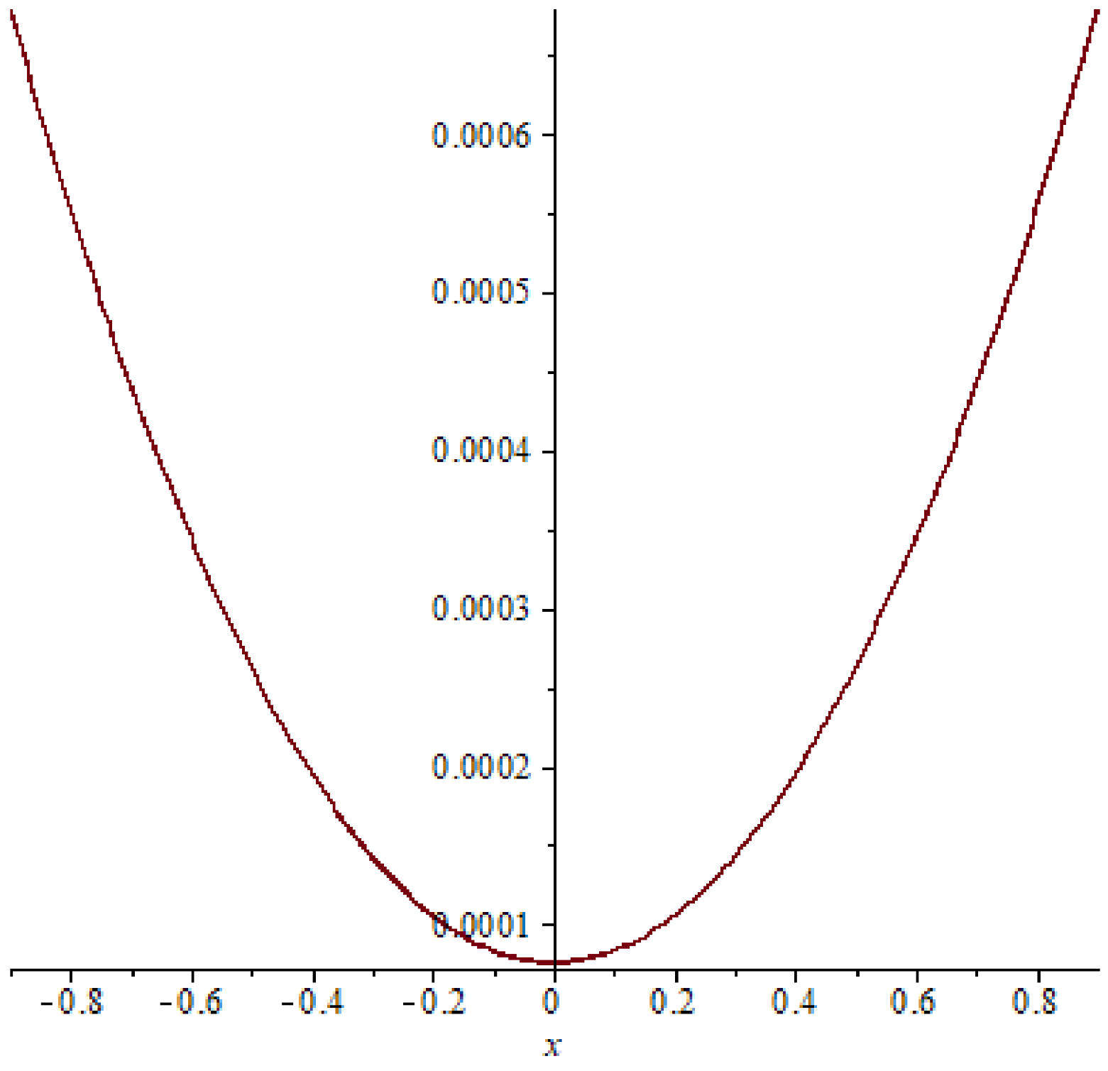
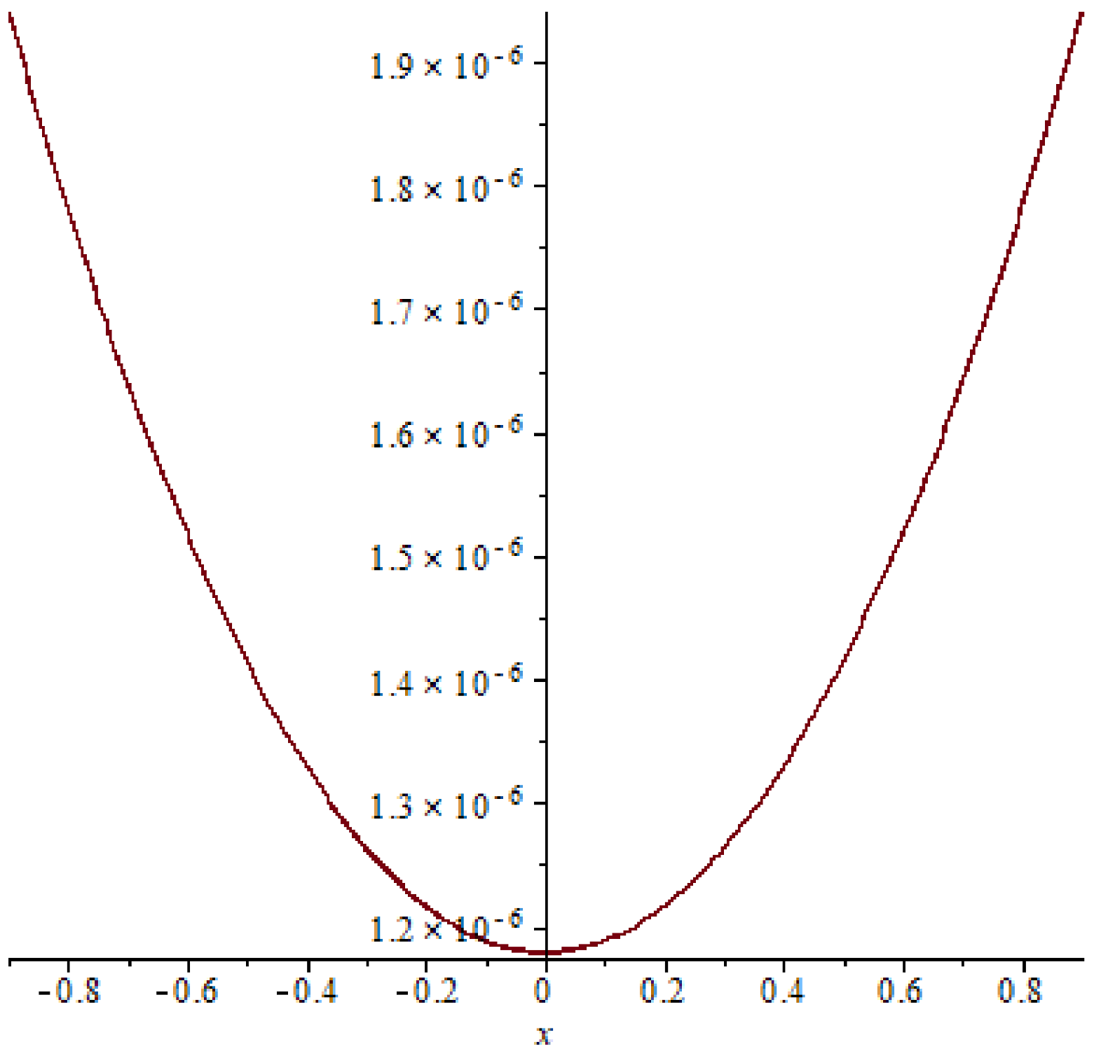
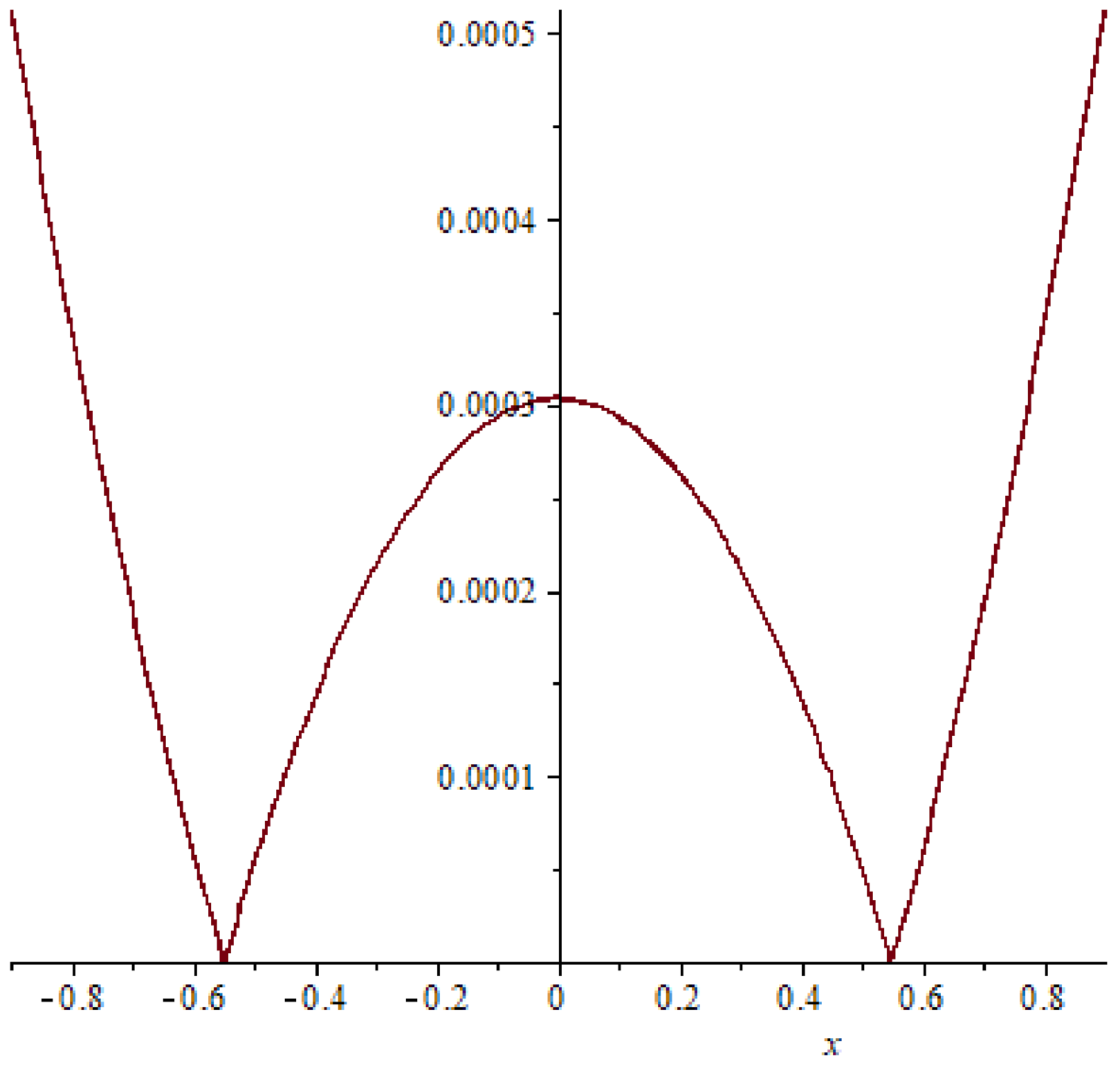
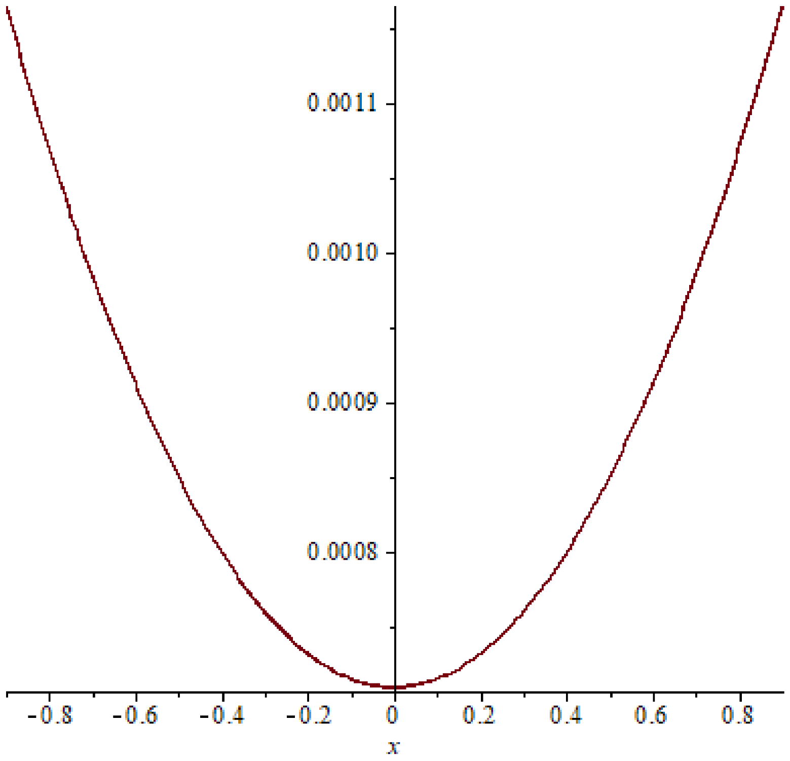
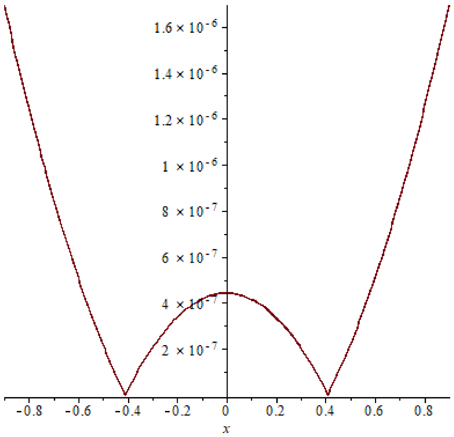
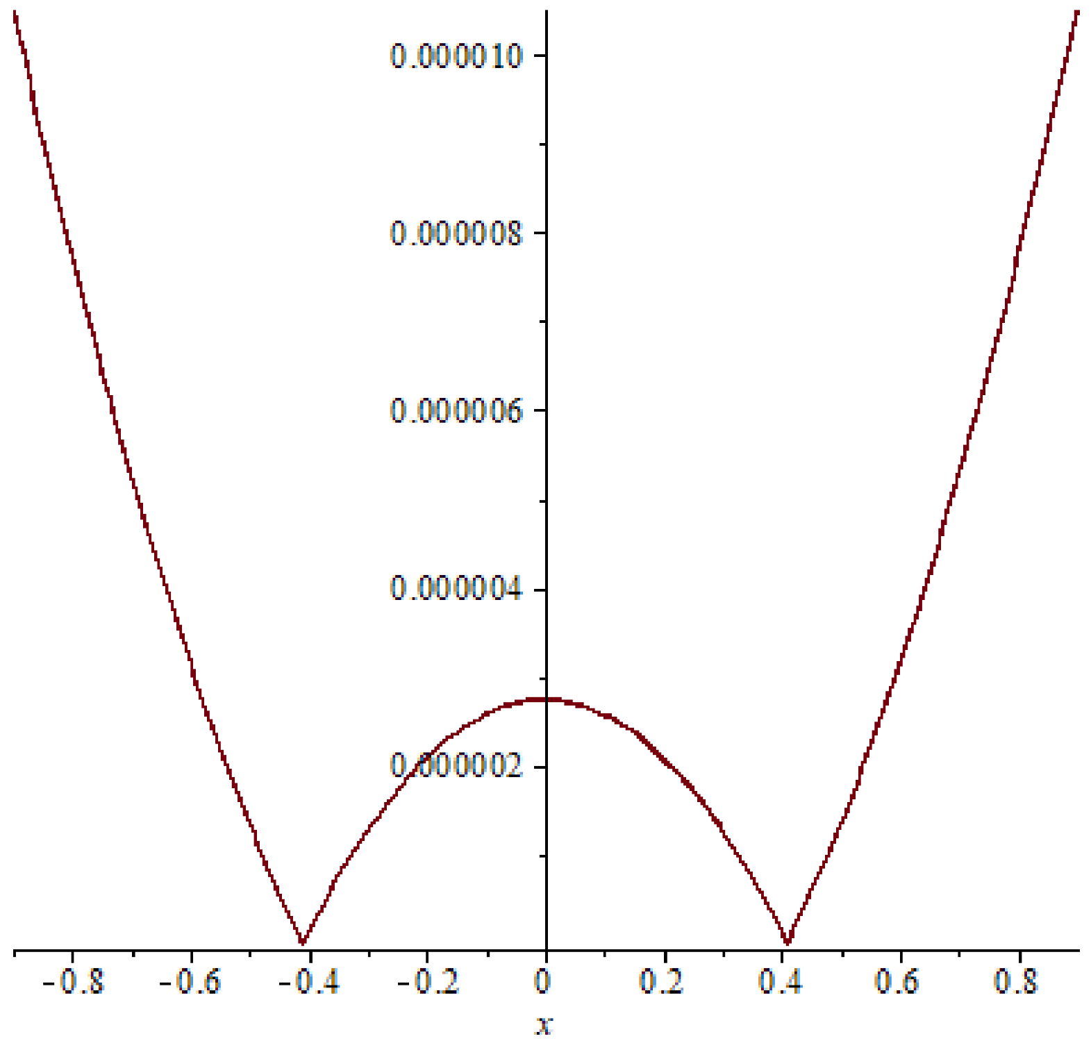
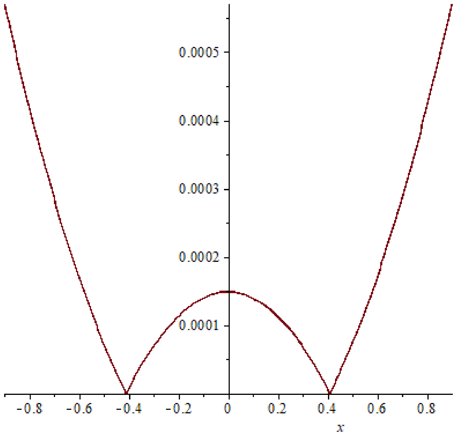
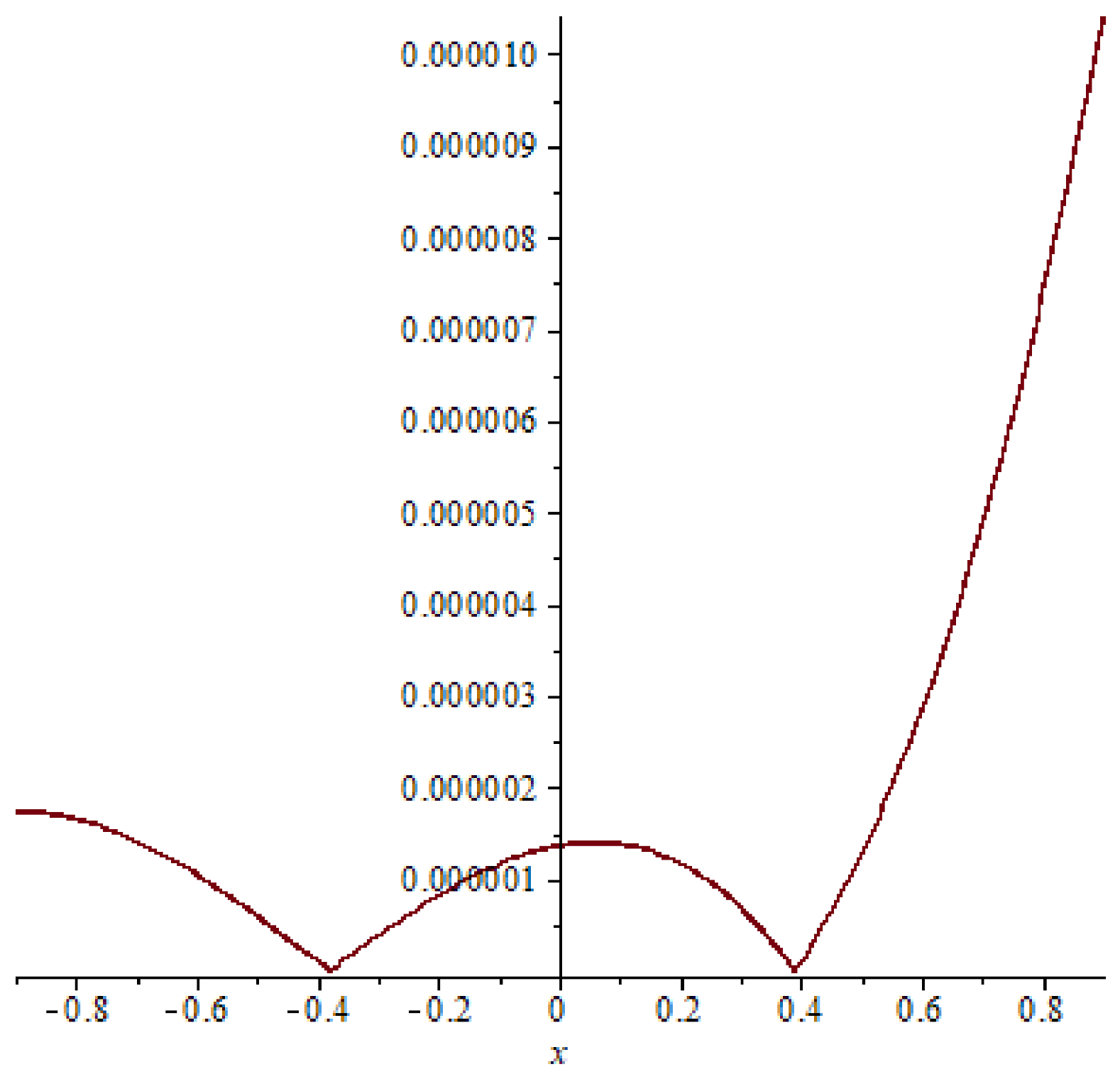
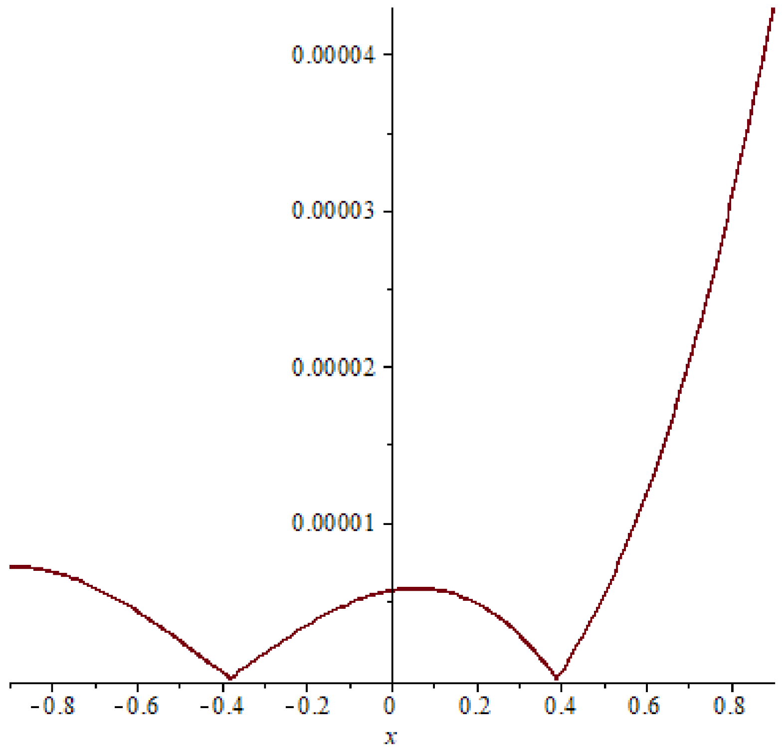
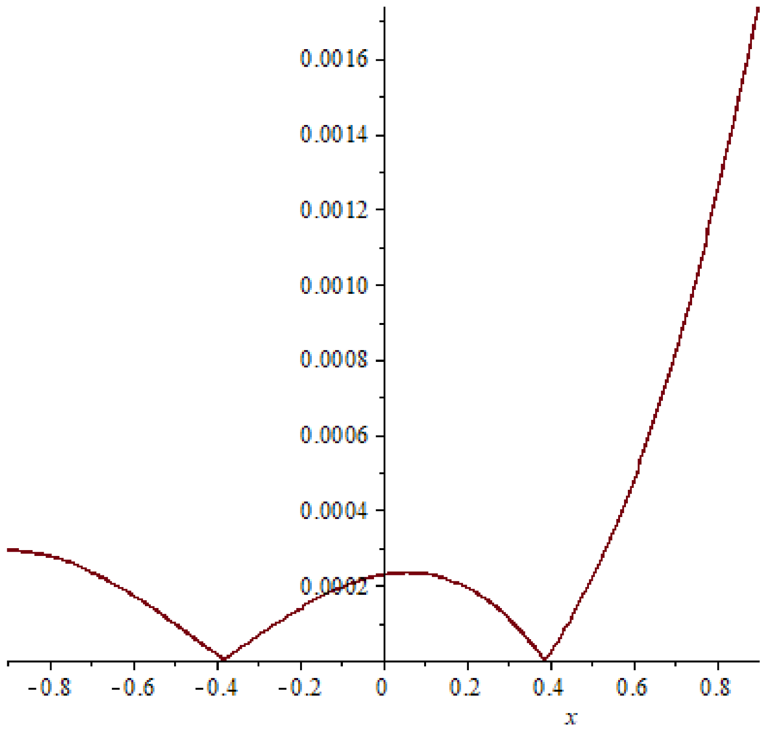
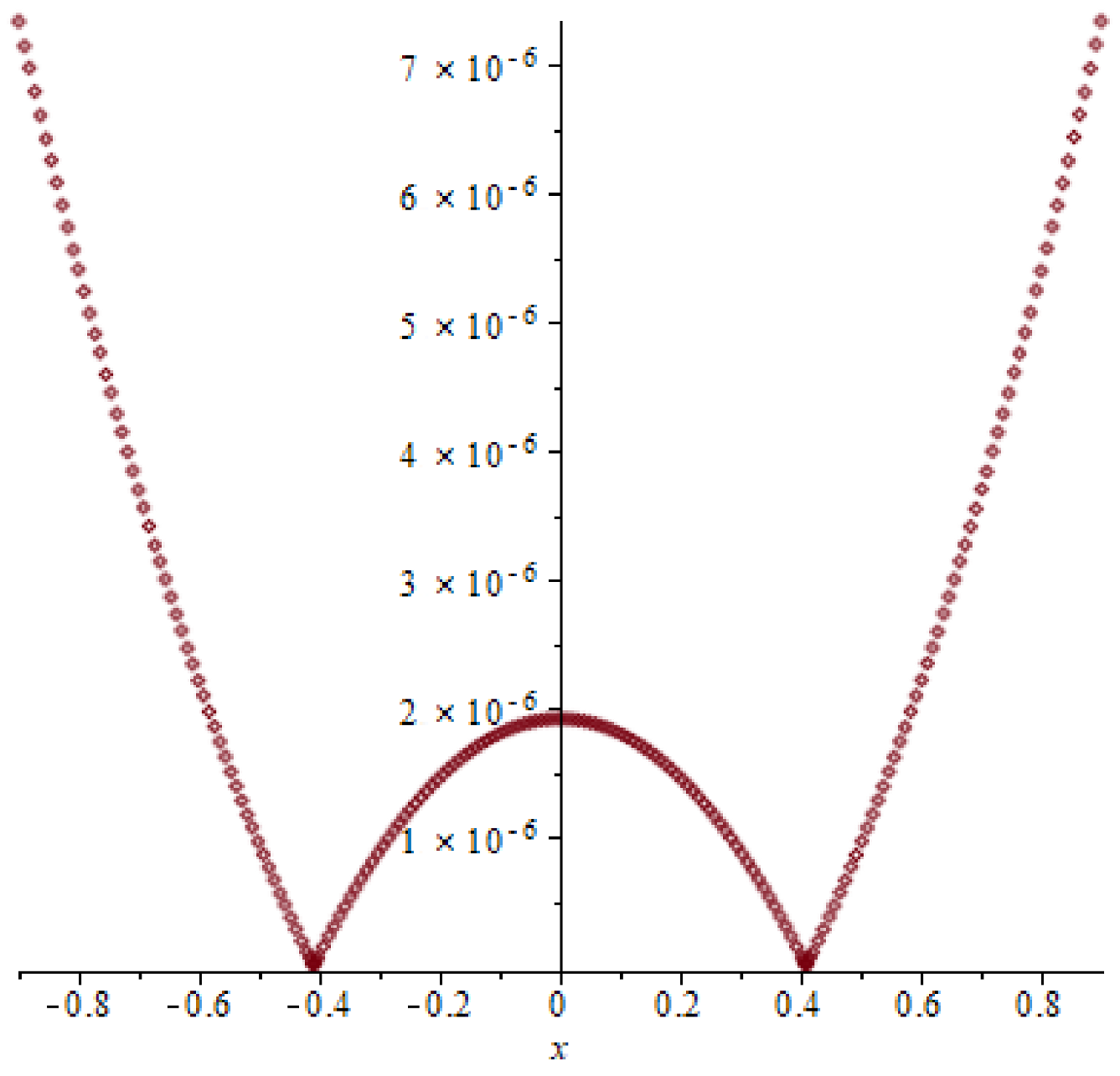
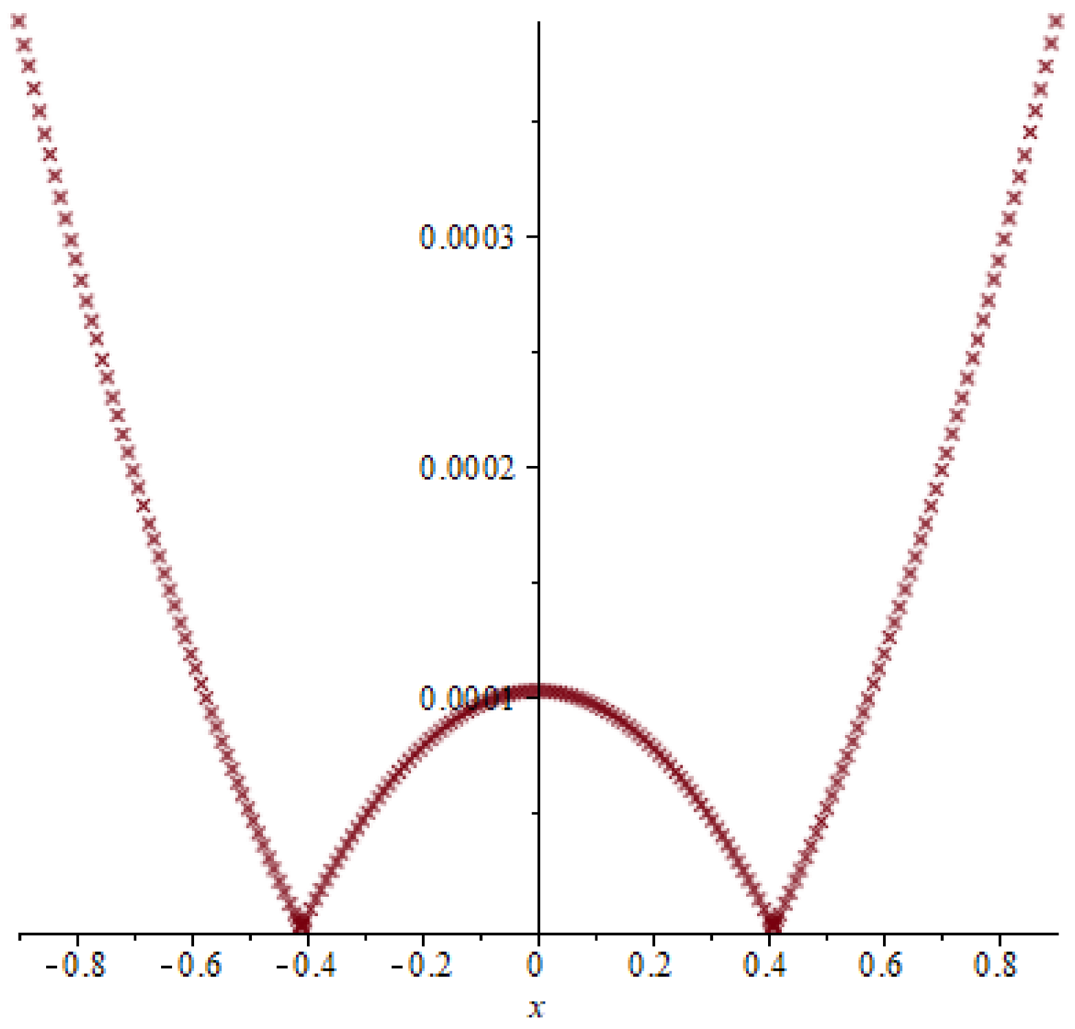
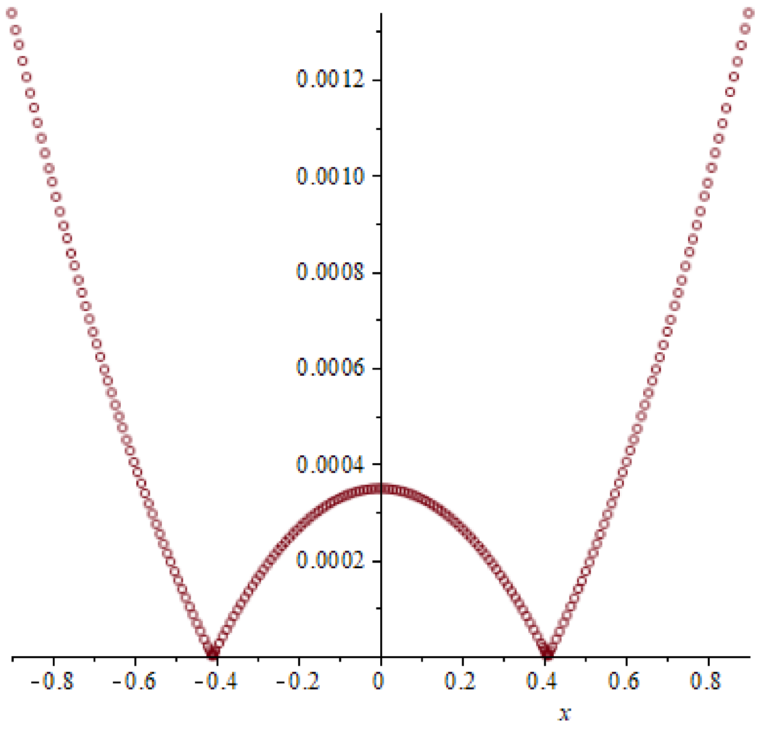
  • Comparison of results: In example (1): It is noticeable in the first example, the first case, that there is a very large convergence between the positive and negative values of the integration region. It is also noted that the lowest numerical value of the error is when
    xT = 0T = 0.2T = 0.4T = 0.6
    0.40 2.268777785 × 10 8 1.805812215 × 10 7 8.861846282 × 10 6
    Also, we notice that the highest value of error is at
    xT = 0T = 0.2T = 0.4T = 0.6
    0.80 1.391215037 × 10 6 1.111946083 × 10 5 5.597684160 × 10 4
In the case of the mixed integral equation of the third kind, we note that: the rate of error change for all values of x is very small, which gives a sign that in the third type, there is a semi-stability in the error value. Also, when the time is increased by a rate of T = 0.2 , we find that the error rate increases by (const × 10 1 ) .
Also, the same remarks were realized in the following example and other examples, and important results can be reached, which is when the solution is in the form of the sum of two functions in time and position, we find that the error in successive times increases. This increase will be somewhat high, especially in the mixed equation of the second kind. As for the mixed equation of the second kind, it is more stable.
Based on the findings and discussion above, we can say the next:
1- 
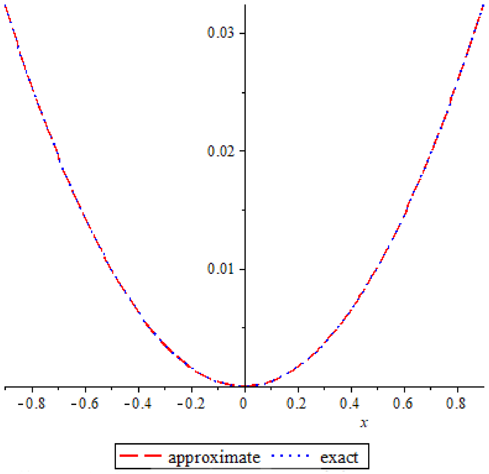
The objective of this article is to obtain a qualitative analysis of the solution of a mixed integral equation having a single kernel in position and another continuous kernel in time. This was done by proving the existence and uniqueness of the solution. In addition, a numerical approach was taken using the Lerch matrix method, which provides a numerical solution in a rapidly converging power series with a computable series under imposed conditions.
2- 
The numerical method used, along with the displacement method, is concentrated in converting the odd integral equations into ordinary integrals that can be easily solved. In addition, the LMC method is very efficient and leads to significant savings in calculation time as well as accuracy in results.
3- 
CPU time in example 1: is 0.09 s, in example 2: is 0.06 s, in example 3: is 0.06 s and the memory: 30.37 M.
4- 
This paper is comprehensive for three types of mixed integral equations, in which mixed integral equations of the first, second and third kind were studied. This complete inclusion of the three types was obtained numerically through the examples mentioned.

10. The Future Work

We will consider the following mixed integro-differential equation:
2 Φ ( x , t ) x 2 c 2 Φ ( x , t ) t = f ( x , t ) + 0 t 0 1 F ( t , τ ) k ( x , y ) Φ ( y , τ ) d y d τ ,
under the conditions
Φ ( 0 , t ) = u 1 ( t ) , Φ ( 1 , t ) = u 2 ( t ) , Φ ( x , 0 ) = u 0 ( x ) .

Author Contributions

Conceptualization, M.A.A.; Methodology, S.E.A., A.M.S.M., M.A.A. and D.S.M.; Software, A.M.S.M., M.A.A. and D.S.M.; Validation, M.A.A.; Formal analysis, S.E.A., A.M.S.M. and D.S.M.; Resources, S.E.A. and M.A.A.; Data curation, A.M.S.M. and D.S.M.; Writing—original draft, S.E.A., A.M.S.M., M.A.A. and D.S.M.; Writing—review & editing, A.M.S.M., M.A.A. and D.S.M.; Project administration, S.E.A.; Funding acquisition, S.E.A. All authors have read and agreed to the published version of the manuscript.

Funding

This research received no external funding.

Data Availability Statement

No instructional records have been created or comfortable with the ongoing assessment data in this original copy.

Acknowledgments

The authors would like to thank the Deanship of Scientific Research at Umm Al-Qura University for supporting this work by Grant Code: (22UQU4282396DSR01).

Conflicts of Interest

No conflict of interest existed when this article’s original draft, publications, or appearance tool place.

References

  1. Jafarian, A.; Nia, S.M.; Golmankhaneh, A.K.; Baleanu, D. On Bernstein Polynomials Method to the System of Abel Integral Equations. Abstr. Appl. Anal. 2014, 2014, 796286. [Google Scholar] [CrossRef]
  2. Noeiaghdam, S.; Micula, S. A novel method for solving second kind Volterra integral equations with discontinuous kernel. Mathematics 2021, 9, 2172. [Google Scholar] [CrossRef]
  3. Nadir, M. Numerical Solution of the Singular Integral Equations of the First Kind on the Curve. Ser. Mat. Inform. 2013, 51, 109–116. [Google Scholar] [CrossRef] [Green Version]
  4. Khairullina, L.E.; Makletsov, S.V. Wavelet-collocation method of solving singular integral equation. Indian J. Sci. Technol. 2017, 10, 1–5. [Google Scholar] [CrossRef] [Green Version]
  5. Gabdulkhaev, B.G.; Tikhonov, I.N. Methods for solving a singular integral equation with cauchy kernel on the real line. Differ. Equ. 2008, 44, 980–990. [Google Scholar] [CrossRef]
  6. Du, J. On the collocation methods for singular integral equations with hilbert kernel. Math. Comput. 2009, 78, 891–928. [Google Scholar] [CrossRef]
  7. Shali, J.A.; Akbarfam, A.J.; Kashfi, M. Application of Chebyshev polynomials to the approximate solution of singular integral equations of the first kind with cauchy kernel on the real half-line. Commun. Math. Appl. 2013, 4, 21–28. [Google Scholar]
  8. Nadir, M. Approximation solution for singular integral equations with logarithmic kernel using adapted linear spline. J. Theor. Appl. Comput. Sci. 2016, 10, 19–25. [Google Scholar]
  9. Mahdy, A.M.S.; Mohamed, D.S. Approximate solution of Cauchy integral equations by using Lucas polynomials. Comput. Appl. Math. 2022, 41, 403. [Google Scholar] [CrossRef]
  10. Seifi, A. Numerical solution of certain Cauchy singular integral equations using a collocation scheme. Adv. Differ. Equ. 2020, 2020, 537. [Google Scholar] [CrossRef]
  11. Seifi, A.; Lotfi, T.; Allahviranloo, T.; Paripour, M. Allahviranloo and M. Paripour. An effective collocation technique to solve the singular Fredholm integral equations with Cauchy kernel. Adv. Differ. Equ. 2017, 2017, 280. [Google Scholar] [CrossRef]
  12. Abdou, M.A.; Raad, S.A.; Wahied, W. Non-Local solution of mixed integral equation with singular kernel. Glob. J. Sci. Front. Res. Math. Decis. Sci. 2015, 15, 1–13. [Google Scholar]
  13. Abdou, M.A.; Al-Kader, G.M.A. Mixed type of integral equation with potential kernel. Turk. J. Math. 2008, 32, 83–101. [Google Scholar]
  14. Abdou, M.A.; Youssef, M.I. A new model for solving three mixed integral equations with continuous and discontinuous kernels. Asian Res. J. Math. 2021, 17, 29–38. [Google Scholar] [CrossRef]
  15. Chokri, C. On the numerical solution of Volterra-Fredholm integral equations with Abel kernel using Legendre polynomials. Int. J. Adv. Sci. Tech. 2013, 1, 404–412. [Google Scholar]
  16. Jan, A.R. An asymptotic model for solving mixed integral equation in position and time. J. Math. 2022, 2022, 8063971. [Google Scholar] [CrossRef]
  17. Jan, A.R. Solution of nonlinear mixed integral equation via collocation method basing on orthogonal polynomials. Heliyon 2022, 8, e11827. [Google Scholar] [CrossRef] [PubMed]
  18. Hazmi, S.E.A. Projection-iterated method for solving numerically the nonlinear mixed integral equation in position and time. J.Umm Al-Qura Univ. Appll. Sci. 2023, 1–8. [Google Scholar] [CrossRef]
  19. Matoog, R.T. Numerical treatment for solving nonlinear integral equation of the second kind. J. Appl. Math. Bioinform. 2014, 4, 33–43. [Google Scholar]
  20. Maleknejad, K.; Rashidinia, J.; Eftekhari, T. A new and efficient numerical method based on shifted fractional-order Jacobi operational matrices for solving some classes of two-dimensional nonlinear fractional integral equations. Numer. Partial. Differ. Equ. 2021, 37, 2687–2713. [Google Scholar] [CrossRef]
  21. Liaqat, M.I.; Akgül, A.; Sen, M.D.L.; Bayram, M. Approximate and exact solutions in the sense of conformable derivatives of quantum mechanics models using a novel algorithm. Symmetry 2023, 15, 744. [Google Scholar] [CrossRef]
  22. Attia, N.; Akgul, A.; Alqahtani, R.T. Extension of the reproducing kernel Hilbert space method’s application range to include some important fractional differential equations. Symmetry 2023, 15, 532. [Google Scholar] [CrossRef]
  23. Azeem, M.; Farman, M.; Akgül, A.; Sen, M.D.L. Fractional order operator for symmetric analysis of cancer model on stem cells with chemotherapy. Symmetry 2023, 15, 533. [Google Scholar] [CrossRef]
  24. Mohamed, D.S. Application of Lerch polynomials to approximate solution of singular fredholm integral equations with cauchy kernel. Appl. Math. Inf. Sci. 2022, 16, 565–574. [Google Scholar]
  25. Çayan, S.; Sezer, M. Lerch matrix collocation method for 2D and 3D Volterra type integral and second order partial integro differential equations together with an alternative error analysis and convergence criterion based on residual functions. Turk. J. Math. 2020, 44, 2073–2098. [Google Scholar] [CrossRef]
  26. Çayan, S.; Sezer, M. A new approximation based on residual error estimation for the solution of a class of unsteady convection-diffusion problem. J. Sci. Arts 2020, 2, 323–338. [Google Scholar]
  27. Çayan, S.; Sezer, M. A novel study based on Lerch polynomials for approximate solutions of pure neumann problem. Int. J. Appl. Comput. Math. 2022, 8, 8. [Google Scholar] [CrossRef]
  28. Branson, D. An extension of stirling numbers. Fibonacci Q. 1996, 34, 213–223. [Google Scholar]
  29. Illie, S.; Jeffrey, D.J.; Corless, R.M.; Zhang, X. Computation of stirling numbers and generalizations. In Proceedings of the 17th International Symposium on Symbolic and Numeric Algorithms for Scientific Computing, Timisoara, Romania, 21–24 September 2015; pp. 57–60. [Google Scholar]
  30. Kruchinin, V.; Kruchinin, D. Explicit formulas for some generalized polynomials. Appl. Math. Inf. Sci. 2013, 7, 2083–2088. [Google Scholar] [CrossRef] [Green Version]
  31. Reynolds, R.; Stauffer, A. The Logarithmic transform of a polynomial function expressed in terms of the Lerch function. Mathematics 2021, 9, 1754. [Google Scholar] [CrossRef]
  32. Balakrishnan, N. Advances in Combinatorial Methods and Applications to Probability and Statistics; Birkhäuser: Basel, Switzerland; Berlin, Germany; Boston, MA, USA, 1997. [Google Scholar]
  33. Mahdy, A.M.S.; Abdou, M.A.; Mohamed, D.S. Computational methods for solving higher-order (1 + 1) dimensional mixed-difference integro-differential equations with variable coefficients. Mathematics 2023, 11, 2045. [Google Scholar] [CrossRef]
Figure 1. The absolute error of example 1 case (11), T = 0.2.
Symmetry 15 01284 g001
Figure 2. The error of example 1 case (11), T = 0.4.
Symmetry 15 01284 g002
Figure 3. The error of example 1 case (11), T = 0.6.
Symmetry 15 01284 g003
Figure 4. The exact and approximate solution of example 1 case (11), T = 0.2.
Symmetry 15 01284 g004
Figure 5. The error of example 1 case (12), T = 0.2.
Symmetry 15 01284 g005
Figure 6. The error of example 1 case (12), T = 0.4.
Symmetry 15 01284 g006
Figure 7. The error of example 1 case (12), T = 0.6.
Symmetry 15 01284 g007
Figure 8. The absolute error of example 2 case (21), T = 0.2.
Symmetry 15 01284 g008
Figure 9. The absolute error of example 2 case (21), T = 0.4.
Symmetry 15 01284 g009
Figure 10. The absolute error of example 2 case (21), T = 0.6.
Symmetry 15 01284 g010
Figure 11. Absolute error of example 2 case (22), T = 0.2.
Symmetry 15 01284 g011
Figure 12. Absolute error of example 2 case (22), T = 0.4.
Symmetry 15 01284 g012
Figure 13. Absolute error of example 2 case (22), T = 0.6.
Symmetry 15 01284 g013
Figure 14. Absolute error of example 3 case (31), T = 0.2.
Symmetry 15 01284 g014
Figure 15. Absolute error of example 3 case (31), T = 0.4.
Symmetry 15 01284 g015
Figure 16. Absolute error of example 3 case (31), T = 0.6.
Symmetry 15 01284 g016
Figure 17. Absolute error of example 3 case (32), T = 0.2.
Symmetry 15 01284 g017
Figure 18. Absolute error of example 3 case (32), T = 0.4.
Symmetry 15 01284 g018
Figure 19. Absolute error of example 3 case (32), T = 0.6.
Symmetry 15 01284 g019
Figure 20. Absolute error of example 4, T = 0.2.
Symmetry 15 01284 g020
Figure 21. Absolute error of example 4, T = 0.4.
Symmetry 15 01284 g021
Figure 22. Absolute error of example 4, T = 0.6.
Symmetry 15 01284 g022
Table 1. Absolute error example 1 case (11).
xAbs Error for T = 0Abs Error for T = 0.2Abs Error for T = 0.4Abs Error for T = 0.6
00 4.939886371 × 10 7 3.947269514 × 10 6      1.984052689 × 10 4
0.2 0 3.761634297 × 10 7 3.005595977 × 10 6      1.510194131 × 10 4
0.4 0 2.268777785 × 10 8 1.805812215 × 10 7      8.861846282 × 10 6
0.6 0 5.664383629 × 10 7 4.527771973 × 10 6      2.280674304 × 10 4
0.8 0 1.391215037 × 10 6 1.111946083 × 10 5      5.597684160 × 10 4
0.2 0 3.761634445 × 10 7 3.005599051 × 10 6      1.510194127 × 10 4
0.4 0 2.268789635 × 10 8 1.805818065 × 10 7      8.861843518 × 10 6
0.6 0 5.664379629 × 10 7 4.527784999 × 10 6      2.280674398 × 10 4
0.8 0 1.391214089 × 10 6 1.111950415 × 10 5      5.597684382 × 10 4
Table 2. Absolute error example 1 case (12).
xAbs Error for T = 0Abs Error for T = 0.2Abs Error for T = 0.4Abs Error for T = 0.6
00 4.50173876 × 10 6 1.303309878 × 10 5      4.891097646 × 10 4
0.2 0 2.108866596 × 10 6 1.121628678 × 10 5      4.207115091 × 10 4
0.4 0 1.084940436 × 10 6 5.765850778 × 10 6      2.155167447 × 10 4
0.6 0 6.216050828 × 10 7 3.318209226 × 10 6      1.264745255 × 10 4
0.8 0 3.010770441 × 10 6 1.603589323 × 10 5      6.052622984 × 10 4
0.2 0 2.108862756 × 10 6 1.21628678 × 10 5      4.207115081 × 10 4
0.4 0 1.084933716 × 10 6 5.765850782 × 10 6      2.155167365 × 10 4
0.6 0 6.216127652 × 10 7 3.318209214 × 10 6      1.264745533 × 10 4
0.8 0 3.010776207 × 10 6 1.603589321 × 10 5      6.052623644 × 10 4
Table 3. Absolute error example 2 case (21).
xAbs Error for T = 0Abs Error for T = 0.2Abs Error for T = 0.4Abs Error for T = 0.6
00 1.8514 × 10 7 1.001730 × 10 4      7.56408 × 10 5
0.2 0 2.591481852 × 10 7 7.722117710 × 10 5      1.054254995 × 10 4
0.4 0 4.812134813 × 10 7 8.365576795 × 10 6      1.947796361 × 10 4
0.6 0 8.513369995 × 10 7 1.063938183 × 10 4      3.437032069 × 10 4
0.8 0 1.369519851 × 10 6 2.670570256 × 10 4      5.521962090 × 10 4
0.2 0 2.591878148 × 10 7 7.722106290 × 10 5      1.054255405 × 10 4
0.4 0 4.812905187 × 10 7 8.365383205 × 10 6      1.947797239 × 10 4
0.6 0 8.514470005 × 10 7 1.063940217 × 10 4      3.437033531 × 10 4
0.8 0 1.369656149 × 10 6 2.670571344 × 10 4      5.521964310 × 10 4
Table 4. Absolute error example 2 case (22).
xAbs Error for T = 0Abs Error for T = 0.2Abs Error for T = 0.4Abs Error for T = 0.6
00 1.17851 × 10 6 3.033303 × 10 4      7.093212 × 10 4
0.2 0 1.216148624 × 10 6 2.630243409 × 10 5      7.317845839 × 10 4
0.4 0 1.329058991 × 10 6 1.421065469 × 10 4      7.991747752 × 10 4
0.6 0 1.517232844 × 10 6 5.942307666 × 10 5      9.114917731 × 10 4
0.8 0 1.780661928 × 10 6 3.415645247 × 10 4      1.068735577 × 10 3
0.2 0 1.216151376 × 10 6 2.630244191 × 10 4      7.317846241 × 10 4
0.4 0 1.329081009 × 10 6 1.421066931 × 10 4      7.991748568 × 10 4
0.6 0 1.517307156 × 10 6 5.942288334 × 10 5      1.14918989 × 10 4
0.8 0 1.780838072 × 10 6 3.415643153 × 10 4      1.068735751 × 10 4
Table 5. Absolute error example 3 case (31).
xAbs Error for T = 0Abs Error for T = 0.2Abs Error for T = 0.4Abs Error for T = 0.6
00 4.423262230 × 10 7 2.741292043 × 10 6      1.487028118 × 10 4
0.2 0 3.368245381 × 10 7 2.087407130 × 10 6      1.132067839 × 10 4
0.4 0 2.032474385 × 10 8 1.257487377 × 10 7      6.718700750 × 10 6
0.6 0 5.071712691 × 10 7 3.143688612 × 10 6      1.707614370 × 10 4
0.8 0 1.245661610 × 10 6 7.720910399 × 10 6      4.192336286 × 10 4
0.2 0 3.368279079 × 10 7 2.087408956 × 10 6      1.132067837 × 10 4
0.4 0 2.032770215 × 10 8 1.257633483 × 10 7      6.718698850 × 10 6
0.6 0 5.071762849 × 10 7 3.143639302 × 10 6      1.707614434 × 10 4
0.8 0 1.245685944 × 10 6 7.720793515 × 10 6      4.192336438 × 10 4
Table 6. Absolute error example 3 case (32).
xAbs error for T = 0Abs Error for T = 0.2Abs Error for T = 0.4Abs Error for T = 0.6
00 1.361106516 × 10 6 5.618946143 × 10 6      2.73852223 × 10 4
0.2 0 1.172489734 × 10 6 4.838795847 × 10 6      1.954927116 × 10 4
0.4 0 1.066157435 × 10 7 4.42568224 × 10 7      1.833811114 × 10 5
0.6 0 2.832866610 × 10 6 1.169657584 × 10 5      4.734171421 × 10 4
0.8 0 7.362919560 × 10 6 3.039465679 × 10 5      1.229054277 × 10 3
0.2 0 8.158912984 × 10 7 3.369312439 × 10 6      1.366493170 × 10 4
0.4 0 1.064992245 × 10 7 4.38675490 × 10 7      1.740510826 × 10 5
0.6 0 1.049408358 × 10 6 4.333587872 × 10 6      7.54681573 × 10 4
0.8 0 1.656179408 × 10 6 6.84399493 × 10 6      2.782299342 × 10 4
Table 7. Absolute error example 4.
xAbs Error for T = 0Abs Error for T = 0.2Abs Error for T = 0.4Abs Error for T = 0.6
00 1.914508119 × 10 6 1.026585542 × 10 4      3.486476949 × 10 4
0.2 0 1.457667893 × 10 6 7.816842988 × 10 5      2.653904758 × 10 4
0.4 0 8.754630969 × 10 8 4.698119601 × 10 6      1.561886202 × 10 5
0.6 0 2.195857987 × 10 6 1.77524026 × 10 4      4.006671411 × 10 4
0.8 0 5.392546355 × 10 6 2.891831626 × 10 5      9.834675281 × 10 4
0.2 0 1.458068345 × 10 6 7.816851852 × 10 5      2.653905140 × 10 4
0.4 0 8.834992831 × 10 8 4.698348799 × 10 6      1.561892778 × 10 5
0.6 0 2.194645775 × 10 6 1.177519290 × 10 4      4.006670691 × 10 4
0.8 0 5.390917407 × 10 6 2.891822890 × 10 4      9.834674821 × 10 4
Disclaimer/Publisher’s Note: The statements, opinions and data contained in all publications are solely those of the individual author(s) and contributor(s) and not of MDPI and/or the editor(s). MDPI and/or the editor(s) disclaim responsibility for any injury to people or property resulting from any ideas, methods, instructions or products referred to in the content.

