Estimation of Lamb Wave Anti-Symmetric Mode Phase Velocity in Various Dispersion Ranges Using Only Two Signals

Abstract

The application of non-stationary Lamb wave signals is a promising tool in various industrial applications where information about changes inside a structure is required. Phase velocity is one of the Lamb wave parameters that can be used for inhomogeneities detection. The possibility of reconstructing the segment of the phase velocity in a strong dispersion range using only two signals is proposed. The theoretical study is performed using signals of the A₀ mode propagating in an aluminium plate at a frequency of 150 kHz, 300 kHz, 500 kHz and 900 kHz. The experiment was carried out at a value of 300 kHz. The studies conducted indicated that the maximum distance between two signals, at which the time-of-flight can be measured between the same phase points, is the main parameter for the two signals technique application. Theoretical and experimental studies were performed, and the mean relative error was calculated by comparing the obtained results with those calculated via the SAFE method. In the theoretical study, the mean relative error of 0.33% was obtained at 150 kHz, 0.22% at 300 kHz, 0.23% at 500 kHz and 0.11% at 900 kHz. The calculated mean relative errors ${\delta }_{c_{ph}}=0.91\%$ and ${\delta }_{c_{ph}}=1.36\%$ were obtained at different distances in the experimental study. The results obtained show that the estimation of the phase velocity in dispersion ranges using only two received signals was a useful tool that saved time and effort.

1. Introduction

The Lamb waves, which propagate within structures, are a well-known technique for Non-Destructive Testing (NDT) and Structural Health Monitoring (SHM) [1,2,3]. There are two groups of dispersive modes of Lamb waves: symmetric S_n and anti-symmetric A_n [4,5]. The signals of the anti-symmetric and symmetric modes have different wavelengths depending on the frequency; therefore different sizes of defects can be detected. Since the signals of these modes are highly sensitive to material properties, the detection and evaluation of various cracks at different depths, heterogeneities, material fatigue, etc., could be determined [1,3]. Therefore, various types of objects can be inspected for internal defects using different symmetric S_n and anti-symmetric A_n modes of Lamb waves [1].

However, the real-time testing of objects remains a complex and challenging task due to the multi-modal nature, dispersive phenomenon, multi-path characteristics of Lamb waves and sensitivity to environmental and operational conditions (EOCs) parameters [6,7,8]. Thus, one of the main reasons that complicates the application of these waves is the dispersion phenomenon [2,4,9]. The non-stationary Lamb wave signal packets consist of frequency components that propagate at different velocities [10] and are characterized by phase and group velocities. These velocities are described by dispersion curves, which vary depending on frequency (f) and object thickness (d) [4,11,12]. Since the effect of dispersion is a function of distance, it affects the signal’s temporal spreading duration and decreases signal amplitude depending on the distance [4,13,14]. Therefore, the signal processing methods (SPMs) that can evaluate the dispersion phenomenon and relate the frequency with phase and group velocities should be used in the Lamb wave applications. Thus, due to the dispersion phenomenon, the application of such waves requires new or adapted SPMs that should perform phase and group velocity estimation, relate them to frequencies, and reconstruct the dispersion curves. Recently, considerable efforts have been made to develop digital SPMs that are more suitable for the display, analysis and processing of non-stationary signals. A number of signal processing techniques were adapted and used to estimate phase and group velocities; these techniques include the two-dimensional fast Fourier transform (2D-FFT) and variations, Wavelet Transform (WT), Wigner-Ville Distribution (WVD) and variations and others [13,15,16,17,18]. However, to obtain a reliable fragment of the dispersion curve due to the dispersion phenomenon, all these techniques require the acquisition of signals at many points along the wave propagation path, which is time-consuming and laborious. Therefore, new solutions that save time and effort are being sought. One of the recently proposed solutions is the reconstruction of the phase velocity dispersion curves using two received signals. Zeng et al. have proposed the use of the short-time chirp-Fourier transform (STCFT) method [19,20], and Crespo et al. have proposed a method based on the Hilbert transformation and cross-correlation techniques implemented together [21]. However, the authors recognize that reconstructing the phase velocity segment in a strong dispersion range using only two received signals is a difficult task. Therefore, the proposed methods have limitations of one kind or other, such as the requirement for a specific signal generation when using a chirp signal for Lamb wave generation, the need to achieve high resolution in both the time and frequency domains simultaneously [19] or the technique’s high sensitivity to mode shape distortions [21]. All of these limitations affect the accuracy of the final results and complicate measurements.

A two-signal analysis method using a hybrid zero-crossing technique implemented together with a spectrum decomposition technique was proposed to estimate the phase velocity dispersion of Lamb waves [22]. This proposed technique is already used by other authors to detect corrosion degradation of ageing structural components [23] and for corrosion degradation monitoring of ship-stiffened plates [11]. However, using such a hybrid technique, when the received signals are filtered, it is impossible to determine the main parameters and regularities required for the estimation of the phase velocity in a strongly dispersive medium. Thus, a method should be used that allows the identification of the necessary information.

The zero-crossing method has been proposed and applied for the phase velocity dispersion evaluation of anti-symmetric A₀ and symmetric S₀ modes of Lamb waves. A description of the algorithm using a set of signals has been provided in our previous work [10]. The results obtained indicated that the zero-crossing technique was a good tool for the phase velocity dispersion evaluation using a set of signals. Since it was found that the main requirement for determining the phase velocity is that the time-of-flight must be measured between the same phase points between the two selected signals, the maximum possible distance between the two received signals should be known [22]. Therefore, a deeper analysis and explanation is necessary in order to understand these waves feature and how to perfume the evaluation of the phase velocity in a strong dispersion range using only two measured signals.

The objective of this work is to present the essential parameters and regularities needed to evaluate the phase velocity of the anti-symmetric Lamb wave mode in various dispersive ranges using only two signals. We also aim to identify the key constraints involved in evaluating the phase velocity in the dispersive range and propose methods to overcome these challenges, to perform a verification using analytically calculated and experimentally measured signals at different propagation distances, calculating the mean relative error.

2. Phase Velocity Evaluation in Dispersive Media

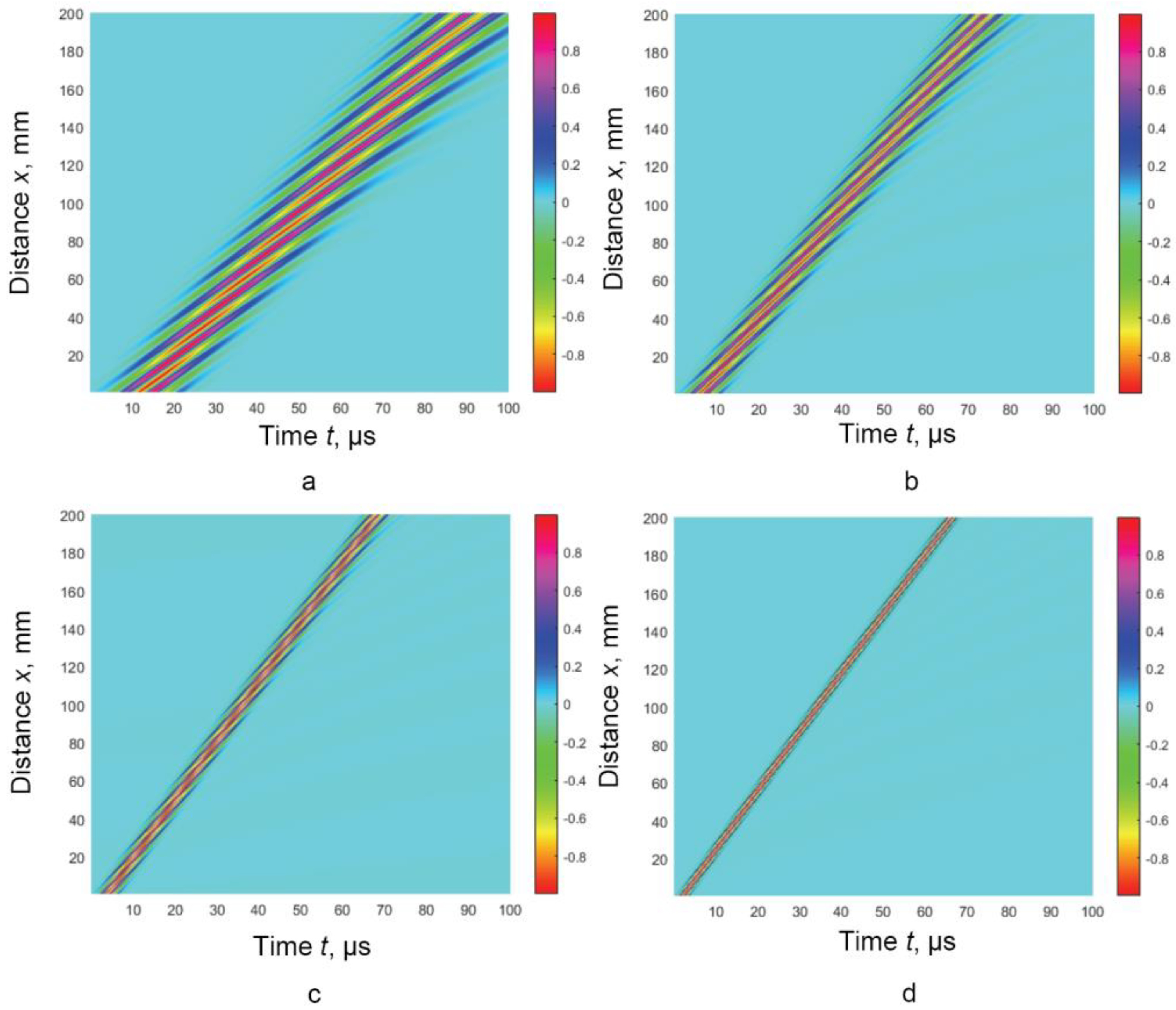
2.1. Analytical Calculation of Propagating Wave Signals

In order to perform a deeper analysis and explain the phase velocity characteristics of the Lamb wave modes in the dispersion range, a simplified aluminium plate with a thickness of 2 mm was selected for the study. The material properties of the aluminium plate are: density ρ = 2780 kg/m³, Young modulus E = 71.78 GPa and Poisson’s ratio ν = 0.3435. According to the presented object parameters, the phase and group velocities dispersion curves of the A₀ mode of Lamb waves were calculated using the SAFE method [24,25] (Figure 1).

The calculated phase and group velocities dispersion curves indicate that the anti-symmetric A₀ mode possesses a strong dispersion within the frequency range of 100 to 1000 kHz. Thus, in order to explain the peculiarities of the signal propagation in the dispersive medium and to determine main rules required for the phase velocity evaluation, different frequency ranges were chosen for the study: 150 kHz, 300 kHz, 500 kHz and 900 kHz. Thus, the sets of simulated signals of the A₀ mode at various frequency ranges were obtained applying the simplified complex transfer function of the Lamb waves propagating in a selected aluminium plate [26]:

$$u\left(x,t\right)=\frac{1}{2\pi }\underset{-\infty }{\overset{\infty }{\int }}\mathrm{F}\mathrm{T}\left(u_0\left(t\right)\right)e^{-j\omega \frac{x}{c_p\left(\omega \right)}}{e}^{j\omega t}d\omega$$

(1)

where u₀(t) is the excitation signal, FT is the Fourier transform, t is the time, ω = 2πf is the angular frequency, x is the propagation distance, f is the frequency, j is the basic imaginary unit $j=\sqrt{-1}$. Since the attenuation of Lamb waves propagating in metal plates is very low, this parameter is neglected.

The excitation signals u₀(t) of three-period with 150 kHz, 300 kHz, 500 kHz and 900 kHz harmonic bursts with a Gaussian envelope were used as the incident signals. The received signals u(x,t) of A₀ mode of Lamb waves were calculated at a distance from 0 mm to 2000 mm with a scanning step of Δx = 0.1 mm. In this way, a set of 2001 simulated signals were obtained in each analysis case. The B-scan images at different frequency ranges of the A₀ mode are presented in Figure 2a–d.

The B-scan images show that the phase velocity values are different for different frequency ranges. Since the zero-crossing technique was presented and used in our previous works [10,22], this method was selected and applied for the determination of regularities of signals propagating in a dispersed medium and the estimation of phase velocity.

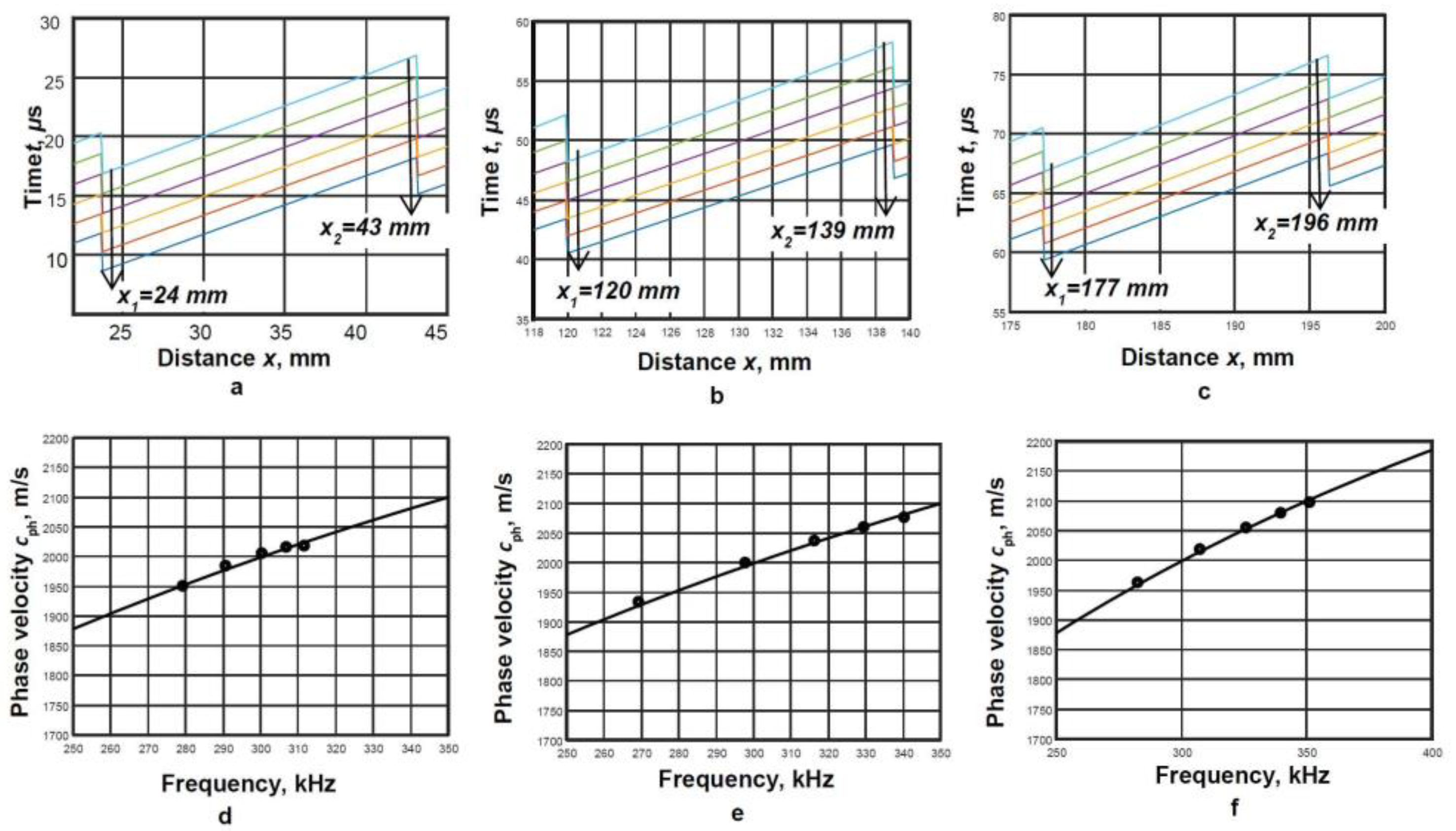
2.2. Zero Crossing Technique

The zero-crossing algorithm was presented in our previous work [10]. However, in order to calculate the phase velocity dispersion curve as accurately as possible using only two signals, some changes to the algorithm are required. So, the zero-crossing algorithm can be divided in to three main parts.

The first part involves the calculation of the phase velocity values, the second part is related to calculation of frequency values, and the third part is concerned with the reconstruction of the phase velocity dispersion curves. A brief description of the algorithm is presented below.

• The phase velocity calculation

The selection of the threshold level U_L;

Time instants at which both signals $u_{x1}\left(t\right)$ and $u_{x2}\left(t\right)$ cross the zero-amplitude line $t_1\left(x_1\right)$, $t_2\left(x_1\right)$, …, $t_N\left(x_1\right)$ and $t_1\left(x_2\right)$, $t_2\left(x_2\right)$, …, $t_N\left(x_2\right)$ are measured;

The phase velocity values are calculated using the expression:

$$c_{ph,k\left(x_1\right)}=\frac{∆x}{t_k\left(x_1+∆x\right)-t_k\left(x_1\right)},$$

(2)

where $∆x=x_2-x_1$, k = 1,2, …, N, k—the number of zero-crossing instant in the signals, N—the total number of measured zero-crossing instants in the signals.

• The calculation of frequency

The duration of each selected half-periods $T_{\mathrm{0.5,1}}\left(x_1\right)$, $T_{\mathrm{0.5,2}}\left(x_1\right)$, …, $T_{0.5,N-1}\left(x_1\right)$ and $T_{\mathrm{0.5,1}}\left(x_2\right)$, $T_{\mathrm{0.5,2}}\left(x_2\right)$, …, $T_{0.5,N-1}\left(x_2\right)$ are calculated by:

$$\begin{gathered} T_{0.5,k}\left(x_1\right)=t_{k+1}\left(x_1\right)-t_k\left(x_1\right), \\ {T}_{0.5,k}\left(x_2\right)=t_{k+1}\left(x_2\right)-t_k\left(x_2\right) \end{gathered}$$

(3)

The equivalent frequencies corresponding to the calculated duration of each selected half-period for each signal are estimated by:

$$f_{\mathrm{0,5},k\left(x_1\right)}=\frac{1}{{2·T}_{0.5k}\left(x_1\right)}, f_{\mathrm{0,5},k\left(x_2\right)}=\frac{1}{{2·T}_{0.5k}\left(x_2\right)},$$

(4)

Determination of the frequency values ($f_{\mathrm{0,5},ki}$) for the dispersion curve reconstruction:

$$f_{\mathrm{0,5},ki}=\frac{f_{\mathrm{0,5},k\left(x_1\right)}+f_{\mathrm{0,5},k\left(x_2\right)}}{2}$$

(5)

• The segments of the phase velocity dispersion curve are described by creating sets of pairs of frequencies f_ki and determined phase (c_ph,k) velocities:

$$\left\{{f_{ki},c}_{ph,k}\right\},$$

(6)

So, the phase velocity values were estimated from time delay measurements between two registered signals at different spatial positions of known distance and equivalent frequency values are calculated using the same registered signals. Therefore, the uniqueness of the proposed technique is that it requires only a few zero-crossing instants, measured according to half of the periods of a particular mode signal, to reconstruct its frequency values. In this way, the segments of the phase velocity dispersion curves of Lamb waves are reconstructed.

2.3. Phase Velocity Features in Dispersion Range

In order to explain the peculiarities of signal propagation in a dispersive medium, the obtained set of the A₀ mode signals at 300 kHz frequency is used. Using the presented zero-crossing algorithm, the threshold level U_L = 0.1 is set and one time instant at which the signal crosses the zero-amplitude line is determined in Figure 3a. Figure 3b shows the distribution of the zero-crossing instants of the signal in the whole propagation distance and the zoom-in point shows the analysed area from 138 mm to 164 mm. In order to explain Figure 3b, tree signals of the A₀ mode at different distances: 139 mm, 158 mm and 162 mm were selected for the study, which are presented in Figure 3c–e, accordingly.

Thus, using the selected U_L = 0.1 for each analysed signal, one time instant at which the signals cross the zero-amplitude line is determined (Figure 3c–e).

According to the algorithm, each signal is divided into half periods that show the location of the first-time instant. These set points are used for the phase velocity evaluation. Therefore, it is very important to use set points that are in the same half period of the signals for the phase velocity calculation. However, due to the selected threshold level and dispersion nature of the Lamb waves, which influence the signal form changes, the first-time instant, which crosses the zero-amplitude line, is determined in different half-periods. As shown in Figure 3c,d, the first-time instant, which crosses the zero-amplitude line, is located in the second half-period of the signals at distances of 139 mm and 158 mm; meanwhile, the first-time instant is determined in the first half-period of the signal at the distance of 160 mm (Figure 3e). Thus, depending on the signal amplitude changes and selected threshold level, the first zero-crossing points of the signals are determined at different half-periods of the signal, depending on the propagation distances. In this way, the time-of-flight is evaluated between the phase points, which are in the different half-periods, and that means that these phase points are not the same. So, it is assumed that the time-of-flight between two signals at the distances of 139 mm and 160 mm should be determined incorrectly; meanwhile, at the distances of 139 mm and 158, it should be determined correctly. In order to confirm this regularity, the phase velocity values are calculated by applying the zero-crossing technique and using six-time instants at which the signals cross the zero-amplitude line. Figure 4a shows the distribution of six zero-crossing instants of the signals in the whole propagation distance, and Figure 4b shows the analysed area from 135 mm to 160 mm. The calculated phase velocity results are presented in

Table 1. The calculated phase velocity results using calculated signals at different distances.

Zero-Crossing Point	I	II	III	IV	V	VI
x1 = 139 mm; x2 = 158 mm
$c_{ph}$, m/s	2092	2077	2058	2059	1984	1905
x1 = 139 mm; x2 = 160 mm
$c_{ph}$, m/s	2757	2755	2754	2750	2741	2724

.

The phase velocity value is obtained around 2000 m/s using selected signals at distances of 139 mm and 158 mm (

Table 2. The calculated results of the mean relative error ${\delta }_c{}_{ph}$ using a pair of the signals at different distances.

Distance of the signals, mm	x1 = 24; x2 = 43	x1 = 120; x2 = 139	x1 = 177; x2 = 196
${{\delta }_c}_{ph}$, %	0.22	0.22	0.2

). The obtained different phase velocity values indicate the distribution and propagation of different frequency components in different parts of the signal [10]. The results obtained using signals at distances of 139 mm and 160 mm indicate that the time-of-flight in each half-period was determined incorrectly, therefore, the phase velocity values were calculated incorrectly. The resulting signature of the A₀ mode in the dispersion range shows that the phase velocity estimation using only two signals has a distance limit. Thus, to avoid this limitation, it is necessary to use a set of signals to estimate the phase velocity in the dispersion ranges using conventional signal processing techniques. However, it is possible to calculate the maximum possible distance between two signals and estimate the phase velocity using only the two measured signals. A study to estimate the phase velocity in the strong dispersive range using only two signals is presented in the next section.

2.4. Evaluation of the Phase Velocity Using Two Signals

2.4.1. Evaluation of the Phase Velocity at 300 kHz Frequency Range

The theoretical study was performed using simulated signals of the A₀ mode, which are presented in a B-scan image (Figure 2b). The phase velocity was calculated by applying the zero-crossing technique, using the threshold level U_L = 0.1 and six-times instants at which the signal crosses the zero-amplitude line were chosen, as shown in Figure 4a. In order to demonstrate the reconstruction of the phase velocity dispersion curve within the dispersion range using only two signals, a study was performed using signal pairs at different propagation distances. The maximal distance $∆l$ between two signals could be determined from the dispersion curves of the phase and group velocities and calculated according to:

$$∆l<\frac{1}{f}\frac{\left(c_{ph·}\right(f\left)c_{gr}\right(f\left)\right)}{\left|c_{gr}\left(f\right)-c_{ph\left(f\right)}\right|},$$

(7)

where f is the central frequency, $c_{gr}$ and $c_{ph}$ are the group and phase velocities, accordingly, of the Lamb wave A₀ mode in the frequency range during the analysis.

The maximal distance between two signals at which the time-of-flight can be measured between the same phase points for the A₀ mode at 300 kHz frequency is $∆l$= 20 mm. In order to demonstrate the effectiveness of the method, three different distances were chosen for the study, which are presented in Figure 5a–c. The first selected distance was from 24 mm up to 43 mm, as shown in Figure 5a, the second from 120 mm up to 139 mm, shown in Figure 5b and the third from 177 mm up to 196 mm, as shown in Figure 5c. Thus, the signals x₁ = 24 mm and x₂ = 43 mm, x₁ = 120 mm and x₂ = 139 mm and x₁ = 177 mm and x₂ = 196 mm were selected for the segment of phase velocity dispersion curve reconstruction. In order to verify the suitability of the method for reconstructing phase velocity dispersion curves using only two signals, the obtained results were compared with the dispersion curve calculated by the SAFE method, and the mean relative error was calculated, in each case, according to:

$${\delta }_{c_{ph}}=100\mathrm{\%}·\frac{1}{\mathrm{N}}{\sum }_{n=1}^{\mathrm{N}}\frac{\left|c_{ph,n}-c_{ph,n}^{\mathrm{S}\mathrm{A}\mathrm{F}\mathrm{E}}\right|}{c_{ph,n}^{\mathrm{S}\mathrm{A}\mathrm{F}\mathrm{E}}}.$$

(8)

where $c_{ph,n}$ is the values of the phase velocity calculated by the presented algorithm, $c_{ph,n}^{\mathrm{S}\mathrm{A}\mathrm{F}\mathrm{E}}$ is the value of the phase velocity calculated by the SAFE method. The reconstructed segments of the phase velocity dispersion curves of the A₀ mode, using pair of the signals at different distances, are compared with those calculated by the SAFE method and presented in Figure 5d–f, respectively. The calculated results of the mean relative error ${\delta }_{c_{ph}}$ are presented in Table 2.

The calculated mean relative error of the phase velocity (Table 2) obtained in each selected case was around 0.22%. The results obtained in the 300 kHz frequency range, using pairs of signals at varying distances, demonstrate that reconstructing phase velocity in the dispersion range was an achievable task. Consequently, to validate these results, the proposed technique should be tested across different dispersion ranges.

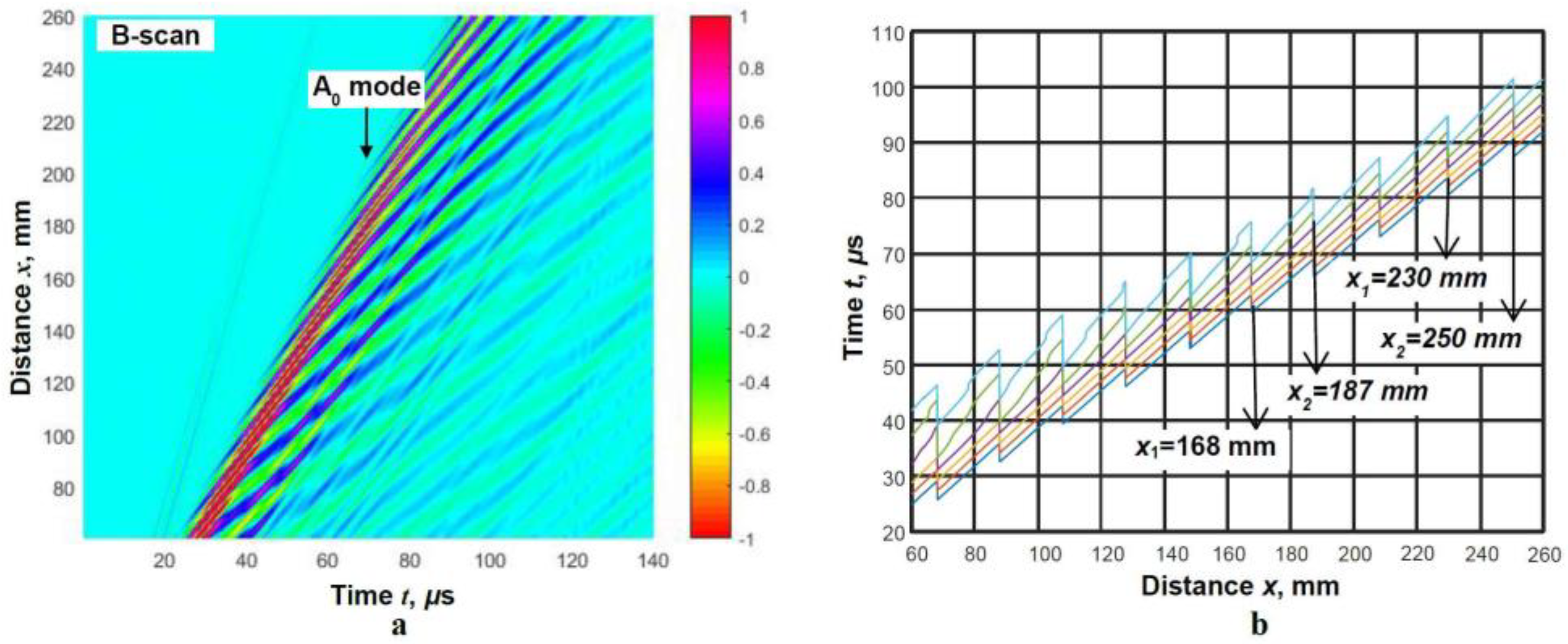
2.4.2. Evaluating Phase Velocity across Various Dispersion Ranges

Theoretical studies were carried out at three different frequency ranges: 150 kHz, 500 kHz and 900 kHz. These studies used simulated signals of the A₀ mode, as shown in the B-scan images (Figure 2a,c,d). For each scenario, the maximum distances between two signals where the time-of-flight can be measured between identical phase points should be calculated. Since, the maximum distance was calculated according to Equation (7), both the phase and group velocities at the central frequencies should be determined. Thus, in order to obtain the dispersion curves of the phase and group velocities, the elastic constants of the material and the object’s geometry must be known (Figure 1). Based on this, the maximum distance between two signals was determined according to Equation (7). The phase and group velocities determined in the analysed frequency ranges, along with the calculated maximum distances between two possible signals, are presented in

Table 3. The calculated values of the phase and group velocities at different central frequency of the A₀ mode of Lamb waves and maximal distance $∆l$ between two signals.

Frequency, kHz	Phase Velocity, m/s	Group Velocity, m/s	$\mathbf{Distance}∆\mathit{l},\mathbf{m}\mathbf{m}$
150	1547	2571	25
500	2323	3115	18
900	2625	3117	18

.

The phase velocity is calculated by applying the zero-crossing technique, setting the threshold level to U_L = 0.1 and determining six time instants at which the signal crosses the zero-amplitude line for each case. The measured zero-crossing instants at the different propagating distances are presented in Figure 6a–c. The obtained segments of the phase velocity using two signals in each frequency range alongside the dispersion curve calculated by the SAFE method are presented in Figure 6d.

The reconstructed segments of the phase velocity dispersion curve at different frequencies are compared with the dispersion curve calculated by the SAFE method, and the mean relative error is calculated in each case according to Equation (8). The obtained results are presented in

Table 4. The calculated results of the mean relative error ${\delta }_{c_{ph}}$ using pair of the signals at different frequencies.

Frequency, kHz	150	500	900
${\delta }_{cph}$, %	0.33	0.23	0.11

.

The obtained results of the theoretical study show that the segments of the phase velocity dispersion curves can be estimated across various frequency ranges using only two received signals. Therefore, the experimental study needed to be performed for the verification of the obtained theoretical results.

3. Experimental Study

An experimental study was carried out to verify the obtained theoretical results by reconstructing the phase velocity dispersion curves in a dispersive medium using only two signals. The A₀ mode of Lamb waves were selected for the study. The experimentally obtained signals of the Lamb waves propagating in an isotropic aluminium plate were used for the study. An aluminium plate, with dimensions of 1.1 m × 0.62 m and thickness of 2 mm, was chosen for the experimental study. The parameters of the aluminium alloy plate were the same as in the analytical verification: Young modulus E = 71.7 GPa, Poisson‘s ratio ν = 0.33 and density ρ = 2810 kg/m³. The experimental set-up for generating and receiving of the A₀ mode signals is presented in Figure 7.

The ultrasonic measurement system “Ultralab”, consisting of a voltage generator, a low-noise amplifier and an analogue-to-digital converter, was used for the excitation and reception of Lamb wave signals (Figure 7). Two low-frequency, wideband contact-type ultrasonic transducers with 180 kHz resonant frequency, whose frequency bandwidth was from 40 kHz up to 640 kHz (at −10 dB) [27], were used in the experimental study. The resonant frequency of the contact transducers was chosen to be the same as in the analytical study and was 300 kHz. The transmitter was excited by a three-period burst Gaussian envelope signal with an amplitude of 10 V and was mounted in the selected location on the plate. The position of the receiver was changed with a linear scanner. In order to investigate the possibility of reconstructing the phase velocity dispersion curves using only two signals acquired at different propagating distances, a set of experimentally collected signals was used. The receiver was scanned along the surface of the sample, from 60 mm up to 260 mm in 0.1 mm increments, and the B-scan image of the A₀ mode was acquired. The threshold level U_L = 0.1 was selected, and six-time instants at which the signals crossed the zero-amplitude line were selected. The experimentally collected signals of the Lamb wave A₀ mode are presented in the B-scan image (Figure 8a), and the measured zero-crossing instants of the propagation distance are shown in Figure 8b.

Two different distances were selected for the A₀ mode study. The first distance was from 168 mm up to 187 mm, and the second was from 230 mm up to 250 mm. The pairs of the signals at different distances between two points, x₁ = 168 mm and x₂ = 187 mm, and x₁ = 230 mm and x₂ = 250 mm, were selected for further study.

The reconstructed segments of the phase velocity dispersion curves of the A₀ mode using pair of the experimentally measured signals at different distances were compared with those calculated by the SAFE method and presented in Figure 9a,b, respectively. The mean relative error was calculated for the reconstructed segment of the phase velocity according to Equation (8), and the obtained results are presented in

Table 5. The calculated experimental results of the mean relative error ${\delta }_{c_{ph}}$ using a pair of signals at different analysed distances.

Distance of the signals, mm		x1 = 168; x2 = 187	x1 = 230; x2 = 250
A0 mode	${\delta }_{c_{ph}}$, %	0.91	1.36

.

The obtained experimental results show that the phase velocity dispersion curves can be reconstructed using only two signals, as shown in Figure 9a,b. An important condition is that the distance between two possible signals should be known. If this condition is met, then the segment of the phase velocity dispersion curve can be reconstructed at any distance of the wave propagation path. Based on the reconstructed segments of the phase velocity dispersion curve, the mean relative error ${\delta }_{c_{ph}}$ was calculated according to Equation (8) for both analysed cases. The mean relative error ${\delta }_{c_{ph}}=0.91\%$ was obtained at the distance x₁ = 168 mm and x₂ = 187, and ${\delta }_{c_{ph}}=1.36\%$ at the distance x₁ = 230 mm and x₂ = 250. So, the obtained experimental results confirmed the theoretical results. Therefore, this technique can be applied to solve various tasks, serving as a useful tool that allows for the saving of both time and effort.

4. Conclusions

The presented work analyses the possibility of reconstructing a segment of the phase velocity in the strong dispersion range using only two received signals. The basic parameters and regularities required for the reconstruction of the phase velocity dispersion curve using two received signals were presented and thoroughly explained. The theoretical and experimental studies were performed using signals of the anti-symmetric A₀ mode of Lamb waves propagating in an aluminium plate. The 300 kHz range was chosen for the study, where the A₀ mode had a strong dispersion character. It was determined that the maximum distance between two signals registration points at which the time-of-flight can be measured between the same phase points is the main parameter which should first be known. Thus, the elastic constants of the material and the geometry of the object need to be known in order to calculate the dispersion curves of the phase and group velocities, based on which the maximum distance between two possible signals is determined. This is the main limitation of the method. Therefore, this method, in its current form, can be used to analyse guided wave propagation in known objects.

A comparison of the theoretical and experimental results with the SAFE method was performed, and the mean relative error was calculated for each analysed case. In the theoretical study, the mean relative error obtained was 0.33%, 0.22%, 0.23% and 0.11% at 150 kHz, 300 kHz, 500 kHz and 900 kHz frequency ranges, accordingly. The obtained results indicate that the phase velocity evaluation in the dispersion range using only two received signals is a solvable task. The experimental study confirmed that the segments of the phase velocity dispersion curve can be reconstructed in the strong dispersion range using only two received signals. The calculated mean relative error ${\delta }_{c_{ph}}=0.91\%$ is obtained at the distance x₁ = 168 mm and x₂ = 187, and ${\delta }_{c_{ph}}=1.36\%$ at the distance x₁ = 230 mm and x₂ = 250. The application of this technique can be used to solve various tasks where phase velocity values are required. It serves as a practical tool, saving both time and effort.

References

1. Masserey, B.; Raemy, C.; Fromme, P. High-frequency guided ultrasonic waves for hidden defect detection in multi-layered aircraft structures. Ultrasonics 2014, 54, 1720–1728. [Google Scholar] [CrossRef] [PubMed] [Green Version]
2. Chia, C.C.; Lee, S.Y.; Harmin, M.Y.; Choi, Y.; Lee, J.-R. Guided ultrasonic waves propagation imaging: A review. Meas. Sci. Technol. 2023, 34, 052001. [Google Scholar] [CrossRef]
3. Yang, Z.; Yang, H.; Tian, T.; Deng, D.; Hu, M.; Ma, J.; Wu, Z. A review in guided-ultrasonic-wave-based structural health monitoring: From fundamental theory to machine learning techniques. Ultrasonics 2023, 133, 107014. [Google Scholar] [CrossRef]
4. Hu, Y.; Zhu, Y.; Tu, X.; Lu, J.; Li, F. Dispersion curve analysis method for Lamb wave mode separation. Struct. Health Monit. 2020, 19, 1590–1601. [Google Scholar] [CrossRef]
5. Pai, P.F.; Deng, H.; Sundaresan, M.J. Time-frequency characterization of lamb waves for material evaluation and damage inspection of plates. Mech. Syst. Signal Process. 2015, 62–63, 183–206. [Google Scholar] [CrossRef]
6. Gorgin, R.; Luo, Y.; Wu, Z. Environmental and operational conditions effects on Lamb wave based structural health monitoring systems: A review. Ultrasonics 2020, 105, 106114. [Google Scholar] [CrossRef]
7. Yang, T.; Zhou, W.; Yu, L. Guided Wave-Based Damage Detection of Square Steel Tubes Utilizing Structure Symmetry. Symmetry 2023, 15, 805. [Google Scholar] [CrossRef]
8. Xie, J.; Ding, W.; Zou, W.; Wang, T.; Yang, J. Defect Detection inside a Rail Head by Ultrasonic Guided Waves. Symmetry 2022, 14, 2566. [Google Scholar] [CrossRef]
9. Chen, H.; Zhang, G.; Fan, D.; Fang, L.; Huang, L. Nonlinear Lamb wave analysis for microdefect identification in mechanical structural health assessment. Measurement 2020, 164, 108026. [Google Scholar] [CrossRef]
10. Draudviliene, L.; Meskuotiene, A.; Mazeika, L.; Raisutis, R. Assessment of Quantitative and Qualitative Characteristics of Ultrasonic Guided Wave Phase Velocity Measurement Technique. J. Nondestr. Eval. 2017, 36, 22. [Google Scholar] [CrossRef]
11. Zima, B.; Woloszyk, K.; Garbatov, Y. Corrosion degradation monitoring of ship stiffened plates using guided wave phase velocity and constrained convex optimization method. Ocean. Eng. 2022, 253, 111318. [Google Scholar] [CrossRef]
12. Olisa, S.C.; Khan, M.A.; Starr, A. Review of Current Guided Wave Ultrasonic Testing (GWUT) Limitations and Future Directions. Sensors 2021, 21, 811. [Google Scholar] [CrossRef]
13. Jia, H.; Zhang, Z.; Liu, H.; Dai, F.; Liu, Y.; Leng, J. An approach based on expectation-maximization algorithm for parameter estimation of Lamb wave signals. Mech. Syst. Signal Process. 2019, 120, 341–355. [Google Scholar] [CrossRef]
14. Wilcox, P.D. A rapid signal processing technique to remove the effect of dispersion from guided wave signals. IEEE Trans. Ultrason. Ferroelectr. Freq. Control. 2003, 50, 419–427. [Google Scholar] [CrossRef] [PubMed]
15. Su, Z.; Ye, L.; Lu, Y. Guided Lamb waves for identification of damage in composite structures: A review. J. Sound Vib. 2006, 295, 753–780. [Google Scholar] [CrossRef]
16. Dai, D.; He, Q. Structure damage localization with ultrasonic guided waves based on a time–frequency method. Signal Process. 2014, 96, 21–28. [Google Scholar] [CrossRef]
17. Golub, M.V.; Doroshenko, O.V.; Arsenov, M.A.; Bareiko, I.A.; Eremin, A.A. Identification of Material Properties of Elastic Plate Using Guided Waves Based on the Matrix Pencil Method and Laser Doppler Vibrometry. Symmetry 2022, 14, 1077. [Google Scholar] [CrossRef]
18. Ghose, B.; Panda, R.S.; Balasubramaniam, K. Phase velocity measurement of dispersive wave modes by Gaussian peak-tracing in the f-k transform domain. Meas. Sci. Technol. 2021, 32, 124006. [Google Scholar] [CrossRef]
19. Zeng, L.; Huang, L.; Cao, X.; Gao, F. Determination of Lamb wave phase velocity dispersion using time–frequency analysis. Smart Mater. Struct. 2019, 28, 115029. [Google Scholar] [CrossRef]
20. Zeng, L.; Cao, X.; Huang, L.; Luo, Z. The measurement of Lamb wave phase velocity using analytic cross-correlation method. Mech. Syst. Signal Process 2021, 151, 107387. [Google Scholar] [CrossRef]
21. Crespo, B.H.; Courtney, C.; Engineer, B. Calculation of Guided Wave Dispersion Characteristics Using a Three-Transducer Measurement System. Appl. Sci. 2018, 8, 1253. [Google Scholar] [CrossRef] [Green Version]
22. Draudviliene, L.; Tumsys, O.; Mazeika, L.; Zukauskas, E. Estimation of the Lamb wave phase velocity dispersion curves using only two adjacent signals. Compos. Struct. 2021, 258, 113174. [Google Scholar] [CrossRef]
23. Zima, B.; Woloszyk, K.; Garbatov, Y. Experimental and numerical identification of corrosion degradation of ageing structural components. Ocean Eng. 2022, 258, 111739. [Google Scholar] [CrossRef]
24. Bartoli, I.; Marzani, A.; di Scalea, F.L.; Viola, E. Modeling wave propagation in damped waveguides of arbitrary cross-section. J. Sound Vib. 2006, 295, 685–707. [Google Scholar] [CrossRef]
25. Hayashi, T.; Song, W.-J.; Rose, J.L. Guided wave dispersion curves for a bar with an arbitrary cross-section, a rod and rail example. Ultrasonics 2003, 41, 175–183. [Google Scholar] [CrossRef]
26. He, P. Simulation of ultrasound pulse propagation in lossy media obeying a frequency power law. IEEE Trans. Ultrason. Ferroelectr. Freq. Control. 1998, 45, 114–125. [Google Scholar] [CrossRef] [Green Version]
27. Vladišauskas, A.; Šliteris, R.; Raišutis, R.; Seniūnas, G.; Žukauskas, E. Contact ultrasonic transducers for mechanical scanning systems. Ultragarsas 2010, 65, 30–35. [Google Scholar]
Figure 1. The phase and group velocity dispersion curves of the A0 mode of Lamb waves calculated using the SAFE method.
Symmetry 15 01236 g001
Figure 2. The B-scan images of the simulated A0 mode of Lamb waves at 150 kHz, 300 kHz, 500 kHz and 900 kHz (ad), accordingly.
Symmetry 15 01236 g002
Figure 3. The A0 mode signal at a distance of 100 mm (a) and measured zero-crossing instants versus distance (b), the A0 mode signal at a distance of 139 mm (c), 158 mm (d) and 160 mm (e).
Symmetry 15 01236 g003
Figure 4. Measured zero-crossing instants at the whole propagating distance of the A0 mode (a) and the zero-crossing instants at the analysed distance from 135 mm up to 160 mm (b). The different line colours represent the different time instants at which the signals cross the zero-amplitude line.
Symmetry 15 01236 g004
Figure 5. Measured zero-crossing instants at the propagating different distances: from 24 mm up to 43 mm (a), 120 mm up to 139 mm (b) and 177 mm up to 196 mm (c). The different line colours represent the different time instants at which the signals cross the zero-amplitude line. The obtained segments of the phase velocity, using two signals at different analysing distances, were plotted together with those calculated using the SAFE method (df), accordingly.
Symmetry 15 01236 g005
Figure 6. Measured zero-crossing instants at the different frequency ranges: 150 kHz (a), 500 kHz (b), 900 kHz (c) and the obtained segments of the phase velocity using two signals in each frequency case (d). The different line colours represent the different time instants at which the signals cross the zero-amplitude line.
Symmetry 15 01236 g006
Figure 7. The experimental set-up for generation and reception of Lamb waves in the aluminium plate.
Symmetry 15 01236 g007
Figure 8. The experimental B-scan image obtained for the A0 mode along the centreline of 2 mm thick aluminium plate (a) and measured zero-crossing instants along the propagating distance (b). The different line colours represent the different time instants at which the signals cross the zero-amplitude line.
Symmetry 15 01236 g008
Figure 9. The obtained segments of the phase velocity using two signals at the selected propagation distances: 168 mm–187 mm (a) and 230 mm–250 mm (b) are plotted together with those calculated via the SAFE method.
Symmetry 15 01236 g009