Numerical Approach for Solving a Fractional-Order Norovirus Epidemic Model with Vaccination and Asymptomatic Carriers

Abstract

This paper explored the impact of population symmetry on the spread and control of a norovirus epidemic. The study proposed a mathematical model for the norovirus epidemic that takes into account asymptomatic infected individuals and vaccination effects using a non-singular fractional operator of Atanganaa–Baleanu Caputo (ABC). Fixed point theory, specifically Schauder and Banach’s fixed point theory, was used to investigate the existence and uniqueness of solutions for the proposed model. The study employed MATLAB software to generate simulation results and demonstrate the effectiveness of the fractional order q. A general numerical algorithm based on Adams–Bashforth and Newton’s Polynomial method was developed to approximate the solution. Furthermore, the stability of the proposed model was analyzed using Ulam–Hyers stability techniques. The basic reproductive number was calculated with the help of next-generation matrix techniques. The sensitivity analysis of the model parameters was performed to test which parameter is the most sensitive for the epidemic. The values of the parameters were estimated with the help of least square curve fitting tools. The results of the study provide valuable insights into the behavior of the proposed model and demonstrate the potential applications of fractional calculus in solving complex problems related to disease transmission.

1. Introduction

The most dangerous infectious diseases were listed by medical sciences researchers through testing by various laboratories. Among them, one of the diseases of the stomach is caused by noroviruses (NoV), which enter through fecal–oral paths and interact with human feeding. These types of viruses may also be found in the shedding of vomitus. Besides these sources, the contamination of used food or water and contact with fomites or direct contact with any infected individuals may also cause this type of epidemic [1]. The local significance for each of these paths has been discussed but it is widely known that the NoV group of viruses alone is responsible for a huge epidemic due to food consumption and creates a burden on health in various countries [2,3]. The acute viral gastroenteritis viruses are related to three types of foods, which can cause an epidemic:

A₁:

The shells of molluscs are contaminated with different impurities during production.

A₂:

Fresh food items can be contaminated at the time of packing, collection, and harvesting.

A₃:

Taking more time to prepare and cook food can lead to contamination.

Poor practical and personal hygiene when handling foods is the main cause of contaminated food, which can lead to the transmission of an NoV epidemic. This type of food contamination will depend on many factors such as personal hygiene habits, the output of the virus, time of virus transfer, duration of the existence of the virus, time of inactivation for the virus, the shedding effect of the virus and many other factors. The contamination of hands may contaminate different surfaces depending upon the degree of touching and contamination of hands. The hands in this situation may contribute to the epidemic as well as receiving the disease [4]. The spreading of norovirus (NoV) and its results may depend on many factors. It may also depend on weather conditions and nearly half of the cases may occur in the winter season [5].

Mathematical models of epidemiological problems have been applied to the prediction and control of infectious diseases [6,7,8,9,10]. Different global problems of epidemic diseases have very interesting outcomes as represented by mathematical formulations given in the past literature. Some aspects of this concept include stochastic representation which have impacts, such as global humidity, perceptions, heat occurrence, etc., which affect the strength of the immune system against infective diseases. This idea will enable us to write the deterministic idea in the form of random situations which have more realistic outcomes. This will include all the other external impacts in the form of mathematical formulation. This will cause vibration in the parameters from the environment or some variation in the infectious models or due to the given system [11,12]. This approach of modeling provides more choices for selection and gives more realistic results as compared to the idealistic approach of deterministic models. Therefore, the stochastic concepts that are perturbed by white noise or Brownian motion are well represented in the literature, for detail one can see [13].

The relationship between symmetry and epidemic models relates to how the distribution of susceptible, infected, and recovered individuals in a population are affected by factors such as demographic and environmental symmetry. Symmetry considerations can play a role in the modeling of disease transmission dynamics, as they can affect the spatial and temporal spread of an epidemic. For example, if a population is asymmetric with respect to some underlying factor, such as age or location, this could lead to differences in the transmission of a disease and impact the effectiveness of control strategies. In the context of mathematical modeling, accounting for symmetry in the population being modeled can help to improve the accuracy of epidemic models and provide valuable insights into the spread and control of infectious diseases [14,15,16]. Fractional calculus, as used in the paper abstract mentioned earlier, is one approach to modeling the impact of symmetry in disease transmission dynamics. By developing models that account for the effects of asymmetry, researchers can gain a better understanding of the underlying mechanisms driving epidemics and develop more effective strategies to prevent and control their spread.

As we describe any system having different choices for the selection of the order of the derivative, the extra degrees will be obtained in the complex dynamics. This extra variety of choices can be studied in modern calculus in the form of non-natural order derivative expressions whose outcomes must be obtained as the whole density of the quantities [17,18,19]. Due to this, modern calculus will be superior to classical calculus. The medical sciences and natural sciences dynamical systems require more and more information, therefore these can be well investigated using different fractional operators for the internal behavior of the system; for the last few decades, this has been the central focus of many researchers as compared to the integer order analysis. In this field, the investigation is related to unique and solution existence, positivity, boundedness, numerical solution, and the realistic approach of feasibility. To date, various problems of small micro species, logistic population problems, HBV, TB, HCV, SIR, SEIR, SI, and many cancer problems have been investigated in the sense of fractional order derivatives [20,21,22,23,24]. These problems are tested for theoretical and approximate solutions in the non-integer order parameters sensed by the application of various techniques. Some examples are the Adams–Bashforth, corrector-predictor method, various transformations, and series solution techniques [25,26]. The analysis of COVID-19 problems has been investigated recently through fractional operators as can be seen in [27,28,29]. The literature is full of articles related to infectious disease problems and their analysis for different dynamics [30,31].

A fractional derivative is a generalization of the standard derivative to non-integer orders. It is defined using the Riemann–Liouville fractional integral, which is a generalization of the standard integral to non-integer orders [17,18]. The fractional derivative has applications in many areas of science and engineering, including mathematical biology. In mathematical biology, fractional derivatives are used to model various phenomena such as diffusion in porous media, blood flow in vessels, and the spread of diseases. For example, in the study of tumor growth, a fractional derivative model can be used to describe the diffusion of nutrients and oxygen through the tumor tissue, which is a non-local process. Additionally, in the study of the spread of infectious diseases, a fractional derivative model can be used to describe the spread of the disease through a population, which is also a non-local process. There have been a variety of fractional operators proposed in the literature with both nonsingular and singular kernels [20,21,22,23,24,32]. The work of [25,26,33,34,35] and references cited therein present a comprehensive study and the application of these fractional order operators as well as a detailed analysis of their implementation.

The Atangana–Baleanu fractional derivative is a particular type of fractional derivative that is defined using a Caputo–Fabrizio type of kernel function. It is named after its inventors, Atangana and Baleanu, who introduced it in their 2016 paper [25]. This fractional derivative is a generalization of the Caputo fractional derivative, which is one of the most widely used fractional derivatives in mathematical biology. It can be used to model various phenomena such as diffusion in porous media, blood flow in vessels, and the spread of diseases. In mathematical biology, the Atangana-Baleanu fractional derivative has been used to model various phenomena such as the spread of infectious diseases, tumor growth, and the spread of pollutants in a porous medium. For example, in the study of the spread of infectious diseases, a fractional derivative model can be used to describe the spread of the disease through a population, which is a non-local process. Additionally, in the study of tumor growth, the Atangana–Baleanu fractional derivative can be used to describe the diffusion of nutrients and oxygen through the tumor tissue, which is also a non-local process. In the study of the spread of pollutants in a porous medium, the Atangana–Baleanu fractional derivative can be used to describe the diffusion of pollutants through the porous medium, which is also a non-local process. It has been found that in many cases that the Atangana–Baleanu fractional derivative provides a better fit than other types of fractional derivatives, such as the Caputo fractional derivative, for the above-mentioned phenomena.

As for the motivation of our work, we kept in mind the above significance of fractional calculus and took a novel problem related to the norovirus (NoV) using the Atangana–Baleanu arbitrary order differentiation by applying the conditions of asymptomatic and vaccinated classes. For the discussion, different aspects of NoV mathematical formulation have been used. Here, we discuss the said epidemic with the inclusion of two classes of asymptomatic carriers and vaccinated classes for more effective analysis. There is a duration of 30–180 days in which the signs of NoV virus and the risk of infection by an infectious person with a chance of death can manifest [36,37]. On reviewing the literature, we have formulated a new problem for the NoV viruses with two new compartments [9,12,30,31]. Firstly, the problem was constructed for the integer order and, after that, it was modified and extended to the fractional version of the Atangana–Baleanu derivative. The main objective of this article was to evaluate the mathematical formulation, testing the problem on public health with vaccination and dilation of time for controlling an NoV epidemic.

The novelty of this paper is in the extension of the deterministic stochastic model [38] to the Atanga–Beleanu fractional model, which offers a more realistic approach to epidemic modeling. The ABC fractional operator model provides several advantages over stochastic models in the context of epidemic modeling. First of all, it provides a deterministic framework that makes it possible to precisely and deterministically analyze the dynamics of epidemics, especially when examining how population symmetry affects spread and control. Contrarily, stochastic models introduce randomness and variability, creating uncertainties and making it difficult to comprehend the effects of population symmetry. Second, for better comprehension and management of epidemics, the ABC fractional operator model incorporates critical elements such as asymptomatic infected individuals and vaccination effects. This thorough representation takes into account the sizeable portion of infected people who might not show any symptoms. Stochastic models have limitations in accurately determining the effectiveness of control strategies and interventions because they do not explicitly take into account asymptomatic individuals or vaccination effects. Furthermore, the ABC model benefits from the application of fixed point theory, such as Schauder and Banach’s fixed point theory, to analyze the existence and uniqueness of solutions. This mathematical approach provides rigorous foundations, ensuring reliable and valid outcomes. In contrast, stochastic models heavily rely on probabilistic methods and simulations, which can be computationally intensive and susceptible to statistical fluctuations. Moreover, the utilization of MATLAB software in the ABC model enables efficient computation and visualization of epidemic dynamics. This capability facilitates insights into model behavior under various scenarios and interventions, supporting informed decision-making in epidemic control. Collectively, the advantages of the ABC fractional operator model make it a valuable tool for epidemic modeling, offering greater realism and enhanced analytical capabilities compared to stochastic models.

The organization of this paper is as follows: Ii Section 2, we will formulate a novel mathematical model. Section 3 presents some basic definitions of fractional operators. In Section 4, the mathematical analysis determines whether there is a solution that exists and how certain terms can be optimized (3). The qualitative theory is studied in Section 5. The basic reproductive number and sensitivity analysis of the model are presented in Section 6. Section 7 studied the approximate solution of the model (3). Section 8 presented the parameter estimation of the model. In Section 9, we verify our theoretical results using numerical simulations. At the end of this paper, we summarize the main findings of our research in a section titled Conclusions.

2. Model Formulation

We extended Cui et al.’s model [38] which has five equations that are applicable to the considered infection mathematical model describing norovirus (NoV). All the density of individuals is distributed in five different compartmental agents, namely: Susceptible class $\left(\mathcal{H}\right)$, Vaccinated individuals $\left(\mathcal{V}\right)$, Asymptomatic or Exposed individuals $\left(\mathcal{U}\right)$, Symptomatic or Infectious individuals $\left(\mathcal{A}\right)$, and the Recovered class $\left(\mathcal{C}\right)$, i.e., $H\left(t\right)+V\left(t\right)+U\left(t\right)+A\left(t\right)+C\left(t\right))=N(t)$. The equations describing the model are

$$\begin{array}{cc}\hfill \acute{\mathcal{H}}& =\mathsf{\Lambda }-\frac{\eta \mathcal{H}\left(t\right)\mathcal{A}\left(t\right)}{N}-\mathcal{H}\left(t\right)(\rho +d),\hfill \\ \hfill \acute{\mathcal{V}}& =\rho \mathcal{H}\left(t\right)-\frac{(1-\tau )\eta \mathcal{A}\left(t\right)}{N}-d\mathcal{V}\left(t\right),\hfill \\ \hfill \acute{\mathcal{U}}& =\frac{\eta \mathcal{H}\left(t\right)\mathcal{A}\left(t\right)}{N}+\frac{(1-\tau )\eta \mathcal{V}\left(t\right)\mathcal{A}\left(t\right)}{N}-(\alpha +d)\mathcal{U}\left(t\right),\hfill \\ \hfill \acute{\mathcal{A}}& =\alpha \mathcal{U}\left(t\right)-(q+d)\mathcal{A}\left(t\right),\hfill \\ \hfill \acute{\mathcal{C}}& =\delta \mathcal{A}\left(t\right)-d\mathcal{C}\left(t\right),\hfill \end{array}$$

(1)

with the starting approximation,

$$H\left(0\right)\ge 0,V\left(0\right)\ge 0,A\left(0\right)\ge 0,U\left(0\right)\ge 0,R\left(0\right)\ge 0,$$

(2)

where $\mathsf{\Lambda }$ is the recruitment rate representing the rate at which individuals enter the susceptible population. $\eta$ is the transmission rate representing the probability of transmission per contact between susceptible individuals and infected individuals. $\mathcal{H}\left(t\right)$ represents the density of individuals in the susceptible (healthy) class at time t. The rate of change of $\mathcal{H}\left(t\right)$ is determined by the balance between recruitment ($\mathsf{\Lambda }$), transmission $\frac{\eta \mathcal{H}\left(t\right)\mathcal{A}\left(t\right)}{N}$, and the natural removal $\mathcal{H}\left(t\right)(\rho +d)$ of individuals. $\mathcal{V}\left(t\right)$ represents the density of vaccinated individuals at time t. The balance between transmission from susceptible individuals $\rho \mathcal{H}\left(t\right)$, transmission from immunized individuals $\frac{\left[\right(1-\tau \left)\eta \mathcal{A}\right(t\left)\right]}{N}$, and natural removal of individuals $d\mathcal{V}\left(t\right)$ determines the rate of change of $\mathcal{V}\left(t\right)$. The density of people who are asymptomatic or exposed at time t is represented by $\mathcal{U}\left(t\right)$. The balance between transmission from susceptible individuals and $\mathcal{U}\left(t\right)$ determines the rate of change of this variable. $\frac{\eta \mathcal{H}\left(t\right)\mathcal{A}\left(t\right)}{N}$, transmission from immunized people $\frac{\left[\right(1-\tau \left)\eta \mathcal{V}\right(t\left)\mathcal{A}\right(t)}{N}$, recovery of people $(\alpha +d)\mathcal{U}\left(t\right)$, and natural removal. $\mathcal{A}\left(t\right)$ indicates the proportion of people who are symptomatic or contagious at time t. The balance between natural removal, $\frac{\left[\right(q+d\left)\mathcal{A}\right(t\left)\right]}{N}$, and transmission to susceptible individuals $\alpha \mathcal{U}\left(t\right)$ determines the rate of change of $\mathcal{A}\left(t\right)$. $\mathcal{C}\left(t\right)$ represents the density of people who have been found at time t. The recovery of individuals $\delta \mathcal{A}\left(t\right)$ and natural removal $d\mathcal{C}\left(t\right)$ determine the rate of change of $\mathcal{C}\left(t\right)$. The system of equations captures the interactions between those who are susceptible, those who have received vaccinations, those who are asymptomatic, those who are symptomatic, and those who have recovered to describe the dynamics of the norovirus epidemic. The spread and management of the epidemic over time are influenced by the rates of transmission, recovery, and removal as well as the population size N. The behavior’s transition points are shown in Figure 1.

The key objective was to construct a new numerical system (1) using the ABC fractional derivative for an extra degree of choices of dynamical behavior. The qualitative analysis will be derived by the application of fixed point theory. The considered numerical problem will be analyzed, having a general derivative order of $\eta$ as follows:

$$\left\{\begin{array}{cc}\hfill {}^{ABC}{D}^q\mathcal{H}\left(t\right)& =\mathsf{\Lambda }-\frac{\eta \mathcal{H}\left(t\right)\mathcal{A}\left(t\right)}{N}-(\rho +d)\mathcal{H}\left(t\right),\hfill \\ \hfill {}^{ABC}{D}^q\mathcal{V}\left(t\right)& =\rho \mathcal{H}\left(t\right)-\frac{(1-\tau )\eta \mathcal{A}\left(t\right)}{N}-d\mathcal{V}\left(t\right),\hfill \\ \hfill {}^{ABC}{D}^q\mathcal{U}\left(t\right)& =\frac{\eta \mathcal{H}\left(t\right)\mathcal{A}\left(t\right)}{N}+\frac{(1-\tau )\eta \mathcal{V}\left(t\right)\mathcal{A}\left(t\right)}{N}-(\alpha +d)\mathcal{U}\left(t\right),\hfill \\ \hfill {}^{ABC}{D}^q\mathcal{A}\left(t\right)& =\alpha \mathcal{U}\left(t\right)-(q+d)\mathcal{A}\left(t\right),\hfill \\ \hfill {}^{ABC}{D}^q\mathcal{C}\left(t\right)& =\delta \mathcal{A}\left(t\right)-d\mathcal{C}\left(t\right).\hfill \end{array}\right.$$

(3)

3. Preliminaries

This section introduces the $\mathcal{ABC}$ operator and its properties, along with the numerical approximation method for solving fractional order differential equations.

Definition 1.

If $\mathsf{\Pi }\left(t\right)\in {\mathfrak{G}}^1(0,\mathcal{T})$ and $q\in (0,1]$, then $\mathcal{ABC}$ is formulated as

$${}^{ABC}{D}_{+0}^q\mathsf{\Pi }\left(t\right)=\frac{M\left(q\right)}{1-q}{\int }_0^t\frac{d}{dx}\mathsf{\Pi }\left(y\right)M_q\left[\frac{-q}{1-q}(t-y)\right]dy,$$

(4)

replacing $M_q\left[\frac{-q}{1-q}(t-y)\right]dy$ by $M_1=exp\left[\frac{-q}{1-q}(t-y)\right]$, we obtain the Caputo–Fabrizo fractional derivative. It should be noticed that

$${}^{ABC}{D}_{+0}^q\left[Constant\right]=0;$$

here, $M\left(q\right)$ is named the normal mapping given as $M\left(0\right)=M\left(1\right)=1$. $M_q$ represents Mittag–Leffler mapping, the generalized exponent mapping [39,40,41].

In Definition 1, the $\mathcal{ABC}$ operator is defined as a fractional derivative operator, denoted by ${}^{ABC}{D}_{+0}^q$, where $\mathsf{\Pi }\left(t\right)$ is a function belonging to the space ${\mathfrak{G}}^1(0,\mathcal{T})$ and q is a parameter in the range $(0,1]$. The operator is expressed as an integral involving the derivative of $\mathsf{\Pi }$ and a Mittag–Leffler mapping $M_q$, with $M_1$ representing the exponential function. The lemma also states the behavior of the operator for constant values.

Lemma 1.

[42] Solution of the given equation for $1>q>0$,

$$\begin{array}{cc}& {}^{ABC}{D}_{+0}^q\mathfrak{Z}\left(t\right)=x\left(t\right),t\in [0,T],\hfill \\ & \mathfrak{Z}\left(0\right)={\mathfrak{Z}}_0,\hfill \end{array}$$

(5)

is given by

$$\mathfrak{Z}\left(t\right)={\mathfrak{Z}}_0+\frac{(1-q)}{M\left(q\right)}x\left(t\right)+\frac{q}{\mathsf{\Gamma }\left(q\right)M\left(q\right)}{\int }_0^t{(t-y)}^{q-1}x\left(y\right)dy.$$

Lemma 1 provides the solution to a fractional differential equation in terms of the $\mathcal{ABC}$ operator. The equation ${}^{ABC}{D}_{+0}^q\mathfrak{Z}\left(t\right)=x\left(t\right)$ represents a fractional order differential equation, where $\mathfrak{Z}\left(t\right)$ is the unknown function and $x\left(t\right)$ is a given function. The lemma presents the explicit solution $\mathfrak{Z}\left(t\right)$ in terms of the initial condition ${\mathfrak{Z}}_0$, the function $x\left(t\right)$, and the parameters q, $M\left(q\right)$, and $\mathsf{\Gamma }\left(q\right)$.

Definition 2.

We can convert the fractional order DEs with order q in the form of the ABC derivative as

$$\begin{array}{cc}\hfill {}^{ABC}{D}^q\mathcal{Y}\left(t\right)& =f(t,\mathcal{Y}(t\left)\right)\hfill \\ \hfill \mathcal{Y}\left(0\right)& ={\mathcal{Y}}_0.\hfill \end{array}$$

(6)

Then, the approximate solution of (6) is given as follows:

$$\begin{array}{cc}\hfill \mathcal{Y}\left(t_{m+1}\right)& ={\mathcal{Y}}_0+\frac{1-q}{M\left(q\right)}f(t_m,\mathcal{Y}\left(t_m\right))\hfill \\ \hfill & +\frac{q}{\mathsf{\Gamma }\left(q\right)M\left(q\right)}\sum _{k=0}^m(\frac{h^{q}f(t_k,{\mathcal{Y}}_k)}{\mathsf{\Gamma }(q+2)}\left({(1+m-k)}^q(-k+m+2+q)\right.\hfill \\ \hfill & \left.-{(-k+m)}^q(-k+m+2+2q)\right)\hfill \\ \hfill & -\frac{h^{q}f(t_{k-1},{\mathcal{Y}}_{k-1})}{\mathsf{\Gamma }(q+2)}\left({(1+m-k)}^{q+1}-{(-k+m)}^q(-k+m+1+q)\right)).\hfill \end{array}$$

(7)

Definition 2 introduces the conversion of fractional order differential equations to the ABC derivative form. The equation ${}^{ABC}{D}^q\mathcal{Y}\left(t\right)=f(t,\mathcal{Y}\left(t\right))$ represents a fractional order differential equation with the unknown function $\mathcal{Y}\left(t\right)$ and the function $f(t,\mathcal{Y}(t\left)\right)$ on the right-hand side. The definition provides an approximation method for solving such equations using the $\mathcal{ABC}$ operator. The approximate solution $\mathcal{Y}\left(t_{m+1}\right)$ is expressed recursively in terms of the initial condition ${\mathcal{Y}}_0$, the function $f(t,\mathcal{Y}(t\left)\right)$, and parameters q, $M\left(q\right)$, $\mathsf{\Gamma }\left(q\right)$, and h.

4. The Theory of Existence of Solution

The existence of the solutions for the given fractional order model is presented in this part of the paper; for this purpose, we try to define a function as follows:

$$\left\{\begin{array}{cc}\hfill {\mathsf{\Pi }}_1\left(t,\mathcal{H},\mathcal{V},\mathcal{U},\mathcal{A},\mathcal{C}\right)& =\mathsf{\Lambda }-\frac{\eta \mathcal{H}\left(t\right)\mathcal{A}\left(t\right)}{N}-\mathcal{H}\left(t\right)(\rho +d),\hfill \\ \hfill {\mathsf{\Pi }}_2\left(t,\mathcal{H},\mathcal{V},\mathcal{U},\mathcal{A},\mathcal{C}\right)& =\rho \mathcal{H}\left(t\right)-\frac{(1-\tau )\eta \mathcal{A}\left(t\right)}{N}-d\mathcal{V}\left(t\right),\hfill \\ \hfill {\mathsf{\Pi }}_3\left(t,\mathcal{H},\mathcal{V},\mathcal{U},\mathcal{A},\mathcal{C}\right)& =\frac{\eta \mathcal{H}\left(t\right)\mathcal{A}\left(t\right)}{N}+\frac{(1-\tau )\eta \mathcal{V}\left(t\right)\mathcal{A}\left(t\right)}{N}-\mathcal{U}\left(t\right)(\alpha +d),\hfill \\ \hfill {\mathsf{\Pi }}_4\left(t,\mathcal{H},\mathcal{V},\mathcal{U},\mathcal{A},\mathcal{C}\right)& =\alpha \mathcal{U}\left(t\right)-(q+d)\mathcal{A}\left(t\right),\hfill \\ \hfill {\mathsf{\Pi }}_5\left(t,\mathcal{H},\mathcal{V},\mathcal{U},\mathcal{A},\mathcal{C}\right)& =\delta \mathcal{A}\left(t\right)-d\mathcal{C}\left(t\right).\hfill \end{array}\right.$$

(8)

Using (8), the model is expressed as follows:

$$\begin{array}{cc}& {}^{ABC}{D}_{+0}^q\mathfrak{Z}\left(t\right)=\mathsf{\Pi }(t,\mathfrak{Z}\left(t\right)),t\in [0,T],0<q\le 1,\hfill \\ & \mathfrak{Z}\left(0\right)={\mathfrak{Z}}_0.\hfill \end{array}$$

(9)

Using Lemma (1), Equation (9) becomes

$$\mathfrak{Z}\left(t\right)={\mathfrak{Z}}_0\left(t\right)+\left[\mathsf{\Pi }\right((t,\mathfrak{Z}\left(t\right))-{\mathsf{\Pi }}_0\left(t\right)]\frac{1-q}{M\left(q\right)}+\frac{q}{M\left(q\right)\mathsf{\Gamma }\left(q\right)}{\int }_0^t{(t-y)}^{q-1}\mathsf{\Pi }(y,\mathfrak{Z}\left(y\right))dy,for0\le y\le t\le 1,$$

(10)

where

$$\mathfrak{Z}\left(t\right)=\left\{\begin{array}{cc}& \mathcal{H}\left(t\right)\hfill \\ & \mathcal{V}\left(t\right)\hfill \\ & \mathcal{U}\left(t\right)\hfill \\ & \mathcal{A}\left(t\right)\hfill \\ & \mathcal{C}R\left(t\right)\hfill \end{array}\right.,{\mathfrak{Z}}_0\left(t\right)=\left\{\begin{array}{cc}& {\mathcal{H}}_0\hfill \\ & {\mathcal{V}}_0\hfill \\ & {\mathcal{U}}_0\hfill \\ & {\mathcal{A}}_0\hfill \\ & {\mathcal{C}}_0\hfill \end{array}\right.,\mathsf{\Pi }(t,\mathfrak{Z}\left(t\right))=\left\{\begin{array}{cc}& {\mathsf{\Pi }}_1(t,\mathcal{H},\mathcal{V},\mathcal{U},\mathcal{A},\mathcal{C})\hfill \\ & {\mathsf{\Pi }}_2(t,\mathcal{H},\mathcal{V},\mathcal{U},\mathcal{A},\mathcal{C})\hfill \\ & {\mathsf{\Pi }}_3(t,\mathcal{H},\mathcal{V},\mathcal{U},\mathcal{A},\mathcal{C})\hfill \\ & {\mathsf{\Pi }}_4(t,\mathcal{H},\mathcal{V},\mathcal{U},\mathcal{A},\mathcal{C})\hfill \\ & {\mathsf{\Pi }}_5(t,\mathcal{H},\mathcal{V},\mathcal{U},\mathcal{A},\mathcal{C})\hfill \end{array}\right.,{\mathsf{\Pi }}_0\left(t\right)\left\{\begin{array}{cc}& {\mathsf{\Pi }}_1(0,{\mathcal{H}}_0,{\mathcal{V}}_0,{\mathcal{U}}_0,{\mathcal{A}}_0,{\mathcal{C}}_0)\hfill \\ & {\mathsf{\Pi }}_2(0,{\mathcal{H}}_0,{\mathcal{V}}_0,{\mathcal{U}}_0,{\mathcal{A}}_0,{\mathcal{C}}_0)\hfill \\ & {\mathsf{\Pi }}_3(0,{\mathcal{H}}_0,{\mathcal{V}}_0,{\mathcal{U}}_0,{\mathcal{A}}_0,{\mathcal{C}}_0)\hfill \\ & {\mathsf{\Pi }}_4(0,{\mathcal{H}}_0,{\mathcal{V}}_0,{\mathcal{U}}_0,{\mathcal{A}}_0,{\mathcal{C}}_0)\hfill \\ & {\mathsf{\Pi }}_5(0,{\mathcal{H}}_0,{\mathcal{V}}_0,{\mathcal{U}}_0,{\mathcal{A}}_0,{\mathcal{C}}_0)\hfill \end{array}\right.$$

(11)

Using (10) and (11), define two operators $\mathcal{F}$ and $\mathcal{G}$, using (10)

$$\begin{array}{cc}& \mathcal{F}\mathfrak{Z}={\mathfrak{Z}}_0\left(t\right)+[\mathsf{\Pi }(t,\mathfrak{Z}\left(t\right))-{\mathsf{\Pi }}_0\left(t\right)]\frac{1-q}{M\left(q\right)},\hfill \\ & \mathcal{G}\mathfrak{Z}=\frac{q}{M\left(q\right)\mathsf{\Gamma }\left(q\right)}{\int }_0^t{(t-y)}^{q-1}\mathsf{\Pi }(y,\mathfrak{Z}\left(y\right))dy.\hfill \end{array}$$

(12)

Furthermore, we reassume that the conditions ${\mathbf{D}}_1$ and ${\mathbf{D}}_2$ holds

$\left({\mathbf{D}}_{\mathbf{1}}\right)$ If fixed ${\sigma }_1$ and ${\sigma }_2$, as

$$\left|\mathsf{\Pi }(t,\mathfrak{Z}\left(t\right))\right|\le {\sigma }_1\left|\mathfrak{Z}\left(t\right)\right|+{\sigma }_2.$$

$\left({\mathbf{D}}_{\mathbf{2}}\right)$ If fixed $\kappa >0$, for all $\mathfrak{Z},{\mathfrak{Z}}_1\in \mathbb{X}$, as

$$|\mathsf{\Pi }(t,\mathfrak{Z}\left(t\right))-\mathsf{\Pi }(t,{\mathfrak{Z}}_1\left(t\right))|\le \kappa ||\mathfrak{Z}-{\mathfrak{Z}}_1\left|\right|.$$

Theorem 1.

If $\left({\mathbf{D}}_{\mathbf{1}}\right)$ and $\left({\mathbf{D}}_{\mathbf{2}}\right)$ are fulfilled, then system (10) will have at least a unique root, implying that our problem (3) has at least one root if

$$\frac{(1-q)\kappa }{M\left(q\right)}<1.$$

Proof. 

For the derivation of $\mathcal{F}$ to be a contraction operator, let ${\mathfrak{Z}}_1\in \mathbb{B}$, while $\mathbb{B}=\{\mathfrak{Z}\in \mathbb{Y}:|\left|\mathfrak{Z}\right||\le r,r>0\}$ is a closed convex set. Applying the result of $\mathcal{F}$ from (12), as

$$\begin{array}{cc}& \left|\right|\mathcal{F}\mathfrak{Z}-\mathcal{F}{\mathfrak{Z}}_1\left|\right|=\frac{(1-q)}{M\left(q\right)}\underset{t\in [0,T]}{\max }|\mathsf{\Pi }(t,\mathfrak{Z}\left(t\right))-\mathsf{\Pi }(t,{\mathfrak{Z}}_1\left(t\right))|,\hfill \\ & \le \frac{{(1-q)}_p}{M\left(q\right)}\left|\right|\mathfrak{Z}-{\mathfrak{Z}}_1\left|\right|.\hfill \end{array}$$

(13)

Therefore, $\mathcal{F}$ is a contraction operator. Next, to derive the relative compactness of $\mathcal{G}$, we must prove that $\mathcal{G}$ has its bounds, and define on their domain. For achieving the result, consider as given under:

As $\mathcal{G}$ is continuous as $\mathsf{\Pi }$ is defined on their domain, for $u\in \mathbb{B}$,

$$\begin{array}{cc}& \left|\mathcal{G}\left(\mathfrak{Z}\right)\right|=\underset{t\in [0,T]}{\max }\frac{q}{M\left(q\right)\mathsf{\Gamma }\left(q\right)}\left|\right|{\int }_0^t{(t-y)}^{q-1}\mathsf{\Pi }(y,\mathfrak{Z}\left(y\right))dy\left|\right|\hfill \\ & \le \frac{q}{M\left(q\right)\mathsf{\Gamma }\left(q\right)}{\int }_0^T{(T-y)}^{q-1}\left|\mathsf{\Pi }(y,\mathfrak{Z}\left(y\right))\right|dy\hfill \\ & \le \frac{q{T}^q}{M\left(q\right)\mathsf{\Gamma }\left(q\right)}[{\sigma }_{1}r+{\sigma }_2].\hfill \end{array}$$

(14)

Hence, (14) shows that $\mathcal{G}$ has bound; for equi-continuity, let $t_1>t_2\in [0,T]$, as

$$\begin{array}{cc}& |\mathcal{G}\mathfrak{Z}\left(t_1\right)-\mathcal{G}\mathfrak{Z}\left(t_2\right)|=\frac{q}{M\left(q\right)\mathsf{\Gamma }\left(q\right)}|{\int }_0^{t_1}{(t_1-y)}^{q-1}\mathsf{\Pi }\left(y\right),\mathfrak{Z}\left(y\right)dy-{\int }_0^{t_2}{(t_2-y)}^{q-1}\mathsf{\Pi }(y,\mathfrak{Z}\left(y\right))dy|\hfill \\ & \le \frac{[{\sigma }_{1}r+{\sigma }_2]}{M\left(q\right)\mathsf{\Gamma }\left(q\right)}[t_1^q-t_2^q].\hfill \end{array}$$

(15)

As $t_1\to t_2$, the (15) approaches zero, also $\mathcal{G}$ is defined on their domain, and so

$$|\mathcal{G}\mathfrak{Z}\left(t_1\right)-\mathcal{G}\mathfrak{Z}\left(t_2\right)|\to 0,as{t}_1\to t_2.$$

So, $\mathcal{G}$ has bounds and is defined on its domain, hence $\mathcal{G}$ is uniformly continuous and has bounds. The Arzelà–Ascoli theorem $\mathcal{G}$ is relatively compact and therefore completely continuous. Applying Theorem 1, the integration Equation (10) has at least one zero and so the model has at least one zero. □

For a unique solution, we proceed as follows:

Theorem 2.

By condition $\left(D_2\right)$, the integration Equation (10) has one root which provides that the proposed model (3) has one solution if

$$[\frac{(1-q)\kappa }{M\left(q\right)}+\frac{q{T}^q\kappa }{M\left(q\right)\mathsf{\Gamma }\left(q\right)}]<1.$$

Proof. 

Take $\mathbb{T}:\mathbb{Y}\to \mathbb{Y}$ by

$$\mathbb{T}\mathfrak{Z}\left(t\right)={\mathfrak{Z}}_0\left(t\right)+[\mathsf{\Pi }(t,\mathfrak{Z}\left(t\right))-{\mathsf{\Pi }}_0\left(t\right)]\frac{1-q}{M\left(q\right)}+\frac{q}{M\left(q\right)\mathsf{\Gamma }\left(q\right)}{\int }_0^t{(t-y)}^{q-1}\mathsf{\Pi }(y,\mathfrak{Z}\left(y\right))dy,t\in [0,T].$$

(16)

Let $\mathfrak{Z},{\mathfrak{Z}}_1\in \mathbb{Y}$, then

$$\begin{array}{cc}& \left|\right|\mathbb{T}\mathfrak{Z}-\mathbb{T}{\mathfrak{Z}}_1\left|\right|\le \frac{(1-q)}{M\left(\mathsf{\Gamma }\right(q\left)\right)}\underset{t\in [0,T]}{\max }|\mathsf{\Pi }(t,\mathfrak{Z}\left(t\right))-\mathsf{\Pi }(t,{\mathfrak{Z}}_1\left(t\right))|\hfill \\ & +\frac{q}{M\left(q\right)\mathsf{\Gamma }\left(q\right)}\underset{t\in [0,T]}{\max }|{\int }_0^t{(t-y)}^{q-1}\mathsf{\Pi }(y,\mathfrak{Z}\left(y\right))dy-{\int }_0^t{(t-y)}^{q-1}\mathsf{\Pi }(y,{\mathfrak{Z}}_1\left(y\right))dy|\hfill \\ & \le [\frac{(1-q)\kappa }{M\left(q\right)}+\frac{q{T}^q\kappa }{M\left(q\right)\mathsf{\Gamma }\left(q\right)}]\left|\right|\mathfrak{Z}-{\mathfrak{Z}}_1\left|\right|\hfill \\ & \le \phi \left|\right|\mathfrak{Z}-{\mathfrak{Z}}_1\left|\right|,\hfill \\ \end{array}$$

(17)

where

$$\phi =[\frac{(1-q)\kappa }{M\left(q\right)}+\frac{q{T}^q\kappa }{M\left(q\right)\mathsf{\Gamma }\left(q\right)}].$$

(18)

So by (17), $\mathbb{T}$ is a contraction operator. Therefore, the integration Equation (10) has one root. Hence, problem (3) has one root. □

5. Stability Analysis

Hyers–Ulam stability, also known as Hyers–Ulam–Rassias stability, is a concept in the field of functional analysis that deals with the stability of functional equations. It is named after David Hyers, Stanislaw Ulam, and Themistocles Rassias, who independently proved that the Cauchy equation for functional equations is stable in certain cases. In other words, it states that if a function is close to a solution of a functional equation, then it is also a solution of that equation. This concept has been extended to include various types of functional equations, including those involving nonlinear operations. Overall, Hyers–Ulam stability plays an important role in the study of functional equations and has been applied in various areas of mathematics and science.

The proposed model stability is assured by the consideration of a small perturbation $\alpha \in C[0,T]$, related to the root of $\alpha \left(0\right)=0$. Consider

(i)

$\left|\alpha \right(t\left)\right|\le \mu , for\mu >0$,

(ii)

${}^{ABC}{D}_{+0}^q\left(\mathfrak{Z}\left(t\right)\right)=\mathsf{\Pi }(t,\mathfrak{Z}\left(t\right))+\alpha \left(t\right),\forall t\in [0,T]$.

Lemma 2.

The root of the perturbed model,

$$\left\{\begin{array}{cc}& {}_0^{ABC}{D}_{+0}^q\mathfrak{Z}\left(t\right)=\mathsf{\Pi }(t,\mathfrak{Z}\left(t\right))+\alpha \left(t\right),\hfill \\ & \mathfrak{Z}\left(0\right)={\mathfrak{Z}}_0,\hfill \end{array}\right.$$

(19)

satisfies the following expression,

$$\begin{array}{cc}& |\mathfrak{Z}\left(t\right)-\left({\mathfrak{Z}}_0\left(t\right)+[\mathsf{\Pi }(t,\mathfrak{Z}\left(t\right))-{\mathsf{\Pi }}_0\left(t\right)]\frac{1-q}{M\left(q\right)}+\frac{q}{M\left(q\right)\mathsf{\Gamma }\left(q\right)}{\int }_0^t{(t-y)}^{q-1}\mathsf{\Pi }(y,\mathfrak{Z}\left(y\right))dy\right)|\le {\mu }_{T,q},\hfill \end{array}$$

(20)

where

$${\mu }_{T,q}=\frac{\mathsf{\Gamma }\left(q\right)(1-q)+T^q}{M\left(q\right)\mathsf{\Gamma }\left(q\right)}.$$

Proof. 

The derivation is straight forward, so we skip it. □

Theorem 3.

Using $\left(D_2\right)$ and (20) in lemma (2), the root of concerned integration Equation (10) is U-H stable and, so, the solution of the concerned problem is U-H stable if $\phi <1$.

Proof. 

Consider ${\mathfrak{Z}}_1\in \mathbb{Y}$ to be one root and u $\in \mathbb{Y}$ to be zero of (10), then

$$\begin{array}{cc}& |\mathfrak{Z}\left(t\right)-{\mathfrak{Z}}_1\left(t\right)|=|\mathfrak{Z}\left(t\right)-\left({\mathfrak{Z}}_0\left(t\right)+[\mathsf{\Pi }(t,{\mathfrak{Z}}_1\left(t\right))-{\mathsf{\Pi }}_0\left(t\right)]\frac{1-q}{M\left(q\right)}+\frac{q}{M\left(q\right)\mathsf{\Gamma }\left(q\right)}{\int }_0^t{(t-y)}^{q-1}\mathsf{\Pi }(y,{\mathfrak{Z}}_1\left(y\right))dy\right)|\hfill \\ & \le |\mathfrak{Z}\left(t\right)-\left({\mathfrak{Z}}_0\left(t\right)+[\mathsf{\Pi }(t,\mathfrak{Z}\left(t\right))-{\mathsf{\Pi }}_0\left(t\right)]\frac{1-q}{M\left(q\right)}+\frac{q}{M\left(q\right)\mathsf{\Gamma }\left(q\right)}{\int }_0^t{(t-y)}^{q-1}\mathsf{\Pi }(y,\mathfrak{Z}\left(y\right))dy\right)|\hfill \\ & +|\left({\mathfrak{Z}}_0\left(t\right)+[\mathsf{\Pi }(t,\mathfrak{Z}\left(t\right))-{\mathsf{\Pi }}_0\left(t\right)]\frac{1-q}{M\left(q\right)}+\frac{q}{M\left(q\right)\mathsf{\Gamma }\left(q\right)}{\int }_0^t{(t-y)}^{q-1}\mathsf{\Pi }(y,\mathfrak{Z}\left(y\right))dy\right)\hfill \\ & -\left({\mathfrak{Z}}_0\left(t\right)+[\mathsf{\Pi }(t,{\mathfrak{Z}}_1\left(t\right))-{\mathsf{\Pi }}_0\left(t\right)]\frac{1-q}{M\left(q\right)}+\frac{q}{M\left(q\right)\mathsf{\Gamma }\left(q\right)}{\int }_0^t{(t-y)}^{q-1}\mathsf{\Pi }(y,{\mathfrak{Z}}_1\left(y\right))dy\right)|\hfill \\ & \le {\mu }_{T,q}+\frac{(1-q)\kappa }{M\left(q\right)}\left|\right|\mathfrak{Z}-{\mathfrak{Z}}_1\left|\right|+\frac{q{T}^q\kappa }{M\left(q\right)\mathsf{\Gamma }\left(q\right)}\left|\right|\mathfrak{Z}-{\mathfrak{Z}}_1\left|\right|\hfill \\ & \le {\mu }_{T,q}+\phi \left|\right|\mathfrak{Z}-{\mathfrak{Z}}_1\left|\right|.\hfill \end{array}$$

(21)

From (21), we can write

$$\left|\right|\mathfrak{Z}-{\mathfrak{Z}}_1\left|\right|\le \frac{{\mu }_{T,q}}{1-\phi }.$$

(22)

By (22), we say that the zero of (10) is U-H stable and hence generalized U-H stable by applying ${\mathsf{\Pi }}_U\left(\mu \right)={\mu }_{T,q},{\mathsf{\Pi }}_U\left(0\right)=0$, implying that the zero of the considered system is U-H stable and so generalized U-H stable. □

Considering

(i)

$\left|\alpha \right(t\left)\right|\le \mathsf{\Omega }\left(t\right)\mu ,for\mu >0,$

(ii)

${}^{ABC}{D}_{+0}^q\left(\mathfrak{Z}\left(t\right)\right)=\mathsf{\Pi }(t,\mathfrak{Z}\left(t\right))+\alpha \left(t\right),\forall t\in [0,T]$.

Lemma 3.

The below equation holds for (19)

$$\begin{array}{cc}& |\mathfrak{Z}\left(t\right)-\left({\mathfrak{Z}}_0\left(t\right)+[\mathsf{\Pi }(t,\mathfrak{Z}\left(t\right))-{\mathsf{\Pi }}_0\left(t\right)]\frac{1-q}{M\left(q\right)}+\frac{q}{M\left(q\right)\mathsf{\Gamma }\left(q\right)}{\int }_0^t{(t-y)}^{q-1}\mathsf{\Pi }(y,\mathfrak{Z}\left(y\right))dy\right)|\hfill \\ & \le \mathsf{\Omega }\left(t\right){\mu }_{T,q}.\hfill \end{array}$$

(23)

Proof. 

This is also straight forward. □

Theorem 4.

By Lemma (3), the root of the given model is U-H-Rassias stable and therefore, generalized U-H-Rassias stable.

Proof. 

Consider ${\mathfrak{Z}}_1\in \mathbb{Y}$ to be one root and u $\in \mathbb{Y}$ to be the root of (10), then

$$\begin{array}{cc}& |\mathfrak{Z}\left(t\right)-{\mathfrak{Z}}_1\left(t\right)|=|\mathfrak{Z}\left(t\right)-\left({\mathfrak{Z}}_0\left(t\right)+[\mathsf{\Pi }(t,{\mathfrak{Z}}_1\left(t\right))-{\mathsf{\Pi }}_0\left(t\right)]\frac{1-q}{M\left(q\right)}+\frac{q}{M\left(q\right)\mathsf{\Gamma }\left(q\right)}{\int }_0^t{(t-y)}^{q-1}\mathsf{\Pi }(y,{\mathfrak{Z}}_1\left(y\right))dy\right)|\hfill \\ & \le |\mathfrak{Z}\left(t\right)-\left({\mathfrak{Z}}_0\left(t\right)+[\mathsf{\Pi }(t,\mathfrak{Z}\left(t\right))-{\mathsf{\Pi }}_0\left(t\right)]\frac{1-q}{M\left(q\right)}+\frac{q}{M\left(q\right)\mathsf{\Gamma }\left(q\right)}{\int }_0^t{(t-y)}^{q-1}\mathsf{\Pi }(y,\mathfrak{Z}\left(y\right))dy\right)|\hfill \\ & +|\left({\mathfrak{Z}}_0\left(t\right)+[\mathsf{\Pi }(t,\mathfrak{Z}\left(t\right))-{\mathsf{\Pi }}_0\left(t\right)]\frac{1-q}{M\left(q\right)}+\frac{q}{M\left(q\right)\mathsf{\Gamma }\left(q\right)}{\int }_0^t{(t-y)}^{q-1}\mathsf{\Pi }(y,\mathfrak{Z}\left(y\right))dy\right)\hfill \\ & -\left({\mathfrak{Z}}_0\left(t\right)+[\mathsf{\Pi }(t,{\mathfrak{Z}}_1\left(t\right))-{\mathsf{\Pi }}_0\left(t\right)]\frac{1-q}{M\left(q\right)}+\frac{q}{M\left(q\right)\mathsf{\Gamma }\left(q\right)}{\int }_0^t{(t-y)}^{q-1}\mathsf{\Pi }(y,{\mathfrak{Z}}_1\left(y\right))dy\right)|\hfill \\ & \le \mathsf{\Omega }\left(t\right){\mu }_{T,q}+\frac{(1-q)\kappa }{M\left(q\right)}\left|\right|\mathfrak{Z}-{\mathfrak{Z}}_1\left|\right|+\frac{q{T}^q\kappa }{M\left(q\right)\mathsf{\Gamma }\left(q\right)}\left|\right|\mathfrak{Z}-{\mathfrak{Z}}_1\left|\right|\hfill \\ & \le \mathsf{\Omega }\left(t\right){\mu }_{T,q}+\phi \left|\right|\mathfrak{Z}-{\mathfrak{Z}}_1\left|\right|,\hfill \end{array}$$

(24)

we can write, from (24),

$$\left|\right|\mathfrak{Z}-{\mathfrak{Z}}_1\left|\right|\le \frac{\mathsf{\Omega }\left(t\right){\mu }_{T,q}}{1-\phi }.$$

(25)

Hence, the solution of (10) is U-H-Rassias stable and so generalized U-H-Rassias stable. □

6. Basic Reproductive Number

The disease-free equilibrium, denoted as $E_0$, can be determined by setting the right-hand side of the equations in system (3) equal to zero, yielding the following equations:

$$E_0=\left({\mathcal{S}}_0,{\mathcal{V}}_0,{\mathcal{U}}_0,{\mathcal{A}}_0,{\mathcal{C}}_0\right)=\left(\frac{\mathsf{\Lambda }}{\rho +d},\frac{\rho \mathsf{\Lambda }}{d(\rho +d)},0,0,0\right).$$

We determined the basic reproductive ratio, abbreviated $R_0$, using the next-generation matrix approach. This estimate is solely based on the two equations that correspond to the compartments $\mathcal{U}$ and $\mathcal{A}$ classes that were derived from system (3).

$$\begin{array}{cc}\hfill \mathbf{F}& =\left[\begin{array}{cc}0& \frac{\eta \mathsf{\Lambda }[d+(1-\tau \left)\rho \right]}{d(\rho +d)}\\ 0& 0\end{array}\right],\hfill \\ \hfill \mathbf{V}& =\left[\begin{array}{cc}d+\alpha & 0\\ -\alpha & d+\delta \end{array}\right],\hfill \\ \hfill {\mathbf{V}}^{-1}& =\left[\begin{array}{cc}\frac{1}{d+\alpha }& 0\\ \frac{\alpha }{(d+\alpha )(d+\delta )}& \frac{1}{d+\delta }\end{array}\right].\hfill \end{array}$$

The spectral radius of the matrix ${\mathbf{FV}}^{-1}$, which corresponds to the basic reproductive ratio, is calculated as follows:

$$R_0=\rho \left(\mathbf{F}{\mathbf{V}}^{-1}\right)=\frac{\alpha \eta \mathsf{\Lambda }[d+(1-\tau \left)\rho \right]}{d(\rho +d)(d+\alpha )(d+\delta )}.$$

(26)

Sensitivity Analysis

We must ascertain the sensitivity of $R_0$ with respect to each relevant parameter in order to perform sensitivity analysis for the given expression of $R_0$. The sensitivity quantifies the impact of a parameter’s changes on the value of $R_0$. We can use the idea of partial derivatives to determine the sensitivity of $R_0$ with respect to each parameter. If all other parameters are held constant, the partial derivative of $R_0$ with respect to a parameter represents the rate of change of $R_0$ with respect to that parameter. Let us determine how each parameter affects the sensitivity of $R_0$:

• Sensitivity with respect to $\alpha$: $\frac{\partial R_0}{\partial \alpha }=\frac{\eta \mathsf{\Lambda }[d+(1-\tau \left)\rho \right]}{d(\rho +d)(d+\alpha )(d+\delta )}$= 0.002.
• Sensitivity with respect to $\eta$: $\frac{\partial R_0}{\partial \eta }=\frac{\alpha \mathsf{\Lambda }[d+(1-\tau \left)\rho \right]}{d(\rho +d)(d+\alpha )(d+\delta )}$= 0.004.
• Sensitivity with respect to $\mathsf{\Lambda }$: $\frac{\partial R_0}{\partial \mathsf{\Lambda }}=\frac{\alpha \eta [d+(1-\tau \left)\rho \right]}{d(\rho +d)(d+\alpha )(d+\delta )}$= 0.0016.
• Sensitivity with respect to d: $\frac{\partial R_0}{\partial d}=\frac{\alpha \eta \mathsf{\Lambda }\left[\right(1-\tau )\rho -d(\rho +d\left)\right]}{d^2{(\rho +d)}^2(d+\alpha )(d+\delta )}$= −0.292.
• Sensitivity with respect to $\rho$: $\frac{\partial R_0}{\partial \rho }=\frac{\alpha \eta \mathsf{\Lambda }(1-\tau )}{d(\rho +d)(d+\alpha )(d+\delta )}$= 0.022.
• Sensitivity with respect to $\tau$: $\frac{\partial R_0}{\partial \tau }=-\frac{\alpha \eta \mathsf{\Lambda }\rho }{d(\rho +d)(d+\alpha )(d+\delta )}$= −0.0044.
• Sensitivity with respect to $\delta$: $\frac{\partial R_0}{\partial \delta }=-\frac{\alpha \eta \mathsf{\Lambda }(1-\tau )}{d(\rho +d)(d+\alpha ){(d+\delta )}^2}$= −0.0244.

The sensitivities of $R_0$ with respect to each parameter are represented by these partial derivatives. They show how each parameter’s changes affect the value of $R_0$. Positive sensitivities predict an increase in $R_0$ as the parameter increases, whereas negative sensitivities predict the opposite. Please be aware that when calculating the sensitivity with respect to a specific parameter, these calculations make the assumption that the other parameters remain constant. Sensitivity analysis aids in understanding how changes in these parameters can affect the spread and control of the virus by illuminating the relative importance of each parameter in determining the value of $R_0$. Figure 2 shows the graphic results of parameter versus $R_0$.

7. Approximate Solution by ABM Method

The numerical scheme used in this article is a fractional Adams–Bashforth–Moulton (ABM) method. The ABM method has a long history in numerical analysis, dating back to the work of Adams in the late 19th century. The method was further developed by Bashforth and Moulton in the early 20th century, and it has since been widely used in a variety of applications, including fluid dynamics, chemical kinetics, and population dynamics. Advantages of the ABM method include its simplicity and efficiency, as well as its ability to handle stiff equations. The method is based on the extrapolation of previous time steps, and it can be easily implemented using standard software packages. The fractional version of the ABM method used in this article is a relatively new development, arising from recent advances in fractional calculus. This version of the method is well-suited to problems involving fractional derivatives, which arise in many areas of science and engineering.

In this section of the article, we present the approximate solution; for this we can write model (3)

$$\begin{array}{cc}\hfill {}^{ABC}{D}^q\mathcal{H}\left(t\right)& =\mathsf{\Lambda }-\frac{\eta \mathcal{H}\left(t\right)\mathcal{A}\left(t\right)}{N}-(\rho +d)\mathcal{H}\left(t\right),\hfill \\ \hfill {}^{ABC}{D}^q\mathcal{V}\left(t\right)& =\rho \mathcal{H}\left(t\right)-\frac{(1-\tau )\eta \mathcal{A}\left(t\right)}{N}-d\mathcal{V}\left(t\right),\hfill \\ \hfill {}^{ABC}{D}^q\mathcal{U}\left(t\right)& =\frac{\eta \mathcal{H}\left(t\right)\mathcal{A}\left(t\right)}{N}+\frac{(1-\tau )\eta \mathcal{V}\left(t\right)\mathcal{A}\left(t\right)}{N}-(\alpha +d)\mathcal{U}\left(t\right),\hfill \\ \hfill {}^{ABC}{D}^q\mathcal{A}\left(t\right)& =\alpha \mathcal{U}\left(t\right)-(q+d)\mathcal{A}\left(t\right),\hfill \\ \hfill {}^{ABC}{D}^q\mathcal{C}\left(t\right)& =\delta \mathcal{A}\left(t\right)-d\mathcal{C}\left(t\right).\hfill \end{array}$$

(27)

Using the basic theorem of the generalized calculus known as fractional calculus, we can now obtain

$$\begin{array}{cc}\hfill \mathcal{H}\left(t\right)& ={\mathcal{H}}_0+\frac{1-q}{M\left(q\right)}{\mathfrak{E}}_1(t,\mathcal{H}\left(t\right))+\frac{q}{\mathsf{\Gamma }\left(q\right)M\left(q\right)}{\int }_0^t{\mathfrak{E}}_1(\varphi ,\mathcal{H}\left(\varphi \right)){(t-\varphi )}^{q-1}d\varphi ,\hfill \\ \hfill \mathcal{V}\left(t\right)& ={\mathcal{V}}_0+\frac{1-q}{M\left(q\right)}{\mathfrak{E}}_2(t,\mathcal{V}\left(t\right))+\frac{q}{\mathsf{\Gamma }\left(q\right)M\left(q\right)}{\int }_0^t{\mathfrak{E}}_2(\varphi ,\mathcal{V}\left(\varphi \right)){(t-\varphi )}^{q-1}d\varphi ,\hfill \\ \hfill \mathcal{U}\left(t\right)& ={\mathcal{U}}_0+\frac{1-q}{M\left(q\right)}{\mathfrak{E}}_3(t,\mathcal{U}\left(t\right))+\frac{q}{\mathsf{\Gamma }\left(q\right)M\left(q\right)}{\int }_0^t{\mathfrak{E}}_3(\varphi ,\mathcal{U}\left(\varphi \right)){(t-\varphi )}^{q-1}d\varphi ,\hfill \\ \hfill \mathcal{A}\left(t\right)& ={\mathcal{A}}_0+\frac{1-q}{M\left(q\right)}{\mathfrak{E}}_4(t,\mathcal{A}\left(t\right))+\frac{q}{\mathsf{\Gamma }\left(q\right)M\left(q\right)}{\int }_0^t{\mathfrak{E}}_4(\varphi ,\mathcal{A}\left(\varphi \right)){(t-\varphi )}^{q-1}d\varphi ,\hfill \\ \hfill \mathcal{C}\left(t\right)& ={\mathcal{C}}_0+\frac{1-q}{M\left(q\right)}{\mathfrak{E}}_5(t,\mathcal{C}\left(t\right))+\frac{q}{\mathsf{\Gamma }\left(q\right)M\left(q\right)}{\int }_0^t{\mathfrak{E}}_5(\varphi ,\mathcal{A}\left(\varphi \right)){(t-\varphi )}^{q-1}d\varphi .\hfill \end{array}$$

At the moment $t=tm+1$, we obtain our result as follows:

$$\begin{array}{cc}\hfill \mathcal{H}\left(t_{m+1}\right)& ={\mathcal{H}}_0+\frac{1-q}{M\left(q\right)}{\mathfrak{E}}_1(t_m,\mathcal{H}\left(t_m\right))+\frac{q}{\mathsf{\Gamma }\left(q\right)M\left(q\right)}\sum _{k=0}^m{\int }_{t_k}^{t_{k+1}}{\mathfrak{E}}_1(\varphi ,\mathcal{H}\left(\varphi \right)){(t_{m+1}-\varphi )}^{q-1}d\varphi ,\hfill \\ \hfill \mathcal{V}\left(t_{m+1}\right)& ={\mathcal{V}}_0+\frac{1-q}{M\left(q\right)}{\mathfrak{E}}_2(t_m,\mathcal{V}\left(t_m\right))+\frac{q}{\mathsf{\Gamma }\left(q\right)M\left(q\right)}\sum _{k=0}^m{\int }_{t_k}^{t_{k+1}}{\mathfrak{E}}_2(\varphi ,\mathcal{V}\left(\varphi \right)){(t_{m+1}-\varphi )}^{q-1}d\varphi ,\hfill \\ \hfill \mathcal{U}\left(t_{m+1}\right)& ={\mathcal{U}}_0+\frac{1-q}{M\left(q\right)}{\mathfrak{E}}_3(t_m,\mathcal{U}\left(t_m\right))+\frac{q}{\mathsf{\Gamma }\left(q\right)M\left(q\right)}\sum _{k=0}^m{\int }_{t_k}^{t_{k+1}}{\mathfrak{E}}_3(\varphi ,\mathcal{U}\left(\varphi \right)){(t_{m+1}-\varphi )}^{q-1}d\varphi ,\hfill \\ \hfill \mathcal{A}\left(t_{m+1}\right)& ={\mathcal{A}}_0+\frac{1-q}{M\left(q\right)}{\mathfrak{E}}_4(t_m,\mathcal{A}\left(t_m\right))+\frac{q}{\mathsf{\Gamma }\left(q\right)M\left(q\right)}\sum _{k=0}^m{\int }_{t_k}^{t_{k+1}}{\mathfrak{E}}_4(\varphi ,\mathcal{A}\left(\varphi \right)){(t_{m+1}-\varphi )}^{q-1}d\varphi ,\hfill \\ \hfill \mathcal{C}\left(t_{m+1}\right)& ={\mathcal{C}}_0+\frac{1-q}{M\left(q\right)}{\mathfrak{E}}_5(t_m,\mathcal{C}\left(t_m\right))+\frac{q}{\mathsf{\Gamma }\left(q\right)M\left(q\right)}\sum _{k=0}^m{\int }_{t_k}^{t_{k+1}}{\mathfrak{E}}_5(\varphi ,\mathcal{A}\left(\varphi \right)){(t_{m+1}-\varphi )}^{q-1}d\varphi .\hfill \end{array}$$

(28)

By approximating ${\mathfrak{E}}_1-{\mathfrak{E}}_5$ in two stages of the interpolation of Lagrange polynomials in $[t_k,t_{k+1}]$, and after reentering it into (28), we have the following:

$$\begin{array}{cc}\hfill \mathcal{H}\left(t_{m+1}\right)& ={\mathcal{H}}_0+\frac{1-q}{M\left(q\right)}{\mathfrak{E}}_1(t_m,\mathcal{H}\left(t_m\right))+\frac{q}{\mathsf{\Gamma }\left(q\right)M\left(q\right)}\sum _{k=0}^m(\frac{{\mathfrak{E}}_1(t_k,{\mathcal{H}}_k)}{h}{\int }_{t_k}^{t_{k+1}}(\varphi -t_{k-1}){(t_{m+1}-\varphi )}^{q-1}d\varphi \hfill \\ & -\frac{{\mathfrak{E}}_1(t_{k-1},{\mathcal{H}}_{k-1})}{h}{\int }_{t_k}^{t_{k+1}}(\varphi -t_k){(t_{m+1}-\varphi )}^{q-1}d\varphi ),\hfill \\ \hfill \mathcal{V}\left(t_{m+1}\right)& ={\mathcal{V}}_0+\frac{1-q}{M\left(q\right)}{\mathfrak{E}}_2(t_m,\mathcal{V}\left(t_m\right))+\frac{q}{\mathsf{\Gamma }\left(q\right)M\left(q\right)}\sum _{k=0}^m(\frac{{\mathfrak{E}}_2(t_k,{\mathcal{V}}_k)}{h}{\int }_{t_k}^{t_{k+1}}(\varphi -t_{k-1}){(t_{m+1}-\varphi )}^{q-1}d\varphi \hfill \\ & -\frac{{\mathfrak{E}}_2(t_{k-1},{\mathcal{V}}_{k-1})}{h}{\int }_{t_k}^{t_{k+1}}(\varphi -t_k){(t_{m+1}-\varphi )}^{q-1}d\varphi ),\hfill \\ \hfill \mathcal{U}\left(t_{m+1}\right)& ={\mathcal{U}}_0+\frac{1-q}{M\left(q\right)}{\mathfrak{E}}_3(t_m,\mathcal{U}\left(t_m\right))+\frac{q}{\mathsf{\Gamma }\left(q\right)M\left(q\right)}\sum _{k=0}^m(\frac{{\mathfrak{E}}_3(t_k,{\mathcal{A}}_k)}{h}{\int }_{t_k}^{t_{k+1}}(\varphi -t_{k-1}){(t_{m+1}-\varphi )}^{q-1}d\varphi \hfill \\ & -\frac{{\mathfrak{E}}_3(t_{k-1},{\mathcal{A}}_{k-1})}{h}{\int }_{t_k}^{t_{k+1}}(\varphi -t_k){(t_{m+1}-\varphi )}^{q-1}d\varphi ),\hfill \\ \hfill \mathcal{A}\left(t_{m+1}\right)& ={\mathcal{A}}_0+\frac{1-q}{M\left(q\right)}{\mathfrak{E}}_4(t_m,\mathcal{A}\left(t_m\right))+\frac{q}{\mathsf{\Gamma }\left(q\right)M\left(q\right)}\sum _{k=0}^m(\frac{{\mathfrak{E}}_4(t_k,{\mathcal{A}}_k)}{h}{\int }_{t_k}^{t_{k+1}}(\varphi -t_{k-1}){(t_{m+1}-\varphi )}^{q-1}d\varphi \hfill \\ & -\frac{{\mathfrak{E}}_4(t_{k-1},{\mathcal{A}}_{k-1})}{h}{\int }_{t_k}^{t_{k+1}}(\varphi -t_k){(t_{m+1}-\varphi )}^{q-1}d\varphi ),\hfill \\ \hfill \mathcal{C}\left(t_{m+1}\right)& ={\mathcal{C}}_0+\frac{1-q}{M\left(q\right)}{\mathfrak{E}}_5(t_m,\mathcal{C}\left(t_m\right))+\frac{q}{\mathsf{\Gamma }\left(q\right)M\left(q\right)}\sum _{k=0}^m(\frac{{\mathfrak{E}}_5(t_k,{\mathcal{C}}_k)}{h}{\int }_{t_k}^{t_{k+1}}(\varphi -t_{k-1}){(t_{m+1}-\varphi )}^{q-1}d\varphi \hfill \\ & -\frac{{\mathfrak{E}}_5(t_{k-1},{\mathcal{C}}_{k-1})}{h}{\int }_{t_k}^{t_{k+1}}(\varphi -t_k){(t_{m+1}-\varphi )}^{q-1}d\varphi ).\hfill \end{array}$$

(29)

The following outcome is obtained by integrating the terms contained in (29) and plugging them back into it.

$$\begin{array}{cc}\hfill \mathcal{H}\left(t_{m+1}\right)& ={\mathcal{H}}_0+\frac{1-q}{M\left(q\right)}{\mathfrak{E}}_1(t_m,\mathcal{H}\left(t_m\right))+\frac{q}{\mathsf{\Gamma }\left(q\right)M\left(q\right)}\sum _{k=0}^m(\frac{h^q{\mathfrak{E}}_1(t_k,{\mathcal{H}}_k)}{\mathsf{\Gamma }(q+2)}({(m+1-k)}^q(m-k+2+q)-\hfill \\ & {(m-k)}^q(m-k+2+2q))-\frac{h^q{\mathfrak{E}}_1(t_{k-1},{\mathcal{H}}_{k-1})}{\mathsf{\Gamma }(q+2)}({(m+1-k)}^{q+1}-{(m-k)}^q(m-k+1+q))),\hfill \\ \hfill \mathcal{V}\left(t_{m+1}\right)& ={\mathcal{V}}_0+\frac{1-q}{M\left(q\right)}{\mathfrak{E}}_2(t_m,\mathcal{V}\left(t_m\right))+\frac{q}{\mathsf{\Gamma }\left(q\right)M\left(q\right)}\sum _{k=0}^m(\frac{h^q{\mathfrak{E}}_1(t_k,{\mathcal{V}}_k)}{\mathsf{\Gamma }(q+2)}({(m+1-k)}^q(m-k+2+q)-\hfill \\ & {(m-k)}^q(m-k+2+2q))-\frac{h^q{\mathfrak{E}}_2(t_{k-1},{\mathcal{V}}_{k-1})}{\mathsf{\Gamma }(q+2)}({(m+1-k)}^{q+1}-{(m-k)}^q(m-k+1+q))),\hfill \\ \hfill \mathcal{U}\left(t_{m+1}\right)& ={\mathcal{U}}_0+\frac{1-q}{M\left(q\right)}{\mathfrak{E}}_3(t_m,\mathcal{U}\left(t_m\right))+\frac{q}{\mathsf{\Gamma }\left(q\right)M\left(q\right)}\sum _{k=0}^m(\frac{h^q{\mathfrak{E}}_3(t_k,{\mathcal{U}}_k)}{\mathsf{\Gamma }(q+2)}({(m+1-k)}^q(m-k+2+q)-\hfill \\ & {(m-k)}^q(m-k+2+2q))-\frac{h^q{\mathfrak{E}}_3(t_{k-1},{\mathcal{U}}_{k-1})}{\mathsf{\Gamma }(q+2)}({(m+1-k)}^{q+1}-{(m-k)}^q(m-k+1+q))),\hfill \\ \hfill \mathcal{A}\left(t_{m+1}\right)& ={\mathcal{A}}_0+\frac{1-q}{M\left(q\right)}{\mathfrak{E}}_4(t_m,\mathcal{A}\left(t_m\right))+\frac{q}{\mathsf{\Gamma }\left(q\right)M\left(q\right)}\sum _{k=0}^m(\frac{h^q{\mathfrak{E}}_4(t_k,{\mathcal{A}}_k)}{\mathsf{\Gamma }(q+2)}({(m+1-k)}^q(m-k+2+q)-\hfill \\ & {(m-k)}^q(m-k+2+2q))-\frac{h^q{\mathfrak{E}}_4(t_{k-1},{\mathcal{A}}_{k-1})}{\mathsf{\Gamma }(q+2)}({(m+1-k)}^{q+1}-{(m-k)}^q(m-k+1+q))),\hfill \\ \hfill \mathcal{C}\left(t_{m+1}\right)& ={\mathcal{C}}_0+\frac{1-q}{M\left(q\right)}{\mathfrak{E}}_5(t_m,\mathcal{C}\left(t_m\right))+\frac{q}{\mathsf{\Gamma }\left(q\right)M\left(q\right)}\sum _{k=0}^m(\frac{h^q{\mathfrak{E}}_5(t_k,{\mathcal{C}}_k)}{\mathsf{\Gamma }(q+2)}({(m+1-k)}^q(m-k+2+q)-\hfill \\ & {(m-k)}^q(m-k+2+2q))-\frac{h^q{\mathfrak{E}}_5(t_{k-1},{\mathcal{C}}_{k-1})}{\mathsf{\Gamma }(q+2)}({(m+1-k)}^{q+1}-{(m-k)}^q(m-k+1+q))),\hfill \end{array}$$

(30)

where

$$\begin{array}{cc}\hfill {\mathfrak{E}}_1& =\mathsf{\Lambda }-\frac{\eta \mathcal{H}\left(t\right)\mathcal{A}\left(t\right)}{N}-(\rho +d)\mathcal{H}\left(t\right),\hfill \\ \hfill {\mathfrak{E}}_2& =\rho \mathcal{H}\left(t\right)-\frac{(1-\tau )\eta \mathcal{A}\left(t\right)}{N}-d\mathcal{V}\left(t\right),\hfill \\ \hfill {\mathfrak{E}}_3& =\frac{\eta \mathcal{H}\left(t\right)\mathcal{A}\left(t\right)}{N}+\frac{(1-\tau )\eta \mathcal{V}\left(t\right)\mathcal{A}\left(t\right)}{N}-(\alpha +d)\mathcal{U}\left(t\right),\hfill \\ \hfill {\mathfrak{E}}_4& =\alpha \mathcal{U}\left(t\right)-(q+d)\mathcal{A}\left(t\right),\hfill \\ \hfill {\mathfrak{E}}_5& =\delta \mathcal{A}\left(t\right)-d\mathcal{C}\left(t\right).\hfill \end{array}$$

Approximate Solution by Newton’s Polynomial Method

Newton’s polynomial method is a numerical technique used to interpolate a set of data points using a polynomial function. The method involves constructing an nth degree polynomial that passes through $n+1$ data points. This polynomial can be evaluated at any point within the range of the data points to estimate the corresponding function value. The advantage of this method is its simplicity and efficiency, as it only requires basic algebraic operations to construct the polynomial. Additionally, it can accurately approximate complex functions with a high degree of precision. The method was first introduced by Sir Isaac Newton in the 17th century and has since been widely used in various fields, including engineering, physics, and computer science. There are several advantages of using Newton’s polynomial numerical methods. Firstly, it allows for accurate approximation of the values of functions, making it a useful tool in various fields such as engineering, physics, and economics. Secondly, the method is relatively simple to use and understand, making it accessible to a wider audience of mathematicians and scientists. Thirdly, the method can be applied to a wide range of functions and is not limited to specific types or classes. Fourthly, the method allows for easy and efficient calculation of the derivatives of the function, which can be useful in many applications. Finally, the method can be extended to higher dimensions, making it suitable for problems in multiple variables.

We derive the numerical scheme for the case of Mittag–Leffler as follows:

$$\begin{array}{cc}\hfill {\mathcal{H}}^{v+1}& =\frac{1-q}{AB\left(q\right)}+{\mathcal{H}}^{*}(t_v,{\mathcal{H}}^v,{\mathcal{V}}^v,{\mathcal{U}}^v,{\mathcal{A}}^v,{\mathcal{C}}^v)\hfill \\ & +\frac{q{(\Delta t)}^q}{AB\left(q\right)\mathsf{\Gamma }(q+1)}\sum _{u=2}^v{\mathcal{H}}^{*}(t_{u-2},{\mathcal{H}}^{u-2},{\mathcal{V}}^{u-2},{\mathcal{U}}^{u-2},{\mathcal{A}}^{u-2},{\mathcal{C}}^{u-2})\mathsf{\Pi }\hfill \\ & +\frac{q{(\Delta t)}^q}{AB\left(q\right)\mathsf{\Gamma }(q+2)}\sum _{u=2}^v\left[\begin{array}{c}{\mathcal{H}}^{*}(t_{u-1},{\mathcal{H}}^{u-1},{\mathcal{V}}^{u-1},{\mathcal{U}}^{u-1},{\mathcal{A}}^{u-1},{\mathcal{C}}^{u-1})\\ -{\mathcal{H}}^{*}(t_{u-2},{\mathcal{H}}^{u-2},{\mathcal{V}}^{u-2},{\mathcal{U}}^{u-2},{\mathcal{A}}^{u-2},{\mathcal{C}}^{u-2})\end{array}\right]\Sigma \hfill \\ & +\frac{q{(\Delta t)}^q}{2AB\left(q\right)\mathsf{\Gamma }(q+3)}\sum _{u=2}^v\left\{\begin{array}{c}{\mathcal{H}}^{*}(t_u,{\mathcal{H}}^u,{\mathcal{V}}^u,{\mathcal{U}}^u,{\mathcal{A}}^u,{\mathcal{C}}^u)\\ -2{\mathcal{H}}^{*}(t_{u-1},{\mathcal{H}}^{u-1},{\mathcal{V}}^{u-1},{\mathcal{U}}^{u-1},{\mathcal{A}}^{u-1},{\mathcal{C}}^{u-1})\\ +{\mathcal{H}}^{*}(t_{u-2},{\mathcal{H}}^{u-2},{\mathcal{V}}^{u-2},{\mathcal{U}}^{u-2},{\mathcal{A}}^{u-2},{\mathcal{C}}^{u-2})\end{array}\right\}\Delta \hfill \end{array}$$

$$\begin{array}{cc}\hfill {\mathcal{V}}^{v+1}& =\frac{1-q}{AB\left(q\right)}+{\mathcal{V}}^{*}(t_v,{\mathcal{H}}^v,{\mathcal{V}}^v,{\mathcal{U}}^v,{\mathcal{A}}^v,{\mathcal{C}}^v)\hfill \\ & +\frac{q{(\Delta t)}^q}{AB\left(q\right)\mathsf{\Gamma }(q+1)}\sum _{u=2}^v{\mathcal{V}}^{*}(t_{u-2},{\mathcal{H}}^{u-2},{\mathcal{V}}^{u-2},{\mathcal{U}}^{u-2},{\mathcal{A}}^{u-2},{\mathcal{C}}^{u-2})\mathsf{\Pi }\hfill \\ & +\frac{q{(\Delta t)}^q}{AB\left(q\right)\mathsf{\Gamma }(q+2)}\sum _{u=2}^v\left[\begin{array}{c}{\mathcal{V}}^{*}(t_{u-1},{\mathcal{H}}^{u-1},{\mathcal{V}}^{u-1},{\mathcal{U}}^{u-1},{\mathcal{A}}^{u-1},{\mathcal{C}}^{u-1})\\ -{\mathcal{V}}^{*}(t_{u-2},{\mathcal{H}}^{u-2},{\mathcal{V}}^{u-2},{\mathcal{U}}^{u-2},{\mathcal{A}}^{u-2},{\mathcal{C}}^{u-2})\end{array}\right]\Sigma \hfill \\ & +\frac{q{(\Delta t)}^q}{2AB\left(q\right)\mathsf{\Gamma }(q+3)}\sum _{u=2}^v\left\{\begin{array}{c}{\mathcal{V}}^{*}(t_u,{\mathcal{H}}^u,{\mathcal{V}}^u,{\mathcal{U}}^u,{\mathcal{A}}^u,{\mathcal{C}}^u)\\ -2{\mathcal{V}}^{*}(t_{u-1},{\mathcal{H}}^{u-1},{\mathcal{V}}^{u-1},{\mathcal{U}}^{u-1},{\mathcal{A}}^{u-1},{\mathcal{C}}^{u-1})\\ +{\mathcal{V}}^{*}(t_{u-2},{\mathcal{H}}^{u-2},{\mathcal{V}}^{u-2},{\mathcal{U}}^{u-2},{\mathcal{A}}^{u-2},{\mathcal{C}}^{u-2})\end{array}\right\}\Delta \hfill \end{array}$$

$$\begin{array}{cc}\hfill {\mathcal{U}}^{v+1}& =\frac{1-q}{AB\left(q\right)}+{\mathcal{U}}^{*}(t_v,{\mathcal{H}}^v,{\mathcal{V}}^v,{\mathcal{U}}^v,{\mathcal{A}}^v,{\mathcal{C}}^v)\hfill \\ & +\frac{q{(\Delta t)}^q}{AB\left(q\right)\mathsf{\Gamma }(q+1)}\sum _{u=2}^v{\mathcal{U}}^{*}(t_{u-2},{\mathcal{H}}^{u-2},{\mathcal{V}}^{u-2},{\mathcal{U}}^{u-2},{\mathcal{A}}^{u-2},{\mathcal{C}}^{u-2})\mathsf{\Pi }\hfill \\ & +\frac{q{(\Delta t)}^q}{AB\left(q\right)\mathsf{\Gamma }(q+2)}\sum _{u=2}^v\left[\begin{array}{c}{\mathcal{U}}^{*}(t_{u-1},{\mathcal{H}}^{u-1},{\mathcal{V}}^{u-1},{\mathcal{U}}^{u-1},{\mathcal{A}}^{u-1},{\mathcal{C}}^{u-1})\\ -{\mathcal{U}}^{*}(t_{u-2},{\mathcal{H}}^{u-2},{\mathcal{V}}^{u-2},{\mathcal{U}}^{u-2},{\mathcal{A}}^{u-2},{\mathcal{C}}^{u-2})\end{array}\right]\Sigma \hfill \\ & +\frac{q{(\Delta t)}^q}{2AB\left(q\right)\mathsf{\Gamma }(q+3)}\sum _{u=2}^v\left\{\begin{array}{c}{\mathcal{U}}^{*}(t_u,{\mathcal{H}}^u,{\mathcal{V}}^u,{\mathcal{U}}^u,{\mathcal{A}}^u,{\mathcal{C}}^u)\\ -2{\mathcal{U}}^{*}(t_{u-1},{\mathcal{H}}^{u-1},{\mathcal{V}}^{u-1},{\mathcal{U}}^{u-1},{\mathcal{A}}^{u-1},{\mathcal{C}}^{u-1})\\ +{\mathcal{U}}^{*}(t_{u-2},{\mathcal{H}}^{u-2},{\mathcal{V}}^{u-2},{\mathcal{U}}^{u-2},{\mathcal{A}}^{u-2},{\mathcal{C}}^{u-2})\end{array}\right\}\Delta \hfill \end{array}$$

$$\begin{array}{cc}\hfill {\mathcal{A}}^{v+1}& =\frac{1-q}{AB\left(q\right)}+{\mathcal{A}}^{*}(t_v,{\mathcal{H}}^v,{\mathcal{V}}^v,{\mathcal{U}}^v,{\mathcal{A}}^v,{\mathcal{C}}^v)\hfill \\ & +\frac{q{(\Delta t)}^q}{AB\left(q\right)\mathsf{\Gamma }(q+1)}\sum _{u=2}^v{\mathcal{A}}^{*}(t_{u-2},{\mathcal{H}}^{u-2},{\mathcal{V}}^{u-2},{\mathcal{U}}^{u-2},{\mathcal{A}}^{u-2},{\mathcal{C}}^{u-2})\mathsf{\Pi }\hfill \\ & +\frac{q{(\Delta t)}^q}{AB\left(q\right)\mathsf{\Gamma }(q+2)}\sum _{u=2}^v\left[\begin{array}{c}{\mathcal{A}}^{*}(t_{u-1},{\mathcal{H}}^{u-1},{\mathcal{V}}^{u-1},{\mathcal{U}}^{u-1},{\mathcal{A}}^{u-1},{\mathcal{C}}^{u-1})\\ -{\mathcal{A}}^{*}(t_{u-2},{\mathcal{H}}^{u-2},{\mathcal{V}}^{u-2},{\mathcal{U}}^{u-2},{\mathcal{A}}^{u-2},{\mathcal{C}}^{u-2})\end{array}\right]\Sigma \hfill \\ & +\frac{q{(\Delta t)}^q}{2AB\left(q\right)\mathsf{\Gamma }(q+3)}\sum _{u=2}^v\left\{\begin{array}{c}{\mathcal{A}}^{*}(t_u,{\mathcal{H}}^u,{\mathcal{V}}^u,{\mathcal{U}}^u,{\mathcal{A}}^u,{\mathcal{C}}^u)\\ -2{\mathcal{A}}^{*}(t_{u-1},{\mathcal{H}}^{u-1},{\mathcal{V}}^{u-1},{\mathcal{U}}^{u-1},{\mathcal{A}}^{u-1},{\mathcal{C}}^{u-1})\\ +{\mathcal{A}}^{*}(t_{u-2},{\mathcal{H}}^{u-2},{\mathcal{V}}^{u-2},{\mathcal{U}}^{u-2},{\mathcal{A}}^{u-2},{\mathcal{C}}^{u-2})\end{array}\right\}\Delta \hfill \end{array}$$

$$\begin{array}{cc}\hfill {\mathcal{C}}^{v+1}& =\frac{1-q}{AB\left(q\right)}+{\mathcal{C}}^{*}(t_v,{\mathcal{H}}^v,{\mathcal{V}}^v,{\mathcal{U}}^v,{\mathcal{A}}^v,{\mathcal{C}}^v)\hfill \\ & +\frac{q{(\Delta t)}^q}{AB\left(q\right)\mathsf{\Gamma }(q+1)}\sum _{u=2}^v{\mathcal{C}}^{*}(t_{u-2},{\mathcal{H}}^{u-2},{\mathcal{V}}^{u-2},{\mathcal{U}}^{u-2},{\mathcal{A}}^{u-2},{\mathcal{C}}^{u-2})\mathsf{\Pi }\hfill \\ & +\frac{q{(\Delta t)}^q}{AB\left(q\right)\mathsf{\Gamma }(q+2)}\sum _{u=2}^v\left[\begin{array}{c}{\mathcal{C}}^{*}(t_{u-1},{\mathcal{H}}^{u-1},{\mathcal{V}}^{u-1},{\mathcal{U}}^{u-1},{\mathcal{A}}^{u-1},{\mathcal{C}}^{u-1})\\ -{\mathcal{C}}^{*}(t_{u-2},{\mathcal{H}}^{u-2},{\mathcal{V}}^{u-2},{\mathcal{U}}^{u-2},{\mathcal{A}}^{u-2},{\mathcal{C}}^{u-2})\end{array}\right]\Sigma \hfill \\ & +\frac{q{(\Delta t)}^q}{2AB\left(q\right)\mathsf{\Gamma }(q+3)}\sum _{u=2}^v\left\{\begin{array}{c}{\mathcal{C}}^{*}(t_u,{\mathcal{H}}^u,{\mathcal{V}}^u,{\mathcal{U}}^u,{\mathcal{A}}^u,{\mathcal{C}}^u)\\ -2{\mathcal{C}}^{*}(t_{u-1},{\mathcal{H}}^{u-1},{\mathcal{V}}^{u-1},{\mathcal{U}}^{u-1},{\mathcal{A}}^{u-1},{\mathcal{C}}^{u-1})\\ +{\mathcal{C}}^{*}(t_{u-2},{\mathcal{H}}^{u-2},{\mathcal{V}}^{u-2},{\mathcal{U}}^{u-2},{\mathcal{A}}^{u-2},{\mathcal{C}}^{u-2})\end{array}\right\}\Delta ,\hfill \end{array}$$

where

$$\Delta =\left[\begin{array}{c}{(v-u+1)}^q\left[\begin{array}{c}2{(v-u)}^2+(3q+10)(v-u)\\ +2{\delta }^2+9q+12\end{array}\right]\\ -{(v-u)}^q\left[\begin{array}{c}2{(v-u)}^2+(5q+10)(v-u)\\ +6{\delta }^2+18q+12\end{array}\right]\end{array}\right],$$

$$\Sigma =\left[\begin{array}{c}{(v-u+1)}^q(v-u+3+2\delta )\\ -{(v-u)}^q(v-u+3+3\delta )\end{array}\right],\mathsf{\Pi }=[{(v-u+1)}^q-{(v-u)}^q].$$

8. Parameter Estimation

Parameter estimation is a process of determining the values of unknown parameters in a model, based on available data. This process is essential in many fields of science and engineering, including epidemiology, physics, economics, and engineering. Parameter estimation allows researchers to quantify the underlying characteristics of a system or process and make predictions about its behavior under different conditions. There are many different methods for parameter estimation, including maximum likelihood estimation, Bayesian inference, and least squares estimation. The choice of method depends on the type of data available, the assumptions of the model, and the desired level of precision. Overall, parameter estimation plays a crucial role in improving our understanding of complex systems and in making informed decisions in a wide range of applications. We have taken the real data from the Norovirus laboratory reports in England by week during 2021/2022 [43]. The optimized curve that best fits the data is shown in Figure 3. We employed the least squares curve fitting technique to analyze the reported cases of norovirus in this section. The estimated parameters of system (1) were obtained from the available data of reported cases. The ordinary least squares (OLS) method was applied to minimize the daily report errors, and the goodness of fit was evaluated by analyzing the relative error.

$$\min \left(\frac{{\sum }_{\iota =1}^n{\left({\mathcal{A}}_{\iota }-{\widehat{\mathcal{A}}}_l\right)}^2}{{\sum }_{\iota =1}^n{\mathcal{A}}_{\iota }^2}\right).$$

(31)

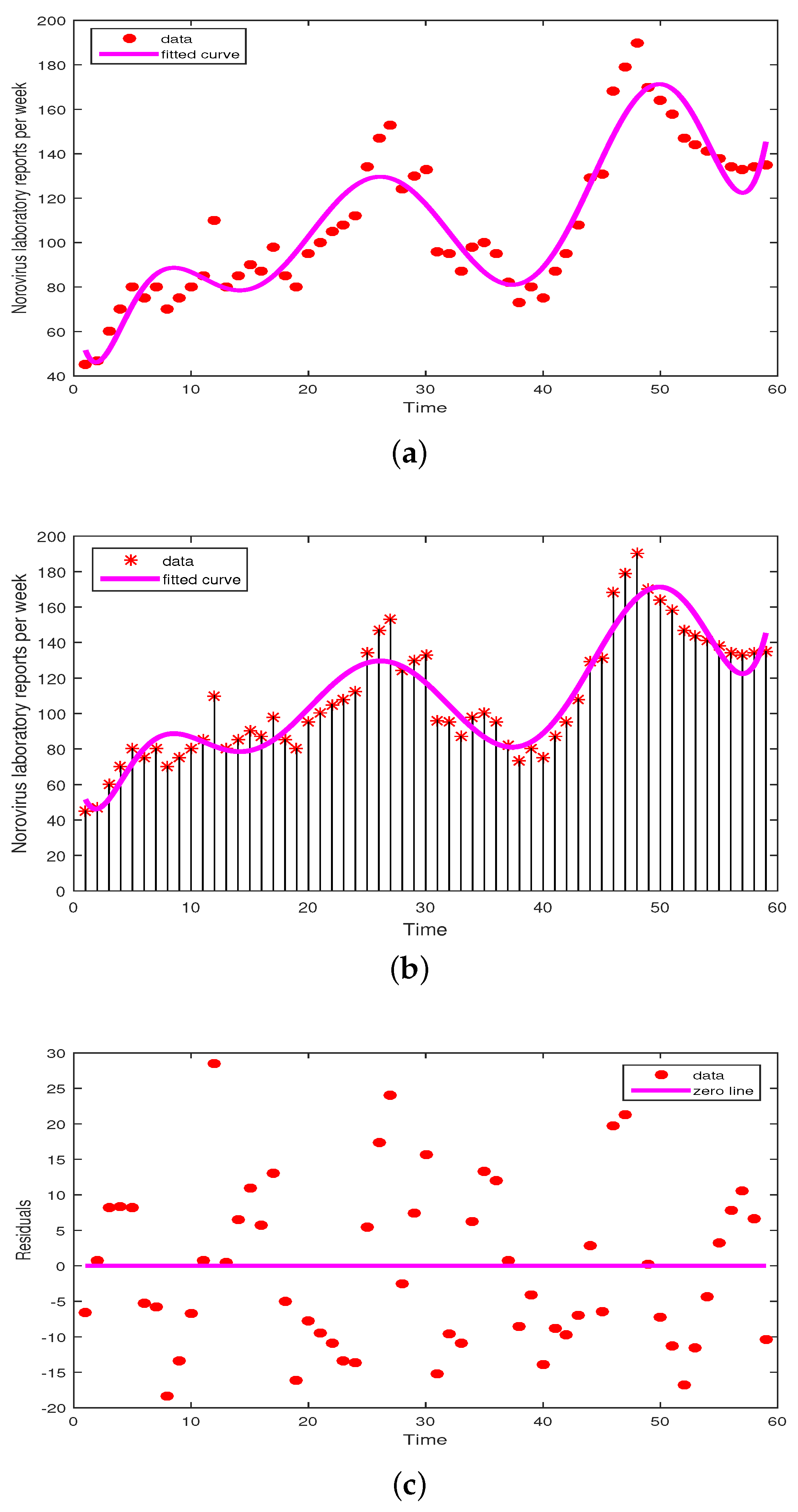
9. Numerical Simulation

In this section of the article, our aim was to find the approximate solution for the non-integer-order NoV (Norovirus) system using the ABC derivative of model (3). The simulation was performed over a time interval ranging from 0 to 60 steps, utilizing MATLAB 2019. The system parameters are provided in

Table 1. The table represents the parameters values and initial conditions of the state variable given in model (1).

Parameters	Description	Value	Source
$\mathsf{\Lambda }$	The recruitment rate	125.66/day	Fitted
$\eta$	The rate of effectively contacts	0.02/day	Estimated
$\rho$	The vaccinated converging rate	0.01/day	Estimated
d	The natural mortality rate	0.02/day	Estimated
$\delta$	The recovery rate	0.5/day	Estimated
$\alpha$	Developing clinical symptoms	0.2/day	[38]
$\tau$	The vaccine efficiency	0.90/day	Estimated
$\mathcal{H}\left(0\right)$	IC	75	[38]
$\mathcal{V}\left(0\right)$	IC	20	[38]
$\mathcal{U}\left(0\right)$	IC	55	[38]
$\mathcal{A}\left(0\right)$	IC	30	[38]
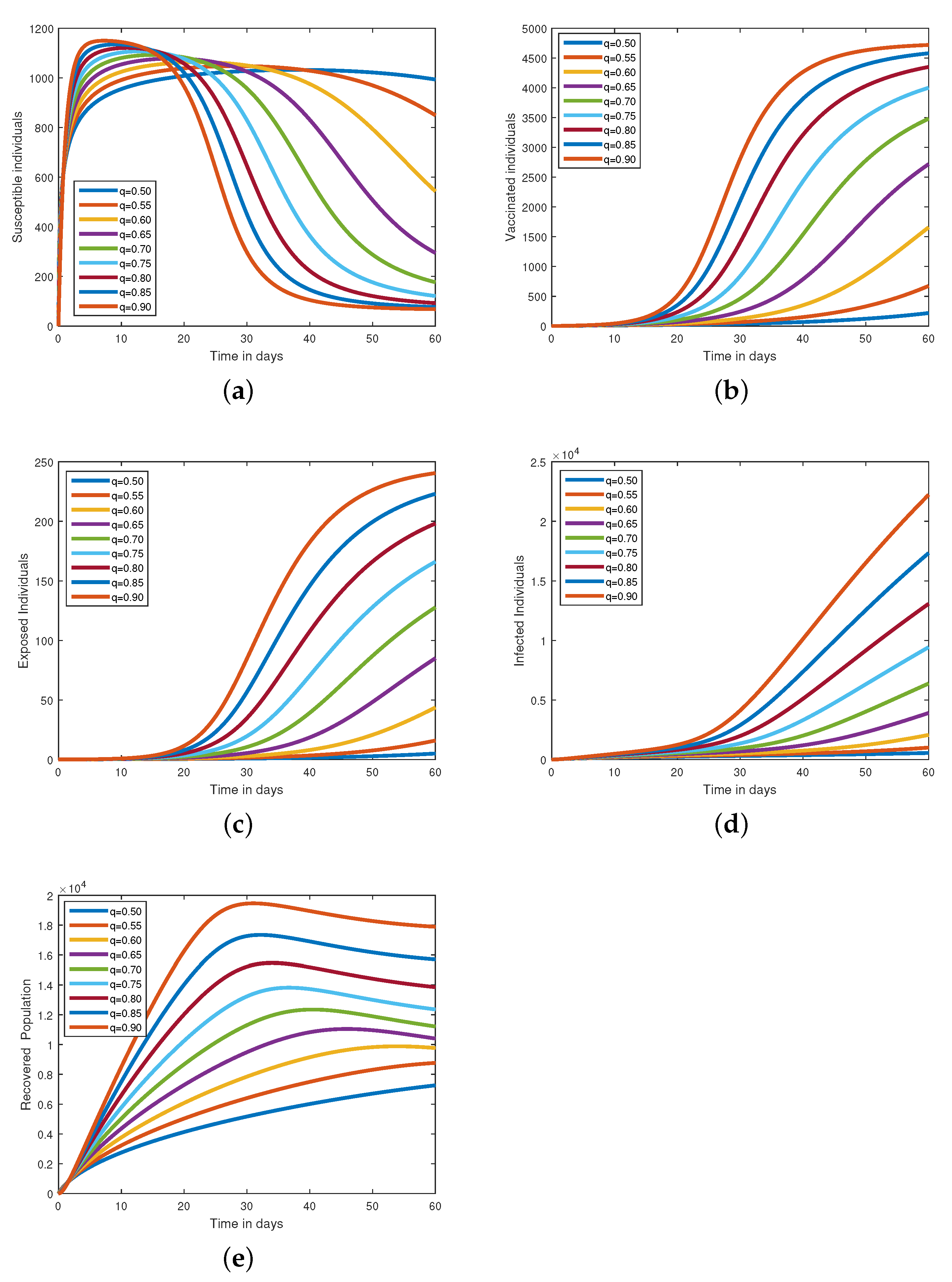
$\mathcal{C}\left(0\right)$	IC	20	[38]

, and these values are used for graphical representation. The numerical simulation was conducted for various orders of q, and the results indicate that the non-integer-order fractional derivative yields favorable outcomes for controlling the infected class. The dynamics of each class in the system (3), for different values of q such as $0.90,0.85,0.80,0.75,0.70,0.65,0.60,0.55,0.50$, are depicted in Figure 4a–e. Figure 4a illustrates an increasing trend in the number of healthy individuals with a decay occurring in the fractional order q. Figure 4c demonstrates the growth of the exposed class for arbitrary values of q; however, after a certain time interval (around 20), the exposed class starts to decrease. The population of the infected class decreases over time as the values of q decrease in Figure 4d. Additionally, Figure 4b illustrates how newborns can immunize themselves by being carried by their mothers. This implies that proper care for carrier mothers could result in the vaccination-induced recovery of newborns in as little as a day. Similar to this, Figure 4e represents the recovery class and illustrates how people recover from infections. 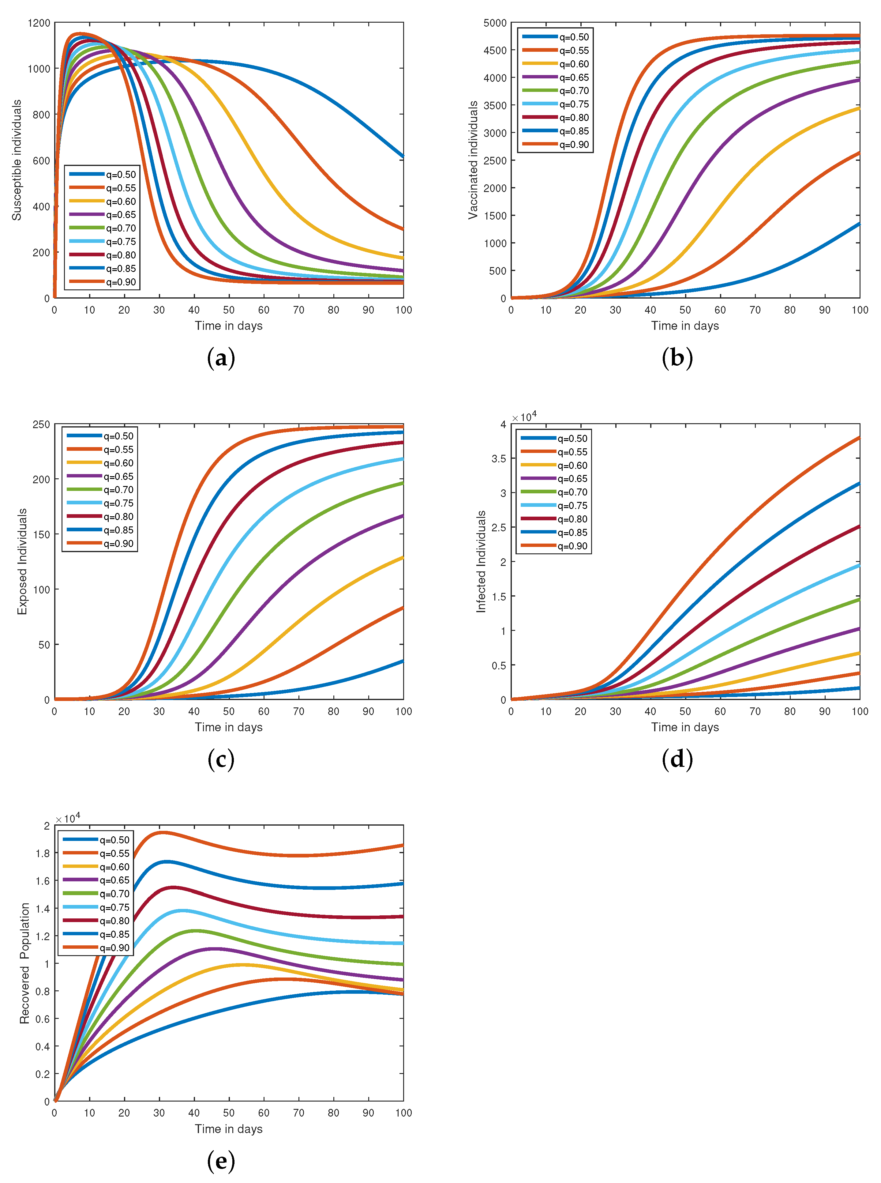The approximative results show clear system deviations for various non-integer order parameter q values. 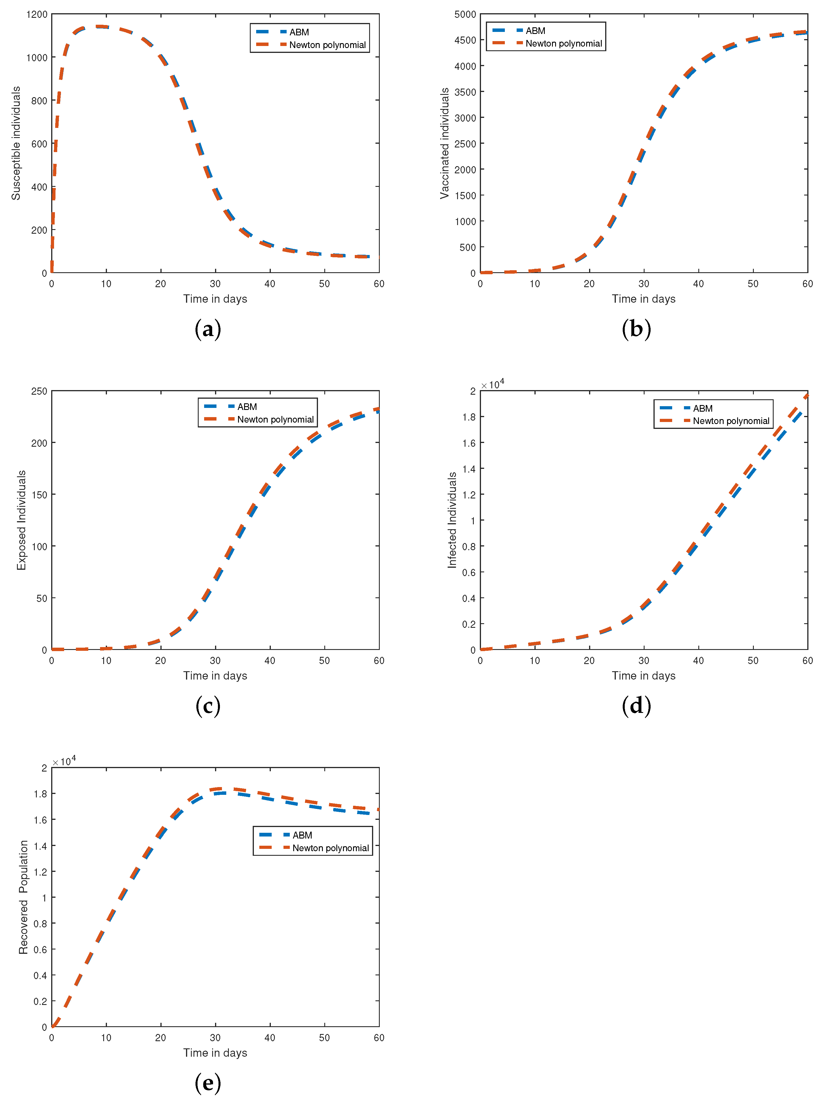The long-term simulation results obtained using ABM methods are also shown in Figure 5. Additionally, Figure 6 compares the simulation outcomes attained using the Newton polynomial and ABM approaches. 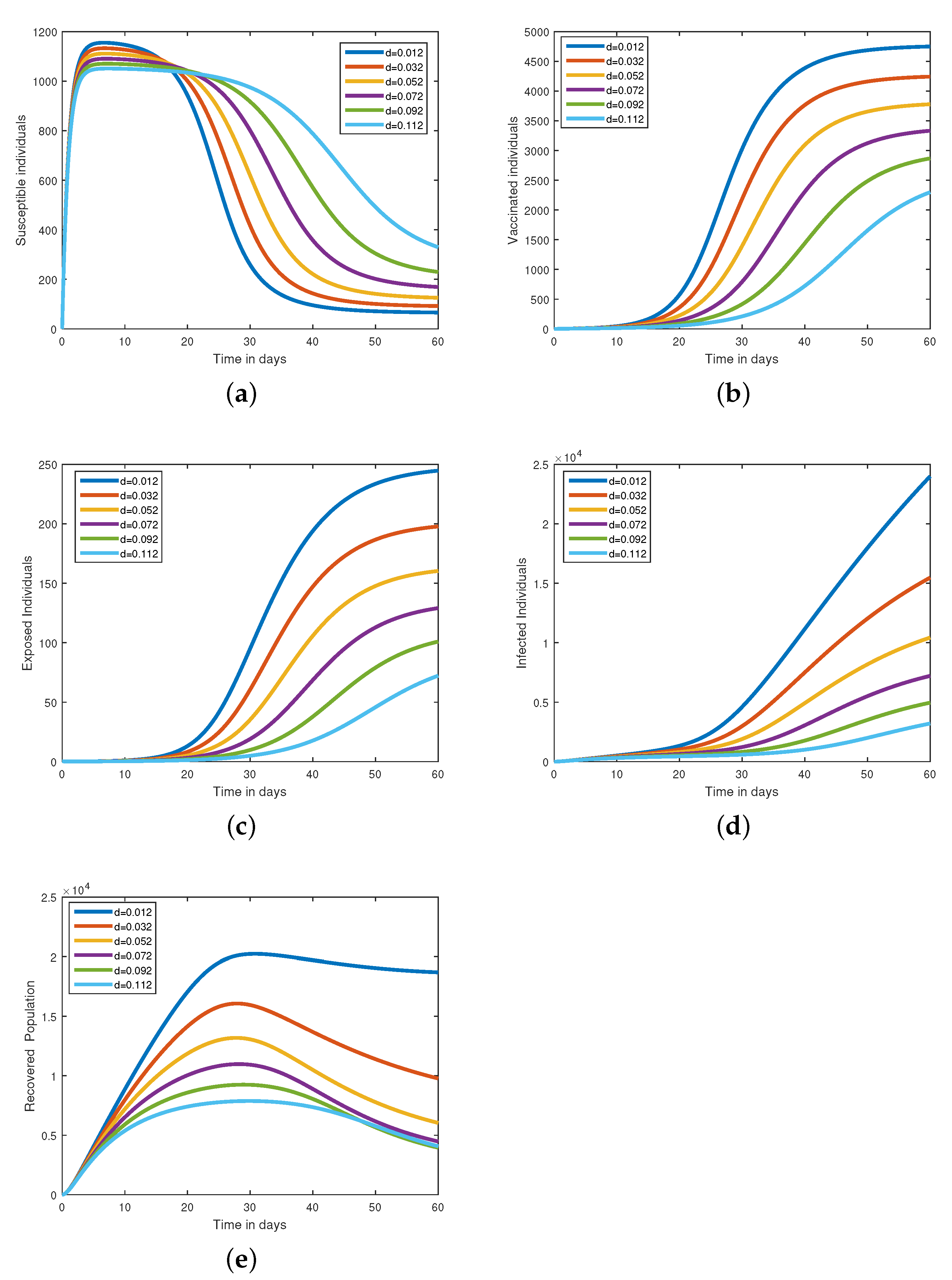Figure 7 and Figure 8 show the simulation results specifically for the Newton polynomial method. Additionally, Figure 9 and Figure 10 show, for each state variable, the effects of the transmission parameter $eta$ and the natural removal rate d, respectively, on the results of the simulation.

10. Conclusions

In this paper, we have conducted a thorough investigation into the dynamics of Norovirus (NoV), taking into account the presence of asymptomatic carriers and the effects of vaccination. Our study utilized the Atangana–Baleanu–Caputo (ABC) fractional order derivative and applied fixed point theory to derive qualitative analysis for the positive solution of the system. To obtain an approximate solution, we have employed an iterative numerical method. Furthermore, we have presented graphical results for each system quantity at different fractional orders, revealing a convergence of curves to the integer order curves as the order increases. Our findings demonstrate a significant reduction in the number of infected cases through vaccination, emphasizing its positive impact. Consequently, this article provides valuable guidance for public health authorities in promoting and ensuring widespread vaccination within communities. Educating both rural and urban areas about the importance of vaccination and proper treatment is crucial for effectively controlling and preventing NoV outbreaks. The use of Atangana–Baleanu fractional derivatives demonstrates their usefulness as a tool for researching the dynamics of norovirus disease transmission, and our work highlights several crucial features of the fractional model. These include the model’s creation, the fixed-point theorem’s proof of the existence and uniqueness of solutions, stability and sensitivity analyses, and the basic reproduction number. Notably, the basic reproduction number is most sensitive to the disease transmission rate ($\eta$), whereas the basic reproduction number is least sensitive to the natural mortality rate (d) and the recovery rate of isolated individuals ($\delta$). Additionally, because an increase in the fractional parameter results in an overall increase in the indices of all parameters, the fractional parameter has a significant impact on the sensitivity indices.

References

1. Ahmed, S.M.; Lopman, B.A.; Levy, K. A systematic review and meta-analysis of the global seasonality of norovirus. PLoS ONE 2013, 8, 75922. [Google Scholar] [CrossRef] [PubMed]
2. Marshall, J.A.; Bruggink, L.D. The dynamics of norovirus outbreak epidemics: Recent insights. Int. J. Environ. Res. Public Health 2011, 8, 1141–1149. [Google Scholar] [CrossRef] [PubMed] [Green Version]
3. Rohayem, J. Norovirus seasonality and the potential impact of climate change. Clin. Microbiol. Infect. 2009, 18, 524–527. [Google Scholar] [CrossRef] [PubMed] [Green Version]
4. Carmona-Vicente, N.; Fernández-Jiménez, M.; Ribes, J.M. Norovirus infections and seroprevalence of genotype GII.4–Specific antibodies in a Spanish population. J. Med. Virol. 2015, 8, 675–682. [Google Scholar] [CrossRef]
5. Anwarud, D.; Li, Y. Stochastic optimal control for norovirus transmission dynamics by contaminated food and water. Chin. Phys. B 2021, 31, 020202. [Google Scholar]
6. Hossein, J.; Daftardar-Gejji, V. Solving linear and nonlinear fractional diffusion and wave equations by Adomian decomposition. Appl. Math. Comput. 2006, 180, 488–497. [Google Scholar]
7. Li, X.-P.; Wang, Y.; Khan, M.A.; Alshahrani, M.Y.; Muhammad, T. A dynamical study of SARS-CoV-2: A study of third wave. Results Phys. 2021, 29, 104705. [Google Scholar] [CrossRef]
8. Razia, B.; Tunç, O.; Khan, H.; Gulzar, H.; Khan, A. A fractional order Zika virus model with Mittag–Leffler kernel. Chaos Solitons Fractals 2021, 146, 110898. [Google Scholar]
9. Osman, T.; Tunç, C. Ulam stabilities of nonlinear iterative integro-differential equations. Rev. Real Acad. Cienc. Exactas Físicas Nat. Ser. Matemáticas 2023, 117, 118. [Google Scholar]
10. Muhammad Shoaib, A.; Raza, A.; Rafiq, M.; Bibi, M. A reliable numerical analysis for stochastic hepatitis B virus epidemic model with the migration effect. Iran. J. Sci. Technol. Trans. A Sci. 2019, 43, 2477–2492. [Google Scholar]
11. Lu, Q. Stability of SIRS system with random perturbations. Phys. A Stat. Mech. Its Appl. 2009, 388, 3677–3686. [Google Scholar] [CrossRef]
12. Liu, P.; Din, A.; Zarin, R. Numerical dynamics and fractional modeling of hepatitis B virus model with non-singular and non-local kernels. Results Phys. 2022, 39, 105757. [Google Scholar] [CrossRef]
13. Zhang, X.-B.; Wang, X.-D.; Huo, H.-F. Extinction and stationary distribution of a stochastic SIRS epidemic model with standard incidence rate and partial immunity. Phys. A Stat. Mech. Its Appl. 2019, 531, 121548. [Google Scholar] [CrossRef]
14. Raizah, Z.; Zarin, R. Advancing COVID-19 Understanding: Simulating Omicron Variant Spread Using Fractional-Order Models and Haar Wavelet Collocation. Mathematics 2023, 11, 1925. [Google Scholar] [CrossRef]
15. Simone, G.; Fusè, M.; Mazzeo, G.; Abbate, S.; Longhi, G. MCD and Induced CD of a Tetraphenoxyperylene-Based Dye in Chiral Solvents: An Experimental and Computational Study. Symmetry 2023, 14, 1108. [Google Scholar] [CrossRef]
16. Zarin, R.; Khaliq, H.; Khan, A.; Ahmed, I. and Humphries, U.W. A numerical study based on haar wavelet collocation methods of fractional-order antidotal computer virus model. Symmetry 2023, 15, 621. [Google Scholar] [CrossRef]
17. Hossein, J.; Daftardar-Gejji, V. Solving a system of nonlinear fractional differential equations using Adomian decomposition. J. Comput. Appl. Math. 2006, 196, 644–651. [Google Scholar]
18. Hossein, J.; Yousefi, S.A.; Firoozjaee, M.A.; Momani, S.; Masood Khalique, C. Application of Legendre wavelets for solving fractional differential equations. Comput. Math. Appl. 2011, 62, 1038–1045. [Google Scholar]
19. Khan, A.; Zarin, R.; Humphries, U.W.; Akgül, A.; Saeed, A.; Gul, T. Fractional optimal control of COVID-19 pandemic model with generalized Mittag-Leffler function. Adv. Differ. Equ. 2021, 2021, 387. [Google Scholar] [CrossRef]
20. Khan, A.; Zarin, R.; Hussain, G.; Ahmad, N.A.; Mohd, M.H.; Yusuf, A. Stability analysis and optimal control of COVID-19 with convex incidence rate in Khyber Pakhtunkhawa (Pakistan). Results Phys. 2021, 20, 103703. [Google Scholar] [CrossRef]
21. Hossein, J.; Masood Khalique, C.; Nazari, M. Application of the Laplace decomposition method for solving linear and nonlinear fractional diffusion–Wave equations. Appl. Math. Lett. 2011, 24, 1799–1805. [Google Scholar]
22. Hossein, Y.; Daftardar-Gejji, V. Revised Adomian decomposition method for solving systems of ordinary and fractional differential equations. Appl. Math. Comput. 2006, 181, 598–608. [Google Scholar]
23. Shen, H.; Chu, Y.-M.; Khan, M.A.; Muhammad, S.; Al- Hartomy, O.A.; Higazy, M. Mathematical modeling and optimal control of the COVID-19 dynamics. Results Phy. 2021, 31, 105026. [Google Scholar] [CrossRef]
24. Zarin, R.; Khan, A.; Inc, M.; Humphries, U.W.; Karite, T. Dynamics of five grade leishmania epidemic model using fractional operator with Mittag–Leffler kernel. Chaos Solitons Fractals 2021, 147, 110985. [Google Scholar] [CrossRef]
25. Abdon, A.; Baleanu, D. New fractional derivatives with nonlocal and non-singular kernel: Theory and application to heat transfer model. arXiv 2016, arXiv:1602.03408. [Google Scholar]
26. Abdon, A.; Koca, I. Chaos in a simple nonlinear system with Atangana–Baleanu derivatives with fractional order. Chaos Solitons Fractals 2016, 89, 447–454. [Google Scholar]
27. Gu, Y.; Khan, M.; Zarin, R.; Khan, A.; Yusuf, A.; Humphries, U.W. Mathematical analysis of a new nonlinear dengue epidemic model via deterministic and fractional approach. Alex. Eng. J. 2023, 67, 1–21. [Google Scholar] [CrossRef]
28. Hossein, J.; Nazari, M.; Baleanu, D.; Masood Khalique, C. A new approach for solving a system of fractional partial differential equations. Comput. Math. Appl. 2013, 66, 838–843. [Google Scholar]
29. Afshin, B.; Jafari, H.; Ahmadi, M. A fractional order HIV/AIDS model based on the effect of screening of unaware infectives. Math. Methods Appl. Sci. 2019, 42, 2334–2343. [Google Scholar]
30. Anwarud, D.; Li, Y.; Muhammad Khan, F.; Ullah Khan, Z.; Liu, P. On Analysis of fractional order mathematical model of Hepatitis B using Atangana–Baleanu Caputo (ABC) derivative. Fractals 2022, 30, 2240017. [Google Scholar]
31. Anwarud, D.; Li, Y.; Yusuf, A.; Isa Ali, A. Caputo type fractional operator applied to Hepatitis B system. Fractals 2022, 30, 2240023. [Google Scholar]
32. Can, N.H.; Nikan, O.; Rasoulizadeh, M.N.; Jafari, H.; Gasimov, Y.S. Numerical computation of the time non-linear fractional generalized equal width model arising in shallow water channel. Therm. Sci. 2020, 24 (Suppl. S1), 49–58. [Google Scholar] [CrossRef]
33. Salama, F.M.; Ali, N.H.M.; Abd Hamid, N.N. Fast O (N) hybrid Laplace transform-finite difference method in solving 2D time fractional diffusion equation. J. Math. Comput. Sci. 2021, 23, 110–123. [Google Scholar] [CrossRef]
34. Jassim, H.K.; Shareef, M.A. On approximate solutions for fractional system of differential equations with Caputo-Fabrizio fractional operator. J. Math. Comput. Sci. 2021, 23, 58–66. [Google Scholar] [CrossRef]
35. Akram, T.; Abbas, M.; Ali, A. A numerical study on time fractional Fisher equation using an extended cubic B-spline approximation. J. Math. Comput. Sci. 2021, 22, 85–96. [Google Scholar] [CrossRef]
36. Colin, S.; Edgar, W.; Simard, P.; Finelli, L.; Fiore, A.E.; Bell, B.P. Hepatitis B virus infection: Epidemiology and vaccination. Epidemiol. Rev. 2006, 28, 112–125. [Google Scholar]
37. Shapiro, C.N. Epidemiology of hepatitis B. Pediatr. Infect. Dis. J. 1993, 12, 433–437. [Google Scholar] [CrossRef] [Green Version]
38. Ting, C.; Liu, P.; Din, A. Fractal–fractional and stochastic analysis of norovirus transmission epidemic model with vaccination effects. Sci. Rep. 2021, 11, 1–25. [Google Scholar]
39. Biazar, J. Solution of the epidemic model by Adomian decomposition method. Appl. Math. and Comp. 2006, 173, 1101–1106. [Google Scholar] [CrossRef]
40. Rafei, M.; Ganji, D.D.; Daniali, H. Solution of the epidemic model by homotopy perturbation method. Appl. Math. and Comp. 2007, 187, 1056–1062. [Google Scholar] [CrossRef]
41. Ahmed, A. Adomian Decomposition Method: Convergence Analysis and Numerical Approximation. Master’s Thesis, McMaster University, Hamilton, ON, USA, 2008. [Google Scholar]
42. Ali, Z.; Zada, A.; Shah, K. Ulam stability to a toppled systems of nonlinear implicit fractional order boundary value problem. Bound. Value Probl. 2018, 175, 1–16. [Google Scholar] [CrossRef] [Green Version]
43. National Norovirus and Rotavirus Report, Week 4 Report: Data up to Week 2 (15 January 2023). Available online: https://www.gov.uk/government/statistics/national-norovirus-and-rotavirus-surveillance-reports-2022-to-2023-season/national-norovirus-and-rotavirus-report-week-4-report-data-up-to-week-2-15-january-2023 (accessed on 23 August 2022).
Figure 1. Schematic diagram of the model.
Symmetry 15 01208 g001
Figure 2. The plots examine how changes in various parameters relate to R 0 through sensitivity analysis. (a) R 0 versus sensitive parameters d and α . (b) R 0 versus sensitive parameters ρ and α . (c) R 0 versus sensitive parameters Λ and τ . (d) R 0 versus sensitive parameters τ and d. (e) R 0 versus sensitive parameters α and Λ . (f) R 0 versus sensitive parameters δ and d.
Symmetry 15 01208 g002
Figure 3. The graph presents the optimized curve that best fits the data, along with the residuals depicting the discrepancies between the simulated results and the recorded daily cumulative cases within the corresponding timescale. (a,b) Represents the model fit with the Norovirus laboratory-reported cases per week, and (c) represents the Residuals.
Symmetry 15 01208 g003
Figure 4. Paths for the solution of system (3) for t = 60, when q = 0.90, 0.85, 0.80, 0.75, 0.70, 0.65, 0.60, 0.55, 0.50. (a) Susceptible individuals. (b) Vaccinated individuals. (c) Exposed individuals. (d) Infected individuals. (e) Recovered individuals.
Symmetry 15 01208 g004
Figure 5. Paths for the solution of system (3) for a long time t = 100, when q = 0.90, 0.85, 0.80, 0.75, 0.70, 0.65, 0.60, 0.55, 0.50. (a) Susceptible individuals. (b) Vaccinated individuals. (c) Exposed individuals. (d) Infected individuals. (e) Recovered individuals.
Symmetry 15 01208 g005
Figure 6. The plots represents the caparison of ABM and Newton’s polynomial numerical methods on each state variable at fractional order q = 0.95 . (a) Susceptible individuals. (b) Vaccinated individuals. (c) Exposed individuals. (d) Infected individuals. (e) Recovered individuals.
Symmetry 15 01208 g006
Figure 7. Paths for the solution of system (3) via Newton’s Polynomial numerical method for a long time t = 60, when q = 0.90, 0.85, 0.80, 0.75, 0.70, 0.65, 0.60, 0.55, 0.50. (a) Susceptible individuals. (b) Vaccinated individuals. (c) Exposed individuals. (d) Infected individuals. (e) Recovered individuals.
Symmetry 15 01208 g007
Figure 8. Paths for the solution of system (3) via Newton’s Polynomial numerical method for a long time t = 100, when q = 0.90,0.85,0.80,0.75, 0.70, 0.65, 0.60, 0.55, 0.50. (a) Susceptible individuals. (b) Vaccinated individuals. (c) Exposed individuals. (d) Infected individuals. (e) Recovered individuals.
Symmetry 15 01208 g008
Figure 9. Impact of the parameter η which represent the rate of effectively contacts on each state variable at fractional order q = 1 . (a) Susceptible individuals. (b) Vaccinated individuals. (c) Exposed individuals. (d) Infected individuals. (e) Recovered individuals.
Symmetry 15 01208 g009
Figure 10. Impact of the parameter d which represents the natural death on each state variable at fractional order q = 1 . (a) Susceptible individuals. (b) Vaccinated individuals. (c) Exposed individuals. (d) Infected individuals. (e) Recovered individuals.
Symmetry 15 01208 g010