Incremental Machine Learning for Soft Pneumatic Actuators with Symmetrical Chambers

Abstract

Soft robotics is a specialized field of robotics that focuses on the design, manufacture, and control of robots made of soft materials, as opposed to those made of rigid links. One of the primary challenges for the future use of continuous or hyper-redundant robotics systems in industrial and medical technology is the development of suitable modeling and control approaches. Due to the complex non-linear behavior of soft materials and the unpredictable motion of actuators, the task of modeling complex soft actuators is very time-consuming. As a result, earlier studies have undertaken research into model-free methods for controlling soft actuators. In recent years, machine learning (ML) methods have become widely popular in research. The adaptability of an ML model to a non-linear soft drive system alongside the varying actuation behavior of soft drives over time as a result of material characteristics and performance requirements is the key rationale for including an ML model. The system requires the online updating of the ML model in order to work with the non-linear system. Sequential data collected from the test bench and converted into a hypothesis are used to perform incremental learning. These methods are called lifelong learning and progressive learning. Real-time data flow training is combined with incremental learning (IL), and a neural network model is tuned sequentially for each data input. In this article, a method for the intelligent control of soft pneumatic actuators based on an incremental learning algorithm is proposed. A soft pneumatic actuator was subjected to three distinct test conditions in a controlled test environment for a specified duration of data gathering. Additionally, data were collected through finite element method simulations. The collected data were used to incrementally train a neural network, and the resulting model was analyzed for errors with both training and test data. The training and testing errors were compared for different incremental learning (IL) algorithms, including K-nearest neighbors, a decision tree, linear regression, and a neural network. The feasibility of the modulo-free intelligent control of soft pneumatic actuators based on an incremental learning algorithm was verified, solving the problem of the control of software actuators.

1. Introduction

Robot technology is widely used in industrial production, exploration and survey, medical service, military reconnaissance, and other fields, which is of great significance to the national economy and national defense construction. From the perspective of the basic materials used, current robots can be divided into two types: rigid-body robots and soft-body robots. Traditional rigid-body robots are mostly composed of rigid kinematic pairs based on hard materials (such as metals, plastics, etc.), which can quickly and accurately complete work tasks. The most widely used rigid-body robots in industrial production are non-redundant in terms of kinematics [1]. The multiple kinematic joints of such a robot are rigidly connected, and each joint provides the robot with a degree of freedom of rotation or linear motion. The reachable range of all degrees of freedom constitutes the working space of the robot and also determines all the positions that the end-effector can reach. However, this traditional robot has limited flexibility and low environmental adaptability, and can only work in a structured environment, which limits the application of rigid robots in dynamic, unknown, and unstructured complex environments, such as military reconnaissance, disaster relief, scientific exploration, etc. When the number of joints of a rigid robot continues to increase, the robot has redundancy or even super-redundancy, which greatly improves the robot’s dexterity. The environmental adaptability of this kind of robot is improved compared with a robot without redundancy, but its body is still composed of hard materials, and the size and size cannot be changed arbitrarily. When it is applied in a specific environment, it needs to provide advance information, such as the shapes and sizes of obstacles.

Compared with rigid-body robots, soft-body robots have more degrees of freedom and can realize more motion modes, which makes soft-body robots have certain advantages in terms of flexibility, but it also raises new problems, such as how to control soft-body robots’ position perception, how to improve the controllability of soft robots, how to improve the load capacity of soft structures, etc. In the past 10 to 20 years, researchers around the world have developed a variety of soft robots, which have realized some functions that were difficult or difficult to achieve with traditional robots, such as slit crawling, continuous swimming, flexible grasping, etc. Usually, the design inspiration for soft robots comes from organisms or biological tissues in nature, such as caterpillars, starfish, octopus tentacles, and so on. This is because mollusks or animal soft tissues have undergone natural evolution for hundreds of millions of years and have the characteristics of large deformations, light weights, and high power–density ratios, which can make them more efficient under complex natural environmental conditions by changing their body shapes. By studying the movement patterns, epidermis structure, and muscle contraction methods of mollusks, researchers have used methods such as physics, chemistry, and material properties to realize biological movements [2].

At present, robotics and automation processes are widely integrated into all technological processes, including vehicle motion control [3], indoor and outdoor automated localization and mapping [4,5], computer vision systems [6,7,8], machine learning [9,10], and neural networks [11,12], and are definitely increasing the efficiency of technological processes.

Soft robotics is a subfield that deals with the creation and control of resilient robots and that takes cues from soft-bodied animals. The designs of soft robots are based on the anatomies of soft-bodied organisms such as octopuses, elephant trunks, snakes, etc., using the influence of nature and creating very complex and advanced environmental designs for the movement of biotechnology-inspired robots [13]. Numerous structures are being studied and developed in the design and development of soft robots (SRs) that can solve any problem that arises in everyday life. Because of their softness, these robots can be used in dangerous environments [14].

The field of soft robotics has evolved with numerous design and control strategies and is now struggling with control problems caused by the viscoelastic nature of these robots [15]. Due to their brittleness and ease of fabrication, silicone forms are the basis of the SR architecture.

In recent years, SRs have also found applications in the field of medicine [16,17], including surgery and the implantation of prosthetic limbs for disabled people. The two main areas of research on SRs are design and control, with design proving to be more complex than with traditional hard-material robots. In many educational and industrial institutions, an innovative control system that pushes the boundaries for soft robot control is an attractive issue [18,19,20]. The main component that should be in an SR is an actuation system, which helps to produce the output needed to interact with the environment. There are many methods that are superior for demonstrating the effectiveness of an SR based on its viscoelastic behavior.

Considering that electric drives are generally more expensive and heavier than pneumatic or thermal drives, they also have lower power density. In addition, electric and thermal drives may heat up during operation and require cooling or dissipation, which makes these systems complicated, while pneumatic drives are generally simpler, cheaper, and lighter than electric motors. They can also provide higher power density and speed compared with electric motors. Moreover, a pneumatic drive device can be used to operate in dangerous or adverse environments, such as in high temperatures, radiation, chemically corrosive environments, etc. This experiment chose pneumatic drives.

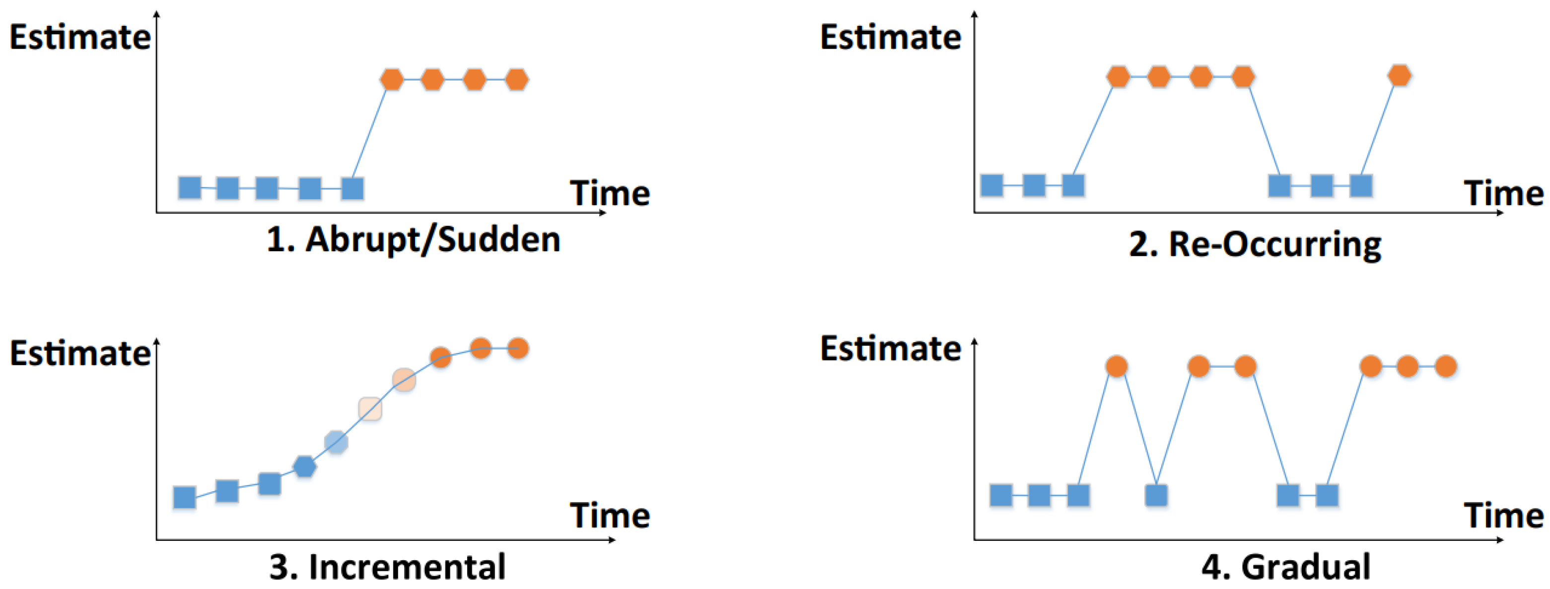
The non-linear and hysteresis behavior of soft actuators has been briefly discussed in the literature [21]. Non-linearity refers to the relationship between the input and output characteristics of a system. Hysteresis, drift, and additional degrees of freedom all contribute to the non-linearity of a system, making it complicated to control the actuator. Machine learning techniques have been proven to be effective in addressing these issues by providing solutions to complex systems in various domains. Various learning-based control techniques have been proposed, and the challenges related to temporal behavior have been explained [22], with specific machine learning models used in state-of-the-art control techniques. In comparison with Jacobian-based methods for soft actuators, the feed-forward neural network (FNN) has been found to outperform in terms of system accuracy. However, the difficulty of adapting systems to non-linearity remains since static machine learning is not suitable for systems with changing behavior. Therefore, learning-based approaches such as reinforcement learning and online incremental learning are gaining prominence in the field of soft robotics. In this article, we tried to use online incremental learning to address the limitations of soft actuators in control problems; compare the training and testing errors of the K-nearest neighbors, decision tree, linear regression, and neural network algorithms; and compare the results via comparative analysis. The experiments proved that it can achieve the predetermined model-free control effect.

2. Materials and Methods

This chapter mainly studies the design of the system model, the training method of the model, and the testing method of the model. It also discusses the feasibility, advantages, and disadvantages of the four model design methods. The differences between the four model training methods show the structure and rationality of the system test. In general, in this chapter, we first analyze the reasons and purposes for choosing the K-nearest neighbors regressor, a decision tree regressor, linear regression, and a neural network, and then we theoretically analyze the advantages and disadvantages of batch learning and incremental learning and choose the most suitable for the incremental learning training method of this experiment, and then we carry out pre-training and non-pre-training tests using the method of incremental learning. Finally, we obtain the training errors of the four models in the training group and the test errors in the test group, which are included in the following results analysis providing the data basis.

2.1. Model-Related Algorithms

In this article, it was necessary to use the incremental learning method for adaptive training. Among the algorithms suitable for incremental learning, the K-nearest neighbors algorithm is fast enough to process new data. It does not require an explicit training process and can perform classification, regression, clustering, etc. In addition, the K-nearest neighbors algorithm can also adapt to different data distributions and has good robustness for non-linear data. The decision tree algorithm can handle datasets with multiple categories and multiple features, and it also has good interpretability and visibility. Decision trees are also able to handle missing and noisy data and can quickly process large-scale datasets. Linear regression can predict continuous values, deal with multiple regression problems, and also has good robustness for high-dimensional datasets and explains the relationships between each feature in these datasets and the target variables. The neural network algorithm can handle complex non-linear models, has better performance for high-dimensional datasets, and can perform end-to-end learning. In addition, the neural network algorithm also has a good generalization ability and can handle missing and noisy data. The four methods discussed above are all in line with the non-linearity, data discontinuity, and noise characteristics of the experimental model.

2.1.1. K-Nearest Neighbors Regressor

The K-nearest neighbors (KNN) [23,24] supervised learning paradigm is non-parametric, and the output of the KNN regressor is the value of the object property, which is the mean of the KNN. The distance calculated from the observed “k” points to a specified point in the dataset is the basis of the KNN method. The number of surrounding points that the model will take into account when estimating a new point is denoted as the letter “k” in the algorithm. The KNN regressor uses the distance between points to determine the output value. There are many approaches that are often used, including the Manhattan distance method and the Euclidean distance method. The choice of method will almost certainly depend on the use case, and each method will affect higher-dimensional data. Due to its efficiency, the Minkowski distance is the most popular distance metric. The equation is shown below.

$$d\left(X,y\right)={{\displaystyle \sum }}_{i=0}^n{({\left|x_i-y_i\right|}^p)}^{1/p}$$

(1)

Depending on the value of p, the formula above represents both the Manhattan distance and the Euclidean distance; if p is 1, it is the Manhattan distance, and if p is 2, it is the Euclidean distance. Based on the vote, each prediction is assigned a weight. Close points will be given more weight than distant points. The algorithm will still consider each of the k-nearest neighbors, but it will ascribe the closer neighbors a larger vote. The MTR problem is handled by the algorithm in the same way.

2.1.2. Decision Tree Regressor

The primary input samples are divided into corresponding homogeneous values for various characteristics using a decision tree (DT) regressor. By segmenting the input features into tiny subsets while maintaining connectivity, the DT builds the model in the form of a branching tree, leaving only decision nodes and end nodes The data are divided according to the characteristic that produces the greatest increase in information, starting from the root node. To solve the model overfitting problem, the split step is repeated at each child node until the leaf nodes are excluded from the DT.

There should be a cost function to optimize the learning tree algorithm to separate nodes according to the most informative features. As can be seen in the equation below, the goal is to maximize the information gained from each split.

$$IG\left(D_p, f\right)=I\left(D_p\right)-\left(\frac{N_{left}}{N_p}I\left(D_{left}\right)+\frac{N_{right}}{N_p}I\left(D_{right}\right)\right)$$

(2)

In the equation above, f denotes the function to perform the split, and D_p, D_left, and D right denote the functions of the parent and child nodes, respectively. I(D_p), I(D_left), and I(D_right) are impurity measures that measure the best separation between a parent node and a subsequent node. N on the left and N on the right refer to the number of samples at the child node, while Np represents the total number of samples at the split node (parent node). The DT used in this experiment works according to the same theory but with additional target predictions.

2.1.3. Linear Regression

For basic problems, linear regression is the most popular and efficient approach. The statistical paradigm for determining the relationship between characteristics with independent inputs and targets with dependent outputs is regression analysis. The equation below provides a broader regression analysis by modeling n data points with one independent variable.

$$y={\beta }_o+{\beta }_1{x}_i+{\epsilon }_i, i=1,2,\dots ,n$$

(3)

The line crossing is represented with ε_i, where β is the parameter and x_i is an independent variable. The experiment model applies the same theory, but it has many output targets, and its function translates these multiple targets into input attributes.

2.1.4. Neural Network

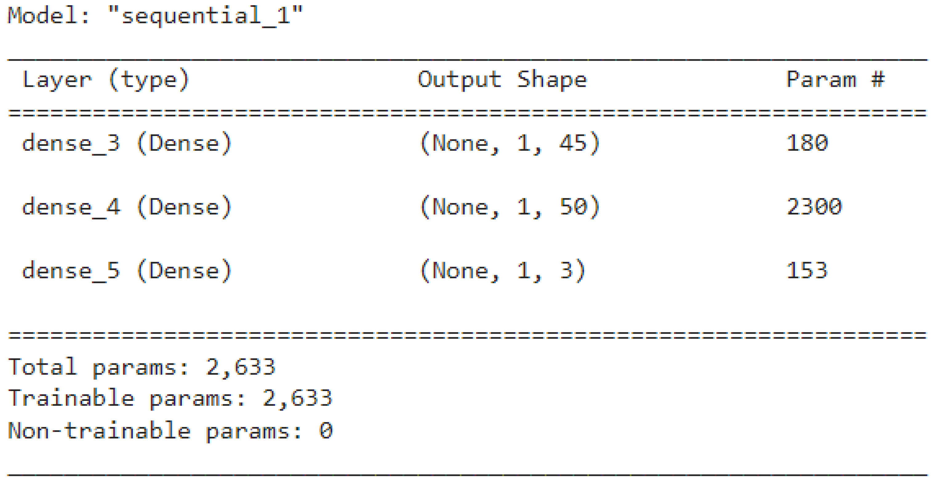
A neural network is an interconnected group of neurons that act like information-storing units, solving highly non-linear problems with less complexity [24]. The architecture of the neural network model is adapted from a previous study on a soft pneumatic actuator [18]. The network consists of 2 hidden layers with 45 and 50 neurons and each of 3 neurons in the input and output. The activation for the input and hidden layers is a hyperbolic tangent activation function and linear activation function in the output layer. Figure 1 below shows the parameter count of the layer structure of the neural network.

2.2. Model Training Type Selection

Neural network training plays a significant role in a machine learning model’s performance, such that training with sufficient data and suitable methods results in an unmatchable output. Gradient descent plays a major role in model training, while weight updating takes place according to the error between the actual and predicted values from the neural network. There are many training methods for a conventional neural network, of which the batch and incremental training methods are discussed below.

Compared with batch training, incremental training first saves computing resources. Incremental learning only needs to update the model when new data arrive, without re-training the entire model. This can save computing resources. The data in this experiment do not exist continuously, which is in line with the incremental learning training method, which allows the model to be directly updated on the existing model without waiting for all the data to arrive before performing batch training. The corresponding speed of volume training is faster, and batch learning is suitable for static datasets. Generally, the training error is extremely low, but the generalization ability is weak. Incremental learning is the opposite. It can be continuously updated and trained. In addition, the generalization ability is stronger, which is suitable for dynamic data. Considering it comprehensively, in this experiment, the incremental learning training method has greater advantages than the batch learning training method.

2.3. Teaching Methods

The performance of a machine learning model is significantly affected by the neural network training process, wherein training with enough data and using the right methods will produce unsurpassed results [25,26,27]. The model is trained primarily with gradient descent, and the weights are updated based on the difference between the actual value and the value predicted by the neural network. There are several training methods for traditional neural networks, among which the batch and incremental training methods are detailed here.

2.3.1. Batch Training

The error for each sample in the training examples is calculated using a gradient descent approach known as batch learning; however, the weight is only updated at the end of each training batch (epoch). Stochastic gradient descent (SGD) [28,29] is a variant of gradient descent used in the River Online Learning Python library. The batch gradient descent algorithm can minimize empirical risk. When the learning rate γ_t is positive and L is the batch size, a continuous estimate w_t of the optimal parameter is obtained. With event zi representing the event indicating the datasets in the batch, and event w t representing the weight to be optimized, Q(z_i, w_t) depicts the loss function.

$$w_{t+1}=w_t-{\gamma }_t \frac{1}{L} {{\displaystyle \sum }}_{i=1}^L{\nabla }_{w}Q\left(z_i,w_t\right)$$

(4)

This approach converges to a local minimum of empirical risk at a small learning rate γ_t. The learning rate γ_t can be modified with an appropriate positive matrix to increase the rate of convergence. There are only a few weight updates during the training phase, which creates a more stable error gradient. A stable error gradient can also lead to higher convergence rates and more generalization of the dataset. When data are available at the earliest stages of model development, a batch training approach is often used.

2.3.2. Additional Training

In order to calculate the error of each sample in the training examples and change the weight of the model, stepwise learning is a type of online gradient descent approach. Because data transformation and model training are performed incrementally using a step-by-step learning approach, algorithms need to be restructured to accommodate changes, as described in the introduction. Using running statistics, where the mean and standard deviation are incrementally updated, the scaling features for streaming data are estimated. x_i, i = 1, m. Given m observations, x_i, i = m + 1, m + n, and a new set of observations also arrives. Taking into account m, the empirical mean at this particular point in time, and n, the empirical mean of the most recent data burst, below is the formula for recursively updating the mean:

$$\mu =\frac{m}{m+n}{\mu }_m+\frac{n}{m+n}{\mu }_n$$

(5)

The empirical variance is given via

$${\sigma }^2=\frac{m}{m+n}{\sigma }_m^2+\frac{m}{m+n}{\sigma }_n^2+\frac{mn}{m+n}{\left({\mu }_m-{\mu }_n\right)}^2$$

(6)

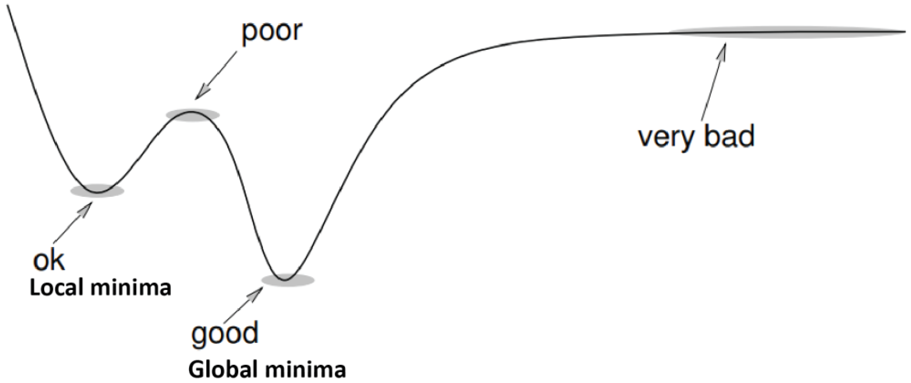
The implementation is easy due to less complex updating of the weights, and noisy data and drifts also tend to create a bad model by avoiding global minima. The cost function is not always convex, as shown in the example in Figure 2 (multiple minima), and the stochastic gradient descent is pruned to miss global minima, and the steps taken to reach the minima are also noisy due to the noisy data. In each step, the calculated gradient is not actual; rather, it is just an approximation of it, so there are a lot of fluctuations in the cost function, leading to a less efficient model [10].

2.3.3. Training and Testing Method

This experiment used incremental learning, which updates the weights for each sample of the training data. Training is an important component of an effective model. The trained model was evaluated for performance using the mean absolute error in each end-effector direction (x, y, z). Because it provides an accurate error rate related to the real output, a mean absolute error matrix was used for this article. 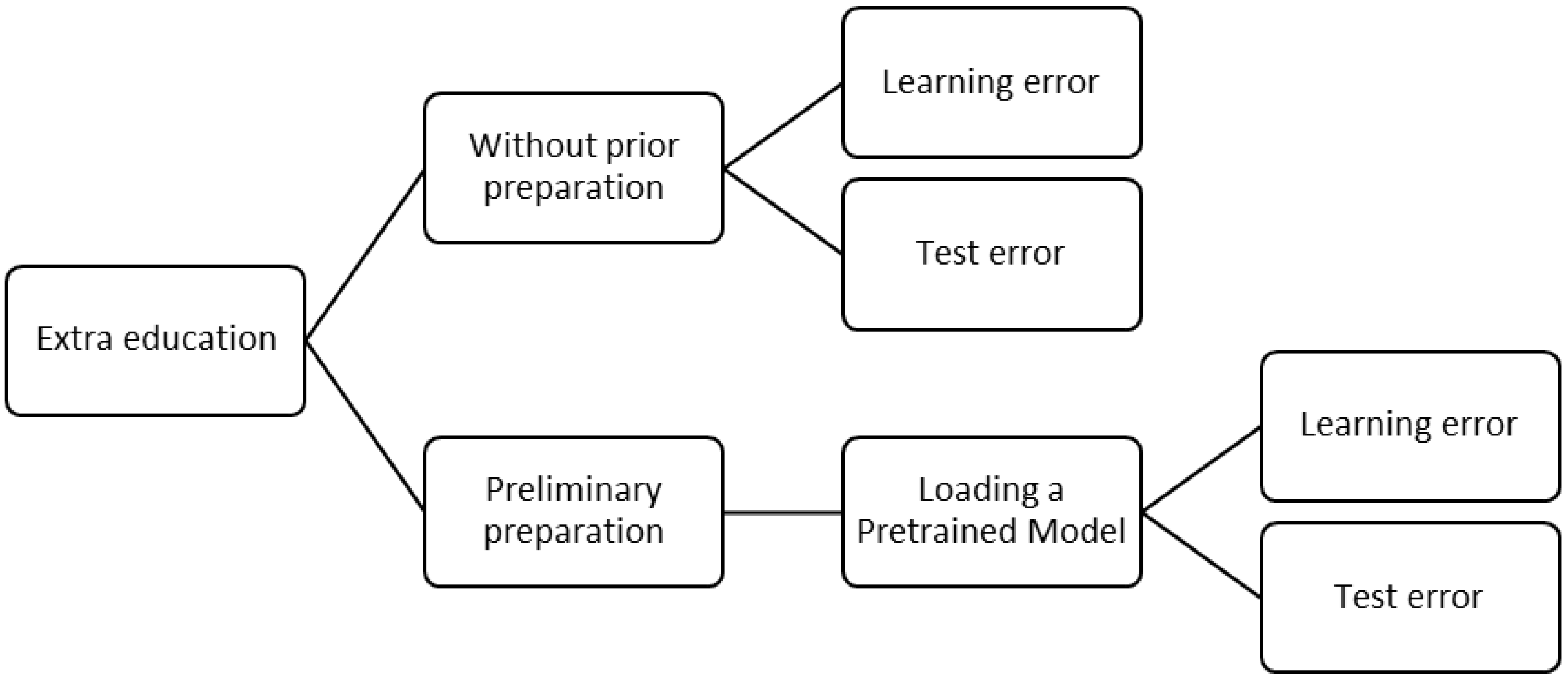As shown in Figure 3, many scenarios were used during training. The goal of this experiment was to develop a model that can predict the location of the end-effector for future data by incrementally learning and storing the model, which can then be used to plan the course of a soft pneumatic actuator. Pre-training and non-pre-training were the two categories into which training was divided.

Figure 3. Training methodology. The model is trained using raw data, predictions are made on the data stream, and training errors are generated to track deviations from true behavior. The trained model is then written in a pickle file format and used to predict the newly discovered data. Training real-time errors and testing errors for undiscovered data are then calculated and compared. This measures the ability of the model to retain information. The method is illustrated in the block diagram in Figure 4.

Figure 3. Training methodology. The model is trained using raw data, predictions are made on the data stream, and training errors are generated to track deviations from true behavior. The trained model is then written in a pickle file format and used to predict the newly discovered data. Training real-time errors and testing errors for undiscovered data are then calculated and compared. This measures the ability of the model to retain information. The method is illustrated in the block diagram in Figure 4.

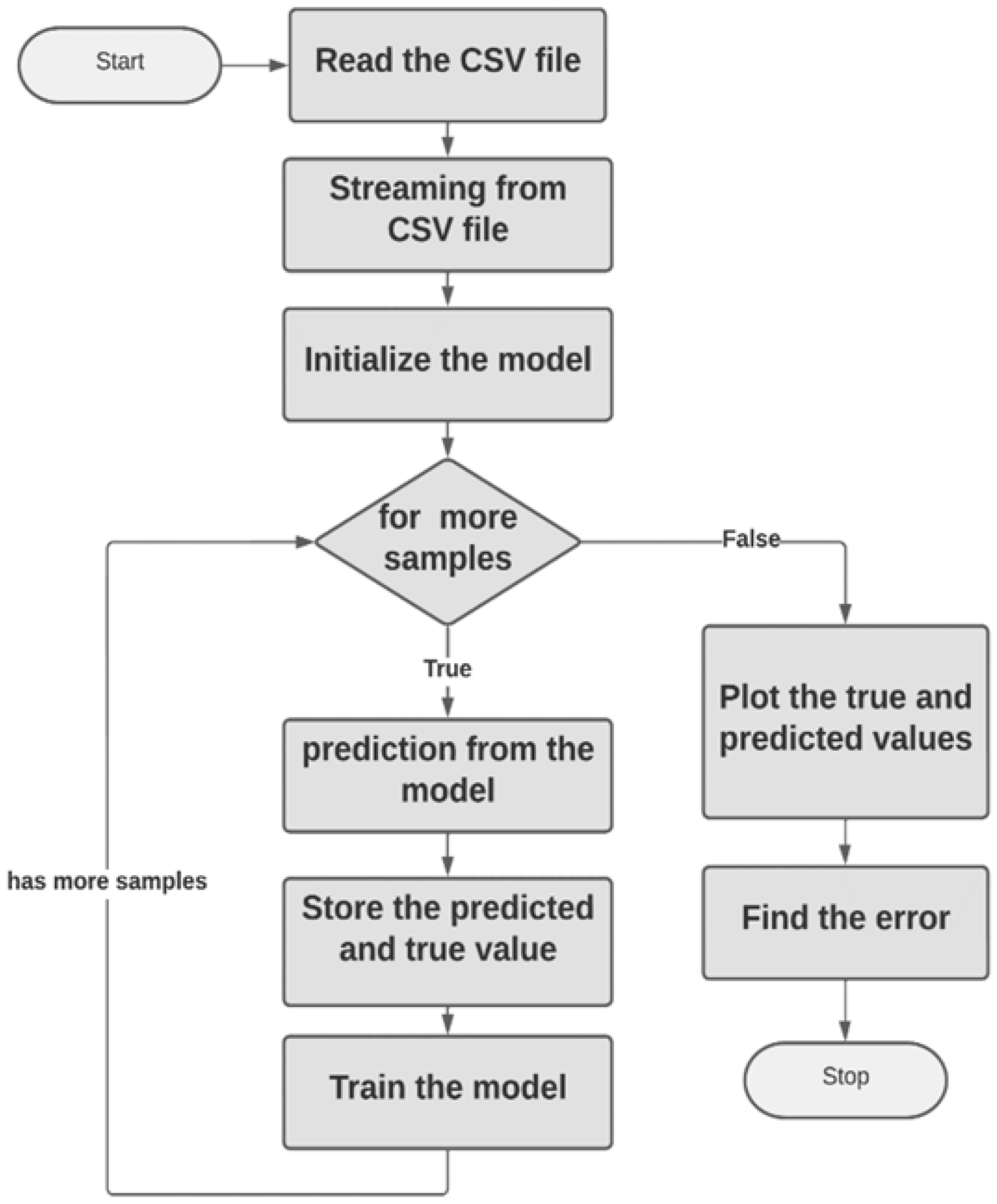
Figure 4. Block diagram of the algorithm.

Figure 4. Block diagram of the algorithm.

2.4. With Pre-Training

When comparing the training with the previous part some minor differences were seen. By using transfer learning, this experiment evaluated the progress in the actual behavior of the model. Batch training was first used to train the model with simulated FEM data, and the pickle file format weights were written. The saved model was then used for additional training after being inserted into the model object. Errors were compared and studied, while the real-time error, training error, and testing error were generated using latent data.

2.5. Ergonomic Methodologies for Modeling and Controlling the Manufacturing Process of Soft Robots

• Design for assembly (DFA): DFA is a methodology used to ensure that components are designed in such a way that they can be easily and quickly assembled. This method takes into account the entire manufacturing process and seeks to reduce the number of steps, components, and labor needed to produce the final product.
• Computer-aided design (CAD): CAD is used to create 3D models of soft robots, allowing engineers to visualize and manipulate their designs before actual production. By utilizing this tool, manufacturers can quickly identify potential problems and make design modifications as needed.
• Process modeling: Process modeling is a technique used to simulate the behavior of a manufacturing process. This method allows engineers to predict how different parameters will affect the final product and make necessary adjustments.
• Simulation-based control: Simulation-based control involves using computer simulations to test and optimize the control systems used to operate soft robots during the manufacturing process. By utilizing this technique, engineers can ensure that their robots are capable of performing their desired tasks with minimal errors or malfunctions.

2.6. Implementation in Python

Python is used to implement machine learning because it has access to a large collection of libraries that are used in data science and machine learning [30,31]. Due to the advantage of allowing a model to adapt to changes in the real world, incremental learning has recently replaced the batch learning paradigm. This incremental learning idea requires building a library from scratch. Because of this desire, the creme and scikit-multiflow libraries were developed, both of which are focused on incremental learning.

Creme and scikit-multiflow teamed up to create a new library known as River. It offers the freedom to stream data from files and supports almost all machine learning and deep learning methods. In addition, the new library offers classes on drift detection, anomaly identification, and more. Any Python-based virtual environment, as well as IDEs, can use the library. In order to train and plot data, coding is performed in a Google Colab notebook, because without a GPU, it would take too long. The block diagram of the program is shown in the figure below. The Google Keras library, which offers user-friendly and less complex code structures compared with other libraries such as TensorFlow and PyTorch, is used for incremental deep-learning-based programming [32,33].

3. Experimental Setups

3.1. Drive

An isometric and cross-sectional view of a soft pneumatic actuator is shown in Figure 5. The drive used for the experiment was a cylindrical structure with three pressure chambers evenly spaced along the circumference and perpendicular to the axial direction. The actuator was made from various silicone composites using 3D-printed plastic molds.

The actuator chamber as made of Ecoflex-50, a more elastic material that can withstand bending deformations. Cross-woven Kevlar wire was used to reinforce the chambers to reduce radial deformations. A less malleable substance called Dragon Skin 30 was used to mold the drive-end caps. One end of the actuator was fixed, and the working end was fixed with tracking markers.

The dimensions of the actuator are given in

Table 1. Parameters of the soft pneumatic actuator.

Parameter	${\mathit{l}}_{\mathit{t}\mathit{u}\mathit{b}\mathit{e}}$	${\mathit{l}}_{\mathit{o}\mathit{f}\mathit{f}}$	${\mathit{r}}_{\mathit{o}}$	${\mathit{r}}_{\mathit{i}}$
Value	110 mm	10 mm	21.1 mm	2.9 mm
Parameter	${\mathit{r}}_{\mathit{c}\mathit{h}}$	${\mathit{p}}_{\mathit{c}\mathit{h}}$	${\mathit{r}}_{\mathit{f}\mathit{i}\mathit{b}}$	${\mathit{\phi }}_{\mathit{c}\mathit{h}}$
Value	5.15 mm	12 mm	6.7 mm	1200

below.

3.2. Test Bench

Figure 6 shows the test stand. A soft pneumatic test rig that rotated around a metal frame provided all the necessary inlet pressure and control sensors. Sensors, two computers, and an optical tracking system provided low-level control. Because calibration was performed to operate within the critical range, the actuator operated at a maximum pressure of 1 bar. A camera was mounted around the test bench, and an optical system called OptiTrack [19] was used to track the position of the end-effector. This system ran on a Windows operating system and converted visual data to Cartesian coordinates before streaming the Cartesian coordinates in real time to a PC for additional calculations. Two more computers were available for system development and real-time operation. The real-time operating computer also ran on the same architecture as the development computer, using Secure Shell or Secure Socket Shell to monitor and control the system. The development computer ran on a Linux operating system and contained MATLAB and Simulink, which contained the system model. To control the PID controller, input pressure was applied to the inlet through a valve connected to a pressure sensor.

Sensor data were acquired using the EtherCAT bus communication system, which in turn transmitted them to a real-time PC via an Ethernet cable that supported the drive control procedure. The system was created by employing MATLAB and Simulink environments using a sophisticated PC and was then implemented using a real-time PC.

3.3. Experimental Data

The experiment was carried out for a certain period and under certain conditions. During this experiment, the data were obtained using the real-time PC, which in turn computed the required set pressure and collected the position data for the end-effector. The data were exported into a comma-separated value (CSV) format from the matrix file of the MATLAB workspace. Figure 7 below shows the end-effector positions of the SPA for spiral motion with increasing pressure in all three chambers.

The input pressure was calculated according to the required end-effector positions. The defined pressure for the spiral motion of the end-effector pressure was increased with time, and for the circular motion, the set pressure was varied sinusoidally in all 3 chambers, which were shifted 120 degrees away from each other. The data consist of three input features as three pressures and labels as output end-effector positions. There were two types of circular motion data collected according to the duration of the experiment. Figure 8 below shows the end-effector positions of the SPA for circular motion with pressure changes in all three chambers.

3.4. Drift in Data Stream

Data drift is the phenomenon of changing the distribution of a dataset over a continuous stream. Drift in the data stream is the topic of most concern since learning this is hampered by low proficiency, which sometimes also leads to forgetting the hypothesis that was previously learned.

In the online or incremental learning method, data always arrive one by one, so in a real-world scenario, they are endless. The real world is expected to change due to changes in the distribution affected by the non-linear behavior of the system. Conventional data drift considerations cause the theoretical hypothesis to be fixed [14], but in a real-world scenario, a change in the data happens unexpectedly, and it is not predictable. Moreover, this change takes on different forms, such that the input data characteristics change, the relation between the input and target changes, and so on. There are different types of drift, such as covariate shift, concept drift, model decay, and data drift [18]. Covariate drift measures distribution changes in input feature changes. Concept drift refers to the change in the relationship between an input feature and an output target. Model decay decreases the performance of an ML model due to drift. Data drift can refer to a change in any or a combination of the above concepts [15].

Figure 9 above shows the drift found in the circular1 dataset, wherein the left side shows the output from the actuators X, Y, and Z and the vertical line shows the points considered for the drift detection. Since the pressures in all three chambers are sinusoidally varied, the end-effector positions are considered for the same pressure values, as shown in Figure 10. There was drift observed in all three directions of the end-effector. The drift increased in the x- and z-axes, but in the y-axis, the drift was initially depicted with a downward trend, and then it showed an upward trend (Rev.3, point2).

4. Results and Discussion

The experiments were conducted using the test stand to collect data on spiral and circular end-effector motions. The initial false end-effector motion outputs were excluded from the dataset for the efficient learning of the model. The main goal of the experiment was to predict the effectiveness of an incrementally trained model for future path planning.

The experiment ran in two ways: Initially, the model was trained from scratch, and real-time errors or training errors were calculated, and learned weights were also saved and predicted the output in a prediction mode followed by error calculations. Secondly, the transfer learning method was used. The model was trained using simulated data and then incrementally trained further using the data and real-time errors or training errors that had been calculated. The learned weights from training were saved and loaded into the model object to predict the output, followed by the error calculations.

Table 2. Comparison table of mean absolute errors.

Algorithm	Datasets	Average Absolute Error
		Without Prior Preparation		With Advance Preparation
		Preparation	Testing	Preparation	Testing
KNN regressor	Spiral	0.00023086	0.010890343	1.76 × 10−4	0.01089034
	Modeling	4.25 × 10−3	0.014948641	-	-
	Circle 1	3.82 × 10−6	0.022515052	3.90 × 10−6	0.02251506
	Circle 2	3.65 × 10−6	0.021748876	3.90 × 10−6	0.02226751
Decision tree regressor	Spiral	2.85 × 1019	1.04 × 1019	1.90 × 1019	1.43 × 1019
	Modeling	3.55 × 10−3	0.006477737	-	-
	Circle 1	5.08 × 1019	3.80 × 1019	5.08 × 1019	4.95 × 1019
	Circle 2	5.08 × 1019	4.03 × 1019	5.08 × 1019	4.11 × 1019
Linear regression	Spiral	8.80 × 10−5	0.008816521	4.05 × 1011	5633802232
	Modeling	1.07 × 10−3	0.002352048	-	-
	Circle 1	2.23 × 10−6	0.017343613	1.36 × 109	2388458669
	Circle 2	2.07 × 10−6	0.020323096	8.69 × 108	874727820
Deep learning	Spiral	7.91 × 10−2	0.128890869	2.70 × 10−2	0.13601386
	Modeling	4.07 × 10−2	0.011656918	-	-
	Circle 1	1.78 × 10−3	0.023455277	1.05 × 10−3	0.00437666
	Circle 2	1.79 × 10−3	0.012201666	1.85 × 10−3	0.00989459

below shows the mean absolute errors of the different ML algorithms.

The training errors for the different datasets differed according to the algorithm used. The algorithms were chosen by observing minimal errors in the batch learning method, and the best algorithms are listed in [34,35,36,37,38] for the regression analysis. All the methods were inspected for training and testing errors. The mean absolute error was used due to the catastrophic forgetting that was observed in the learned model, but the training prediction produced minimal errors, except for the decision tree, which performed poorly. Four IL algorithms were tested using four different datasets.

4.1. Datasets

Training and testing were conducted by sequentially splitting a dataset into training and testing, for example, the circular1 dataset had a total of 1 million data points, where the first 80 percent of the data points were for training and the next 20 percent were for testing (the training–testing split was 80–20 percent across all the datasets). The data points were sequentially split to verify that the model continuously predicted the future from the previously learned knowledge so that the path planning from the incremental learning could be carried out. There were four datasets named spiral, simulation, circular1, and circular2. All of them were collected from the test stand except the simulation dataset.

4.2. K-Nearest Neighbors Test

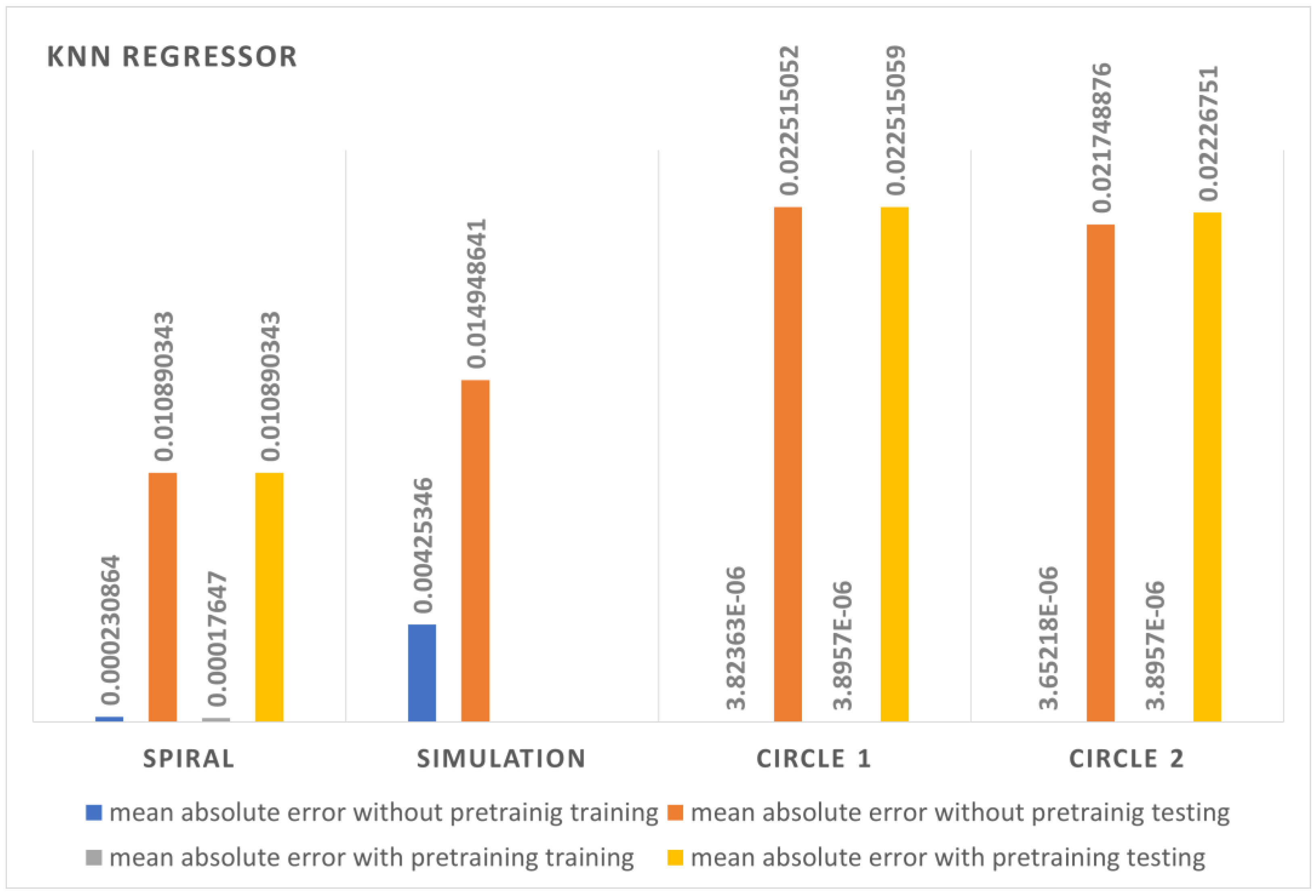
Errors from the KNN regression were comparatively less than those from all the other compared algorithms, and the batch learning method also resulted in low errors. The training errors or the real-time prediction errors varied within a few micrometers. Figure 11 shows the error comparison between the different datasets with pre-training and without pre-training. Table 2 describes the errors of the K-nearest neighbors algorithm in different databases.

Prediction errors with the unseen data led to slightly more errors since the model was generalized to the training dataset and previously learned knowledge was forgotten. The training errors were lower in the circular2 dataset both with and without pre-training. The spiral dataset had fewer testing errors compared with all the other datasets both with and without pre-training. The algorithm outperformed all the other algorithms, but it was observed that KNN was more general for the training dataset than for the unseen test data.

4.3. Decision Tree Test

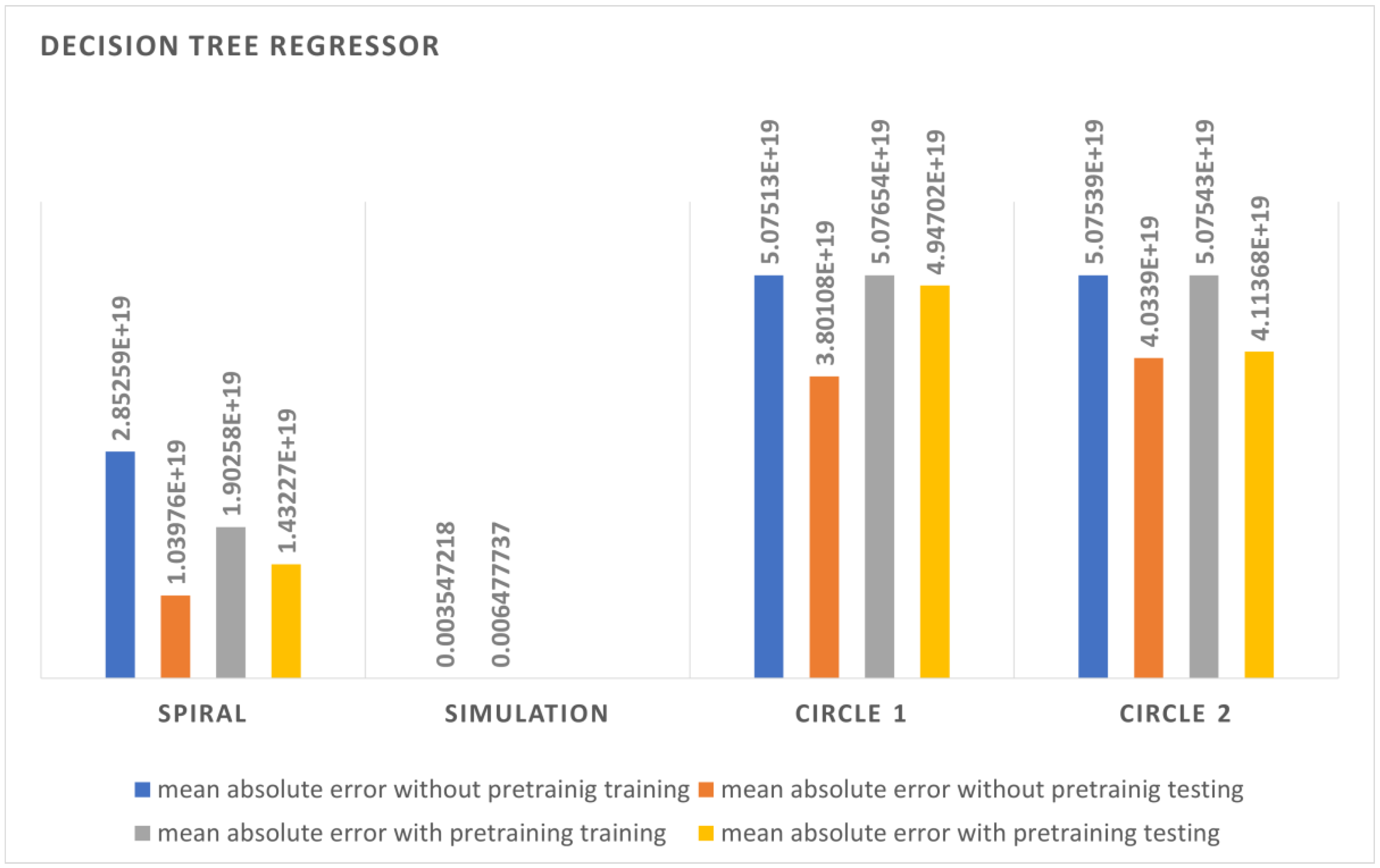
The DT algorithm showed poor performance in the incremental learning method as it had high error rates compared with all the other algorithms. The training time was also more compared with the other algorithms. The training errors were also high, and the model was not generalizable to the data. The spiral data showed an average performance using the DT algorithm, but the simulation data showed a better output compared with all the other techniques since the data were randomly picked from the workspace. The errors shown in Figure 12 could be because the model was not learning due to high error figures and because for every example that arrives, the DT model requires the construction of the model again. Hence, if the data do not reflect the structure of the tree, they will cause failure.

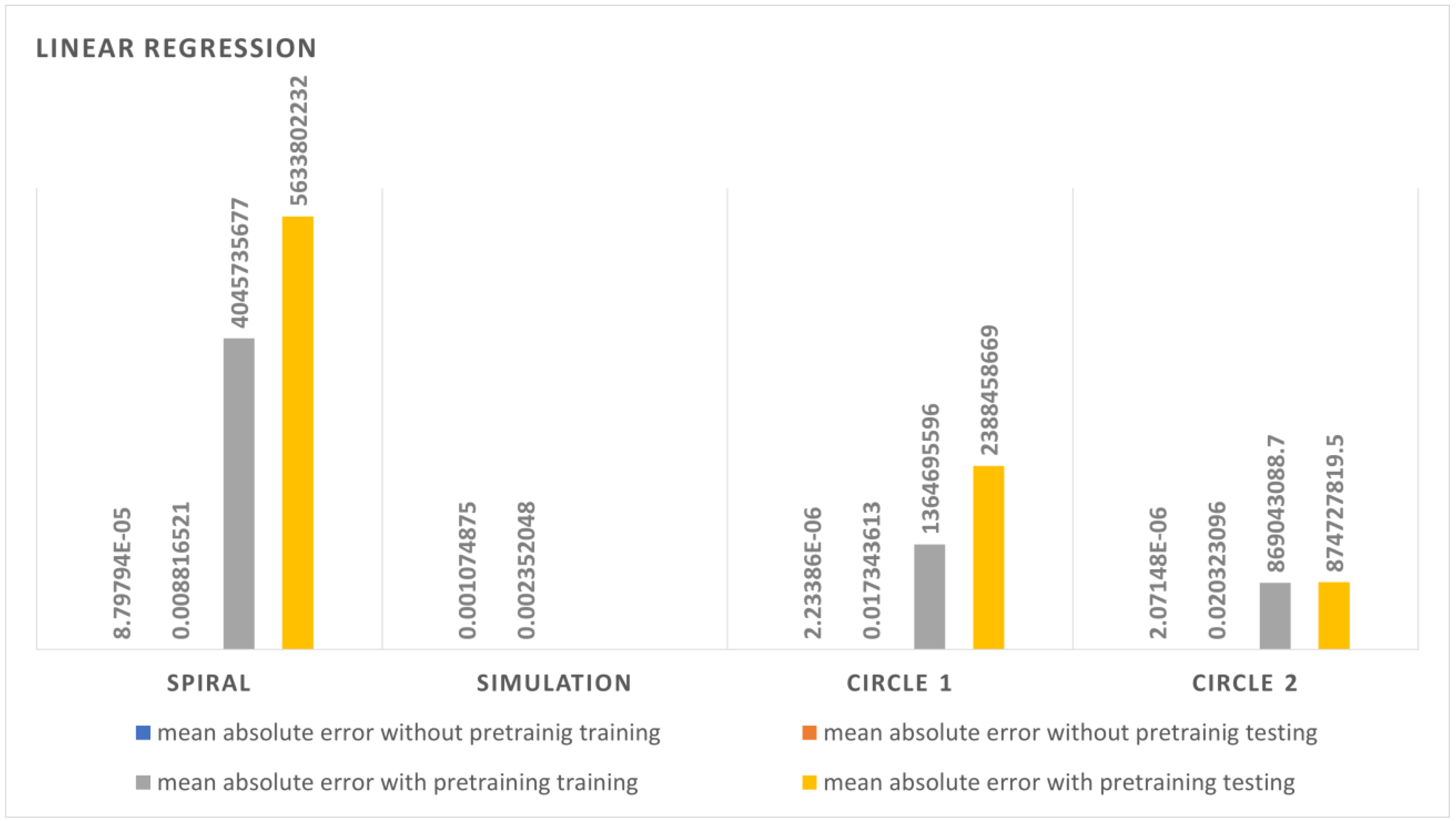
4.4. Linear Regression Test

The linear regression test demonstrated an average performance compared with the KNN regression and neural network algorithms. The error rates were between those of the DT regressor and the neural network. The simulation dataset showed fewer errors compared with the others. This is because of the randomness of the data. The spiral data also showed an average output compared with the circular dataset, which showed a good result. The pre-trained model behaved worse compared with the model with normal from-scratch training. Figure 13 shows the error comparisons of the linear regression between different datasets with and without pre-training. Transfer learning was not effective as a KNN regressor but instead deflected from the actual end-effector motion. The simulation data output obtained fewer errors compared with every other algorithm. The circular datasets resulted in more errors despite containing more data points.

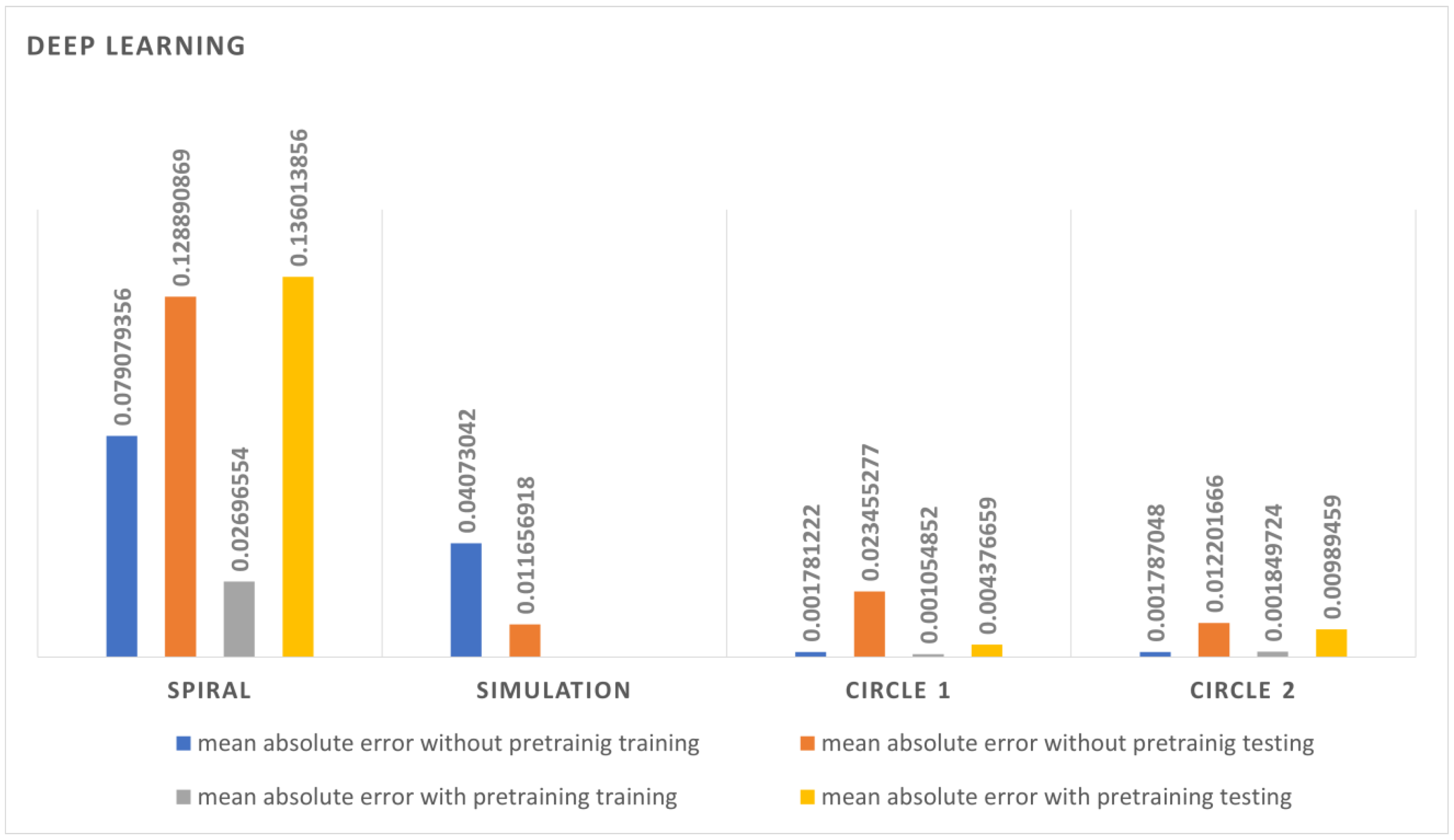
4.5. Deep Neural Network Test

The neural network performed well, but the error rate was reduced compared with the DT and LR methods. The training was performed with all the datasets the neural network depicted because it needs more datasets to learn compared with other algorithms. As can be seen in Figure 14, the error rate for the spiral dataset was higher since there were less data to learn, and it decreased as it moved toward the circular 2 dataset. The network was more generalized toward the training dataset. The neural network performed better with both circular datasets since it had an ample amount of data to learn. The pre-training had more influence on the neural network and showed fewer errors. Overall, the neural network demonstrated that it could adapt itself to changes in the data stream because each weight in neural networks is adapted to each new experience, and the weights are also dependent on the error function. This makes it comparatively easy for the neural network to update the weights.

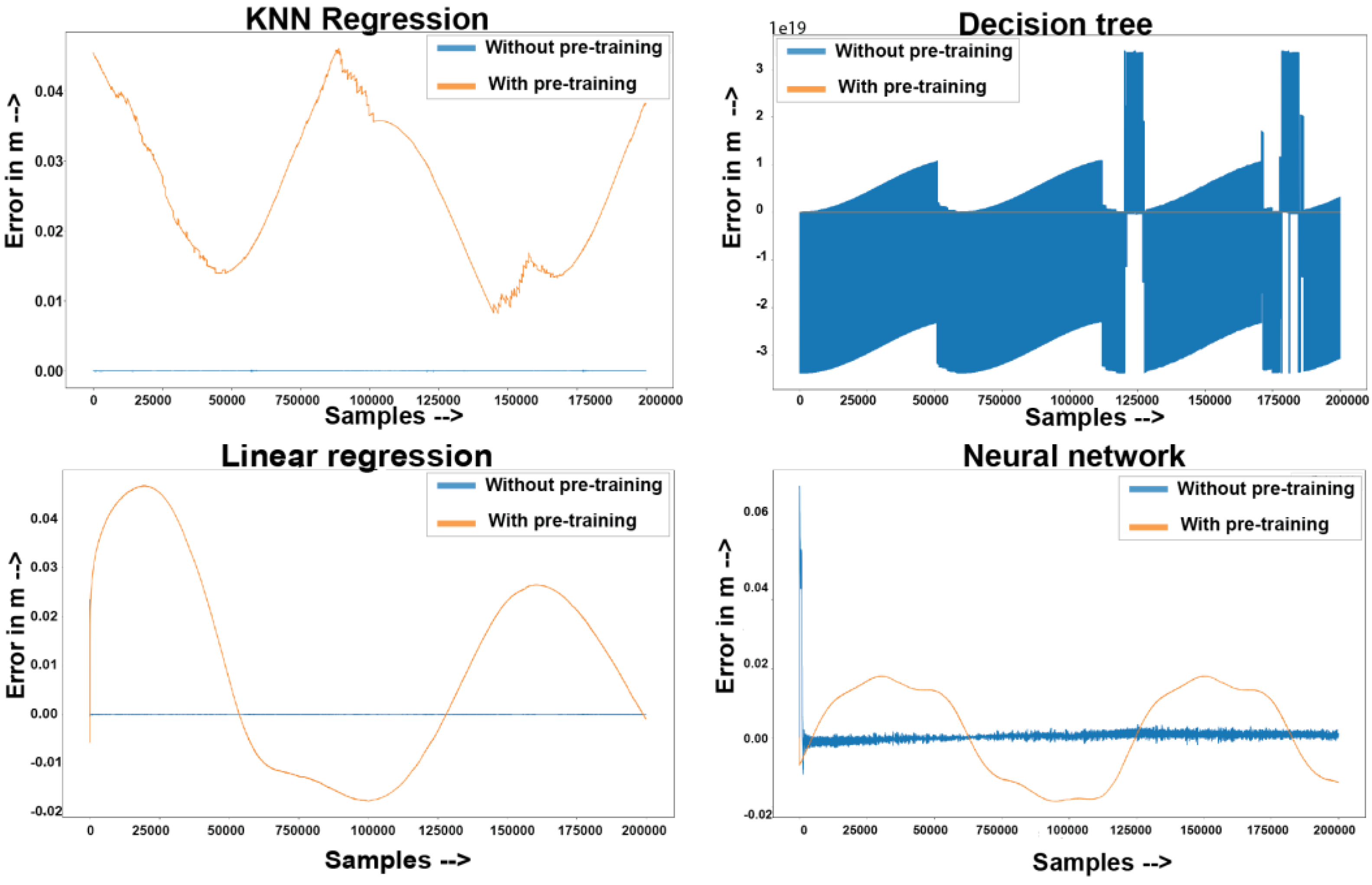
4.6. Pre-Training Effect on Error Rate

Training the neural network from scratch proved to be inefficient in the ML algorithms and good in the deep learning method, as can be deduced from the above section. The error chart depicts the average error rate at the end of model training. Transfer learning proved to reduce the error rate of the artificial neural network [15]. Figure 15 shows the error rates during the training of all the models.

The errors without pre-training showed a decreasing rate, except for DT, wherein the model in incremental learning tried to update the weights more frequently than the batch method. The transfer learning method showed a decreasing error rate in a sinusoidal fashion. This was due to the already generalized pre-trained weights and the certain workspace with different end-effector motions. The initial errors in KNN and LR were high since they used the stochastic gradient descent method to update the weights, which converged faster; hence, the models tried to merge faster and tended to build negative errors, and this continued, whereby both KNN and LR showed a decrease in the error rate for consecutive peaks and tried to converge. The neural network without pre-training tried to converge with an initially high error. The neural network with pre-training showed a decrease in error compared with all the other algorithms. This happened because transfer learning is most effective in neural networks, which use gradient descent algorithms. Gradient descent updated the weights of the network after each epoch, but with the initial pre-trained weights, the model tended to converge slower compared with the random weights, and sometimes the model never converged. The DT showed a positive response to pre-training, but the error rate without pre-training was high. Overall, transfer learning had a negative effect on incremental learning with KNN and LR. However, the neural network showed promise in reducing the initial error, but the model found it difficult to converge.

5. Conclusions and Future Work

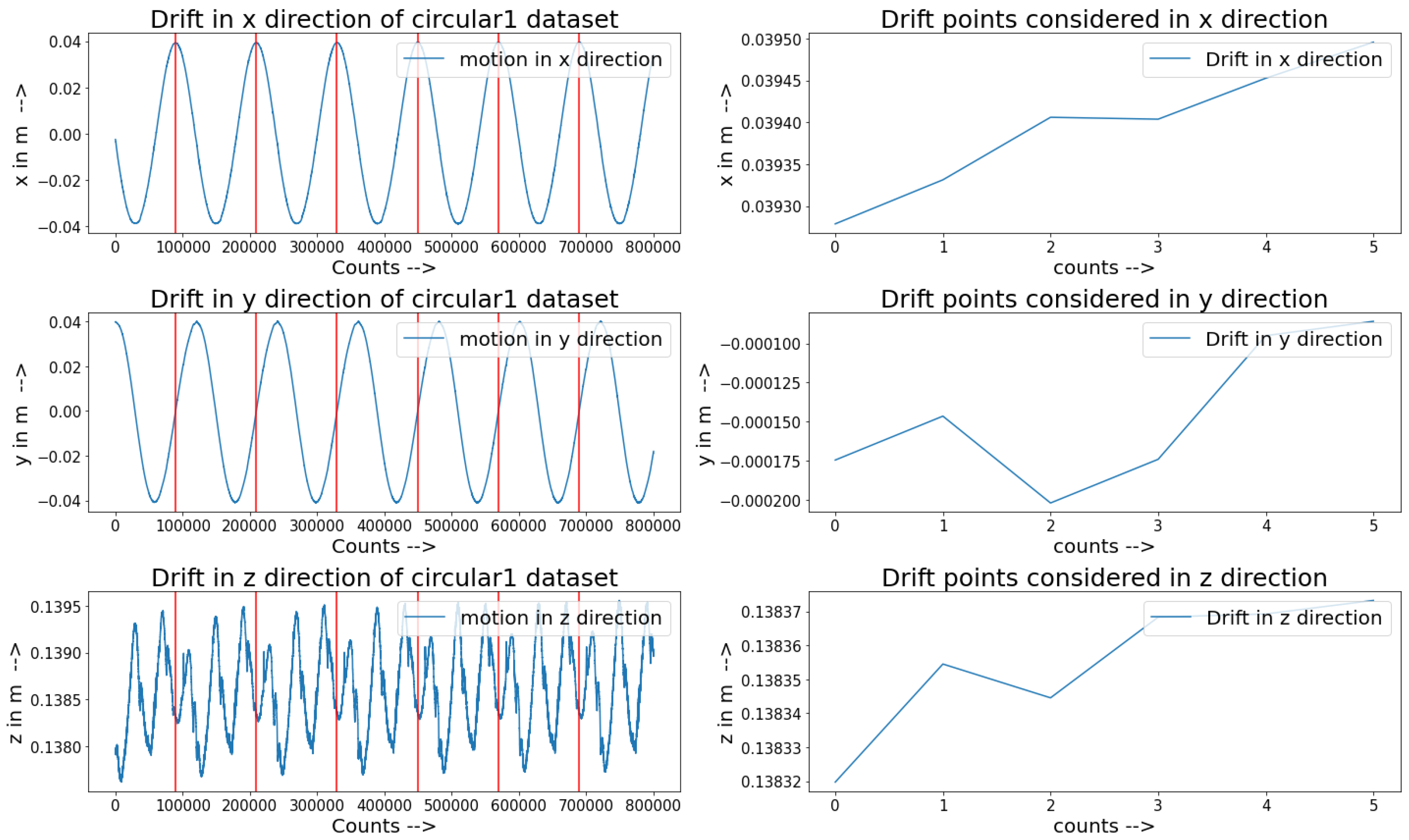
In this experiment, drift detection in streaming data and four incremental learning models for a soft pneumatic actuator were tested to predict the motion of the end-effector, with pressure as input and real-time coordinates as output. Drift was found while comparing the end-effector motions and considering certain pressure points from the input pressures. Two types of tests were initially conducted without pre-training the models and then with pre-training, and the training and testing errors were also calculated between the label and output from the models. Among all the algorithms, the KNN regressor performed best with a lower error rate for training and testing. The neural network model also performed better than the DT and LR with transferring and learning. The model was not generalized for the training data, and the testing errors of the neural network compared with those of the other low-performing algorithms were good. The decision tree regressor showed a deviation from normal behavior with significant errors in training and testing. The linear regression algorithm performed well in training, but its generalizability to the training dataset was wider, so more testing errors were obtained. Overall, the KNN regressor outperformed all the other algorithms, albeit there was a larger difference in the testing errors compared with pre-training. The neural network testing errors were fewer and were due to trying to retain the already learned knowledge.

Drift was found in the end-effector motion of the actuator, and more work should be conducted on drift detection techniques to detect types of drift. KNN and the neural network performed outstandingly with regard to testing errors, but since KNN performed poorly on the unseen test data due to forgetting, future work should be carried out considering the neural network with a new environment that is suitable for incremental learning.