Simulation Techniques for Strength Component Partially Accelerated to Analyze Stress–Strength Model

Abstract

Based on independent progressive type-II censored samples from two-parameter Burr-type XII distributions, various point and interval estimators of $\delta =P(Y<X)$ were proposed when the strength variable was subjected to the step–stress partially accelerated life test. The point estimators computed were maximum likelihood and Bayesian under various symmetric and asymmetric loss functions. The interval estimations constructed were approximate, bootstrap-P, and bootstrap-T confidence intervals, and a Bayesian credible interval. A Markov Chain Monte Carlo approach using Gibbs sampling was designed to derive the Bayesian estimate of $\delta$. Based on the mean square error, bias, confidence interval length, and coverage probability, the results of the numerical analysis of the performance of the maximum likelihood and Bayesian estimates using Monte Carlo simulations were quite satisfactory. To support the theoretical component, an empirical investigation based on two actual data sets was carried out.

1. Introduction

Stress–strength models are used in critical tasks in many fields, including engineering, mechanics, computer science, and quality control. Birnbaum [1] proposed the stress–strength concept, which Birnbaum and McCarty [2] expanded on. The reliability of a component or system $\delta$ with strength X subjected to random stress Y can be defined as the probability of the strength exceeding the stress, i.e., $X>Y$. The estimation of a component’s reliability characteristics is critical in this setup. This aids in evaluating the efficiency of a product’s operation process and allows us to take precautions to avoid interruptions in the production process. A lot of work has been carried out in recent years related to the problem of estimating $\delta$ with different sampling schemes and distributions for $(X,Y)$. Krishna et al. [3] studied the maximum likelihood (ML) and Bayesian estimation of $\delta$ under the assumption that the stress and strength variables followed a generalized inverted exponential distribution. The estimation of $\delta$, when the distribution was inverted gamma, was considered by Iranmanesh [4]. Çetinkaya and Genç [5] studied the ML and Bayesian estimation of $\delta$ under the assumption that the stress and strength variables followed a standard two-sided power distribution. Considering an exponentiated Fréchet distribution, the ML and Bayesian estimation for $\delta$ based on a type-II censoring scheme (CS) was studied by Nadeb et al. [6]. The topic of estimating $\delta$ for various distributions has been the subject of numerous publications in recent years; see, for instance, [7,8,9,10,11]. A comprehensive review can be found in Kotz et al. [12].

Modern technology has led to an increase in product reliability, which makes it difficult to evaluate items under real-life conditions and increases the cost of collecting adequate data about product lifetime. The most practical approach to solving this issue is to use accelerated life tests (ALT), in which test units are put under various levels of stress, rather than using stress to accelerate failures. The ALT is used to gather sufficient failure data in a shorter amount of time and to discuss the impact of lifetime and external stress variables. Either the acceleration factor is a known value in the case of ALT, or there is a known mathematical model that explains the relationship between lifetime and stress conditions. However, in some cases, such a life–stress relationship is unknown and cannot be assumed. As a result, in such instances, partially accelerated life tests (PALTs) are a suitable criterion for performing life tests to estimate the acceleration factor and life distribution parameters. PALT experiments are carried out under various use and stress settings, such as constant and step–stress partial ALTs. In a constant-stress PALT (CSPALT), each unit is operated at constant stress, under either normal use conditions or accelerated conditions (see [13,14,15,16,17,18,19]). On the other hand, in step–stress PALT (SSPALT), a product or system is initially exposed to normal (use) conditions for a specified period of time, and, if it survives, it is subsequently put into service at accelerated conditions until the experiment ends. SSPALT was studied in the literature by several authors. Akgul et al. [20] examined classical and Bayesian estimations of SSPALT for the inverse Weibull lifetime distribution based on type-I censoring. Based on the generalized progressive hybrid CS, Pandey et al. [21] discussed the estimation procedure for SSPALT. Pathak et al. [22] considered the estimation problem in SSPALT of Maxwell–Boltzmann distribution in the presence of progressive type-II censoring with binomial removals. In the presence of competition, the reliability of high-reliability and long-lifetime product risks were proposed by Zhang et al. [23].

Bhattacharyya and Soejoeti [24] were the first to investigate such an approach, called a tampering failure rate model (TFR), in SSPALT, where the change in stress level has a multiplicative effect on the subsequent hazard rate, i.e., $H_2\left(t\right)=\lambda H_1\left(t\right)$, $t>0$, $\lambda >0$, where $\lambda$ is the acceleration factor. This leads to

$$\begin{array}{ccc}\hfill F\left(t\right)& =& \left\{\begin{array}{c}{F}_1\left(t\right),t\le \tau \hfill \\ F_2\left(t\right)=1-{(1-F_1(\tau ))}^{1-\lambda }{(1-F_1\left(t\right))}^{\lambda },t>\tau \hfill \end{array}\right.\hfill \end{array}$$

where $F_1\left(t\right)=1-exp\{-{\int }_0^t{H}_1\left(x\right)dx\}$, $t\le \tau$.

In many reliability and life-testing studies, the observed failure time data of items are commonly not completely available. In statistical tests involving censored data, reducing the cost and time involved is crucial. Progressive censoring is one of the censoring techniques that has gained a lot of traction in studies on reliability and life testing. For more information on this censoring scheme, see Balakrishnan and Aggarwala [25]. A brief overview of this censoring scheme is given as follows. We assume the experimenters used N units of each item in the life test. We remove $r_1$ units from the remaining $N-1$ surviving units once the first failure time $X_1$ is collected. When we collect the second failure time $X_2$, we remove $r_2$ units from the remaining $N-2-r_1$ surviving units. We repeat this procedure until the nth failure time $X_n$ is collected and the experiment ends. The remaining $r_n=N-r_1-\dots -r_{n-1}-n$ units are removed automatically. We then have collected a progressive type-II censored sample given by $X_1<X_2<\dots <X_n$ under the progressive censoring scheme of $(r_1,\dots ,r_n)$.

The Burr-type XII distribution was initially described in the literature in 1942, and in the last 20 years or so, it has drawn a lot of interest because of its numerous applications in areas such as reliability, failure time modeling, acceptability sampling plans, and other areas. For instance, see Wingo [26,27], Moore [28], Wu et al. [29], Al-Saiari et al. [30], Kumar [31], and Ibrahim et al. [32]. Based on acceleration life testing applications, more papers have discussed using Burr-type XII distribution; Abd-Elfattah et al. [33] used SSPALT with type-I censoring, Rahman et al. [34] used SSPALT under type-I progressive hybrid censored data, Wang et al. [35] discussed CSPALT with competing risks under progressively type-I interval censoring, and so on.

The novelty of this study is the application of the SSPALT to units with lifetime at use condition stress assumed to follow a Burr-type XII distribution for estimating stress–strength model on progressive type-II censored data. Some inferences, such as ML estimates (MLEs), Bayesian estimates (BEs), and confidence intervals (CIs), are explored for the model parameters under consideration.

The paper is drafted as follows: Section 2 presents a description of the lifetime model and the explicit expression of $\delta$. The MLE of $\delta$ under SSPALT is derived in Section 3. In Section 4, we calculate the BEs of $\delta$ under the squared error (SE), linear exponential error (LINEX), and general entropy (GE) loss functions using the Markov Chain Monte Carlo (MCMC) approach. Various interval estimates of $\delta$ are presented in Section 5, including approximate, bootstrap-P, and bootstrap-T confidence intervals (CIs), and Bayesian credible interval. An intense simulation technique with various CSs to compare the performance of estimation methods is employed in Section 6. In Section 7, we examine two real data sets, to demonstrate the suggested techniques. Finally, we present conclusions and future scope in Section 8.

2. Model Assumptions and Description

In this section, the reliability $\delta$ was derived, where the random variables X and Y were the independent random variables, of which X denotes the total lifetime of a test item, such as strength, under SSPALT. The details of the model are introduced, and the parameters of independent Burr-type XII failure causes and acceleration factor in SSPALT with progressive type-II censoring are also denoted.

(1) The failure data under normal stress $S_0$ was modeled by Burr-type XII distribution, which has the below hazard rate function (HRF) and reliability function (RF), respectively, expressed as follows:

$$\left.\begin{array}{cc}\hfill H_1(x;\alpha ,{\beta }_1)& =\frac{\alpha {\beta }_1{x}^{\alpha -1}}{(1+x^{\alpha })},x>0,\hfill \\ \hfill {\overline{F}}_1(x;\alpha ,{\beta }_1)& ={(1+x^{\alpha })}^{-{\beta }_1}.\hfill \end{array}\right\}$$

(1)

(2) Based on the TFR model, the effect of switching the stress $S_0$ to the stress $S_1$ at $\tau$ is obtained by multiplying the $H_1(x;\alpha ,{\beta }_1)$ by an acceleration factor $\lambda \ge 1$. Then, the $H_2(x;\alpha ,{\beta }_1,\lambda )$ is given as shown:

$$\begin{array}{cc}\hfill H_2(x;\alpha ,{\beta }_1,\lambda )& =\frac{\alpha {\beta }_1\lambda x^{\alpha -1}}{(1+x^{\alpha })},x>0\hfill \end{array}$$

(2)

and the RF is as follows:

$$\begin{array}{cc}\hfill {\overline{F}}_2(x;\alpha ,{\beta }_1,\lambda )& ={(1+{\tau }^{\alpha })}^{-{\beta }_1(1-\lambda )}{(1+x^{\alpha })}^{-{\beta }_1\lambda },x>0\hfill \end{array}$$

(3)

(3) We let strength X, under SSPALT with the probability density function (PDF) $f(.)$ and the cumulative distribution function (CDF) $F(.)$, and primary stress Y, with PDF $g(.)$ and CDF $G(.)$, be two independent random variables from Burr $(\alpha ,{\beta }_1)$ and Burr $(\alpha ,{\beta }_2)$, respectively. Additionally, $\alpha$ was used as a known common shape parameter. Çetinkaya [36] assumed that partially accelerated life test-implemented stress–strength reliability estimation could be derived as follows:

$$\begin{array}{cc}\hfill \delta =P(X>Y)& ={\int }_0^{\tau }{\int }_0^x{f}_1\left(x\right)dG\left(y\right)dx+{\int }_{\tau }^{\infty }{\int }_0^x{f}_2\left(x\right)dG\left(y\right)dx.\hfill \end{array}$$

(4)

According to Bhattacharyya and Soejoeti [24], the PDF of SSPALT implemented strength variable X is given by the following:

$$\begin{array}{ccc}\hfill f(x;\alpha ,{\beta }_1,\lambda )& =& \left\{\begin{array}{c}{f}_1\left(x\right)=\alpha {\beta }_1{x}^{\alpha -1}{(1+x^{\alpha })}^{-({\beta }_1+1)},x\le \tau ,\hfill \\ f_2\left(x\right)=\alpha {\beta }_1\lambda x^{\alpha -1}{(1+x^{\alpha })}^{-({\beta }_1\lambda +1)}{(1+{\tau }^{\alpha })}^{-{\beta }_1(1-\lambda )},x>\tau .\hfill \end{array}\right.\hfill \end{array}$$

(5)

The PDF and the CDF of primary stress Y are given as shown:

$$\left.\begin{array}{cc}\hfill g(y;\alpha ,{\beta }_2)& =\alpha {\beta }_2{y}^{\alpha -1}{(1+y^{\alpha })}^{-({\beta }_2+1)},y>0,\hfill \\ \hfill G(y;\alpha ,{\beta }_2)& =1-{(1+y^{\alpha })}^{-{\beta }_2}.\hfill \end{array}\right\}$$

(6)

Thus, using (5) and (6), the conventional reliability model $\delta$ can be expressed:

$$\begin{array}{c}\hfill \delta =\frac{{\beta }_2}{{\beta }_1+{\beta }_2}\left[1+\frac{1-\lambda }{\lambda +{\beta }_2/{\beta }_1}{(1+{\tau }^{\alpha })}^{-({\beta }_1+{\beta }_2)}\right].\end{array}$$

(7)

Note that the reliability $\delta$ depends on the parameters ${\beta }_1$ and ${\beta }_2$ (see Figure 1).

Figure 1 shows the 3D plot of the reliability stress–strength model with different values of ${\beta }_1$ and ${\beta }_2$. These figures indicate that the reliability stress–strength model increases.

We can see that for Burr-type XII distributed stress and strength components (without any acceleration), (7) equals the reliability for a simple stress–strength system when $\lambda =1$.

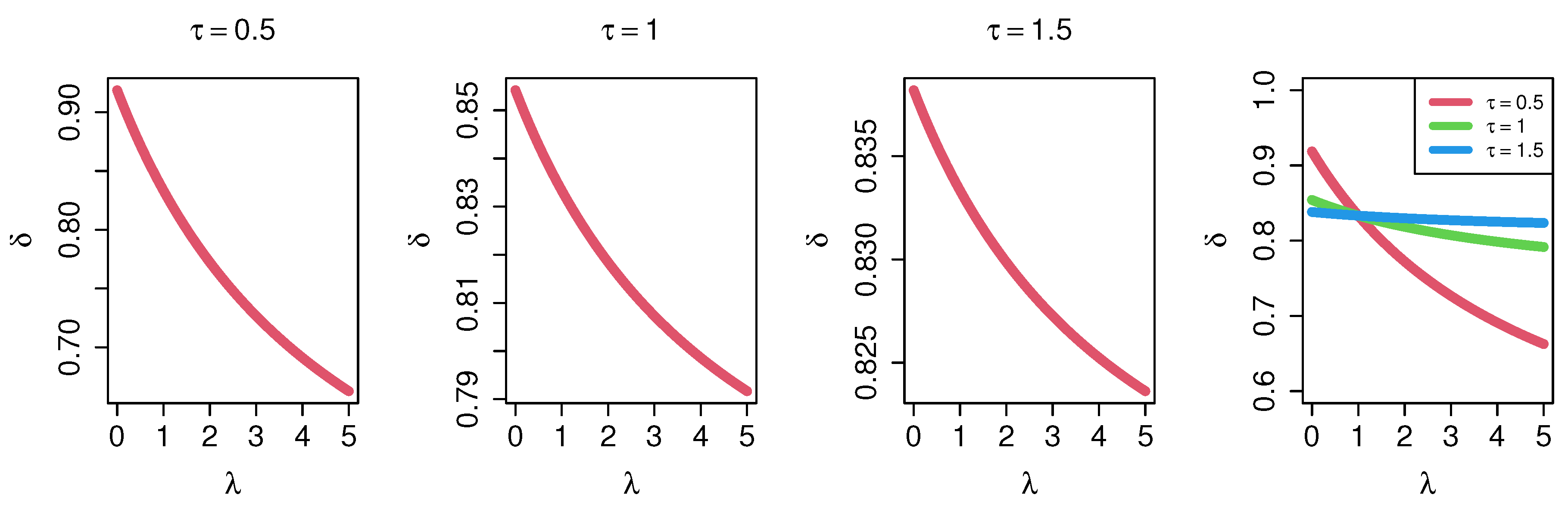
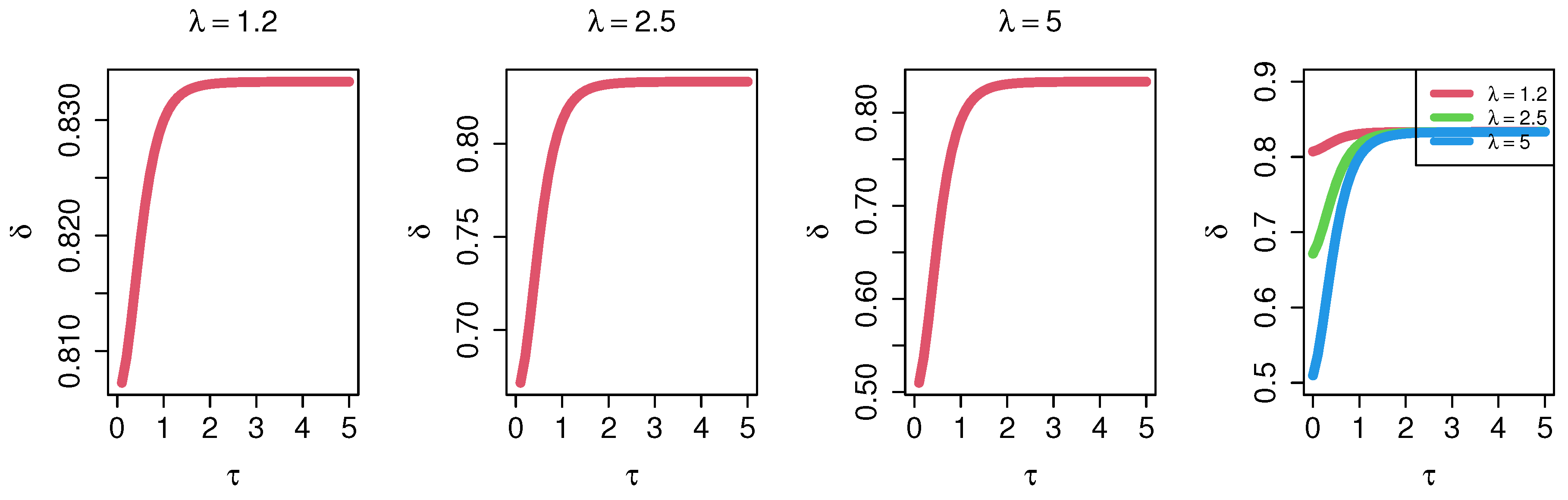
We notice that, in this reliability scheme, the system’s reliability increases when the stress change time $\tau$ increases, even when the acceleration factor $\lambda$ is greater than 1, as in Figure 2. Moreover, increasing the acceleration factor $\lambda$ quickly decreases reliability, as shown in Figure 3.

3. Maximum Likelihood Estimation of $\mathbf{\delta }$

In this section, we suppose $x_{1:n:N},\dots ,x_{n:n:N}$ to be a progressively censored sample of strength, and $y_{1:m:M},\dots ,y_{m:m:M}$ to be a progressively censored sample of primary stress, under the schemes $(N,n,r_1,r_2,\dots ,r_n)$ and $(M,m,s_1,s_2,\dots ,s_m)$, respectively. Then, the likelihood function (LF) of the observed samples in this reliability scheme is given by the following:

$$\begin{array}{cc}\hfill L\left(\phi \right|\mathbf{x},\mathbf{y})& =C\prod _{i=1}^{n_u}{f}_1\left(x_i\right|\phi ){\left({\overline{F}}_1\left(x_i\right|\phi )\right)}^{r_i}\prod _{i=n_u+1}^n{f}_2\left(x_i\right|\phi ){\left({\overline{F}}_2\left(x_i\right|\phi )\right)}^{r_i}\prod _{i=1}^{m}g\left(y_i\right|\phi ){\left(\overline{G}\left(y_i\right|\phi )\right)}^{s_i},\hfill \end{array}$$

where

$$\begin{array}{cc}\hfill C& =c_1{c}_2,\hfill \\ \hfill c_1& =N(N-r_1-1)\dots (N-r_1-\dots -r_{n-1}-n+1),\hfill \\ \hfill c_2& =M(M-s_1-1)\dots (M-s_1-\dots -s_{m-1}-m+1).\hfill \end{array}$$

and $\phi =(\alpha ,{\beta }_1,{\beta }_2)$ is a set of parameters and $x_i=x_{i:n:N}$ to simplify the notation. Based on the observed data, the LF, according to Çetinkaya [36], is given as follows:

$$\begin{array}{cc}\hfill L\left(\phi \right|\mathbf{x},\mathbf{y})& =C{\alpha }^{n+m}{\beta }_1^n{\beta }_2^m{\lambda }^{n-n_u}\prod _{i=1}^{n_u}{x}_i^{\alpha -1}{(1+x_i^{\alpha })}^{-({\beta }_1(r_i+1)+1)}\prod _{i=n_u+1}^n{x}_i^{\alpha -1}{(1+x_i^{\alpha })}^{-({\beta }_1\lambda (r_i+1)+1)}\hfill \\ \hfill & \times {(1+{\tau }^{\alpha })}^{-{\beta }_1(1-\lambda )(r_i+1)}\prod _{i=1}^m{y}_i^{\alpha -1}{(1+y_i^{\alpha })}^{-({\beta }_2(s_i+1)+1)}.\hfill \end{array}$$

(8)

and $x_1^r<\dots <x_{n_u}^r<\tau <x_{n_u+1}^r<\dots <x_n^r$. Then, the natural logarithm of the LF (8) is reduced to the following:

$$\begin{array}{cc}\hfill l\left(\phi \right|\mathbf{x},\mathbf{y})& \propto (n+m)ln\alpha +nln{\beta }_1+mln{\beta }_2+(n-n_u)ln\lambda +(\alpha -1)[\sum _{i=1}^{n_u}ln{x}_i\hfill \\ \hfill & +\sum _{i=n_u+1}^{n}ln{x}_i+\sum _{i=1}^{m}ln{y}_i]-\sum _{i=1}^{n_u}{\psi }_1({\beta }_1,r_i)ln(1+x_i^{\alpha })-\sum _{i=n_u+1}^n{\psi }_2({\beta }_1,\lambda ,r_i)ln(1+x_i^{\alpha })\hfill \\ \hfill & -\sum _{i=n_u+1}^n({\psi }_1({\beta }_1,r_i)-{\psi }_2({\beta }_1,\lambda ,r_i))ln(1+{\tau }^{\alpha })-\sum _{i=1}^m{\psi }_3({\beta }_2,s_i)ln(1+y_i^{\alpha }),\hfill \end{array}$$

(9)

where

$$\begin{array}{c}\hfill {\psi }_2({\beta }_1,\lambda ,r_i)={\beta }_1\lambda (r_i+1)+1.\end{array}$$

(10)

and ${\psi }_1({\beta }_1,r_i)$, ${\psi }_3({\beta }_2,s_i)$ are the same as in (10), with $\lambda =1$ and ${\beta }_2,s_i$ replaced by ${\beta }_1,r_i$. Moreover, $\alpha$ is a known common shape parameter. The log LF $l\left(\phi \right|\mathbf{x},\mathbf{y})$ can be maximized directly for parameter vector $\phi ({\beta }_1,{\beta }_2,\lambda )$ to obtain MLEs of ${\beta }_1,{\beta }_2$, and $\lambda$. Differentiating (9) with respect to ${\beta }_1,{\beta }_2$, and $\lambda$, respectively, and equating to zero leads to the following:

$$\left.\begin{array}{cc}\hfill \frac{\partial l\left(\phi \right|\mathbf{x},\mathbf{y})}{\partial {\beta }_1}& =\frac{n}{{\beta }_1}-\sum _{i=1}^{n_u}(r_i+1)ln(1+x_i^{\alpha })-\sum _{i=n_u+1}^n\lambda (r_i+1)ln(1+x_i^{\alpha })\hfill \\ \hfill & -\sum _{i=n_u+1}^n(1-\lambda )(r_i+1)ln(1+{\tau }^{\alpha }),\hfill \\ \hfill \frac{\partial l\left(\phi \right|\mathbf{x},\mathbf{y})}{\partial {\beta }_2}& =\frac{m}{{\beta }_2}-\sum _{i=1}^m(s_i+1)ln(1+y_i^{\alpha }),\hfill \\ \hfill \frac{\partial l\left(\phi \right|\mathbf{x},\mathbf{y})}{\partial \lambda }& =\frac{n-n_u}{\lambda }-\sum _{i=n_u+1}^n{\beta }_1(r_i+1)ln(1+x_i^{\alpha })+\sum _{i=n_u+1}^n{\beta }_1(r_i+1)ln(1+{\tau }^{\alpha }).\hfill \end{array}\right\}$$

(11)

Then, the derivatives with respect to ${\beta }_1,{\beta }_2$, and $\lambda$ are reduced to the following:

$$\begin{array}{cc}\hfill & {\widehat{\beta }}_1=n/\left[\sum _{i=1}^{n_u}(r_i+1)ln(1+x_i^{\alpha })+\sum _{i=n_u+1}^n\lambda (r_i+1)ln(1+x_i^{\alpha })+\sum _{i=n_u+1}^n(1-\lambda )(r_i+1)ln(1+{\tau }^{\alpha })\right],\hfill \\ & {\widehat{\beta }}_2=m/\left[\sum _{i=1}^m(s_i+1)ln(1+y_i^{\alpha })\right],\hfill \\ & \widehat{\lambda }=(n-n_u)/\left[\sum _{i=n_u+1}^n{\beta }_1(r_i+1)ln(1+x_i^{\alpha })-\sum _{i=n_u+1}^n{\beta }_1(r_i+1)ln(1+{\tau }^{\alpha })\right].\hfill \end{array}$$

Replacing ${\beta }_1,{\beta }_2$, and $\lambda$ with their estimates ${\widehat{\beta }}_1,{\widehat{\beta }}_2$, and $\widehat{\lambda }$, respectively, in (7), the MLE of $\delta$, denoted by ${\widehat{\delta }}_{ML}$, becomes the following:

$$\begin{array}{c}\hfill {\widehat{\delta }}_{ML}=\frac{{\widehat{\beta }}_2}{{\widehat{\beta }}_1+{\widehat{\beta }}_2}\left[1+\frac{1-\widehat{\lambda }}{\widehat{\lambda }+{\widehat{\beta }}_2/{\widehat{\beta }}_1}{(1+{\tau }^{\alpha })}^{-({\widehat{\beta }}_1+{\widehat{\beta }}_2)}\right].\end{array}$$

(12)

4. Bayesian Analysis of $\mathbf{\delta }$

In this section, we focus on the Bayesian estimate of $\delta$ with a common and known shape parameter $\alpha$. We utilized the Bayesian estimation to estimate $\delta$ under various loss functions. The point estimators $\tilde{\phi }$ were derived from the sample data’s posterior distributions. The estimator that could minimize the SE loss function for the given prior distribution was ${(\tilde{\phi }-\phi )}^2$, which was the posterior mean; in this case, ${\tilde{\delta }}_{SE}=\frac{1}{A-B}{\sum }_{i=B+1}^A{\delta }^{\left(i\right)}$ was computed. The LINEX loss function with parameters $\epsilon$ was described by $(e^{\epsilon (\tilde{\phi }-\phi )}-\epsilon (\tilde{\phi }-\phi )-1)$, and it was minimized by ${\tilde{\delta }}_{LN}=\frac{-1}{\epsilon }[log\frac{1}{A-B}{\sum }_{i=B+1}^A{e}^{-\epsilon {\delta }^{\left(i\right)}}]$, where the sign of the parameter $\epsilon$ represented the direction of asymmetry, whereas the value indicated the degree of asymmetry. The GE loss function was defined as ${\left(\frac{\tilde{\phi }}{\phi }\right)}^{\gamma }-\gamma \left(\frac{\tilde{\phi }}{\phi }\right)-1$, and we minimized it by ${\tilde{\delta }}_{GE}={\left[\frac{1}{A-B}{\sum }_{i=B+1}^A{\left({\delta }^{\left(i\right)}\right)}^{-\gamma }\right]}^{\frac{-1}{\gamma }}$. A was the number of iterations and B was the burn-in. More papers discussed Bayesian estimation based on different loss functions, such as [37,38], and so on.

We assumed, in the Bayesian framework, that the parameters ${\beta }_1,{\beta }_2$, and $\lambda$ were independently distributed according to a gamma distribution and a non-informative prior (NIP) distribution. The joint prior distribution of $({\beta }_1,{\beta }_2,\lambda )$ was then given by the following:

$$\begin{array}{c}\hfill P({\beta }_1,{\beta }_2,\lambda )=\frac{{\beta }_1^{a_1-1}{\beta }_2^{a_2-1}{\lambda }^{-1}}{\Gamma \left(a_1\right)\Gamma \left(a_2\right)b_1^{a_1}{b}_2^{a_2}}{e}^{-(\frac{{\beta }_1}{b_1}+\frac{{\beta }_2}{b_2})}.\end{array}$$

(13)

Based on the observed sample $(\mathbf{x},\mathbf{y})$, the joint posterior distribution of ${\beta }_1,{\beta }_2$, and $\lambda$ could be written as shown:

$$\begin{array}{cc}\hfill P^{*}({\beta }_1,{\beta }_2,\lambda |\mathbf{x},\mathbf{y})& \propto {\alpha }^{n+m}{\beta }_1^{n+a_1-1}{\beta }_2^{m+a_2-1}{\lambda }^{n-n_u-1}{e}^{-(\frac{{\beta }_1}{b_1}+\frac{{\beta }_2}{b_2})}\hfill \\ \hfill & \times \prod _{i=1}^{n_u}{x}_i^{\alpha -1}{(1+x_i^{\alpha })}^{-({\beta }_1(r_i+1)+1)}\prod _{i=n_u+1}^n{x}_i^{\alpha -1}{(1+x_i^{\alpha })}^{-({\beta }_1\lambda (r_i+1)+1)}\hfill \\ \hfill & \times {(1+{\tau }^{\alpha })}^{-{\beta }_1(1-\lambda )(r_i+1)}\prod _{i=1}^m{y}_i^{\alpha -1}{(1+y_i^{\alpha })}^{-({\beta }_2(s_i+1)+1)}.\hfill \end{array}$$

(14)

Because the joint posterior distribution of ${\beta }_1,{\beta }_2$, and $\lambda$ in (14) cannot be calculated analytically, the Bayesian estimates were generated using the MCMC approach. Thus, we investigated the MCMC technique, specifically the Gibbs sampler, which is best used on problems where the marginal distributions of the parameters of interest are difficult to compute but the conditional distributions of each parameter, given all the other parameters and data, have good forms. The Gibbs sampler generated a series of samples from the full conditional probability distribution. The full posterior conditional distributions of parameters ${\beta }_1,{\beta }_2$, and $\lambda$ were defined as follows:

$$\begin{array}{cc}\hfill & P^{*}\left({\beta }_1\right|{\beta }_2,\lambda )\propto {\beta }_1^{n+a_1-1}{e}^{-{\beta }_1(\frac{1}{b_1}+{\sum }_{i=1}^{n_u}(r_i+1)ln(1+x_i^{\alpha })+{\sum }_{i=n_u+1}^n\lambda (r_i+1)ln(1+x_i^{\alpha })+{\sum }_{i=n_u+1}^n(1-\lambda )(r_i+1)ln(1+{\tau }^{\alpha }))}\hfill \\ & P^{*}\left({\beta }_2\right|{\beta }_1,\lambda )\propto {\beta }_2^{m+a_2-1}{e}^{-{\beta }_2(\frac{1}{b_2}+{\sum }_{i=1}^m(s_i+1)ln(1+y_i^{\alpha }))}\hfill \\ & P^{*}\left(\lambda \right|{\beta }_1,{\beta }_2)\propto {\lambda }^{n-n_u-1}{e}^{-\lambda \left({\sum }_{i=n_u+1}^n{\beta }_1(r_i+1)(ln(1+x_i^{\alpha })-ln(1+{\tau }^{\alpha }))\right)}\hfill \end{array}$$

The Gibbs algorithm consists of the steps listed below:

• Begin with an initial guess ${\beta }_1^{\left(0\right)},{\beta }_2^{\left(0\right)},{\lambda }^{\left(0\right)}$.
• Set $u=1$.
• Generate ${\beta }_1^{\left(u\right)}$ from $\Gamma (n+a_1,1/(\frac{1}{b_1}+{\sum }_{i=1}^{n_u}(r_i+1)ln(1+x_i^{\alpha })+{\sum }_{i=n_u+1}^n{\lambda }^{(u-1)}(r_i+1)ln(1+x_i^{\alpha })+{\sum }_{i=n_u+1}^n(1-{\lambda }^{(u-1)})(r_i+1)ln(1+{\tau }^{\alpha })))$.
• Generate ${\beta }_2^{\left(u\right)}$ from $\Gamma (m+a_2,1/(\frac{1}{b_2}+{\sum }_{i=1}^m(s_i+1)ln(1+y_i^{\alpha })))$.
• Generate ${\lambda }^{\left(u\right)}$ from $\Gamma (n-n_u,1/\left({\sum }_{i=n_u+1}^n{\beta }_1^{\left(u\right)}(r_i+1)(ln(1+x_i^{\alpha })-ln(1+{\tau }^{\alpha }))\right))$.
• compute ${\delta }^{\left(u\right)}$ at ${\beta }_1^{\left(u\right)},{\beta }_2^{\left(u\right)},{\lambda }^{\left(u\right)}$.
• Set $u=u+1$.
• Repeat steps 2 to 7 K times.

We can calculate an approximation of ${\delta }_{SE},{\delta }_{NL}$, and ${\delta }_{GE}$ for a sufficiently large value of K.

5. Confidence Intervals of $\mathbf{\delta }$

In this section, we present an asymptotic confidence interval (ACI) of $\delta$ based on the asymptotic distribution of $\widehat{\delta }$. For comparison, another two CIs based on bootstrap methods and credible interval for the Bayesian estimation method are proposed in this section.

5.1. Approximate Confidence Interval

The Fisher information matrix of $\phi ({\beta }_1,{\beta }_2,\lambda )$ is $D\left(\phi \right)=E\left(I\right(\phi \left)\right)$, where $I\left(\phi \right)={\left[Iij\right]}_{i,j=1,2,3}$ is the observed information matrix, that is,

$$I\left(\phi \right)=-\left(\frac{{\partial }^{2}l\left(\phi \right|\mathbf{x},\mathbf{y})}{\partial {\theta }_{\eta }\partial {\theta }_{\zeta }}\right){|}_{{}_{(\widehat{{\beta }_1},\widehat{{\beta }_2},\widehat{\lambda })}},\eta ,\zeta =1,2,3,{\theta }_1={\beta }_1,{\theta }_2={\beta }_2,{\theta }_3=\lambda .$$

It is easy to see that

$$\begin{array}{cc}\hfill J_{11}& =\frac{-n}{{\beta }_1^2},\hfill \\ \hfill J_{22}& =\frac{-m}{{\beta }_2^2},\hfill \\ \hfill J_{33}& =\frac{-(n-nu)}{{\lambda }^2},\hfill \\ \hfill J_{13}& =-\sum _{nu+1}^n(r_i+1)ln(1+x_i^{\alpha })+\sum _{nu+1}^n(r_i+1)ln(1+{\tau }^{\alpha }),\hfill \\ \hfill J_{12}& =J_{21}=J_{23}=J_{32}=0.\hfill \end{array}$$

By applying the delta method, $\widehat{\delta }=q(\widehat{{\beta }_1},\widehat{{\beta }_2},\widehat{\lambda })$ is asymptotic and normally distributed, with mean $\delta$ and variance:

$$\begin{array}{c}\hfill D^2={\left(\frac{\partial \delta }{\partial {\beta }_1}\right)}^2{J}_{11}^{-1}+{\left(\frac{\partial \delta }{\partial {\beta }_2}\right)}^2{J}_{22}^{-1}+{\left(\frac{\partial \delta }{\partial \lambda }\right)}^2{J}_{33}^{-1}+2\left(\frac{\partial \delta }{\partial {\beta }_1}\frac{\partial \delta }{\partial \lambda }\right)J_{13}^{-1},\end{array}$$

(15)

where

$$\begin{array}{cc}\hfill \frac{\partial \delta }{\partial {\beta }_1}& =-\frac{{\beta }_2}{{({\beta }_1+{\beta }_2)}^2}+\frac{{\beta }_2(1-\lambda ){(1+{\tau }^{\alpha })}^{-({\beta }_1+{\beta }_2)}}{({\beta }_1+{\beta }_2)(\lambda {\beta }_1+{\beta }_2)}\left(\frac{{\beta }_2^2-\lambda {\beta }_1^2}{({\beta }_1+{\beta }_2)(\lambda {\beta }_1+{\beta }_2)}-{\beta }_{1}ln(1+{\tau }^{\alpha })\right),\hfill \\ \hfill \frac{\partial \delta }{\partial {\beta }_2}& =\frac{{\beta }_1}{{({\beta }_1+{\beta }_2)}^2}+\frac{{\beta }_1(1-\lambda ){(1+{\tau }^{\alpha })}^{-({\beta }_1+{\beta }_2)}}{({\beta }_1+{\beta }_2)(\lambda {\beta }_1+{\beta }_2)}\left(\frac{\lambda {\beta }_1^2-{\beta }_2^2}{({\beta }_1+{\beta }_2)(\lambda {\beta }_1+{\beta }_2)}-{\beta }_{2}ln(1+{\tau }^{\alpha })\right),\hfill \\ \hfill \frac{\partial \delta }{\partial \lambda }& =-\frac{{\beta }_1{\beta }_2}{{(\lambda {\beta }_1+{\beta }_2)}^2}{(1+{\tau }^{\alpha })}^{-({\beta }_1+{\beta }_2)},\hfill \end{array}$$

and $J_{11}^{-1},J_{22}^{-1},J_{33}^{-1}$ and $J_{13}^{-1}$ are the ${\left(ij\right)}^{th}$ elements of the inverse of the information matrix $I\left(\phi \right)$.

As a result, a 100% ACI of $\delta$ can be created:

$$\begin{array}{c}\hfill \left(\widehat{\delta }-z_{\frac{\xi }{2}}\widehat{D},\widehat{\delta }+z_{\frac{\xi }{2}}\widehat{D}\right),\end{array}$$

(16)

where $z_{\frac{\xi }{2}}$ is the upper $\frac{\xi }{2}$ percentile of the standard normal distribution.

5.2. Bootstrap Confidence Intervals

When the sample observations are insufficiently large, the assumption of asymptotic normality of MLE may be invalid. ACIs of parameters outlined in the previous subsection may not be a good choice in such instances. Instead, we considered bootstrap CI for $\delta$ based on Efron’s [39] bootstrapping approach and gave a procedure to achieve percentile bootstrap (boot-P) CI as well as bootstrap CI based on the t statistic (boot-T).

• Boot-P

The main steps to be followed under this technique are as follows:

Step 1. From the data $(\mathbf{x},\mathbf{y})$, compute ${\widehat{\beta }}_1,{\widehat{\beta }}_2$ and $\widehat{\lambda }$, respectively.

Step 2. Generate the progressively censored sample $x_1^{*},x_2^{*},\dots ,x_n^{*}$ from $f(x;\alpha ,{\widehat{\beta }}_1,\widehat{\lambda })$ and similarly, generate the progressively censored sample $y_1^{*},y_2^{*},\dots ,y_m^{*}$ from $g(y;\alpha ,{\widehat{\beta }}_2)$.

Step 3. Examine the bootstrap estimate ${\widehat{\delta }}^{*}$ of $\delta$.

Step 4. Repeat steps 2–3, Q boot times, to get order values ${\widehat{\delta }}_1^{*},{\widehat{\delta }}_2^{*},\dots ,{\widehat{\delta }}_Q^{*}$.

Step 5. Let $U\left(x\right)=P({\widehat{\delta }}^{*}\le x)$ be the cumulative distribution function of ${\widehat{\delta }}^{*}$. Define ${\widehat{\delta }}_{BP}\left(x\right)=U^{-1}\left(x\right)$ for a given x. The approximate $100(1-\xi )\%$ CI of $\delta$ is given by the following:

$$\begin{array}{c}\hfill \left({\widehat{\delta }}_{BP}\left(\frac{\xi }{2}\right),{\widehat{\delta }}_{BP}(1-\frac{\xi }{2})\right).\end{array}$$

(17)

• Boot-T

The boot-P procedure described above is the same for steps 1 through 4.

Step 5. Calculate ${\widehat{T}}^{*}=({\widehat{\delta }}^{*}-\widehat{\delta })/\sqrt{Var\left({\widehat{\delta }}^{*}\right)}$, to get order values ${\widehat{T}}_1^{*}\le {\widehat{T}}_2^{*}\le \dots \le {\widehat{T}}_Q^{*}$.

Step 6. The cumulative distribution function of $T^{*}$ is defined as $V\left(x\right)=P(T^{*}\le x)$. For a specific x, the following is defined:

$$\begin{array}{c}\hfill {\widehat{\delta }}_{BT}\left(x\right)=\widehat{\delta }+n^{-\frac{1}{2}}{V}^{-1}\left(x\right)\sqrt{V\left(\widehat{\delta }\right)}.\end{array}$$

(18)

Then, $100(1-\xi )\%$ boot-T CI is as shown:

$$\begin{array}{c}\hfill \left({\widehat{\delta }}_{BT}\left(\frac{\xi }{2}\right),{\widehat{\delta }}_{BT}(1-\frac{\xi }{2})\right).\end{array}$$

(19)

5.3. Bayesian Credible Confidence Interval

The highest posterior density (HPD) CIs were employed to construct credible CIs of parameters of this model for the outcomes of the MCMC. According to Chen and Shao [40], the Bayesian CI (BCI) of the Burr-type XII distribution parameters can be derived by performing the following steps:

Step 1. 

Once the posterior sample is generated for ${\delta }^{\left(i\right)},i=1,1,\dots ,(A-B)$, order ${\delta }^{\left(i\right)}$ as ${\delta }^{\left(1\right)}\le {\delta }^{\left(2\right)\le \dots \le {\delta }^{(A-B)}}$, where $ϵ$ denotes the size of the generated MCMC results.

Step 2. 

The $100(1-\xi )\%$ BCI of $\delta$ is obtained as follows:

$$\begin{array}{c}\hfill \left({\tilde{\delta }}_{BC\left(\frac{\xi }{2}\right)},{\tilde{\delta }}_{BC(1-\frac{\xi }{2})}\right).\end{array}$$

(20)

6. Simulation Study

In order to assess the effectiveness of the various methods mentioned in the preceding sections, we provide some results based on Monte Carlo simulations in this section. Extensive computations were performed using the statistical software MATHEMATICA program (9).

Using the Monte Carlo technique, a random sample was created as the initial step in simulation; these samples were based on progressive type-II CSs from Burr-type XII distribution. Results were obtained from 1000 replications using two different hyperparameters and various sampling schemes. We acquired the four different CSs that were employed as shown in

Table 1. Different censoring schemes.

$(\mathit{N},\mathit{n})$		CS	$(\mathit{N},\mathit{n})$		CS
(30, 24)	I	$(1\ast 6,0\ast 18)$	(40, 32)	I	$(1\ast 8,0\ast 24)$
	II	$(0\ast 18,1\ast 6)$		II	$(0\ast 24,1\ast 8)$
	III	$(0\ast 23,6)$		III	$(0\ast 31,8)$
	IV	$(0\ast 30)$		IV	$(0\ast 40)$
(45, 36)	I	$(1\ast 9,0\ast 27)$	(60, 48)	I	$(1\ast 12,0\ast 36)$
	II	$(0\ast 27,1\ast 9)$		II	$(0\ast 36,1\ast 12)$
	III	$(0\ast 35,9)$		III	$(0\ast 47,12)$
	IV	$(0\ast 45)$		IV	$(0\ast 60)$

.

In Table 1, for convenience notation in progressive censoring, we have used, for example, $(1\ast 3,0\ast 5)$ to denote the progressive censoring scheme $(1,1,1,0,0,0,0,0)$. The progressively censored samples were generated by Balakrishnan and Sandhu [41].

We investigated two sets of parameters $({\beta }_1,{\beta }_2)=(0.5,2.5)$ (for the first four cases) and $({\beta }_1,{\beta }_2)=(2.5,1.5)$ (for the remaining two cases) with different values of $\lambda =(1.5,4)$ and $\tau =(0.5,1)$ to estimate stress–strength reliability. The MLEs and Bayesian estimates under the SE, LINEX, and GE loss functions ($\epsilon =\gamma =-0.5,0.5,1.5$) were evaluated in terms of MSEs and bias, as presented in

Table 2. AvE (first rows), MSE (second rows), and biases (third rows) of the estimates in the case of ${\beta }_1=0.5,{\beta }_2=2.5,\lambda =1.5,\tau =0.5$, with actual $\delta =0.800513$.

			MLE	Bayes
$\mathit{N},\mathit{M}$	$\mathit{n},\mathit{m}$	Scheme	${\widehat{\mathit{\delta }}}_{\mathit{ML}}$	${\tilde{\mathit{\delta }}}_{\mathit{SE}}$	${\tilde{\mathit{\delta }}}_{\mathit{LN}\mathbf{1}}$	${\tilde{\mathit{\delta }}}_{\mathit{LN}\mathbf{2}}$	${\tilde{\mathit{\delta }}}_{\mathit{LN}\mathbf{3}}$	${\tilde{\mathit{\delta }}}_{\mathit{GE}\mathbf{1}}$	${\tilde{\mathit{\delta }}}_{\mathit{GE}\mathbf{2}}$	${\tilde{\mathit{\delta }}}_{\mathit{GE}\mathbf{3}}$
30, 30	24, 24	I	0.80365	0.76768	0.70743	0.78187	0.79884	0.78024	0.80418	0.82707
			0.00314	0.0025	0.01551	0.00182	0.00147	0.00189	0.00162	0.00247
			0.00313	−0.03283	−0.09308	−0.01864	−0.00167	−0.02028	0.00366	0.02655
		II	0.8031	0.77988	0.71114	0.79357	0.80826	0.79209	0.81531	0.83751
			0.00288	0.00148	0.01665	0.00106	0.00107	0.00111	0.00128	0.00252
			0.00259	−0.02064	−0.08937	−0.00694	0.00775	−0.00843	0.0148	0.037
		III	0.80442	0.78199	0.72558	0.79393	0.80746	0.79314	0.81448	0.83496
			0.00284	0.00137	0.01252	0.00102	0.001	0.00106	0.00121	0.00226
			0.00391	−0.01852	−0.07493	−0.00659	0.00695	−0.00737	0.01397	0.03445
		IV	0.80236	0.78201	0.72363	0.79459	0.80902	0.79353	0.81548	0.83647
			0.00256	0.00125	0.01256	0.00095	0.001	0.00096	0.0012	0.00238
			0.00184	−0.0185	−0.07688	−0.00592	0.00851	−0.00698	0.01497	0.03595
40, 45	32, 36	I	0.8023	0.77689	0.74561	0.78623	0.79843	0.78593	0.80344	0.82041
			0.00213	0.00167	0.00654	0.00134	0.00115	0.00135	0.00121	0.00168
			0.00178	−0.02363	−0.05491	−0.01429	−0.00209	−0.01459	0.00292	0.0199
		II	0.80514	0.785	0.75997	0.79327	0.80421	0.79317	0.80903	0.82442
			0.00216	0.001	0.00436	0.0008	0.00075	0.00081	0.00084	0.00137
			0.00463	−0.01551	−0.04054	−0.00724	0.0037	−0.00734	0.00852	0.02391
		III	0.80273	0.78481	0.7614	0.79292	0.80385	0.79297	0.80882	0.82421
			0.00206	0.00101	0.00389	0.00081	0.00076	0.00082	0.00086	0.00138
			0.00222	−0.0157	−0.03912	−0.00759	0.00334	−0.00754	0.0083	0.02369
		IV	0.80365	0.78621	0.76234	0.79469	0.80609	0.79454	0.81068	0.82628
			0.00183	0.00079	0.00356	0.00064	0.00067	0.00063	0.00075	0.00138
			0.00314	−0.0143	−0.03817	−0.00582	0.00558	−0.00597	0.01016	0.02577
60, 60	48, 48	I	0.8048	0.78446	0.77629	0.7897	0.79774	0.7902	0.80148	0.81253
			0.00146	0.0009	0.00132	0.00077	0.00068	0.00076	0.00068	0.00085
			0.00429	−0.01605	−0.02422	−0.01082	−0.00278	−0.01031	0.00097	0.01202
		II	0.80644	0.79261	0.78613	0.79707	0.804	0.79764	0.80754	0.81726
			0.00143	0.00056	0.00078	0.00051	0.0005	0.00051	0.00055	0.00079
			0.00593	−0.00791	−0.01438	−0.00345	0.00348	−0.00287	0.00703	0.01675
		III	0.80503	0.79297	0.78633	0.79756	0.80467	0.79812	0.80823	0.81815
			0.00148	0.00055	0.00075	0.0005	0.0005	0.0005	0.00056	0.00082
			0.00452	−0.00754	−0.01418	−0.00295	0.00416	−0.0024	0.00772	0.01764
		IV	0.80454	0.79052	0.78302	0.79555	0.80332	0.79593	0.80656	0.81696
			0.00136	0.00058	0.00082	0.00052	0.00052	0.00051	0.00055	0.00081
			0.00403	−0.00999	−0.0175	−0.00496	0.0028	−0.00458	0.00604	0.01644

,

Table 3. AvE (first rows), MSE (second rows), and biases (third rows) of the estimates in the case of ${\beta }_1=0.5,{\beta }_2=2.5,\lambda =4,\tau =0.5$, with actual $\delta =0.691111$.

			MLE	Bayes
$\mathit{N},\mathit{M}$	$\mathit{n},\mathit{m}$	Scheme	${\widehat{\mathit{\delta }}}_{\mathit{ML}}$	${\tilde{\mathit{\delta }}}_{\mathit{SE}}$	${\tilde{\mathit{\delta }}}_{\mathit{LN}\mathbf{1}}$	${\tilde{\mathit{\delta }}}_{\mathit{LN}\mathbf{2}}$	${\tilde{\mathit{\delta }}}_{\mathit{LN}\mathbf{3}}$	${\tilde{\mathit{\delta }}}_{\mathit{GE}\mathbf{1}}$	${\tilde{\mathit{\delta }}}_{\mathit{GE}\mathbf{2}}$	${\tilde{\mathit{\delta }}}_{\mathit{GE}\mathbf{3}}$
30, 30	24, 24	I	0.72545	0.68881	0.57907	0.71504	0.73994	0.70313	0.73158	0.76023
			0.00541	0.00164	0.01895	0.00231	0.00421	0.0018	0.0034	0.00674
			0.03433	−0.0023	−0.11204	0.02393	0.04883	0.01202	0.04047	0.06912
		II	0.7293	0.70064	0.59155	0.72577	0.74965	0.71448	0.74185	0.76922
			0.00522	0.00134	0.01727	0.00245	0.00474	0.00177	0.00385	0.00753
			0.03819	0.00953	−0.09956	0.03466	0.05854	0.02336	0.05074	0.07811
		III	0.72978	0.70278	0.60446	0.72515	0.74724	0.71528	0.74013	0.76507
			0.00539	0.00159	0.01457	0.00247	0.00442	0.00199	0.00377	0.00686
			0.03867	0.01167	−0.08665	0.03404	0.05613	0.02417	0.04902	0.07396
		IV	0.72064	0.69252	0.587	0.71818	0.74278	0.70627	0.73354	0.76088
			0.00415	0.00122	0.01713	0.00202	0.00405	0.00145	0.0031	0.00637
			0.02953	0.00141	−0.10411	0.02707	0.05167	0.01516	0.04243	0.06977
40, 45	32, 36	I	0.72586	0.69447	0.62991	0.71252	0.73299	0.70484	0.7255	0.74624
			0.00391	0.00118	0.00808	0.00171	0.00309	0.00138	0.00244	0.0044
			0.03475	0.00336	−0.0612	0.02141	0.04188	0.01373	0.03439	0.05512
		II	0.72719	0.70672	0.64342	0.72399	0.7436	0.71654	0.73607	0.75558
			0.00397	0.00116	0.00674	0.002	0.00372	0.00156	0.00296	0.00515
			0.03608	0.01561	−0.04769	0.03288	0.05249	0.02543	0.04496	0.06447
		III	0.73081	0.70925	0.64656	0.7263	0.74574	0.71906	0.73855	0.75802
			0.00419	0.0012	0.00649	0.00211	0.00391	0.00165	0.00315	0.00544
			0.0397	0.01813	−0.04455	0.03519	0.05463	0.02794	0.04744	0.06691
		IV	0.72168	0.69975	0.63462	0.71798	0.73857	0.70976	0.72969	0.74965
			0.00318	0.00084	0.00733	0.00154	0.00316	0.00113	0.00232	0.00436
			0.03057	0.00863	−0.05649	0.02687	0.04746	0.01865	0.03858	0.05854
60, 60	48, 48	I	0.72438	0.70022	0.67471	0.71136	0.72618	0.70683	0.72006	0.73332
			0.00315	0.00092	0.00185	0.00127	0.00214	0.00109	0.0017	0.00268
			0.03327	0.00911	−0.0164	0.02025	0.03507	0.01572	0.02895	0.04221
		II	0.72859	0.71423	0.69064	0.72479	0.7389	0.72041	0.73274	0.74507
			0.00338	0.00118	0.0014	0.00178	0.00294	0.0015	0.00238	0.00357
			0.03747	0.02312	−0.00047	0.03368	0.04779	0.0293	0.04163	0.05396
		III	0.73119	0.71557	0.6892	0.72648	0.74082	0.72197	0.73475	0.74752
			0.00353	0.00123	0.00158	0.00187	0.0031	0.00158	0.00253	0.00382
			0.04008	0.02446	−0.00192	0.03537	0.04971	0.03086	0.04364	0.05641
		IV	0.72237	0.70642	0.68236	0.71731	0.732	0.71262	0.725	0.73739
			0.00275	0.00078	0.0014	0.00124	0.00226	0.00101	0.00171	0.00273
			0.03126	0.0153	−0.00875	0.0262	0.04089	0.0215	0.03389	0.04627

,

Table 4. AvE (first rows), MSE (second rows), and Biases (third rows) of the estimates in the case of ${\beta }_1=0.5,{\beta }_2=2.5,\lambda =1.5,\tau =1$ with actual $\delta =0.825321$.

			MLE	Bayes
$\mathit{N},\mathit{M}$	$\mathit{n},\mathit{m}$	Scheme	${\widehat{\mathit{\delta }}}_{\mathit{ML}}$	${\tilde{\mathit{\delta }}}_{\mathit{SE}}$	${\tilde{\mathit{\delta }}}_{\mathit{LN}\mathbf{1}}$	${\tilde{\mathit{\delta }}}_{\mathit{LN}\mathbf{2}}$	${\tilde{\mathit{\delta }}}_{\mathit{LN}\mathbf{3}}$	${\tilde{\mathit{\delta }}}_{\mathit{GE}\mathbf{1}}$	${\tilde{\mathit{\delta }}}_{\mathit{GE}\mathbf{2}}$	${\tilde{\mathit{\delta }}}_{\mathit{GE}\mathbf{3}}$
30, 30	24, 24	I	0.83577	0.77497	0.77394	0.77557	0.77645	0.77731	0.78213	0.78714
			0.01045	0.00506	0.00516	0.00498	0.00483	0.00483	0.00439	0.00399
			0.01044	−0.05035	−0.05138	−0.04975	−0.04887	−0.04801	−0.04319	−0.03818
		II	0.83516	0.79537	0.79452	0.79568	0.79594	0.79739	0.80154	0.80584
			0.00315	0.00247	0.00251	0.00245	0.00241	0.00235	0.00214	0.00195
			0.00983	−0.02995	−0.0308	−0.02964	−0.02938	−0.02793	−0.02378	−0.01948
		III	0.83327	0.79476	0.79397	0.79506	0.7953	0.79676	0.80088	0.80514
			0.00318	0.00277	0.00281	0.00274	0.00269	0.00265	0.00243	0.00224
			0.00795	−0.03056	−0.03135	−0.03026	−0.03002	−0.02856	−0.02444	−0.02018
		IV	0.83719	0.79439	0.79377	0.79478	0.79532	0.79639	0.80049	0.80472
			0.01187	0.00265	0.00268	0.00262	0.00257	0.00253	0.00232	0.00213
			0.01186	−0.03094	−0.03155	−0.03054	−0.03	−0.02893	−0.02483	−0.0206
40, 45	32, 36	I	0.83156	0.77897	0.77827	0.77955	0.78051	0.78085	0.78468	0.78861
			0.00624	0.00383	0.0039	0.00376	0.00364	0.00366	0.00333	0.00303
			0.00623	−0.04635	−0.04705	−0.04577	−0.04481	−0.04447	−0.04064	−0.03671
		II	0.83446	0.80034	0.79995	0.80058	0.80088	0.80184	0.8049	0.80803
			0.00914	0.00167	0.00168	0.00165	0.00163	0.00159	0.00146	0.00134
			0.009139	−0.02498	−0.02537	−0.02474	−0.02444	−0.02348	−0.02042	−0.01729
		III	0.83475	0.7999	0.79949	0.80017	0.80053	0.80141	0.80449	0.80764
			0.00943	0.00176	0.00178	0.00174	0.00172	0.00168	0.00155	0.00142
			0.00942	−0.02542	−0.02583	−0.02515	−0.02479	−0.02391	−0.02083	−0.01768
		IV	0.83273	0.79584	0.7953	0.79629	0.79703	0.79745	0.80072	0.80406
			0.00741	0.00206	0.00209	0.00203	0.00198	0.00197	0.0018	0.00165
			0.0074	−0.02948	−0.03002	−0.02903	−0.02829	−0.02787	−0.0246	−0.02126
60, 60	48, 48	I	0.83085	0.78292	0.78268	0.78311	0.78346	0.78413	0.78659	0.7891
			0.00553	0.00276	0.00278	0.00273	0.0027	0.00265	0.00246	0.00227
			0.00552	−0.04241	−0.04264	−0.04221	−0.04187	−0.04119	−0.03873	−0.03622
		II	0.8305	0.80155	0.80147	0.80161	0.80165	0.80254	0.80453	0.80655
			0.00518	0.00122	0.00122	0.00121	0.00121	0.00117	0.00108	0.001
			0.00517	−0.02377	−0.02385	−0.02371	−0.02367	−0.02278	−0.02079	−0.01877
		III	0.83198	0.79789	0.79778	0.79797	0.79807	0.79893	0.80102	0.80315
			0.00666	0.00154	0.00155	0.00154	0.00153	0.00149	0.00138	0.00128
			0.00665	−0.02743	−0.02754	−0.02735	−0.02725	−0.02639	−0.0243	−0.02217
		IV	0.83397	0.7994	0.79918	0.79961	0.79996	0.80045	0.80257	0.80471
			0.00865	0.00142	0.00143	0.00141	0.00139	0.00137	0.00127	0.00117
			0.00864	−0.02592	−0.02614	−0.02571	−0.02536	−0.02487	−0.02275	−0.02061

,

Table 5. AvE (first rows), MSE (second rows), and biases (third rows) of the estimates in the case of ${\beta }_1=0.5,{\beta }_2=2.5,\lambda =4,\tau =1$, with actual $\delta =0.798611$.

			MLE	Bayes
$\mathit{N},\mathit{M}$	$\mathit{n},\mathit{m}$	Scheme	${\widehat{\mathit{\delta }}}_{\mathit{ML}}$	${\tilde{\mathit{\delta }}}_{\mathit{SE}}$	${\tilde{\mathit{\delta }}}_{\mathit{LN}\mathbf{1}}$	${\tilde{\mathit{\delta }}}_{\mathit{LN}\mathbf{2}}$	${\tilde{\mathit{\delta }}}_{\mathit{LN}\mathbf{3}}$	${\tilde{\mathit{\delta }}}_{\mathit{GE}\mathbf{1}}$	${\tilde{\mathit{\delta }}}_{\mathit{GE}\mathbf{2}}$	${\tilde{\mathit{\delta }}}_{\mathit{GE}\mathbf{3}}$
30, 30	24, 24	I	0.80304	0.7564	0.75143	0.75832	0.76036	0.75858	0.76312	0.76793
			0.00443	0.0037	0.00402	0.00356	0.00339	0.00352	0.00317	0.00284
			0.00442	−0.04221	−0.04718	−0.04029	−0.03825	−0.04003	−0.03549	−0.03068
		II	0.80656	0.77679	0.77177	0.77845	0.77984	0.77849	0.78205	0.78581
			0.00795	0.00197	0.00215	0.00191	0.00184	0.00189	0.00175	0.00163
			0.00794	−0.02182	−0.02684	−0.02016	−0.01877	−0.02012	−0.01657	−0.0128
		III	0.80741	0.77083	0.76609	0.77238	0.77365	0.77259	0.77627	0.78018
			0.0088	0.00253	0.00276	0.00245	0.00236	0.00243	0.00224	0.00207
			0.00879	−0.02778	−0.03253	−0.02623	−0.02496	−0.02602	−0.02234	−0.01843
		IV	0.80911	0.77154	0.76632	0.77357	0.7759	0.77362	0.77792	0.78243
			0.0105	0.00242	0.00258	0.00235	0.00224	0.00232	0.00212	0.00196
			0.01049	−0.02708	−0.03229	−0.02504	−0.02272	−0.02499	−0.02069	−0.01618
40, 45	32, 36	I	0.80478	0.75956	0.75679	0.76113	0.76322	0.76133	0.76498	0.76877
			0.00616	0.00289	0.00307	0.00278	0.00262	0.00275	0.00249	0.00225
			0.00616	−0.03905	−0.04182	−0.03748	−0.03539	−0.03728	−0.03363	−0.02984
		II	0.80421	0.77203	0.76877	0.77369	0.77573	0.77362	0.7769	0.78032
			0.0056	0.00185	0.00198	0.00178	0.00169	0.00176	0.00161	0.00147
			0.00559	−0.02659	−0.02984	−0.02492	−0.02289	−0.02499	−0.02171	−0.01829
		III	0.80422	0.77258	0.76944	0.7742	0.77618	0.7741	0.77724	0.78051
			0.00561	0.00171	0.00185	0.00164	0.00154	0.00163	0.00148	0.00135
			0.0056	−0.02604	−0.02917	−0.02441	−0.02243	−0.02451	−0.02137	−0.0181
		IV	0.80383	0.7735	0.7707	0.77513	0.77738	0.77512	0.77846	0.7819
			0.00522	0.00171	0.00181	0.00165	0.00156	0.00163	0.00149	0.00136
			0.00521	−0.02512	−0.02791	−0.02348	−0.02123	−0.02349	−0.02015	−0.01671
60, 60	48, 48	I	0.80487	0.75805	0.75668	0.75904	0.76052	0.75929	0.76181	0.76441
			0.00626	0.00263	0.00272	0.00255	0.00244	0.00253	0.00234	0.00215
			0.00625	−0.04056	−0.04193	−0.03957	−0.03809	−0.03933	−0.0368	−0.03421
		II	0.80127	0.7747	0.77333	0.77559	0.77678	0.77569	0.77772	0.77981
			0.00266	0.00127	0.00133	0.00124	0.00119	0.00123	0.00114	0.00105
			0.00265	−0.02391	−0.02528	−0.02302	−0.02183	−0.02292	−0.02089	−0.0188
		III	0.80532	0.77473	0.77358	0.77549	0.77652	0.77562	0.77746	0.77934
			0.00671	0.00125	0.0013	0.00122	0.00117	0.00121	0.00113	0.00105
			0.0067	−0.02388	−0.02503	−0.02312	−0.0221	−0.02299	−0.02115	−0.01927
		IV	0.80193	0.77454	0.77335	0.77543	0.77678	0.77552	0.77752	0.77956
			0.00332	0.00122	0.00127	0.00119	0.00113	0.00117	0.00109	0.001
			0.00331	−0.02408	−0.02526	−0.02318	−0.02183	−0.02309	−0.02109	−0.01905

,

Table 6. AvE (first rows), MSE (second rows), and biases (third rows) of the estimates in the case of ${\beta }_1=2.5,{\beta }_2=1.5,\lambda =1.5,\tau =0.5$, with actual $\delta =0.338429$.

			MLE	Bayes
$\mathit{N},\mathit{M}$	$\mathit{n},\mathit{m}$	Scheme	${\widehat{\mathit{\delta }}}_{\mathit{ML}}$	${\tilde{\mathit{\delta }}}_{\mathit{SE}}$	${\tilde{\mathit{\delta }}}_{\mathit{LN}\mathbf{1}}$	${\tilde{\mathit{\delta }}}_{\mathit{LN}\mathbf{2}}$	${\tilde{\mathit{\delta }}}_{\mathit{LN}\mathbf{3}}$	${\tilde{\mathit{\delta }}}_{\mathit{GE}\mathbf{1}}$	${\tilde{\mathit{\delta }}}_{\mathit{GE}\mathbf{2}}$	${\tilde{\mathit{\delta }}}_{\mathit{GE}\mathbf{3}}$
30, 30	24, 24	I	0.35857	0.28596	0.27559	0.29569	0.31368	0.28912	0.29584	0.30311
			0.02014	0.00565	0.00697	0.00461	0.00318	0.00539	0.0049	0.00447
			0.02014	−0.05247	−0.06284	−0.04274	−0.02475	−0.04931	−0.04259	−0.03531
		II	0.36856	0.3051	0.29623	0.31341	0.32887	0.30829	0.3151	0.32254
			0.03013	0.00337	0.00412	0.00282	0.00217	0.00321	0.00293	0.00271
			0.03013	−0.03333	−0.0422	−0.02502	−0.00956	−0.03014	−0.02332	−0.01589
		III	0.36739	0.30851	0.29996	0.31657	0.33162	0.31176	0.31867	0.32621
			0.02896	0.00291	0.00355	0.00243	0.0019	0.00275	0.00249	0.0023
			0.02896	−0.02991	−0.03847	−0.02186	−0.00681	−0.02667	−0.01976	−0.01222
		IV	0.36428	0.30133	0.29273	0.3095	0.32478	0.30427	0.31043	0.31698
			0.02585	0.00357	0.00436	0.00296	0.00218	0.0034	0.0031	0.00286
			0.02585	−0.0371	−0.0457	−0.02893	−0.01365	−0.03416	−0.028	−0.02145
40, 45	32, 36	I	0.3603	0.29052	0.28275	0.29796	0.312	0.29308	0.29844	0.30411
			0.02187	0.00403	0.00489	0.00331	0.00228	0.00381	0.00341	0.00305
			0.02187	−0.04791	−0.05568	−0.04047	−0.02643	−0.04535	−0.03999	−0.03432
		II	0.36745	0.31058	0.30418	0.31672	0.32843	0.31313	0.31847	0.32416
			0.02902	0.00218	0.00261	0.00185	0.00142	0.00206	0.00185	0.00169
			0.029021	−0.02785	−0.03424	−0.0217	−0.01	−0.0253	−0.01996	−0.01427
		III	0.37124	0.30712	0.30034	0.31365	0.32605	0.30973	0.3152	0.32101
			0.03281	0.00266	0.00318	0.00224	0.0017	0.00252	0.00228	0.00208
			0.03281	−0.0313	−0.03809	−0.02478	−0.01238	−0.02869	−0.02323	−0.01741
		IV	0.35744	0.30607	0.30008	0.31186	0.32293	0.30829	0.31288	0.31769
			0.01901	0.00235	0.00281	0.00198	0.00146	0.00223	0.00201	0.00183
			0.01901	−0.03236	−0.03835	−0.02657	−0.0155	−0.03014	−0.02555	−0.02074
60, 60	48, 48	I	0.3572	0.29522	0.2901	0.3002	0.30978	0.29698	0.3006	0.30436
			0.01877	0.003	0.0035	0.00257	0.00189	0.00287	0.00261	0.00236
			0.01877	−0.04321	−0.04833	−0.03823	−0.02865	−0.04145	−0.03783	−0.03407
		II	0.3674	0.31564	0.31162	0.31957	0.32719	0.31732	0.32079	0.3244
			0.02898	0.00138	0.00159	0.00121	0.00095	0.00131	0.00119	0.00108
			0.02897	−0.02278	−0.02681	−0.01885	−0.01124	−0.0211	−0.01764	−0.01403
		III	0.36755	0.31752	0.31366	0.32129	0.3286	0.31915	0.32251	0.32601
			0.02912	0.00122	0.00141	0.00107	0.00085	0.00116	0.00105	0.00096
			0.02912	−0.02091	−0.02477	−0.01714	−0.00983	−0.01928	−0.01592	−0.01242
		IV	0.35849	0.30975	0.30579	0.31362	0.32112	0.31124	0.3143	0.31745
			0.02006	0.00176	0.00202	0.00154	0.0012	0.00169	0.00155	0.00142
			0.02006	−0.02868	−0.03264	−0.02481	−0.01731	−0.02719	−0.02413	−0.02098

and

Table 7. AvE (first rows), MSE (second rows), and biases (third rows) of the estimates in the case of ${\beta }_1=2.5,{\beta }_2=1.5,\lambda =4,\tau =0.5$, with actual $\delta =0.274826$.

			MLE	Bayes
$\mathit{N},\mathit{M}$	$\mathit{n},\mathit{m}$	Scheme	${\widehat{\mathit{\delta }}}_{\mathit{ML}}$	${\tilde{\mathit{\delta }}}_{\mathit{SE}}$	${\tilde{\mathit{\delta }}}_{\mathit{LN}\mathbf{1}}$	${\tilde{\mathit{\delta }}}_{\mathit{LN}\mathbf{2}}$	${\tilde{\mathit{\delta }}}_{\mathit{LN}\mathbf{3}}$	${\tilde{\mathit{\delta }}}_{\mathit{GE}\mathbf{1}}$	${\tilde{\mathit{\delta }}}_{\mathit{GE}\mathbf{2}}$	${\tilde{\mathit{\delta }}}_{\mathit{GE}\mathit{3}}$
30, 30	24, 24	I	0.33544	0.26336	0.25365	0.27239	0.28912	0.26597	0.27157	0.27769
			0.06061	0.0025	0.00291	0.00228	0.00232	0.00249	0.00251	0.0026
			0.06061	−0.01147	−0.02118	−0.00243	0.01429	−0.00885	−0.00326	0.00286
		II	0.35682	0.29601	0.28759	0.30394	0.31872	0.29898	0.30534	0.31233
			0.08199	0.00231	0.00209	0.00265	0.00362	0.00247	0.00286	0.00338
			0.08199	0.02119	0.01276	0.02911	0.04389	0.02416	0.03052	0.0375
		III	0.35933	0.29995	0.29201	0.30745	0.32148	0.30284	0.30904	0.31585
			0.08451	0.0024	0.00213	0.00277	0.00376	0.00257	0.00298	0.00351
			0.0845	0.02513	0.01718	0.03262	0.04665	0.02802	0.03421	0.04102
		IV	0.33192	0.27643	0.26836	0.284	0.29814	0.27878	0.28374	0.28907
			0.0571	0.00199	0.00209	0.00201	0.00236	0.00203	0.00216	0.00235
			0.05709	0.0016	−0.00646	0.00918	0.02331	0.00395	0.00891	0.01424
40, 45	32, 36	I	0.33328	0.26688	0.25931	0.27409	0.28772	0.26909	0.27375	0.27873
			0.05846	0.00195	0.00218	0.00183	0.00188	0.00194	0.00197	0.00205
			0.05845	−0.00795	−0.01552	−0.00073	0.0129	−0.00573	−0.00108	0.0039
		II	0.35429	0.29266	0.2859	0.29916	0.31149	0.29513	0.30031	0.30585
			0.07947	0.00205	0.0019	0.00227	0.00294	0.00216	0.00244	0.00279
			0.07946	0.01784	0.01108	0.02433	0.03667	0.0203	0.02549	0.03103
		III	0.35432	0.29819	0.29167	0.30446	0.31642	0.30064	0.3058	0.31131
			0.07949	0.00181	0.00159	0.00211	0.00289	0.00194	0.00225	0.00264
			0.07949	0.02336	0.01684	0.02964	0.04159	0.02582	0.03098	0.03649
		IV	0.32977	0.28007	0.27429	0.28562	0.29621	0.28191	0.28575	0.28979
			0.05495	0.00133	0.00133	0.0014	0.00169	0.00137	0.00147	0.00161
			0.05494	0.00524	−0.00054	0.0108	0.02138	0.00709	0.01093	0.01497
60, 60	48, 48	I	0.33035	0.26995	0.26518	0.27458	0.2835	0.27139	0.27436	0.27747
			0.05553	0.00115	0.00125	0.0011	0.00113	0.00115	0.00116	0.00118
			0.05552	−0.00488	−0.00965	−0.00024	0.00867	−0.00344	−0.00046	0.00265
		II	0.35478	0.30163	0.29759	0.30557	0.31322	0.30321	0.30648	0.30989
			0.07995	0.00156	0.00138	0.00177	0.00227	0.00165	0.00186	0.00209
			0.07995	0.0268	0.02277	0.03075	0.03839	0.02838	0.03165	0.03507
		III	0.35547	0.30028	0.29608	0.30438	0.31231	0.3019	0.30525	0.30875
			0.08064	0.00158	0.00141	0.00179	0.00228	0.00167	0.00187	0.00211
			0.08064	0.02545	0.02126	0.02955	0.03748	0.02707	0.03042	0.03392
		IV	0.33159	0.28493	0.28122	0.28855	0.29558	0.28616	0.2887	0.29133
			0.05677	0.00084	0.00079	0.00092	0.00114	0.00087	0.00095	0.00104
			0.05676	0.0101	0.00639	0.01372	0.02075	0.01134	0.01387	0.0165

. The symbols ${\tilde{\delta }}_{LN1},{\tilde{\delta }}_{LN2},{\tilde{\delta }}_{LN3}$ denote the specific estimates of $\delta$ under LINEX loss function at $\epsilon =-0.5,0.5,1.5$, and according to the same way for estimates under GE loss functions. Also, we computed 95% ACI, boot-P, boot-T CIs, and HPD credible intervals, and the results are given in

Table 8. Average length and coverage probability between practice of $\delta$ based on 95% ACI, boot-P, boot-T, and HPD confidence intervals in the case of ${\beta }_1=0.5,{\beta }_2=2.5$, with different values of $\lambda ,\tau$.

					ACI	Boot CI		Credible CI
$\mathit{\tau }$	$\mathit{\lambda }$	$\mathit{N},\mathit{M}$	$\mathit{n},\mathit{m}$	Scheme	ACI	Boot-P	Boot-T	HPD
0.5	1.5	30, 30	24, 24	I	0.62876(100)	0.14303(91.7)	0.19203(99.4)	0.15883(96.3)
				II	0.62596(100)	0.15865(93)	0.22154(99.6)	0.16522(98.7)
				III	0.61451(99.9)	0.1588(93)	0.21752(99.8)	0.16329(99.2)
				IV	0.6086(100)	0.15017(92.9)	0.20528(99.7)	0.15148(98.8)
		40, 45	32, 36	I	0.52575(100)	0.14578(95.2)	0.17757(100)	0.14744(97.1)
				II	0.52725(100)	0.13618(92.8)	0.17589(99.8)	0.13976(99.1)
				III	0.52392(100)	0.13644(92.8)	0.17445(99.9)	0.13928(99)
				IV	0.51233(100)	0.13095(94.1)	0.16432(100)	0.13022(99.2)
		60, 60	48, 48	I	0.42447(100)	0.1256(96.4)	0.14473(100)	0.12105(97.6)
				II	0.41055(100)	0.12046(96.9)	0.13898(100)	0.11528(99.2)
				III	0.41068(99.9)	0.12016(96.1)	0.13906(99.8)	0.11496(99)
				IV	0.41425(100)	0.11412(95.4)	0.1344(99.9)	0.10944(98.5)
	4	30, 30	24, 24	I	0.85167(100)	0.22311(100)	0.2898(99.5)	0.20027(97.5)
				II	0.85072(100)	0.2046(95.6)	0.28534(98.4)	0.19325(97.4)
				III	0.85551(100)	0.20413(94)	0.28725(99.7)	0.19716(97.6)
				IV	0.82013(99.9)	0.19284(94.6)	0.25698(99.8)	0.18314(97.2)
		40, 45	32, 36	I	0.72032(99.9)	0.18518(99.6)	0.22925(99.7)	0.17094(97.3)
				II	0.68678(100)	0.17134(93.7)	0.21582(99.2)	0.16394(95.7)
				III	0.70597(100)	0.17013(92.4)	0.22107(99.5)	0.16322(95.3)
				IV	0.68907(100)	0.16181(94.5)	0.2028(99.9)	0.15342(96.5)
		60, 60	48, 48	I	0.56275(100)	0.15905(99.9)	0.18184(99.4)	0.14438(96.3)
				II	0.54705(100)	0.15013(95.5)	0.17507(98)	0.13821(92.4)
				III	0.54484(100)	0.15006(95.6)	0.17388(99)	0.14001(91.7)
				IV	0.55732(100)	0.14081(95.3)	0.16733(99.6)	0.12749(95)
1	1.5	30, 30	24, 24	I	0.30378(97.2)	0.18596(89.9)	0.23844(99.1)	0.17734(81.3)
				II	0.29038(96.9)	0.17622(89.6)	0.22647(99.2)	0.16213(91.4)
				III	0.28429(96.6)	0.1782(90.6)	0.22317(99.2)	0.16215(91.2)
				IV	0.27861(98.6)	0.16946(89.1)	0.21365(99.7)	0.15571(89.7)
		40, 45	32, 36	I	0.25313(97.1)	0.16179(92.5)	0.1935(99.8)	0.15152(80.9)
				II	0.25181(97.9)	0.15153(89.9)	0.18908(99.1)	0.13525(91.8)
				III	0.24732(97)	0.15391(91.9)	0.18622(98.6)	0.13474(91)
				IV	0.23648(97.8)	0.1482(91.2)	0.17839(99.8)	0.13322(88.1)
		60, 60	48, 48	I	0.21473(97.7)	0.13446(91.7)	0.16286(97.6)	0.12629(76.9)
				II	0.20143(97.9)	0.12994(92.8)	0.15393(98.7)	0.1118(90.4)
				III	0.20445(97.5)	0.12899(92.5)	0.15547(98.1)	0.11485(87.4)
				IV	0.19157(97.8)	0.1244(92.4)	0.14424(99)	0.10912(86.6)
	4	30, 30	24, 24	I	0.36266(98.4)	0.20674(91.9)	0.26575(99.6)	0.18585(88.3)
				II	0.35083(98.4)	0.1982(92.4)	0.25439(99.5)	0.17245(95)
				III	0.34698(97.9)	0.19936(93.3)	0.25153(99.8)	0.17788(93.8)
				IV	0.32504(98.2)	0.18731(90.5)	0.22954(99.4)	0.16626(93.4)
		40, 45	32, 36	I	0.28357(99)	0.17888(95.3)	0.19888(100)	0.15628(88.7)
				II	0.28444(98.4)	0.16945(93.4)	0.19829(99.7)	0.14911(92.7)
				III	0.28528(99)	0.16907(92.6)	0.19956(100)	0.1472(93)
				IV	0.25981(98.7)	0.16404(95.6)	0.17922(99.9)	0.13877(91.4)
		60, 60	48, 48	I	0.24685(98.7)	0.1491(92.2)	0.17277(100)	0.13266(81.7)
				II	0.22962(98.7)	0.14687(96)	0.16149(100)	0.1252(92.2)
				III	0.23619(98.2)	0.14522(93.9)	0.16471(99.7)	0.12176(93.1)
				IV	0.21462(97.5)	0.13968(97.2)	0.14941(99.8)	0.11376(90.4)

and

Table 9. Average length and coverage probability between practice of $\delta$ based on 95% ACI, boot-P, boot-T, and HPD confidence intervals in the case of ${\beta }_1=2.5,{\beta }_2=1.5$, with different values of $\lambda ,\tau$.

					ACI	Boot CI		Credible CI
$\mathit{\tau }$	$\mathit{\lambda }$	$\mathit{N},\mathit{M}$	$\mathit{n},\mathit{m}$	Scheme	ACI	Boot-P	Boot-T	HPD
0.5	1.5	30, 30	24, 24	I	0.42491(99.5)	0.21747(100)	0.2288(99.5)	0.1847(83.3)
				II	0.41217(99.4)	0.20464(99.8)	0.2106(99.8)	0.18862(93.1)
				III	0.41156(99.8)	0.20357(99.6)	0.20821(99.8)	0.18748(94.1)
				IV	0.39254(99.8)	0.19592(100)	0.20748(99.8)	0.16894(86.3)
		40, 45	32, 36	I	0.3673(99.7)	0.18044(100)	0.18835(99.6)	0.15753(84.6)
				II	0.35178(99.9)	0.16727(98.7)	0.17088(99.7)	0.15926(94.2)
				III	0.35531(99.7)	0.16728(98.9)	0.17188(99.9)	0.15985(90.2)
				IV	0.33314(100)	0.16162(99.9)	0.16678(100)	0.14242(90.6)
		60, 60	48, 48	I	0.30092(99.9)	0.15276(100)	0.15648(99.9)	0.13319(81.5)
				II	0.29131(99.8)	0.14322(99.1)	0.14583(99.8)	0.13335(94)
				III	0.29132(99.6)	0.14343(99.5)	0.14568(99.7)	0.13446(96.3)
				IV	0.27465(99.7)	0.13736(100)	0.14064(99.9)	0.12084(87.7)
	4	30, 30	24, 24	I	0.39444(99.4)	0.22164(99.9)	0.23749(100)	0.16768(92.3)
				II	0.40071(98.9)	0.2121(89.4)	0.21785(98.3)	0.18183(94.8)
				III	0.40213(99)	0.21089(87.1)	0.21765(98.9)	0.18174(94)
				IV	0.35706(99.4)	0.19898(99.9)	0.2094(100)	0.15736(93.4)
		40, 45	32, 36	I	0.33459(99.3)	0.18275(100)	0.19217(100)	0.14476(92.4)
				II	0.34108(98.5)	0.17394(51.6)	0.17786(90.3)	0.15308(91.5)
				III	0.34028(98.8)	0.17363(47.7)	0.17584(86.1)	0.15506(93.3)
				IV	0.30222(99.8)	0.16432(99.6)	0.16938(99.8)	0.13306(94.7)
		60, 60	48, 48	I	0.27599(99.3)	0.15545(98.7)	0.1598(100)	0.12247(93.3)
				II	0.28222(95.7)	0.14848(8.4)	0.15125(48.8)	0.12922(89.6)
				III	0.28283(96.3)	0.14847(9.5)	0.15143(50.7)	0.13015(89.5)
				IV	0.24995(98.9)	0.13938(92.5)	0.14319(99.6)	0.11203(95.4)

. There were 1000 bootstrap samples utilized for each replication. The MLE and Bayesian estimates for $({\beta }_1,{\beta }_2,\lambda )$ are also obtained when the shape parameter $\alpha$ is known $(\alpha =2)$. For Bayesian estimation, we used informative priors with hyperparameters calculated by equating the mean and variance of gamma priors:

$$a_i=\frac{{\left[\frac{1}{E}{\sum }_{j=1}^E\widehat{{\beta }_j^i}\right]}^2}{\frac{1}{E-1}{\sum }_{j=1}^E{\left[\widehat{{\beta }_j^i}-\frac{1}{E}{\sum }_{i=1}^E\widehat{{\beta }_j^i}\right]}^2};i=1,2,$$

$$b_i=\frac{\frac{1}{E}{\sum }_{j=1}^E\widehat{{\beta }_j^i}}{\frac{1}{E-1}{\sum }_{j=1}^E{\left[\widehat{{\beta }_j^i}-\frac{1}{E}{\sum }_{i=1}^E\widehat{{\beta }_j^i}\right]}^2};i=1,2,$$

where E was the number of simulation iterations. For MCMC techniques, we replicated the process of the Gibbs algorithm 11,000 times and discarded the first 1000 values as burn-in.

The following final remarks are observed from the simulation results of point estimation, which are shown in Table 2, Table 3, Table 4, Table 5, Table 6 and Table 7:

(i)

When the acceleration factor $\lambda$ is fixed, the system’s reliability increases with increasing stress change time $\tau$. Furthermore, increasing the acceleration factor quickly reduces reliability;

(ii)

The MSEs for fixed values of n and m decrease as $\tau$ increases, which is also quite obvious, given that increasing the stress change time may result in more failures under normal operating conditions, because the results are more accurate for large samples;

(iii)

The MSEs increase for fixed values of $n,m,\tau$ in all cases for the progressive type-II censoring schemes;

(iv)

In all cases, the MSEs associated with stress–strength reliability $\delta$ estimates decrease as the sample sizes increase for all methods of estimation;

(v)

The biases and MSEs produced by Bayesian estimates are the lowest;

(vi)

Based on our choice of $\epsilon =-0.5$, the bias of the ${\tilde{\delta }}_{LN1}$ is smallest in all cases;

(vii)

Comparing different CSs, we notice that, in all cases, scheme I provides the smallest biases.

The following final remarks are observed from the simulation results of interval estimation, which are shown in Table 8 and Table 9:

(i)

In all cases, the length of the CI of stress–strength reliability $\delta$ estimates reduces as sample size increases, for all estimating methods;

(ii)

In all cases, the MLE has a bigger ALCI, whereas the Bayes estimators have an, on average, smaller size of the confidence interval;

(iii)

The HPD and bootstrap intervals have the shortest average lengths, and the asymptotic intervals are the second best;

(iv)

WBoot-P intervals outperform Boot-T intervals.

7. Data Analysis

In this section, we examine two real-world data sets and show how the proposed methods can be applied in practice.

7.1. Data I

Zimmer et al. [42] and Lio et al. [43] tested both datasets for the Burr-type XII reliability analysis. Lio et al. [43] investigated the model’s validity for both datasets and observed that the Burr-type XII distribution fits both datasets quite well. These datasets are listed in

Table 10. Times (in minutes) to breakdown of an insulating fluid at voltage of 34 kV (Strength Data—X).

0.19	0.78	0.96	0.31	2.78	3.16	4.15	4.67	4.85	6.50
7.35	8.01	8.27	12.06	31.75	32.52	33.91	36.71	72.89

and

Table 11. Lifetime (in months) to first failure of 20 electric carts (Stress Data—Y).

0.9	1.5	2.3	3.2	3.9	5.0	6.2	7.5	8.3	10.4
11.1	12.6	15.0	16.3	19.3	22.6	24.8	31.5	38.1	53.0

.

We notice that MLE of $\delta$ and its corresponding ACI are computed as ${\widehat{\delta }}_{ML}=0.46866$ and $(0.30675,0.63057)$, respectively, with length $0.32383$. Moreover, the Bayes estimation of $\delta$ under different various loss functions are computed suitably as ${\tilde{\delta }}_{SE}=0.48508,$${\tilde{\delta }}_{LN1}=0.48048,$${\tilde{\delta }}_{LN2}=0.48781,$${\tilde{\delta }}_{LN3}=0.49123,$${\tilde{\delta }}_{GE1}=0.48591,$${\tilde{\delta }}_{GE2}=0.48858$, and ${\tilde{\delta }}_{GE3}=0.49435$. The corresponding 95% HPD credible interval is obtained as $(0.33828,0.64192)$, with length $0.30364$. Figure 4 shows $\delta$’s histogram and 11,000 MCMC values.

7.2. Data II

For example purposes, the analysis of two real datasets is described in this section. The breaking strengths of jute fiber at two different gauge lengths are displayed in

Table 12. Breaking strength of jute fiber of gauge length 20 mm (Stress Data—Y).

71.46	419.02	284.64	585.57	456.6	113.85	187.85	688.16	662.66	45.58
578.62	756.7	594.29	166.49	99.72	707.36	765.14	187.13	145.96	350.7
547.44	116.99	375.81	581.6	119.86	48.01	200.16	36.75	244.53	83.55

and

Table 13. Breaking strength of jute fiber of gauge length 10 mm (Strength Data—X).

693.73	704.66	323.83	778.17	123.06	637.66	383.43	151.48	108.94	50.16
671.49	183.16	257.44	727.23	291.27	101.15	376.42	163.4	141.38	700.74
262.9	353.24	422.11	43.93	590.48	212.13	303.9	506.6	530.55	177.25

. Xia et al. [44] employed these two datasets. Also, more papers used this data to estimate stress–strength reliability by using different models, such as [45,46]. First, it was determined whether or not these datasets could be analysed using the exponential distribution.

We notice that MLE of $\delta$ and its corresponding ACI are computed as ${\widehat{\delta }}_{ML}=0.0.58164$ and $(0.47396,0.77853)$, respectively, with length $0.30457$. Moreover, the Bayes estimation of $\delta$ under different various loss functions are computed suitably as ${\tilde{\delta }}_{SE}=0.63702$, ${\tilde{\delta }}_{LN1}=0.63669$, ${\tilde{\delta }}_{LN2}=0.70024$, ${\tilde{\delta }}_{LN3}=0.70512$, ${\tilde{\delta }}_{GE1}=0.63811$, ${\tilde{\delta }}_{GE2}=0.64747$, and ${\tilde{\delta }}_{GE3}=0.67762$. The corresponding 95% HPD credible interval is obtained as (0.53927,0.94122), with length $0.40195$. Figure 5 shows $\delta$’s histogram and 11,000 MCMC values.

8. Conclusions

The estimation of the stress–strength parameter, when the strength variable is subjected to the SSPALT for Burr-type XII under progressive type-II censoring, is discussed in this study. It can be seen that the MLE of $\delta$ is derived in its closed form. We also obtained the observed Fisher information matrix in order to calculate the asymptotic confidence interval. Furthermore, two bootstrap confidence intervals were provided, and their performance was found to be rather excellent. The Gibbs sampling technique can be used to obtain the Bayesian estimate of $\delta$ and the associated credible interval. In terms of biases and MSEs, the MLE performs very well in comparison to the Bayesian estimator. We find that Bayesian estimates have the lowest biases and MSEs. Monte Carlo simulations and data analysis are used to evaluate the performance of the various estimates. The real example demonstrates how the proposed approach may be utilized to evaluate the reliability of stress–strength using the Burr-type XII distribution.

This research has the potential to be used for reliability theory and censored data analysis. More research in this area can be performed by expanding the progressive censored model to the progressive hybrid and adaptive progressive hybrid censored models, employing alternative accelerated life test models.

References

1. Birnbaum, Z.W. On a use of the Mann-Whitney statistic. In Proceedings of the Third Berkeley Symposium on Mathematical Statistics and Probability; University of California Press: Berkeley, CA, USA, 1956; Volume 1, pp. 13–17. [Google Scholar]
2. Birnbaum, Z.W.; McCarty, R.C. A Distribution-Free Upper Confidence Bound for Pr{Y<X}, Based on Independent Samples of X and Y. Ann. Math. Statist. 1958, 29, 558–562. [Google Scholar]
3. Krishna, H.; Dube, M.; Garg, R. Estimation of P(Y<X) for progressively first-failure-censored generalized inverted exponential distribution. J. Stat. Comput. Simul. 2017, 87, 2274–2289. [Google Scholar]
4. Iranmanesh, A.; Fathi Vajargah, K.; Hasanzadeh, M. On the estimation of stress strength reliability parameter of inverted gamma distribution. Math. Sci. 2018, 12, 71–77. [Google Scholar] [CrossRef]
5. Çetinkaya, Ç.; Genç, A.I. Stress–strength reliability estimation under the standard two-sided power distribution. Appl. Math. Model. 2019, 65, 72–88. [Google Scholar] [CrossRef]
6. Nadeb, H.; Torabi, H.; Zhao, Y. Stress-strength reliability of exponentiated Fréchet distributions based on Type-II censored data. J. Stat. Comput. Simul. 2019, 89, 1863–1876. [Google Scholar] [CrossRef]
7. Alshenawy, R.; Sabry, M.A.; Almetwally, E.M.; Almongy, H.M. Product spacing of stress–strength under progressive hybrid censored for exponentiated-gumbel distribution. Comput. Mater. Contin. 2021, 66, 2973–2995. [Google Scholar] [CrossRef]
8. Saini, S.; Chaturvedi, A.; Garg, R. Estimation of stress–strength reliability for generalized Maxwell failure distribution under progressive first failure censoring. J. Stat. Comput. Simul. 2021, 91, 1366–1393. [Google Scholar] [CrossRef]
9. Mathew, A.; Deepa, K.R. Stress-strength reliability: A quantile approach. Statistics 2022, 56, 206–221. [Google Scholar] [CrossRef]
10. Xavier, T.; Jose, J.K. Stress–strength reliability estimation involving paired observation with ties using bivariate exponentiated half-logistic model. J. Appl. Stat. 2022, 49, 1049–1064. [Google Scholar] [CrossRef]
11. Yousef, M.M.; Hassan, A.S.; Al-Nefaie, A.H.; Almetwally, E.M.; Almongy, H.M. Bayesian Estimation Using MCMC Method of System Reliability for Inverted Topp–Leone Distribution Based on Ranked Set Sampling. Mathematics 2022, 10, 3122. [Google Scholar] [CrossRef]
12. Kotz, S.; Lumelskii, Y.; Pensky, M. The Stress-Strength Model and Its Generalizations: Theory and Applications; World Scientific: Singapore, 2003. [Google Scholar]
13. Ahmad, A.E.B.A.; Soliman, A.A.; Yousef, M.M. Bayesian estimation of exponentiated Weibull distribution under partially acceleration life tests. Bull. Malays. Math. Sci. Soc. 2016, 39, 227–244. [Google Scholar] [CrossRef]
14. Ismail, A.A. Statistical analysis of Type-I progressively hybrid censored data under constant-stress life testing model. Phys. A Stat. Mech. Its Appl. 2019, 520, 138–150. [Google Scholar] [CrossRef]
15. Hassan, A.S.; Nassr, S.G.; Pramanik, S.; Maiti, S.S. Estimation in constant stress partially accelerated life tests for Weibull distribution based on censored competing risks data. Ann. Data Sci. 2020, 7, 45–62. [Google Scholar] [CrossRef]
16. Shi, X.; Lu, P.; Shi, Y. Reliability estimation for hybrid system under constant-stress partially accelerated life test with progressively hybrid censoring. Recent Patents Eng. 2020, 14, 82–94. [Google Scholar] [CrossRef]
17. Lone, S.A.; Panahi, H.; Shah, I. Bayesian prediction interval for a constant-stress partially accelerated life test model under censored data. J. Taibah Univ. Sci. 2021, 15, 1178–1187. [Google Scholar] [CrossRef]
18. Li, Y.; Ye, J. Analysis for partially accelerated dependent competing risks model with masked data based on copula function. Commun. Stat. -Simul. Comput. 2022, 1–17. [Google Scholar] [CrossRef]
19. Yousef, M.M.; Alyami, S.A.; Hashem, A.F. Statistical inference for a constant-stress partially accelerated life tests based on progressively hybrid censored samples from inverted Kumaraswamy distribution. PLoS ONE 2022, 17, e0272378. [Google Scholar] [CrossRef]
20. Akgul, F.G.; Yu, K.; Senoglu, B. Classical and bayesian inferences in step-stress partially accelerated life tests for inverse weibull distribution under type-I censoring. Strength Mater. 2020, 52, 480–496. [Google Scholar] [CrossRef]
21. Pandey, A.; Kaushik, A.; Singh, S.K.; Singh, U. Statistical analysis for generalized progressive hybrid censored data from Lindley distribution under step-stress partially accelerated life test model. Austrian J. Stat. 2021, 50, 105–120. [Google Scholar] [CrossRef]
22. Pathak, A.; Kumar, M.; Singh, S.K.; Singh, U.; Tiwari, M.K.; Kumar, S. Bayesian inference for Maxwell Boltzmann distribution on step-stress partially accelerated life test under progressive type-II censoring with binomial removals. Int. J. Syst. Assur. Eng. Manag. 2022, 13, 1976–2010. [Google Scholar] [CrossRef]
23. Zhang, C.; Wang, L.; Bai, X.; Huang, J. Bayesian reliability analysis for copula based step-stress partially accelerated dependent competing risks model. Reliab. Eng. Syst. Saf. 2022, 227, 108718. [Google Scholar] [CrossRef]
24. Bhattacharyya, G.K.; Soejoeti, Z. A tampered failure rate model for step-stress accelerated life test. Commun. Stat.-Theory Methods 1989, 18, 1627–1643. [Google Scholar] [CrossRef]
25. Balakrishnan, N.; Aggarwala, R. Progressive Censoring: Theory, Methods, and Applications; Springer Science & Business Media: Berlin/Heidelberg, Germany, 2000. [Google Scholar]
26. Wingo, D.R. Maximum likelihood methods for fitting the Burr type XII distribution to life test data. Biom. J. 1983, 25, 77–84. [Google Scholar] [CrossRef]
27. Wingo, D.R. Maximum likelihood methods for fitting the Burr type XII distribution to multiply (progressively) censored life test data. Metrika 1993, 40, 203–210. [Google Scholar] [CrossRef]
28. Moore, D.; Papadopoulos, A.S. The Burr type XII distribution as a failure model under various loss functions. Microelectron. Reliab. 2000, 40, 2117–2122. [Google Scholar] [CrossRef]
29. Wu, S.J.; Chen, Y.J.; Chang, C.T. Statistical inference based on progressively censored samples with random removals from the Burr type XII distribution. J. Stat. Comput. Simul. 2007, 77, 19–27. [Google Scholar] [CrossRef]
30. Al-Saiari, A.Y.; Baharith, L.A.; Mousa, S.A. Marshall-Olkin extended Burr type XII distribution. Int. J. Stat. Probab. 2014, 3, 78–84. [Google Scholar] [CrossRef]
31. Kumar, D. The Burr type XII distribution with some statistical properties. J. Data Sci. 2017, 15, 509–533. [Google Scholar] [CrossRef]
32. Ibrahim, M.; Altun, E.; Goual, H.; Yousof, H.M. Modified goodness-of-fit type test for censored validation under a new Burr type XII distribution with different methods of estimation and regression modeling. Eurasian Bull. Math. 2021, 3, 162–182. [Google Scholar]
33. Abd-Elfattah, A.M.; Hassan, A.S.; Nassr, S.G. Estimation in step-stress partially accelerated life tests for the Burr type XII distribution using type I censoring. Stat. Methodol. 2008, 5, 502–514. [Google Scholar] [CrossRef]
34. Rahman, A.; Lone, S.A.; Islam, A.U. Statistical analysis for type-I progressive hybrid censored data from Burr type XII distribution under step-stress partially accelerated life test model. Reliab. Theory Appl. 2017, 12, 10–19. [Google Scholar]
35. Wang, R.; Shi, Y. Inference for a constant-partially accelerated life tests with competing risks for failure from Burr distribution under progressively type-I interval censoring. In Proceedings of the International Conference on Statistics, Applied Mathematics, and Computing Science (CSAMCS 2021), Nanjing, China, 26–28 November 2021; SPIE: Bellingham, WA, USA, 2022; Volume 12163, pp. 1196–1205. [Google Scholar]
36. Çetinkaya, Ç. The stress-strength reliability model with component strength under partially accelerated life test. Commun. Stat.-Simul. Comput. 2021, 1–20. [Google Scholar] [CrossRef]
37. Ali, S. On the Bayesian estimation of the weighted Lindley distribution. J. Stat. Comput. Simul. 2015, 85, 855–880. [Google Scholar] [CrossRef]
38. Yousef, M.M.; Alsultan, R.; Nassr, S.G. Parametric inference on partially accelerated life testing for the inverted Kumaraswamy distribution based on Type-II progressive censoring data. Math. Biosci. Eng. 2023, 20, 1674–1694. [Google Scholar] [CrossRef]
39. Efron, B.; Tibshirani, R.J. An Introduction to the Bootstrap; CRC Press: Boca Raton, FL, USA, 1994. [Google Scholar]
40. Chen, M.H.; Shao, Q.M. Monte Carlo estimation of Bayesian credible and HPD intervals. J. Comput. Graph. Stat. 1999, 8, 69–92. [Google Scholar]
41. Balakrishnan, N.; Sandhu, R.A. A simple simulational algorithm for generating progressive Type-II censored samples. Am. Stat. 1995, 49, 229–230. [Google Scholar]
42. Zimmer, W.J.; Keats, J.B.; Wang, F.K. The Burr XII distribution in reliability analysis. J. Qual. Technol. 1998, 30, 386–394. [Google Scholar] [CrossRef]
43. Lio, Y.L.; Tsai, T.R.; Wu, S.J. Acceptance sampling plans from truncated life tests based on the Burr type XII percentiles. J. Chin. Inst. Ind. Eng. 2010, 27, 270–280. [Google Scholar] [CrossRef]
44. Xia, Z.P.; Yu, J.Y.; Cheng, L.D.; Liu, L.F.; Wang, W.M. Study on the breaking strength of jute fibres using modified Weibull distribution. Compos. Part A Appl. Sci. Manuf. 2009, 40, 54–59. [Google Scholar] [CrossRef]
45. Saraçoğlu, B.; Kinaci, I.; Kundu, D. On estimation of R = P (Y < X) for exponential distribution under progressive type-II censoring. J. Stat. Comput. Simul. 2012, 82, 729–744. [Google Scholar]
46. Al-Babtain, A.A.; Elbatal, I.; Almetwally, E.M. Bayesian and non-Bayesian reliability estimation of stress-strength model for power-modified Lindley distribution. Comput. Intell. Neurosci. 2022, 2022, 1154705. [Google Scholar] [CrossRef] [PubMed]
Figure 1. The reliability δ .
Symmetry 15 01183 g001
Figure 2. Actual δ values with increasing τ points for various λ values in the case of β 1 = 0.5 ,   β 2 = 2.5 ,   α = 2 .
Symmetry 15 01183 g002
Figure 3. Actual δ values with increasing λ points for various τ values in the case of β 1 = 0.5 ,   β 2 = 2.5 ,   α = 2 .
Symmetry 15 01183 g003
Figure 4. MCMC output and histogram of δ for Data I.
Symmetry 15 01183 g004
Figure 5. MCMC output and histogram of δ for Data II.
Symmetry 15 01183 g005