Article

Influence of Spatial Dispersal among Species in a Prey–Predator Model with Miniature Predator Groups

1
Department of Mathematics, Graphic Era Deemed to be University, Dehradun 248002, India
2
Department College of Computer Science and Engineering, University of Hafr Al-Batin, Hafar Al-Batin 39524, Saudi Arabia
3
Department of Computer Science and Engineering, Graphic Era Deemed to be University, Dehradun 248002, India
4
Department of Computer Engineering & Applications, GLA University, Mathura 281406, India
5
School of Computing, Graphic Era Hill University, Dehradun 248002, India
6
Department of Computer Science and Engineering, Graphic Era Hill University, Dehradun 248002, India
*
Authors to whom correspondence should be addressed.
Symmetry 2023, 15(5), 986; https://doi.org/10.3390/sym15050986
Submission received: 23 March 2023 / Revised: 15 April 2023 / Accepted: 21 April 2023 / Published: 26 April 2023

Abstract

:
Dispersal among species is an important factor that can govern the prey–predator model’s dynamics and cause a variety of spatial structures on a geographical scale. These structures form when passive diffusion interacts with the reaction part of the reaction–diffusion system in such a way that even if the reaction lacks symmetry-breaking capabilities, diffusion can destabilize the symmetry and allow the system to have them. In this article, we look at how dispersal affects the prey–predator model with a Hassell–Varley-type functional response when predators do not form tight groups. By considering linear stability, the temporal stability of the model and the conditions for Hopf bifurcation at feasible equilibrium are derived. We explored spatial stability in the presence of diffusion and developed the criterion for diffusion-driven instability. Using amplitude equations, we then investigated the selection of Turing patterns around the Turing bifurcation threshold. The examination of the stability of these amplitude equations led to the discovery of numerous Turing patterns. Finally, numerical simulations were performed to validate the outcomes of the analysis. The outcomes of the theoretical study and numerical simulation were accorded. Our findings demonstrate that spatial patterns are sensitive to dispersal and predator death rates.

1. Introduction

Group behavior is observed among organisms everywhere on Earth, on land, and in the oceans. According to their needs and nature, organisms form small or large groups. Prey are the organisms that defend themselves from other organisms, whereas predators are those who hunt the prey. The interaction between prey and predators is known as the prey–predator relationship, and research into these interactions is an important topic in ecology. Studies of these interactions can identify system imbalances caused by human disruption and improve the survival of prey or predators. Due to their applicability in mathematical ecology, numerous prey–predator models have been devised and thoroughly researched [1,2,3,4,5].
In prey–predator models, several environmental variables affect population dynamics, and the functional response is one of them. The functional response defines the intake rate of a predator as a function of prey density. Therefore, several functional responses have been identified and examined by researchers; some of them are the Holling type I–IV [6,7,8,9,10,11], Crowley–Martin type [12], and Beddington–DeAngelis type [13], as well as modified forms of these types. In this research, we employ the Hassell–Varley (H-V) functional response F ( u , v ) = c u v u + m v γ , which is dependent on predator density, to represent the size of the group formed by predators for hunting. The predator group size is determined by the H-V constant ( γ ( 0 , 1 ] ). For γ = 1 , no group is formed, and a ratio-dependent prey–predator model is generated. If γ = 1 2 , a fixed number of tight groups are formed; these sizes are typical of terrestrial predators. For γ = 1 3 , very tight groups, as observed in aquatic predators, are formed [14].
In a real environment, organisms require finite space to collect the resources they need to survive, and the size of the space may fluctuate with changes in resource availability and population density. To fulfill their needs and survival, the organisms must disperse throughout space. This irregular movement among organisms shows various spatial structures on a geographical scale. These structures represent the geographical interaction between organisms and the biodiversity of the surrounding environment. The study of these spatial formations has become more popular recently.
Alan Turing introduced pattern research for the first time in 1952. According to him, a few reaction–diffusion (R-D) equations express spatial patterns when the system of ordinary differential equations is asymptotically stable without diffusion. However, with diffusion, the system becomes unstable, and gives a variety of spatial patterns [15,16,17,18]. Weakly nonlinear analysis is effective for understanding spatial pattern formation in an R-D system. At the beginning of the Turing bifurcation, a small nonhomogeneous perturbation causes the system’s steady state to lose stability. To explore active slow modes, the amplitude equation is applied, and stability analysis produces spots, stripes, and mixed patterns [19,20,21,22,23,24,25,26,27].
In recent years, much research has been carried out using the H-V function response. Kumar and Kumari [28] examined the prey–predator system with Hassell–Varley functional response with the fear effect, and observed that fear can stabilize the periodic oscillation in the case of aquatic and terrestrial prey–predator interactions. Li and Tian [29] studied the dynamic behavior analysis of the feedback control predator–prey model with an exponential fear effect and Hassell–Varley functional response. Du and Lian [30], studied the stochastic delayed predator–prey model with Hassell–Varley functional response, and examined the boundedness, extinction, and global stability. Xie et al. [31] investigated a discrete Hassell–Varley functional prey–predator system with feedback control and obtained the conditions for the existence and uniqueness of periodic solutions. Kim and Baek [32], examined the dynamics of an impulsively controlled predator-prey system with the Hassell–Varley functional response, and observed that with a periodically impulsive effect, the system becomes more complex. Pathak et al. [33] examined the food chain model with Hassell–Varley response and studied the impact of time delay on the system, and observed that the system may be used for the biocontrol of pests. For more work on Hassell–Varley functional response, one could refer to the work of [34,35,36,37,38].
From the above literature review, it is clear that temporal, delayed analyses have been performed on the prey–predator system with H-V function response, and the results are focused on the predator’s forms of tight or very tight groups on an aquatic or terrestrial scale. However, most predators on earth do not form a fixed number of tight groups. Therefore, in this article, we composed a prey–predator model in which predators are not forming tight groups, i.e., γ ( 1 2 , 1 ] . This research aims to develop a diffusive prey–predator model in which prey–predator interaction is specified by H-V functional response, to understand the influence of dispersal and mortality of predators on a spatial scale.
The article is organized as follows: In Section 2, we formulate the diffusive prey–predator model using the H-V functional response. The linear stability and Hopf bifurcation analysis are discussed in Section 3. In Section 4, the stability of the diffusive model is discussed, and the diffusion-driven instability condition is derived. Then, we derived the amplitude equations using weakly nonlinear analysis and examined stability in Section 5. In Section 6, we performed numerical simulations to validate the analytical results, and lastly, the conclusions are drawn in Section 7.

2. The Mathematical Model

We consider the general prey–predator model with H-V type functional response as [14]:
d U d T = r U 1 U K c U V U + m V γ , d V d T = V D + f U U + m V γ ,
where U and V are the population densities of the prey and predator species at time t > 0 , respectively, and other biological parameters are assumed to be positive, and are defined in Table 1.
To reduce the number of parameters in model (1), we nondimensionalize the model through nondimensional variables and parameters such as [14]:
T a t , U u K , V α v , α = m K 1 γ , s = c K 1 γ a K m 1 γ , δ = f a , d = D f .
Then, the nondimensional model has the form
d u d t = u ( 1 u ) s u v u + v γ , d v d t = δ v d + u u + v γ .
We extend the temporal model (2) into the spatiotemporal model to account for the random movement of species in a two-dimensional habitat. In the proposed mathematical model, the reaction part defines the interaction of species and the diffusion defines the random movement of species. With the addition of diffusion into the model (2), the modified model is defined as
u t = u ( 1 u ) s u v u + v γ r e a c t i o n + d 1 2 u d i f f u s i o n , v t = δ v d + u u + v γ + d 2 2 v ,
with non-negative initial condition and zero-flux boundary condition
u η = v η = 0 , t > 0 , r Ω ,
u ( r , 0 ) > 0 , v ( r , 0 ) > 0 , r = ( x , y ) Ω ,
where d 1 and d 2 represent the diffusion coefficients of prey and predator, respectively; 2 is the Laplace operator in 2-D space, i.e., Ω = [ 0 , L ] × [ 0 , L ] 2 ; and η is the unit outward normal to Ω . The zero-flux boundary condition ensures that the system is isolated.

3. Linear Stability Analysis

In this section, we study the stability of the equilibrium points of the model (2). On computing, the system has the following equilibrium points:
  • E 0 = ( 0 , 0 ) ,
  • E a = ( 1 , 0 ) , and
  • E * = ( u * , v * ) .
where u * = d v γ 1 d , and v * is obtained from the expression ( d 1 ) 2 s v + v γ d v γ + d 1 = 0 for the defined value of γ .
From a biological perspective, we are interested in an equilibrium state where both species coexist: E * = ( u * , v * ) . Since our model is too complicated to obtain the interior equilibrium point E * = ( u * , v * ) analytically, we therefore studied them by numerical simulations.
The variational matrix of model (2) at E * is given by
J E * = a 11 a 12 a 21 a 22 , = s v * u * + v * γ + u * s v * u * + v * γ 2 2 + 1 s u * u * ( γ 1 ) v * γ u * + v * γ 2 δ v * γ + 1 u * + v * γ 2 δ u * u * ( γ 1 ) v * γ u * + v * γ 2 d .
To examine the stability of equilibrium point E * , we investigate the variational matrix’s characteristic equation
σ 2 T r ( J E * ) σ + D e t ( J E * ) = 0 ,
where
T r ( J E * ) = d δ + u * ( s v * + γ δ u * ) u * + v * γ 2 s v * + ( γ 1 ) δ u * u * + v * γ 2 u * + 1 , D e t ( J E * ) = δ v * γ d s v * + 2 u * 2 ( γ + 2 d 1 ) u * ( γ + 2 d 1 ) u * + v * γ 2 + δ ( d 1 ) u * 2 ( 2 u * 1 ) + d ( 2 u * 1 ) v * 2 γ u * + v * γ 2 .
According to Routh–Hurwitz stability criteria, the local stability of model (2) is described by
  • T r ( J E * ) < 0 ,
  • D e t ( J E * ) > 0 .
From the above results, we have
Theorem 1.
At E * , the model (2) is locally asymptotically stable if the following conditions hold:
1. 
u * ( s v * + δ ( u * ( γ 1 ) v * γ ) ( u * + v * γ ) 2 2 ) + 1 < d δ + s v * u * + v * γ ,
2. 
δ ( u * + v * γ ) 2 ( v * γ ( d s v * + 2 u * 2 ( γ + 2 d 1 ) u * ( γ + 2 d 1 ) ) + ( d 1 ) u * 2 ( 2 u * 1 ) + d ( 2 u * 1 ) v * 2 γ ) > 0 .

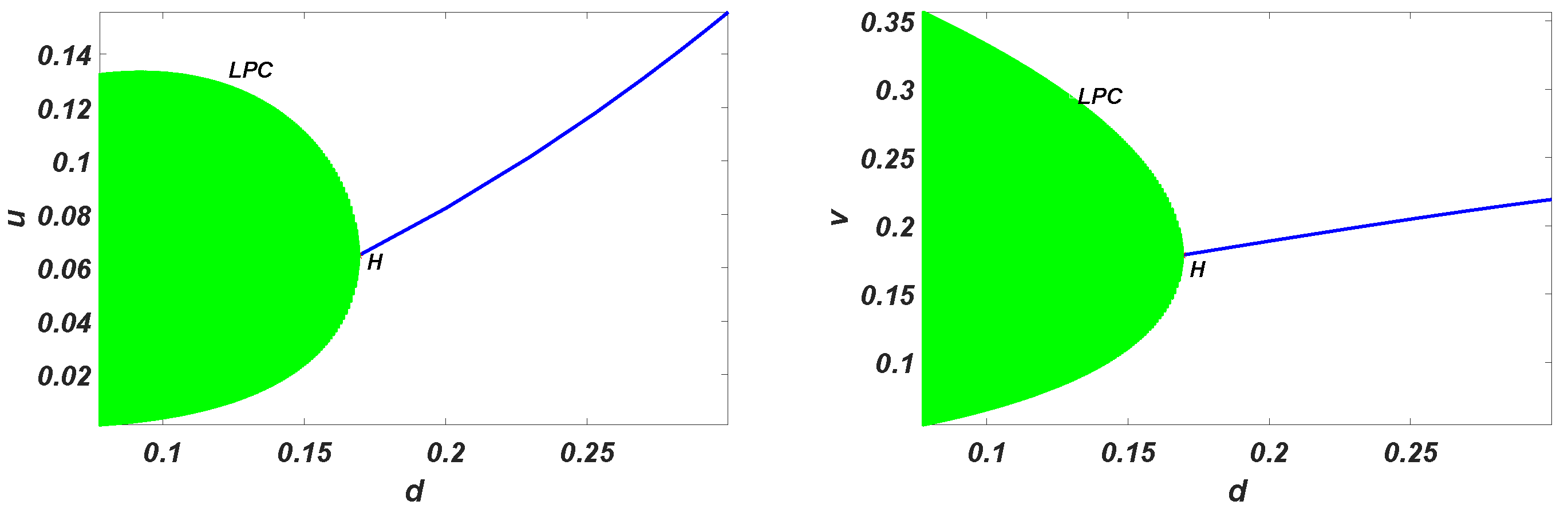
Hopf Bifurcation Analysis

Now, we examine the possibility of Hopf bifurcation with respect to the death rate of predators (d) around E * . Hopf bifurcation is the simple scenario for the models’ stability changes, and periodic solutions emerge. For that, the characteristic roots of Equation (7) should be purely complex. The roots of Equation (7) are
σ 1 , 2 = T r ( J E * ) ± T r ( J E * ) 2 4 D e t ( J E * ) 2
where T r ( J E * ) = α 1 and D e t ( J E * ) = α 2 are the functions of d.
Let the imaginary complex characteristic root of the characteristic Equation (7) be σ 1 , 2 ( d ¯ ) = β 1 ( d ¯ ) ± ι β 2 ( d ¯ ) , which is obtained from α 1 = 0 and α 2 > 0 . From α 1 = 0 , the critical value of d ¯ is
d ¯ = v * γ s v * + u * ( γ 1 ) δ + 4 u * 2 + u * 2 δ 2 u * + 1 + 1 2 u * v * 2 γ δ u * + v * γ 2 .
Theorem 2.
At E * , the model (2) will undergo Hopf bifurcation if the following conditions hold:
1. 
β 1 ( d ¯ ) = 0 ,
2. 
R e ( σ ( d ) ) d = d ¯ 0 .
Proof. 
On substituting σ 1 into Equation (7) and collecting the imaginary and real part, we have
β 1 2 β 2 2 + α 1 β 1 + α 2 = 0 ,
2 β 1 β 2 + α 1 β 2 = 0 .
For d = d ¯ , β 1 ( d ¯ ) = 0 , then Equation (9) reduces to
α 1 β 2 = 0 , and β 2 2 + α 2 = 0 with β 2 0 .
Then, we have α 1 ( d ¯ ) = 0 and β 2 ( d ¯ ) = α 2 ( d ¯ ) , which gives σ ( d ¯ ) = ι α 2 ( d ¯ ) . On substituting β 1 ( d ¯ ) = 0 after differentiating Equation (9) with respect to d, we have
α 1 β 1 ( d ) 2 β 2 β 2 ( d ) = 2 β 2 β 1 ( d ) + α 1 β 2 ( d ) = β 2 α 1 ( d ) .
Solving Equation (12) gives
R e ( σ ( d ) ) d = d ¯ = α 1 α 2 ( d ) + 2 β 2 2 α 1 ( d ) α 1 + 4 β 2 2 d = d ¯ 0 ,
provided α 1 α 2 ( d ) + 2 β 2 2 α 1 ( d ) 0 . □

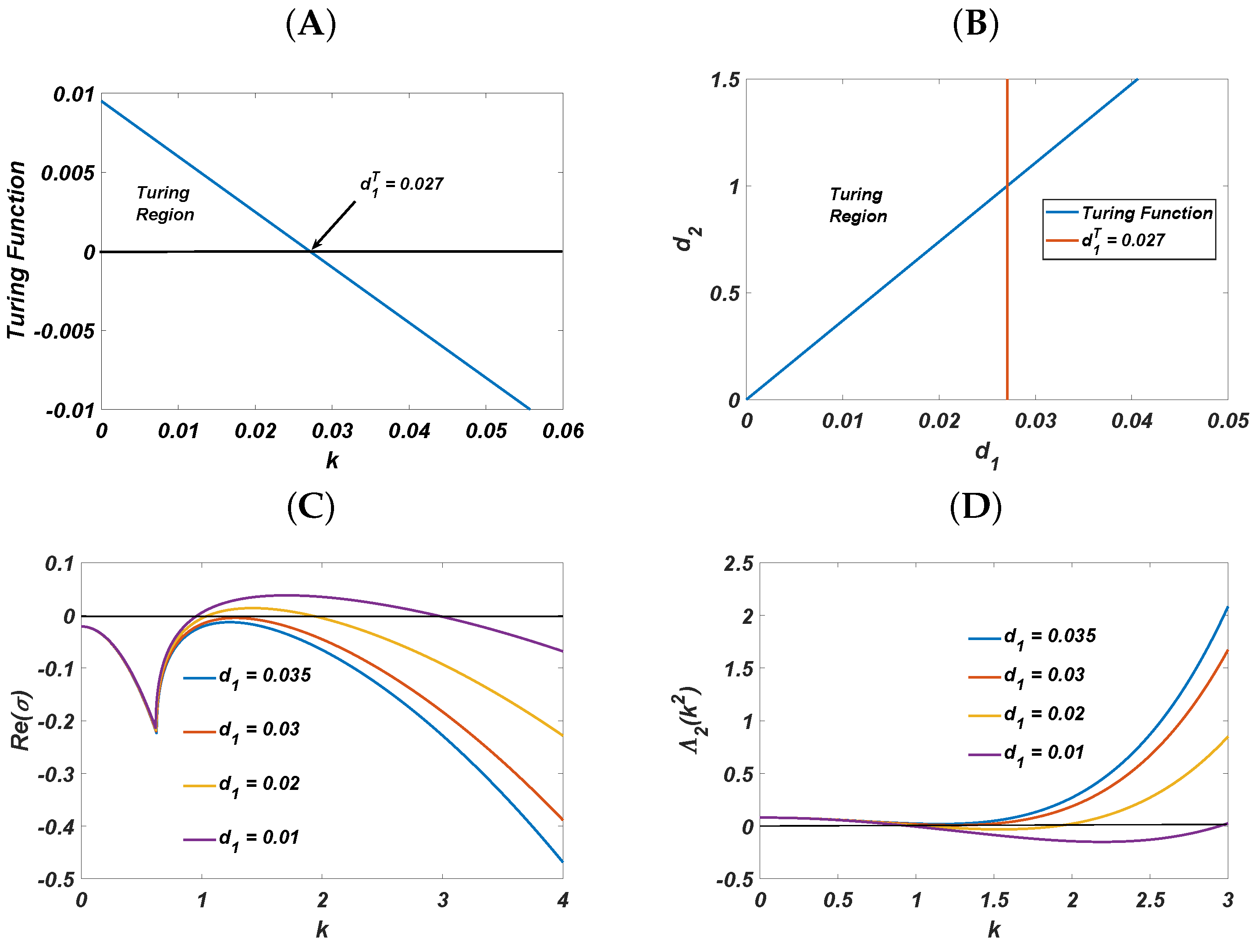
4. Diffusion-Driven Instability

For diffusion-driven instability, we assume that model (2) is temporally stable and linearize model (3) for E * = ( u * , v * ) , which gives
z ˙ = J E * z + D 2 z ,
where
z = u u * v v * , D = d 1 0 0 d 2 ,
and J E * is defined in Equation (6). Let the solution of Equation (14) be
z = ϵ c k e ( σ t + i k . r ) + c . c . + O ( ϵ 2 ) ,
where k is the wave number, r is the spatial vector, i is the imaginary unit ( i 2 = 1 ), σ is the growth rate of perturbation in time t, and c . c . represents the conjugate of the amplitudes associated with the modes k .
Substituting Equation (16) into Equation (14), then
a 11 k 2 d 1 σ a 12 a 21 a 22 k 2 d 2 σ = 0 .
Solving Equation (17) yields the characteristic equation
σ 2 Λ 1 ( k 2 ) σ + Λ 2 ( k 2 ) = 0
where
Λ 1 ( k 2 ) = T r ( J E * ) ( d 1 + d 2 ) k 2 , Λ 2 ( k 2 ) = D e t ( J E * ) ( a 11 d 2 + a 22 d 1 ) k 2 + d 1 d 2 k 4 .
As per A. M. Turing’s theory, the conditions for diffusion-driven instability occur if the system Equation (3) breaks its stability and becomes spatially unstable. Obviously, Λ 1 ( k 2 ) = T r ( J E * ) ( d 1 + d 2 ) k 2 < 0 as T r ( J E * ) < 0 and k , d 1 , d 2 > 0 .
Thus, the only condition that can describe the instability is
Λ 2 ( k 2 ) = D e t ( J E * ) ( a 11 d 2 + a 22 d 1 ) k 2 + d 1 d 2 k 4 < 0 .
for some nonzero k. On differentiating Λ 2 ( k 2 ) with respect to k 2 , we have
Λ 2 ( k m i n 2 ) = D e t ( J E * ) ( a 11 d 2 + a 22 d 1 ) 2 4 d 1 d 2 , k 2 = k m i n 2 = a 11 d 2 + a 22 d 1 2 d 1 d 2 .
Thus, the condition that Λ 2 ( k 2 ) < 0 for some k 2 0 is
D e t ( J E * ) < ( a 11 d 2 + a 22 d 1 ) 2 4 d 1 d 2 .
The critical conditions for Turing bifurcation (Turing instability) are R e ( σ ( k ) ) = 0 and I m ( σ ( k ) ) = 0 , which require the transversal condition to be met and Λ 2 ( k m i n 2 ) = 0 (Turing function), i.e., D e t ( J E * ) = ( a 11 d 2 + a 22 d 1 ) 2 4 d 1 d 2 [15,16].
The critical wave number k = k T is then given (using Equation (20)) by
k T 2 = a 11 d 2 + a 22 d 1 2 d 1 d 2 = D e t ( J E * ) d 1 d 2 .
On substituting the value of k T 2 in Λ 2 ( k 2 ) < 0 , we obtain the critical condition for Turing instability:
( a 11 d 2 + a 22 d 1 ) 2 > 4 ( a 11 a 22 a 21 a 12 ) d 1 d 2 .
The above analysis gives:
Theorem 3.
At E * , the model (3) exhibits diffusion-driven instability if
1. 
a 11 + a 22 < 0 and a 11 a 22 a 12 a 21 > 0 ,
2. 
a 11 d 2 + a 22 d 1 > 0 ,
3. 
( a 11 d 2 + a 22 d 1 ) 2 > 4 ( a 11 a 22 a 21 a 12 ) d 1 d 2
Next, by considering d 1 as a Turing bifurcation parameter, we derive the amplitude equations, and the threshold value of the Turing bifurcation parameter d 1 = d 1 T is presented in Figure 1, along with the region for Turing patterns in the d 1 d 2 plane.

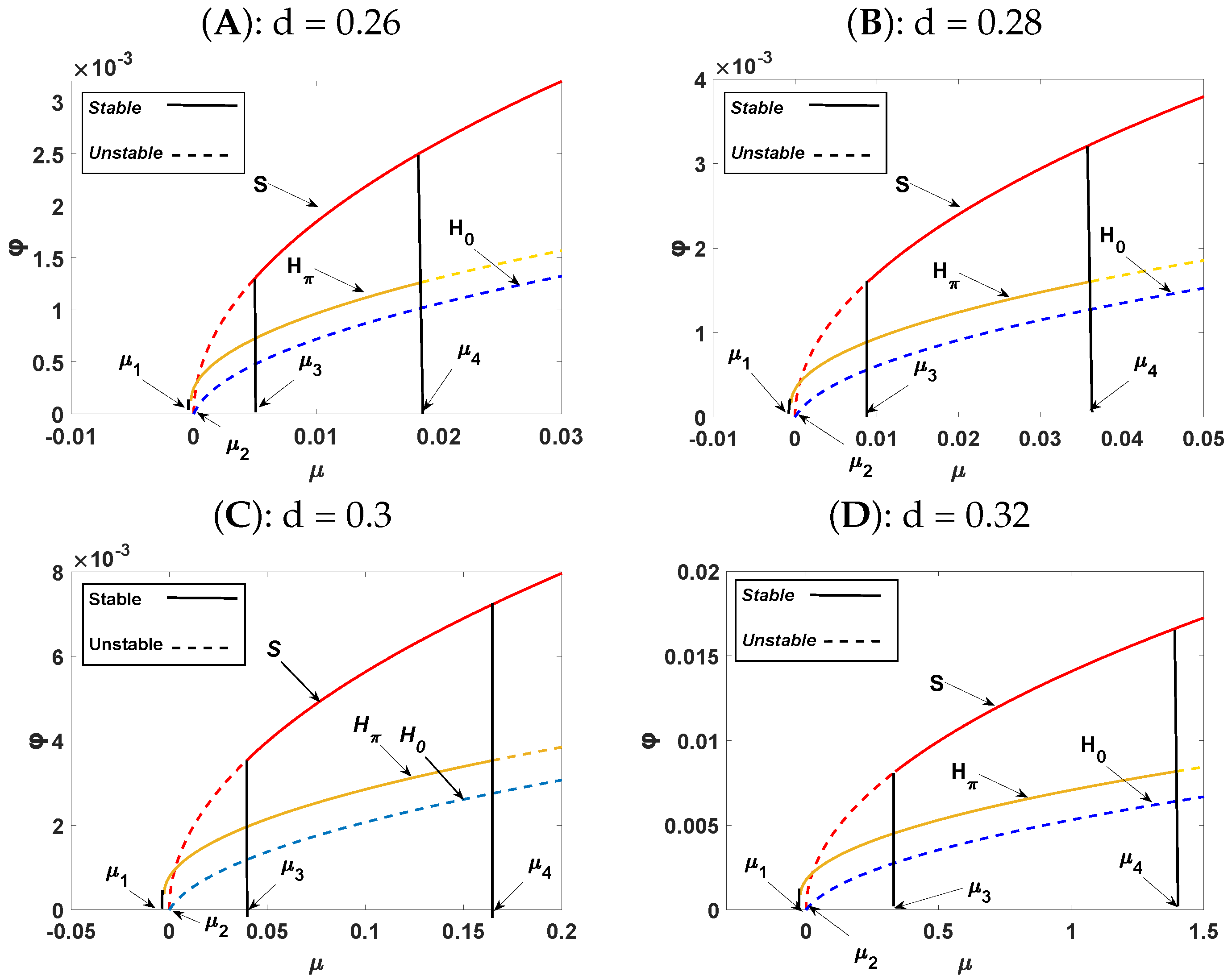
5. Weakly Nonlinear Analysis

In this section, we derive the amplitude equations and analyze the Turing patterns (e.g., spots and stripe patterns) through multiple-scale analysis. These patterns are well described by a system of three active resonant pairs of modes ( k j , k j ) (j = 1,2,3) with an angle of 2 π / 3 , and where | k j | = k T .
First, we linearize the model (3) at E * = ( u * , v * ) , and represent the system in matrix form as:
t u v = a 11 a 12 a 21 a 22 u v + 1 2 f u u u 2 + 2 f u v u v + f v v v 2 g u u u 2 + 2 g u v u v + g v v v 2 + 1 6 f u u u u 3 + 3 f u u v u 2 v + 3 f u v v u v 2 + f v v v v 3 g u u u u 3 + 3 g u u v u 2 v + 3 g u v v u v 2 + g v v v v 3 + d 1 2 u d 2 2 v .
The solution of model (3) near d 1 = d 1 T can be expressed as follows:
U = u v = j = 1 3 C j u C j v e ( i k j . r ) + c . c .
So, Equation (22) can be rewritten as:
U t = U L + N
where L and N represent the linear and nonlinear terms, respectively.
U = [ u , v ] T , L = a 11 + d 1 2 a 12 a 21 a 22 + d 2 2 ,
and
N = ϵ 2 N 2 + ϵ 3 N 3 + O ( ϵ 4 ) , where N 2 = 1 2 f u u u 1 2 + 2 f u v u 1 v 1 + f v v v 1 2 g u u u 1 2 + 2 g u v u 1 v 1 + g v v v 1 2 N 3 = f u u u 1 u 2 + f u v ( u 1 v 2 + u 2 v 1 ) + f v v v 1 v 2 + 1 6 ( f u u u u 1 3 + 3 f u u v u 1 2 v 1 + 3 f u v v u 1 v 1 2 + f v v v v 1 3 ) g u u u 1 u 2 + g u v ( u 1 v 2 + u 2 v 1 ) + g v v v 1 v 2 + 1 6 ( g u u u u 1 3 + 3 g u u v u 1 2 v 1 + 3 g u v v u 1 v 1 2 + g v v v v 1 3 )
Now, we expand the bifurcation parameter d 1 and U through perturbation techniques, as follows:
d 1 T d 1 = ϵ d 1 ( 1 ) + ϵ 2 d 1 ( 2 ) + O ( ϵ 3 ) ,
U = u v = ϵ u 1 v 1 + ϵ 2 u 2 v 2 + ϵ 3 u 3 v 3 + O ( ϵ 4 ) .
On substituting Equation (25) into L, we obtain
L = L T + ϵ d 1 ( 1 ) M + ϵ 2 d 1 ( 2 ) M + O ( ϵ 3 ) ,
where
L T = a 11 + d 1 T 2 a 12 a 21 a 22 + d 2 2 and M = 2 0 0 0 .
At the initial stage, the amplitude C j varies slowly; therefore, T 0 = 0 . Hence, the expansion of time t is
t = ϵ T 1 + ϵ 2 T 2 + O ( ϵ 3 )
On substituting Equations (26)–(29) into Equation (24), we have the 1 s t order ( O ( ϵ ) ):
L T u 1 v 1 = 0 ,
The solution of system Equation (30) is
u 1 v 1 = Υ 1 1 j = 1 3 [ Z j e ( i k j . r ) ] + c . c . ,
where Υ 1 = a 11 d 2 a 22 d 1 T 2 a 21 d 1 T , | k j | = k T * , and Z j is the first-order amplitude of the corresponding e ( i k j . r ) .
For the 2 n d order ( O ( ϵ 2 ) ):
L T u 2 v 2 =   T 1 u 1 v 1 d 1 ( 1 ) M u 1 v 1 N 2 .
By the use of Fredholm solvability condition [39], the zero eigenvectors of L T * are
1 Υ 2 e ( i k j . r ) + c . c . , j = 1 , 2 , 3 .
By the orthogonality condition, we have
1 Υ 2 e ( i k j . r ) N 2 = 0 . j = 1 , 2 , 3 .
where Υ 2 = 2 a 12 d 1 T a 11 d 2 a 22 d 1 T .
From Equation (34), we have
( Υ 1 + Υ 2 ) Z 1 T 1 = k T 2 d 1 ( 1 ) Υ 1 Z 1 + ( f u u Υ 1 2 + f u v Υ 1 + f v v + Υ 2 ( g u u Υ 1 2 + g u v Υ 1 + g v v ) ) Z ¯ 2 Z ¯ 3 , ( Υ 1 + Υ 2 ) Z 2 T 1 = k T 2 d 1 ( 1 ) Υ 1 Z 2 + ( f u u Υ 1 2 + f u v Υ 1 + f v v + Υ 2 ( g u u Υ 1 2 + g u v Υ 1 + g v v ) ) Z ¯ 1 Z ¯ 3 , ( Υ 1 + Υ 2 ) Z 3 T 1 = k T 2 d 1 ( 1 ) Υ 1 Z 3 + ( f u u Υ 1 2 + f u v Υ 1 + f v v + Υ 2 ( g u u Υ 1 2 + g u v Υ 1 + g v v ) ) Z ¯ 1 Z ¯ 2 .
Solving Equation (32) yields
u 2 v 2 = U 0 V 0 + j = 1 3 U j V j e ( i k j . r ) + j = 1 3 U j j V j j e ( i 2 k j . r ) + U 12 V 12 e ( i ( k 1 k 2 ) . r ) + U 23 V 23 e ( i ( k 2 k 3 ) . r ) + U 31 V 31 e ( i ( k 3 k 1 ) . r ) + c . c
where
U 0 V 0 = u 0 v 0 ( | Z 1 | 2 + | Z 2 | 2 + | Z 3 | 2 ) , U j = x V j , U j j V j j = u 11 v 11 Z j 2 , U j k V j k = u * v * Z j Z ¯ k
with
u 0 v 0 = 2 a 12 Q 2 a 22 P a 12 a 21 a 11 a 22 2 a 11 Q a 21 P a 11 a 22 a 12 a 21 , u 11 v 11 = a 22 P + a 12 Q + 4 d 2 P k T 2 4 d 2 k T 2 a 22 a 11 4 d 1 T k T 2 + a 12 a 21 a 21 P a 11 Q + 4 Q d 1 T k T 2 4 d 2 k T 2 a 22 a 11 4 d 1 T k T 2 + a 12 a 21 , u * v * = 2 a 22 P + 2 a 12 Q + 6 d 2 P k T 2 3 d 2 k T 2 a 22 a 11 3 d 1 T k T 2 + a 12 a 21 2 a 21 P 2 a 11 Q + 6 Q d 1 T k T 2 3 d 2 k T 2 a 22 a 11 3 d 1 T k T 2 + a 12 a 21
and
P = ( 1 2 f u u Υ 1 2 + f u v Υ 1 + 1 2 f v v ) , Q = ( 1 2 g u u Υ 1 2 + g u v Υ 1 + 1 2 g v v )
For the 3 r d order ( O ( ϵ 3 ) ):
L T u 3 v 3 = T 1 u 2 v 2 + T 2 u 1 v 1 d 1 ( 1 ) M u 2 v 2 d 1 ( 2 ) M u 1 v 1 N 3
Using the Fredholm solubility condition gives
( Υ 1 + Υ 2 ) Y 1 T 1 + Z 1 T 2 = k T 2 Υ 1 ( d 1 2 Z 1 + d 1 1 Y 1 ) + [ f u u Υ 1 2 + 2 f u v Υ 1 + f v v + Υ 2 ( g u u Υ 1 2 + 2 g u v Υ 1 + g v v ) ] ( Z ¯ 2 Y ¯ 3 + Z ¯ 3 Y ¯ 2 ) ( G 1 | Z 1 | 2 + G 2 ( | Z 2 | 2 + | Z 3 | 2 ) Z 1 )
where G 1 = ( I 1 + Υ 2 J 1 ) , G 2 = ( I 2 + Υ 2 J 2 ) , and
I 1 = [ ( Υ 1 f u u + f u v ) ( u 0 + u 11 ) + ( f v v + Υ 1 f u v ) ( v 0 + v 11 ) + R ] , I 2 = [ ( Υ 1 f u u + f u v ) ( u 0 + u * ) + ( f v v + Υ 1 f u v ) ( v 0 + v * ) + A ] , J 1 = [ ( Υ 1 g u u + g u v ) ( u 0 + u 11 ) + ( g v v + Υ 1 g u v ) ( v 0 + v 11 ) + S ] , J 2 = [ ( Υ 1 g u u + g u v ) ( u 0 + u * ) + ( g v v + Υ 1 g u v ) ( v 0 + v * ) + B ] , R = 1 2 f u u u Υ 1 3 + 3 2 f u u v Υ 1 2 + 3 2 f u v v Υ 1 + 1 2 f v v v , S = 1 2 g u u u Υ 1 3 + 3 2 g u u v Υ 1 2 + 3 2 g u v v Υ 1 + 1 2 g v v v , A = f u u u Υ 1 3 + 3 f u u v Υ 1 2 + 3 f u v v Υ 1 + f v v v , B = g u u u Υ 1 3 + 3 g u u v Υ 1 2 + 3 g u v v Υ 1 + g v v v .
On changing the subscript of Z, we obtain the other two equations.
The Taylor series expansion of amplitude C j (j = 1, 2, 3) can be expressed as follows:
C j = ϵ Z j + ϵ 2 Y j + O ( ϵ 3 )
From Equations (40) and (41), we have
τ 0 C 1 t = μ C 1 + h C ¯ 2 C ¯ 3 [ b 1 | C 1 | 2 + b 2 ( | C 2 | 2 + | C 3 | 2 ) ] C 1 , τ 0 C 2 t = μ C 2 + h C ¯ 1 C ¯ 3 [ b 1 | C 2 | 2 + b 2 ( | C 3 | 2 + | C 1 | 2 ) ] C 2 , τ 0 C 3 t = μ C 3 + h C ¯ 1 C ¯ 2 [ b 1 | C 3 | 2 + b 2 ( | C 1 | 2 + | C 2 | 2 ) ] C 3 .
where
τ 0 = ( Υ 1 + Υ 2 ) Υ 1 d 1 T k T 2 , μ = d 1 T d 1 d 1 T , h = 2 ( P + Υ 2 Q ) Υ 1 d 1 T k T 2 , b 1 = G 1 Υ 1 d 1 T k T 2 , b 2 = G 2 Υ 1 d 1 T k T 2 .
Equation (42) is called the amplitude equation up to the third order of perturbation. Next, we investigate amplitude stability analysis; on substituting C j = φ j exp ( i ϕ j ) into Equation (42) and collecting the real and imaginary part, we obtain
τ 0 ϕ t = h φ 1 2 φ 2 2 + φ 2 2 φ 3 2 + φ 3 2 φ 1 2 φ 1 φ 2 φ 3 sin ϕ , τ 0 φ 1 t = μ φ 1 + h φ 2 φ 3 cos ϕ b 1 φ 1 3 b 2 ( φ 2 2 + φ 3 2 ) φ 1 , τ 0 φ 2 t = μ φ 2 + h φ 3 φ 1 cos ϕ b 1 φ 2 3 b 2 ( φ 3 2 + φ 1 2 ) φ 2 , τ 0 φ 3 t = μ φ 3 + h φ 1 φ 2 cos ϕ b 1 φ 3 3 b 2 ( φ 1 2 + φ 2 2 ) φ 2 ,
where ϕ = ϕ 1 + ϕ 2 + ϕ 3 .
The solutions of system Equation (44) are as follows:
  • The first solution: The stationary state is represented by φ 1 = φ 2 = φ 3 = 0 , which is stable for μ < μ 2 = 0 and unstable for μ > μ 2 = 0 .
  • The second solution: The stripe pattern given by φ 1 = μ b 1 0 , φ 2 = φ 3 = 0 is stable for μ > μ 3 = h 2 b 1 ( b 2 b 1 ) 2 and unstable for μ < μ 3 .
  • The third solution: When μ > μ 1 , two solutions exist: Hexagon patterns are given by φ 1 = φ 2 = φ 3 = | h | ± h 2 + 4 ( b 1 + 2 b 2 ) μ 2 ( b 1 + 2 b 2 ) with ϕ = 0 or π , and exist when μ > μ 1 = h 2 4 ( b 1 + 2 b 2 ) ; the solution φ + = | h | + h 2 + 4 ( b 1 + 2 b 2 ) μ 2 ( b 1 + 2 b 2 ) is stable for μ < μ 4 = 2 b 1 + b 2 ( b 2 b 1 ) 2 h 2 , and φ = | h | h 2 + 4 ( b 1 + 2 b 2 ) μ 2 ( b 1 + 2 b 2 ) is unstable.
  • The mixed states: When φ 1 = | h | b 2 b 1 , φ 2 = φ 3 = μ b 1 φ 1 2 b 1 + b 2 , with b 2 > b 1 . This exists when μ > μ 3 and is always unstable.
From all the above analyses, we bind up all the results in the form of a theorem.
Theorem 4.
The model Equation (3) possesses four different kinds of patterns, and their stability is described as:
1. 
Homogeneous solution:  It is stable for μ < μ 2 and unstable for μ > μ 2 .
2. 
Stripe solution:  It is stable for μ > μ 3 and unstable for μ < μ 3 .
3. 
Hexagonal solution:  It exists when μ > μ 1 and φ + is stable for μ < μ 4 and φ is always unstable.
4. 
Mixed solution:  It exists but is always unstable when b 2 > b 1 and μ > μ 3 .

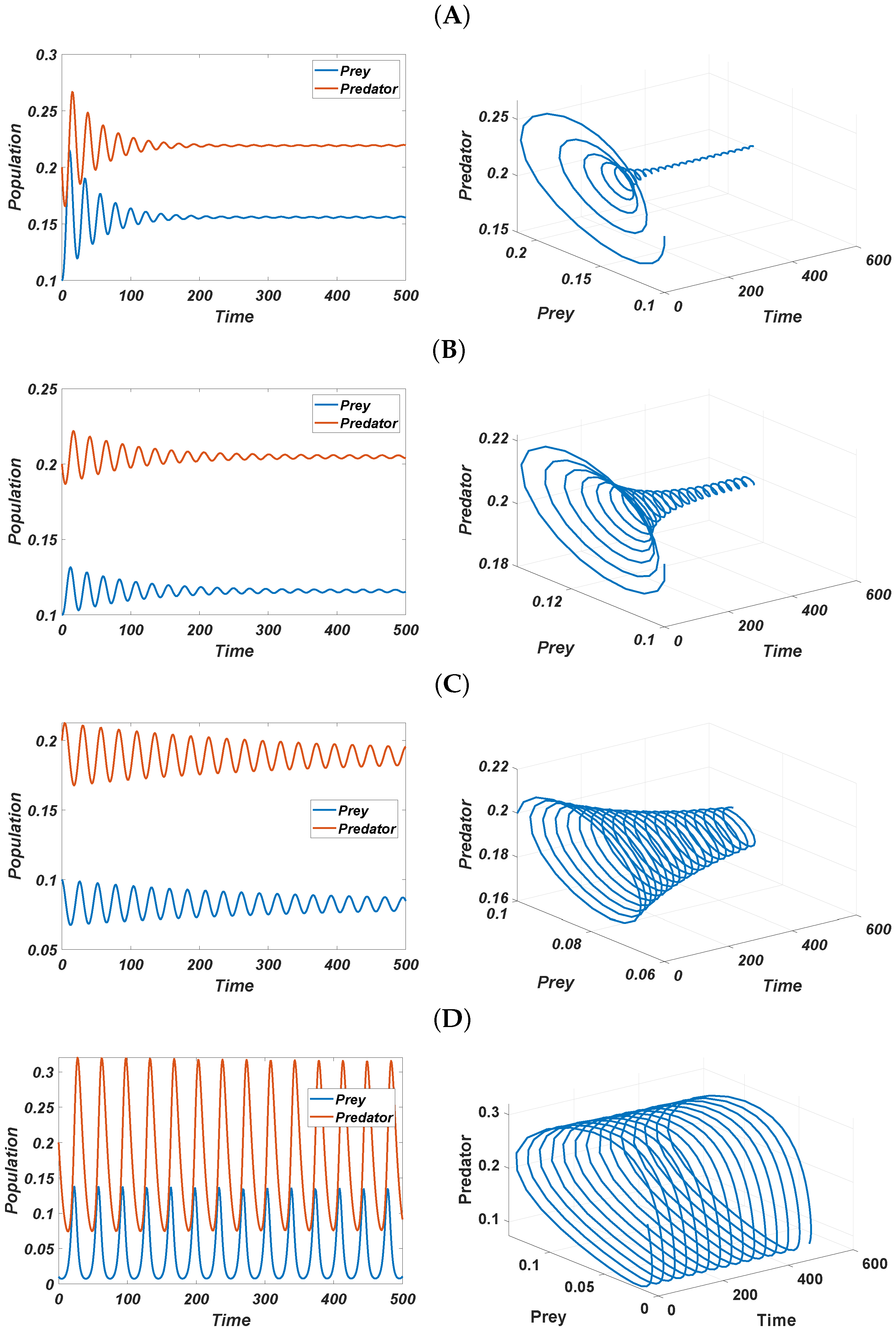
6. Numerical Simulations

In this section, we analyze the results of numerical simulations to verify the theoretical results from the preceding sections. The simulation facilitates understanding the nonspatial and spatial dynamics of model (2) and (3), respectively. For numerical simulations, we fixed the parameter’s numerical value: s = 2 , γ = 2 3 , δ = 1 , and d 2 = 1 ; and consider d and d 1 as the controlled parameters [14].
Using the value of fixed parameters and d = 0.3 , the model (2) has three equilibrium points: ( 0 , 0 ) , ( 1 , 0 ) , and ( 0.1558 , 0.2192 ) . Since the analysis is focused on coexistence equilibrium point E * = ( 0.1558 , 0.2192 ) , we therefore check the stability first: T r ( J E * ) = 0.0697734 < 0 and D e t ( J E * ) = 0.0644773 > 0 . From Routh–Hurwitz stability criteria and Theorem 1, the model (2) is asymptotically stable at E * .

6.1. Nonspatial Analysis

Now, we study the nonspatial analysis of the model (2) to check the influence of the natural death rate of predators on the prey–predator system. In Figure 2, we describe the time evolution of the population and corresponding phase portrait for different values of the parameter d = 0.3 , 0.25 , 0.2 , 0.12 . As the value of d decreases, the model loses its stability; for d = 0.3 , we observe a stable focus on the equilibrium point, whereas for d = 0.12 , we obtain a limit cycle for the equilibrium point, Meanwhile, in Figure 3, we perform Hopf bifurcation analysis over the bifurcation parameter d ( 0.05 , 0.3 ) : for the small value of d < d ¯ = 0.17 , the model shows unstable steady states, and for the large value of d > d ¯ = 0.17 , the model is stable. From the nonspatial analysis, it is very clear that the death rate of predators plays a vital role in the stability of the prey–predator system.

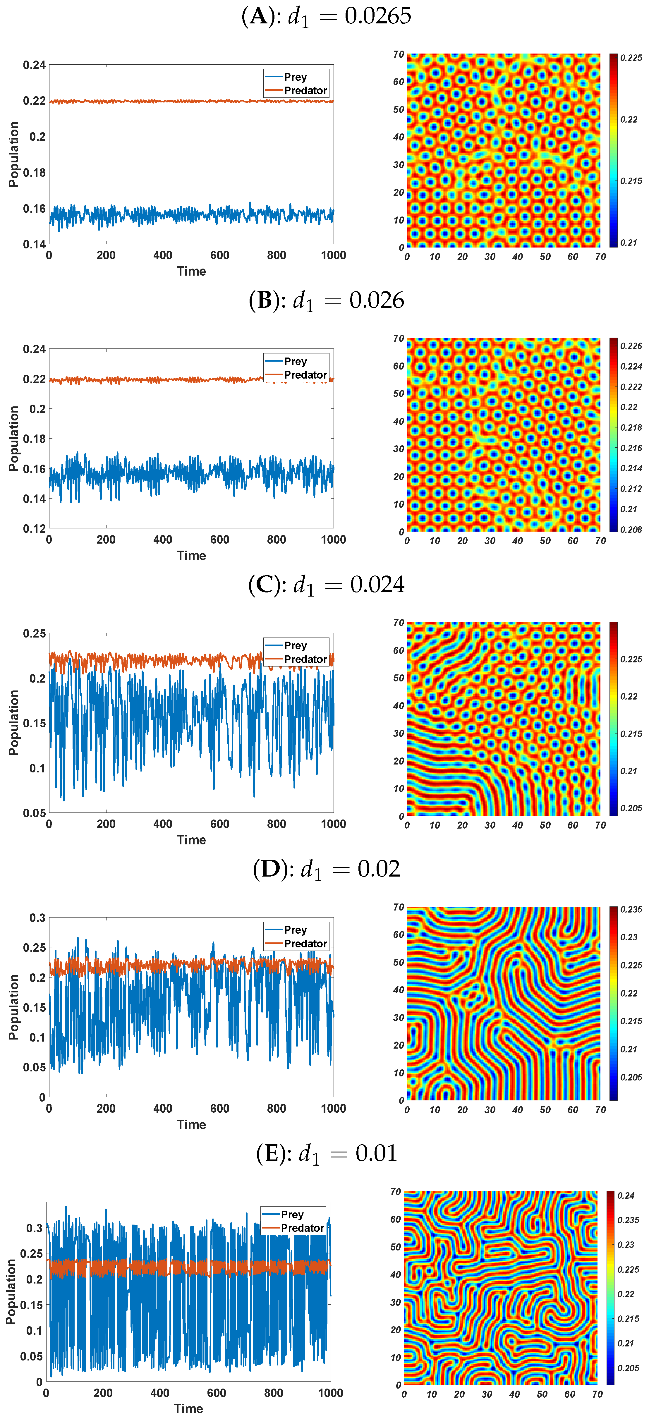
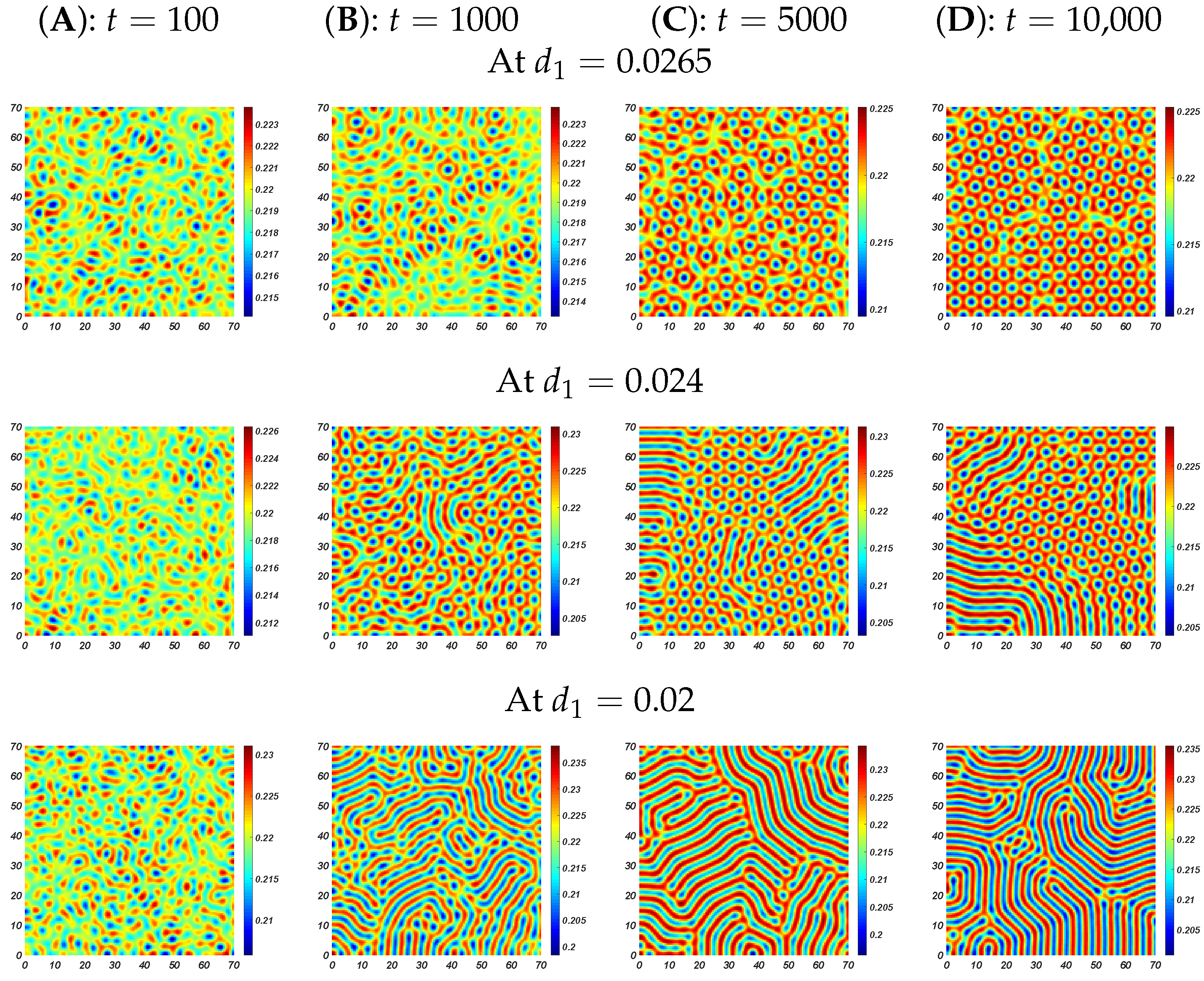
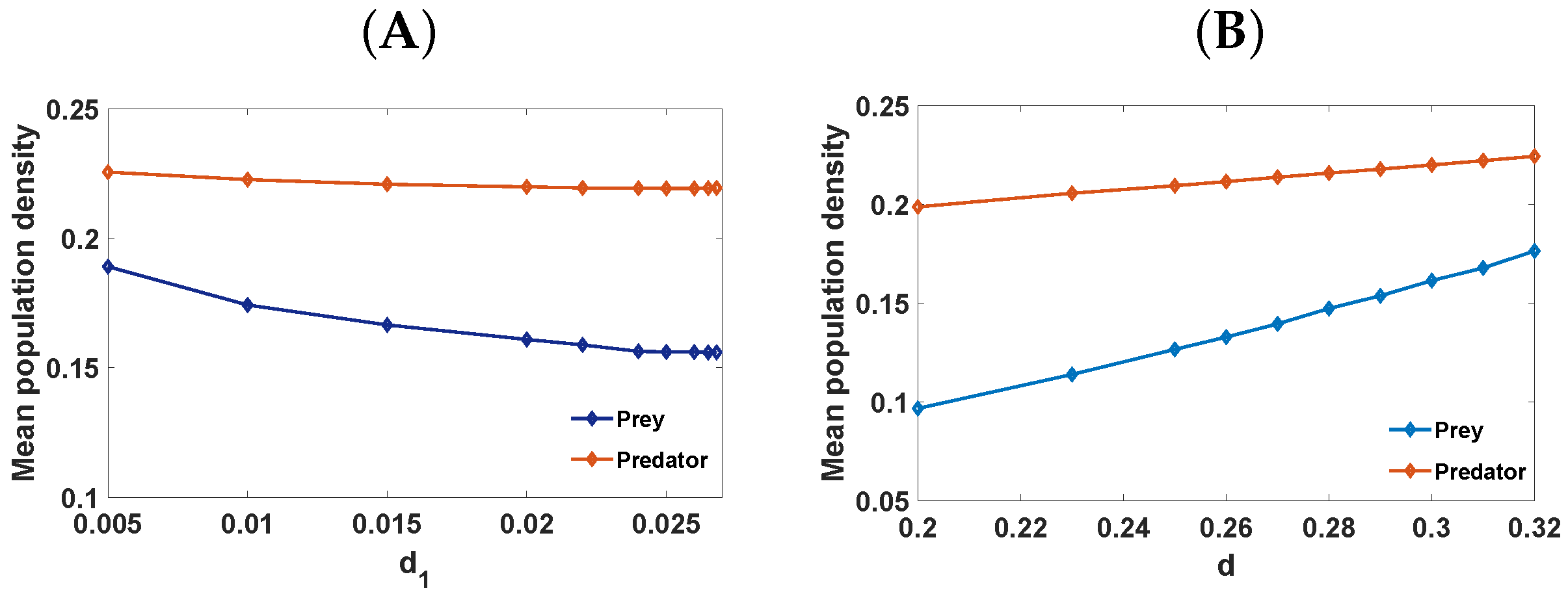
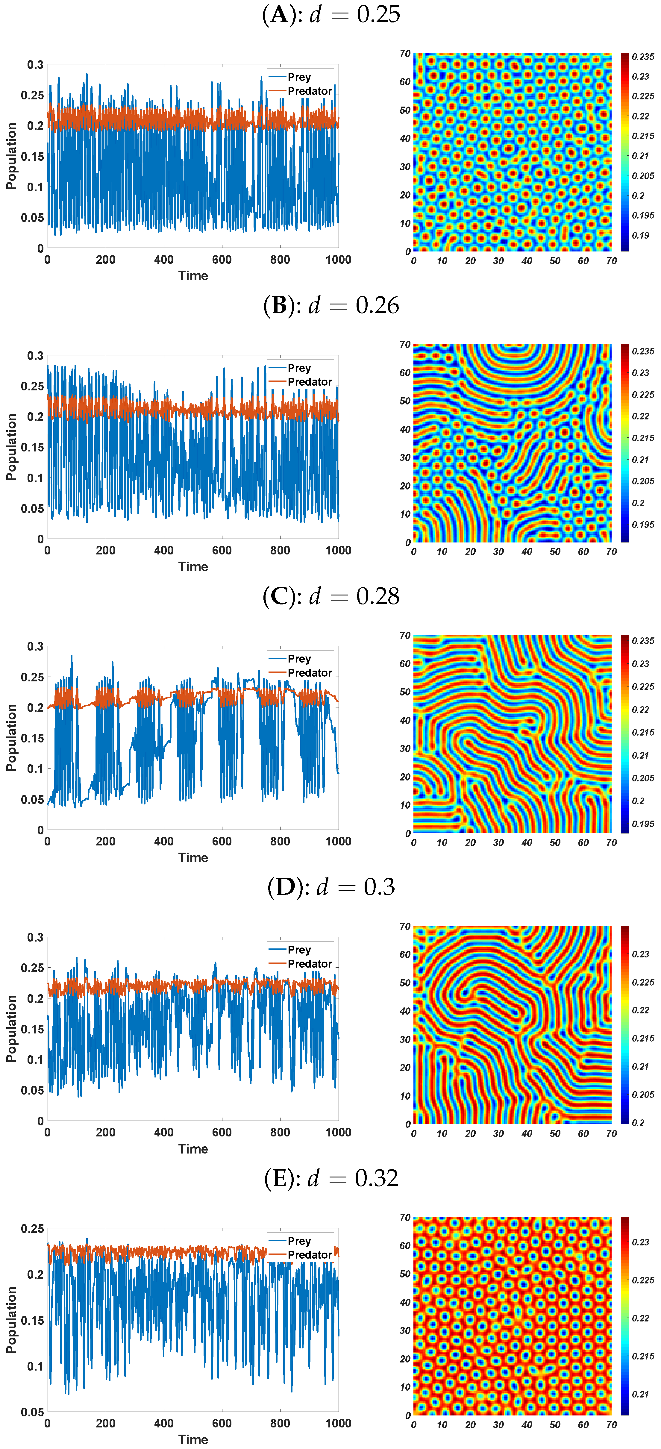
6.2. Pattern Selection

We performed pattern selection for model (3) in a 2D space of size [ 0 , 70 ] × [ 0 , 70 ] . To solve the diffusive model (3), we used FDM (finite difference method), and EM (Euler method) approximation with Δ t = 0.1 (time step), Δ x = 0.5 = Δ y (space step), and the initial condition as
u ( x i , y j , 0 ) = u * + 0.01 ϱ i j * , v ( x i , y j , 0 ) = v * + 0.01 ϱ i j *
where ϱ i j * are statistically uncorrelated Gaussian white noise perturbations with zero mean and fixed variance in two-dimensional space. The simulations are intended to reveal patterns by changing the controlled parameters d 1 and d with fixed parameters value under zero-flux boundary conditions.
In Figure 1, we graphically show the Turing bifurcation threshold value and region where different patterns are obtained. From Figure 1, it is very clear that when d 1 < d 1 T , diffusion-driven instability occurs. However, the type of pattern structure is unknown. So, we employed the amplitude equation to analyze the formation of Turing patterns close to onset d 1 = d 1 T .
From amplitude stability analysis over the different values of parameter d and fixed d 1 = 0.02 and d 2 = 1 , we have the corresponding values of d 1 T , b 1 , b 2 , μ 1 , μ 2 , μ 3 , and μ 4 , as seen in Table 2. The bifurcation diagram of amplitude φ versus μ is presented in Figure 4, where the solid curves denote stable states and dotted curves represent unstable states; S, H π , and H 0 represent the stripe pattern, hexagonal pattern with ϕ = π , and hexagonal pattern with ϕ = 0 , respectively. The stability and the existence range of the four solutions are displayed in Theorem 4. From the numerical simulations, we have the same patterns of predators as those of prey. So, we display the spatial distribution of the predator population, where the colors red (high) and blue (low) represent the population density.
Effects of varying d 1 on pattern formation
For varying values of d 1 and a fixed d = 0.3 , the system (3) has the following Turing patterns: spots, mixed, and stripes. From Figure 1A: the value of d 1 ( 0 , d 1 T ) , at which Turing patterns appear. In Table 3, the μ values corresponding to different d 1 are presented, and from the amplitude stability, we identify the regions exhibiting various Turing patterns. In Figure 5, we show the time-series solution of the model (3) in the first panel at T = 1000 , where we observe the dynamical behavior of the system in space for different values of d 1 . When d 1 ( 0 , d 1 T ) , the corresponding Turing patterns are presented in Figure 5’s second panel: as the controlled parameter d 1 decreases, the patterns of spots→ mixed → stripes is obtained at t = 10 , 000 . The stability of these Turing patterns is discussed in Figure 6. From Figure 5 and Table 3, we conclude that the numerical results correspond to the theoretical analyses.
Ecologically, the diffusion coefficient d 1 significantly affects Turing selection and shows various spatial patterns. In Figure 7A, we show the mean population density of species for varying diffusion rates of prey. It is very clear from the graphical result that more dispersal among prey species will reduce the prey population. Biologically, this may be due to the fact that more broad distribution among prey species will increase the hunt rate by predators, because predators will obtain more prey quickly for their nourishment, reducing the prey population.
Effects of varying d on pattern formation
Now, we study the influence of the death rate of predators (d) on a spatial scale via Turing patterns. The larger the value of d, the smaller the size of the group will be. Thus, the predator death rate significantly affects the spatial distribution of the population. In Figure 8, the first panel shows the time-series solution of the model (3) at T = 1000 , whereas the second panel has the patterns for model (3) corresponding to d = 0.25 , 0.26 , 0.28 , 0.3 , 0.32 . From the amplitude stability analysis that is discussed in Table 2 and Figure 4, we have spot patterns; Figure 8A,B present spot and mixed patterns for d = 0.25 and d = 0.26 , respectively. For d = 0.28 , 0.3 , stripe patterns are observable (Figure 8C,D). When d = 0.32 , a black eye pattern is detectable at time t = 5000 (see Figure 8E). These patterns show the spatial structure formed by the species in the domain; thus, they have a clear ecological meaning. For γ = 2 3 , the predator population forms a small fixed number of groups. As d increases (0.25→0.32), the red spots get converted into blue spots, which indicates that the as the value of d increases, the population of species stabilizes. In Figure 7B, we show the spatial mean population density of species with varying death rates among predators.
The results of Figure 7B and Figure 8 show that when predators’ death rates increase, the prey population increases due to low capture rates by predators. However, a drastic change is noticed in the predator population, and their population also increases. Biologically, this could be because predators form small groups, and when the death rate rises, the young predators receive adequate sustenance, increasing the predator population.

7. Conclusions

The present article discusses the temporal and spatiotemporal dynamics and pattern formation of prey–predator interaction with H-V functional response to examine the influence of spatial dispersal on the population. The H-V constant in functional response defines the size of population-formed groups. Many species in the ecosystem do not form a fixed number of groups. Hence, we focused on prey–predator interaction where predators do not form a fixed number of groups. First, we defined the diffusive mathematical model, and analyzed the model’s temporal stability through the Lyapunov stability theory and the impact of the controlled parameter d through Hopf bifurcation analysis. With the incorporation of diffusion, we derived the condition for “diffusion-driven instability”, which is responsible for the origination of Turing patterns. The amplitude equation for the active modes close to d 1 = d 1 T was derived using multiple-scale analysis. Finally, the theoretical results were validated using numerical simulations. We observed various patterns emerging from the system, such as spot, mixed, and stripe patterns for varying the controlled parameters d 1 and d. Therefore, the numerical results cater to the previous theoretical finding.
Thus, we conclude that variation in self-diffusion d 1 and in predator death rate d change the spatial distribution of the population, resulting in diverse spatial patterns. These results suggest that the mortality rate and diffusion coefficient can affect the system’s dynamics. From a biological perspective, our analysis concludes that in the prey–predator model with predators not forming a fixed number of groups, the death rate among predators plays a vital role in stabilizing the system. Moreover, dispersal among prey species decreases the prey population, because more dispersal among prey species will increase the capturing rate by predators.
In this article, we have shown the influence of control parameters on the prey–predator model on a spatial scale. This method can be applied in research on pattern formation in prey–predator models and in explaining certain field observations. Further investigations into the effects of other biological parameters on spatial distribution and the influence of time delay in biological processes in this model are warranted.

Author Contributions

Conceptualization, S.; methodology, S. and T.S.; software, T.S., N.V. and K.U.S.; validation, T.S., N.V. and K.U.S.; formal analysis, S. and M.K.; investigation, S., T.S. and M.K.; resources, T.S., M.K. and V.V.; data curation, T.S.; writing—original draft preparation, T.A., T.S., N.V., K.U.S. and V.V.; writing—review and editing, T.S. and N.V.; visualization, T.S., N.V. and K.U.S.; supervision, T.S.; project administration, T.S.; funding acquisition, T.A. All authors have read and agreed to the published version of the manuscript.

Funding

This research received no external funding.

Institutional Review Board Statement

Not applicable.

Informed Consent Statement

Not applicable.

Data Availability Statement

Not applicable.

Acknowledgments

Teekam Singh, Vrince Vimal, and Kamred Udham Singh wish to express their heartfelt thanks to the Graphic Era Educational Society for supporting this research.

Conflicts of Interest

The authors declare no conflict of interest.

References

  1. Cresswell, W.; Quinn, J.L. Faced with a choice, sparrowhawks more often attack the more vulnerable prey group. Oikos 2004, 104, 71–76. [Google Scholar] [CrossRef]
  2. Krause, J.; Godin, J.G.J. Predator preferences for attacking particular prey group sizes: Consequences for predator hunting success and prey predation risk. Anim. Behav. 1995, 50, 465–473. [Google Scholar] [CrossRef]
  3. Fitzgibbon, C.D. Mixed-species grouping in Thomson’s and Grant’s gazelles: The antipredator benefits. Anim. Behav. 1990, 39, 1116–1126. [Google Scholar] [CrossRef]
  4. Bailey, I.; Myatt, J.P.; Wilson, A.M. Group hunting within the Carnivora: Physiological, cognitive and environmental influences on strategy and cooperation. Behav. Ecol. Sociobiol. 2013, 67, 1–17. [Google Scholar] [CrossRef]
  5. Scheel, D. Profitability, encounter rates, and prey choice of African lions. Behav. Ecol. 1993, 4, 90–97. [Google Scholar] [CrossRef]
  6. Seo, G.; DeAngelis, D.L. A predator-prey model with a Holling type I functional response including a predator mutual interference. J. Nonlinear Sci. 2011, 21, 811–833. [Google Scholar] [CrossRef]
  7. Singh, T.; Dubey, R.; Mishra, V.N. Spatial dynamics of a predator-prey system with hunting cooperation in predators and type I functional response. AIMS Math. 2020, 5, 673–684. [Google Scholar] [CrossRef]
  8. Singh, T.; Banerjee, S. Spatial aspect of hunting cooperation in predators with Holling type II functional response. J. Biol. Syst. 2018, 26, 511–531. [Google Scholar] [CrossRef]
  9. Fu, S.; Zhang, H. Effect of hunting cooperation on the dynamic behavior for a diffusive Holling type II predator-prey model. Commun. Nonlinear Sci. Numer. Simul. 2021, 99, 105807. [Google Scholar] [CrossRef]
  10. Huang, Y.; Chen, F.; Zhong, L. Stability analysis of a prey-predator model with Holling type III response function incorporating a prey refuge. Appl. Math. Comput. 2006, 182, 672–683. [Google Scholar] [CrossRef]
  11. Agarwal, M.; Pathak, R. Harvesting and Hopf Bifurcation in a prey-predator model with Holling Type IV Functional Response. Int. J. Math. Soft Comput. 2017, 2, 99. [Google Scholar] [CrossRef]
  12. Upadhyay, R.K.; Naji, R.K. Dynamics of a three species food chain model with Crowley-Martin type functional response. Chaos Solit. Fractals 2009, 42, 1337–1346. [Google Scholar] [CrossRef]
  13. Zhang, X.C.; Sun, G.Q.; Jin, Z. Spatial dynamics in a predator-prey model with Beddington-DeAngelis functional response. Phys. Rev. E 2012, 85, 021924. [Google Scholar] [CrossRef] [PubMed]
  14. Hsu, S.B.; Hwang, T.W.; Kuang, Y. Global dynamics of a predator-prey model with Hassell-Varley type functional response. Discret. Contin. Dyn. Syst. Ser. B 2008, 10, 857. [Google Scholar] [CrossRef]
  15. Murray, J. A pre-pattern formation mechanism for animal coat markings. J. Theor. Biol. 1981, 88, 161–199. [Google Scholar] [CrossRef]
  16. Turing, A.M. The chemical basis of morphogenesis. Bull. Math. Biol. 1990, 52, 153–197. [Google Scholar] [CrossRef]
  17. Medvinsky, A.B.; Petrovskii, S.V.; Tikhonova, I.A.; Malchow, H.; Li, B.L. Spatiotemporal complexity of plankton and fish dynamics. SIAM Rev. 2002, 44, 311–370. [Google Scholar] [CrossRef]
  18. Segel, L.A.; Jackson, J.L. Dissipative structure: An explanation and an ecological example. J. Theor. Biol. 1972, 37, 545–559. [Google Scholar] [CrossRef]
  19. Agiza, H.N.; Elabbasy, E.M.; ElMetwally, H.; Elsadany, A.A. Chaotic dynamics of a discrete prey-predator model with Holling type II. Nonlinear Anal. Real World Appl. 2009, 10, 116–129. [Google Scholar] [CrossRef]
  20. Capone, F.; Carfora, M.F.; De Luca, R.; Torcicollo, I. Turing patterns in a reaction diffusion system modeling hunting cooperation. Math. Comput. Simul. 2019, 165, 172–180. [Google Scholar] [CrossRef]
  21. Hao, W.; Xue, C. Spatial pattern formation in reaction-diffusion models: A computational approach. J. Math. Biol. 2020, 80, 521–543. [Google Scholar] [CrossRef] [PubMed]
  22. Pal, S.; Pal, N.; Samanta, S.; Chattopadhyay, J. Effect of hunting cooperation and fear in a predator-prey model. Ecol. Complex. 2019, 39, 100770. [Google Scholar] [CrossRef]
  23. Singh, T.; Dubey, R.; Mishra, V.N.; Abdel-Aty, M. Modeling of Diffusive Patterns in Predator-Prey System using Turing Instability and Amplitude Equations. Inf. Sci. Lett. 2021, 10, 5–16. [Google Scholar]
  24. Song, Q.; Yang, R.; Zhang, C.; Tang, L. Bifurcation analysis of a diffusive predator-prey model with Monod-Haldane functional response. Int. J. Bifurc. Chaos 2019, 29, 1950152. [Google Scholar] [CrossRef]
  25. Wang, J.S.; Wu, Y.P.; Li, L.; Sun, G.Q. Effect of mobility and predator switching on the dynamical behavior of a predator-prey model. Chaos Solit. Fractals 2020, 132, 109584. [Google Scholar] [CrossRef]
  26. Yuan, S.; Xu, C.; Zhang, T. Spatial dynamics in a predator-prey model with herd behavior. Chaos 2013, 23, 033102. [Google Scholar] [CrossRef]
  27. Zhang, T.; Xing, Y.; Zang, H.; Han, M. Spatio-temporal dynamics of a reaction-diffusion system for a predator-prey model with hyperbolic mortality. Nonlinear Dyn. 2014, 78, 265–277. [Google Scholar] [CrossRef]
  28. Kumar, V.; Kumari, N. Stability and bifurcation analysis of Hassell-Varley prey-predator system with fear effect. Int. J. Appl. Comput. Math. 2020, 6, 150. [Google Scholar] [CrossRef]
  29. Li, H.; Tian, Y. Dynamic behavior analysis of a feedback control predator-prey model with exponential fear effect and Hassell-Varley functional response. J. Frankl. Inst. 2023, 360, 3479–3498. [Google Scholar] [CrossRef]
  30. Du, B.; Hu, M.; Lian, X. Dynamical behavior for a stochastic predator-prey model with HV type functional response. Bull. Malays. Math. Sci. Soc. 2017, 40, 487–503. [Google Scholar] [CrossRef]
  31. Xie, X.; Zhang, C.; Chen, X.; Chen, J. Almost periodic sequence solution of a discrete Hassell-Varley predator-prey system with feedback control. Appl. Math. Comput. 2015, 268, 35–51. [Google Scholar] [CrossRef]
  32. Kim, H.K.; Baek, H. The dynamical complexity of a predator-prey system with Hassell-Varley functional response and impulsive effect. Math. Comput. Simul. 2013, 94, 1–14. [Google Scholar] [CrossRef]
  33. Pathak, S.; Maiti, A.; Samanta, G.P. Rich dynamics of a food chain model with Hassell-Varley type functional responses. Appl. Math. Comput. 2009, 208, 303–317. [Google Scholar] [CrossRef]
  34. Zhang, Y.; Gao, S.; Fan, K.; Wang, Q. Asymptotic behavior of a non-autonomous predator-prey model with Hassell-Varley type functional response and random perturbation. J. Appl. Math. Comput. 2015, 49, 573–594. [Google Scholar] [CrossRef]
  35. Luo, D.; Wang, D. Impact of discontinuous harvesting policies on prey-predator system with Hassell-Varley type functional response. Int. J. Biomath. 2017, 10, 1750048. [Google Scholar] [CrossRef]
  36. Chen, D.; Wang, D. Almost periodic dynamics of delayed prey-predator model with discontinuous harvesting policies and Hassell-Varley type functional response. Int. J. Biomath. 2018, 11, 1850083. [Google Scholar] [CrossRef]
  37. Wang, K.; Zhu, Y.L. Permanence and global asymptotic stability of a delayed predator-prey model with Hassell-Varley type functional response. Bull. Iran. Math. Soc. 2011, 37, 197–215. [Google Scholar]
  38. Xu, C.; Li, P. Oscillations for a delayed predator-prey model with Hassell-Varley-type functional response. C. R. Biol. 2015, 338, 227–240. [Google Scholar] [CrossRef]
  39. Skubachevskii, A.L. On necessary conditions for the Fredholm solvability of nonlocal elliptic problems. Proc. Steklov Inst. Math. 2008, 260, 238–253. [Google Scholar] [CrossRef]
Figure 1. (A) The value of the Turing bifurcation parameter corresponding to the diffusion−driven instability. (B) Turing region in the d 1 d 2 plane. (C) Plot of R e ( σ ) versus k for varying d 1 . (D) Plot of Λ 2 ( k 2 ) versus k for varying d 1 . Fixed parameters: s = 2 , γ = 2 3 , δ = 1 , d = 0.3 , and d 2 = 1 .
Symmetry 15 00986 g001
Figure 2. (Left) Time evolution of the population; (Right) phase portrait for system (2). Parameters: s = 2 , γ = 2 3 , and δ = 1 with varying value of d: (A): d = 0.3 , (B): d = 0.25 , (C): d = 0.2 , and (D): d = 0.12 .
Symmetry 15 00986 g002
Figure 3. The bifurcation diagrams with respect to d for model (2), where blue solid curves represent the stable steady state, limit point cycle (LPC), Hopf bifurcation point (H), and the periodic solution (green color region). With s = 2 , γ = 2 3 , δ = 1 .
Symmetry 15 00986 g003
Figure 4. Bifurcation diagram of amplitude φ versus μ with different values of d for model (3). S: strip patterns, H 0 : hexagonal patterns ( ϕ = 0 ), and H π : hexagonal patterns ( ϕ = π ). Fixed parameters: s = 2 , γ = 2 3 , δ = 1 , d 1 = 0.02 , and d 2 = 1 .
Symmetry 15 00986 g004
Figure 5. (Left) Time−series evolution of the populations of the model (3). (Right) Two −dimensional Turing patterns for fixed parameters s = 2 , γ = 2 3 , δ = 1 , d = 0.3 , and d 2 = 1 under varying values of d 1 .
Symmetry 15 00986 g005
Figure 6. Two-dimensional Turing patterns stability for fixed parameters s = 2 , γ = 2 3 , δ = 1 , d = 0.3 , and d 2 = 1 .
Symmetry 15 00986 g006
Figure 7. Mean population density of prey and predator: (A) for varying d 1 ; (B) for varying d with fixed d 1 = 0.02 and d 2 = 1 .
Symmetry 15 00986 g007
Figure 8. (Left) Time −series evolution of the populations of the model (3). (Right) Two −dimensional Turing patterns. For fixed parameters, s = 2 , γ = 2 3 , δ = 1 , d 1 = 0.02 , and d 2 = 1 under varying values of d.
Symmetry 15 00986 g008
Table 1. Parameters and their definitions.
ParameterBiological Meaning
ris an intrinsic growth rate of prey
Kis carrying capacity
cis attack rate
γ is Hassell–Varley (H-V) constant
mis half-saturation constant
fis conversion rate
Dis death rate of predators
Table 2. For varying d, the pattern selection through an amplitude stability analysis.
S.No.d d 1 T b 1 b 2 μ 1 μ 2 μ 3 μ 4
1.0.260.0352930.655745.24−0.00021900.004680.0185
2.0.280.0313472.197091.72−0.00047800.008950.0362
3.0.30.0273151.046871.92−0.00255900.039350.1645
4.0.320.0225040.1510,773.10−0.02067400.337161.3950
Table 3. For varying d 1 , the pattern selection through amplitude stability analysis.
S.No. d 1 μ = d 1 T d 1 d 1 RegionPatternFigure
1.0.02650.01852 μ ( μ 2 , μ 3 ) spotsFigure 5A
2.0.0260.03704 μ ( μ 2 , μ 3 ) spotsFigure 5B
3.0.0240.11111 μ ( μ 3 , μ 4 ) mixedFigure 5C
4.0.020.25926 μ > μ 4 stripesFigure 5D
5.0.010.62963 μ > μ 4 stripesFigure 5E
Disclaimer/Publisher’s Note: The statements, opinions and data contained in all publications are solely those of the individual author(s) and contributor(s) and not of MDPI and/or the editor(s). MDPI and/or the editor(s) disclaim responsibility for any injury to people or property resulting from any ideas, methods, instructions or products referred to in the content.

