Article

Lagrangian Reconstruction of Barrow Holographic Dark Energy in Interacting Tachyon Model

by
Giuseppe Gaetano Luciano
1,* and
Yang Liu
2,3
1
Applied Physics Section of Environmental Science Department, Escola Politècnica Superior, Universitat de Lleida, Av. Jaume II, 69, 25001 Lleida, Spain
2
School of Physics and Astronomy, University of Nottingham, Nottingham NG7 2RD, UK
3
Nottingham Centre of Gravity, University of Nottingham, Nottingham NG7 2RD, UK
*
Author to whom correspondence should be addressed.
Symmetry 2023, 15(5), 1129; https://doi.org/10.3390/sym15051129
Submission received: 12 April 2023 / Revised: 21 April 2023 / Accepted: 28 April 2023 / Published: 22 May 2023
(This article belongs to the Special Issue Noether Symmetries in Gravitation and Cosmology)

Abstract

:
We consider a correspondence between the tachyon dark energy model and Barrow holographic dark energy (BHDE). The latter is a modified scenario based on the application of the holographic principle with Barrow entropy instead of the usual Bekenstein–Hawking one. We reconstruct the dynamics of the tachyon scalar field T in a curved Friedmann–Robertson–Walker universe both in the presence and absence of interactions between dark energy and matter. As a result, we show that the tachyon field exhibits non-trivial dynamics. In a flat universe, T ˙ 2 must always be vanishing, independently of the existence of interaction. This implies ω D = 1 for the equation-of-state parameter, which in turn can be used for modeling the cosmological constant behavior. On the other hand, for a non-flat universe and various values of the Barrow parameter, we find that T ˙ 2 decreases monotonically for increasing cos ( R h / a ) and cosh ( R h / a ) , where R h and a are the future event horizon and the scale factor, respectively. Specifically, T ˙ 2 0 for a closed universe, while T ˙ 2 < 0 for an open one, which is physically not allowed. We finally comment on the inflation mechanism and trans-Planckian censorship conjecture in BHDE and discuss observational consistency of our model.

1. Introduction

Experimental evidence from supernova SNIa, Baryon acoustic oscillations, and gravitational waves have definitely proved that our universe is expanding at an accelerated rate. In spite of enormous effort, a fully consistent explanation for the origin of this behavior is missing. Among the various mechanisms, the existence of an unknown form of energy (dark energy, DE) affecting the universe on large scales is the most widely accepted proposal, but yet, the nature of DE remains quite elusive. The possibility that DE is modeled by the cosmological constant acting as source of vacuum energy has been originally considered as natural way out of the DE puzzle [1,2]. However, this scenario is at odds with our field theoretical understanding of the quantum properties of vacuums, thus requiring further investigation. Along this line, a plethora of DE models have been put forward over the years [3,4,5,6,7,8,9,10,11,12,13,14,15,16,17,18,19,20,21,22].
An interesting model to account for the nature of DE is the so called holographic dark energy (HDE) [23,24,25,26,27,28,29], which emerges within quantum gravity framework. The main ingredient of this approach is the holographic principle, according to which the description of a volume of space can be thought of as encoded on a lower-dimensional boundary surface to the region. In [30,31] it has been pointed out that effective local quantum field theories over-count the number of independent degrees of freedom, predicting that entropy scales extensively (S L 3 ) for systems of size L with UV cutoff Λ . Later on, a solution to this problem has been provided in [23], where it has been argued that the total energy of a system with size L should not exceed that of an equally sized black hole, i.e., L 3 ρ Λ L M p 2 . Here, M p = ( 8 π G ) 1 / 2 is the reduced Planck mass, while ρ Λ denotes the quantum zero-point energy density caused by the UV cutoff Λ (we are working in natural units = c = 1 ). The inequality is saturated for the largest value of L. In this context, the holographic dark energy density is obtained as
ρ Λ = 3 c 2 M p 2 L 2 ,
where c is a dimensionless constant and the factor 3 has been introduced for convenience.
Cosmological applications of the holographic principle and HDE have been largely considered in the literature. As an example, it was analyzed by [32] that the consequence of excluding those degrees of freedom of the system that will never be observed by the effective field theory results into an IR cutoff L at the future event horizon. In a DE dominated universe, such an horizon is then predicted to tend toward a constant value of the order H 0 1 , with H 0 being the present Hubble rate [33]. Furthermore, the issue of assuming the apparent (Hubble) horizon R A = 1 / H as IR cutoff in a flat universe has been examined in [34,35].
Despite the intensive study, the shortcomings of the HDE in describing the history of a flat Friedmann–Robertson–Walker (FRW) universe have prompted tentative changes to this approach. For instance, HDE has been used to address the DE problem in Brans–Dicke Cosmology [36,37,38,39,40,41,42] by considering different IR cutoffs [28,29,41] or and/or generalized entropies [43,44,45,46,47,48,49,50,51,52,53,54,55,56,57,58]. In particular, the latter path has led to promising models, such as Tsallis [43,44,45,46,59], Barrow [47,51,53], and Kaniadakis [49,50,52] holographic dark energy, the latter two being motivated by quantum gravitational and relativistic considerations, respectively.
While exhibiting a richer phenomenology compared to standard cosmology, HDE with generalized entropies is often based on ad hoc deformations of the entropy-area law, which might somehow question the relevance of this model in improving our knowledge of the universe at very fundamental level. In the absence of solid empirical guidelines, valuable hints can be gained by looking at Noether symmetries of the underlying theoretical framework, which are notoriously linked to physical conserved quantities (see also [60,61] for other recent usage of Noether symmetries in cosmology and gravitation). In order to export Noether’s theorem to the present analysis, a reformulation of extended HDE is needed using the Lagrangian language. Toward this end, a pathway is to consider reconstruction scenarios, i.e., to compare the relative energy density of extended HDE and other solid cosmological models to find the reconstructed action which reproduces the whole cosmic history of the universe. A reconstruction paradigm could be particularly inspiring for Barrow holographic dark energy as a preliminary attempt to formulate the effective action of cosmological model in a quantum-gravity-oriented picture.
Along this line and motivated by the analysis of [33], in [62] it has been shown that Tsallis holographic description of DE (THDE) is non-trivially intertwined with the tachyon dark energy model [62]. In this regard, we would like to remark that the tachyon field has been proposed as a possible candidate for dark energy. In particular, a rolling tachyon has a peculiar equation of state parameter that interpolates between the values 1 and 0 [63]. Therefore, the tachyon can be realized as a suitable candidate for the high energy inflation [64] and at the same time as a source of dark energy depending on the form of the tachyon potential [65]. Not least, such a model is mathematically less cumbersome than scalar-tensor theory, thus allowing for a more direct and intuitive interpretation of results. In [62] a correspondence between the tachyon field and THDE has been established based on the reconstruction of the dynamics of the tachyon field in THDE. In recent years, more applications have been analyzed in f ( R ) [66], f ( R , T ) [67], f ( G , T ) [68], teleparallel [69], Brans–Dicke [70], logarithmic Brans–Dicke [71] and Saez–Ballester [72,73] theories, among others.
Starting from the above premises, in this work we explore more in-depth the connection between the tachyon dark energy model and HDE. We frame our analysis in the context of HDE based on Barrow entropy [47]. The ensuing scenario is typically named Barrow holographic dark energy (BHDE) and arises from the application of the holographic principle at a cosmological framework but employing Barrow entropy [74] instead of the standard Bekenstein–Hawking one. We analyze the case of a non-flat FRW universe for interacting dark energy. Since scalar fields are generally conjectured to have driven inflation in the very early universe, we then study the inflation mechanism in our BHDE model. We find an analytical solution for the slow-roll parameters, the scalar spectral index, and the tensor-to-scalar ratio. We also compare our findings with recent results in the literature.
The remainder of the work is structured as follows: In Section 2 we introduce BHDE. Section 3 is devoted to analyzing the correspondence between the tachyon dark energy and BHDE in a non-flat FRW universe. In Section 4 we discuss inflation in BHDE, while conclusions and outlook are summarized in Section 5.

2. Barrow Holographic Dark Energy

Let us briefly review the basics of BHDE. We consider the four-dimensional Friedmann–Robertson–Walker (FRW) metric
d s 2 = d t 2 + a 2 ( t ) d r 2 1 k r 2 + r 2 d Ω 2 ,
of scale factor a ( t ) and spatial curvature k = 0 , 1 , 1 for a flat, closed, and open universe, respectively.
We use the definition (1) for the holographic dark energy in standard cosmology and assume [33]
L ( t ) = a ( t ) r ( t ) ,
where r ( t ) is the (time-dependent) radius that is relevant to the future event horizon of the universe. Since
0 r 1 d r 1 k r 2 = 1 | k | sin n 1 ( | k | r 1 ) = sin 1 ( k r 1 ) / k , k = 1 , r 1 , k = 0 , sinh 1 ( | k | r 1 ) / | k | , k = 1 ,
we easily obtain
L ( t ) = a ( t ) sin n | k | R h ( t ) / a ( t ) | k | ,
where R h is the future event horizon given by [33]
R h = a t d t a = a a d a H a 2 , H = a ˙ a .
HDE relies on the holographic principle, which asserts that the number of degrees of freedom describing the physics of any quantum gravity system (i) scales as the bounding surface (rather than the volume) of the system and (ii) should be constrained by an infrared cutoff [30,31]. This is in tune with Bekenstein–Hawking (BH) relation S B H = A / A 0 for black holes, where S B H and A denote the entropy and area of the black hole, respectively, while A 0 = 4 G is its Planck area. Recently, deformations of this relation have been proposed to take account of quantum [74,75,76] and/or relativistic [77] effects. In particular, in [74] it has been argued that quantum gravity may introduce intricate, fractal features on the black hole horizon, leading to the modified area law
S Δ = A A 0 1 + Δ / 2 .
Deviations from BH entropy are quantified by the exponent 0 Δ 1 , with Δ = 0 giving the BH limit, while Δ = 1 corresponds to the maximal horizon deformation. We emphasize that, although this relation resembles Tsallis entropy in non-extensive statistical thermodynamics [75,76,78,79], the origin and motivation underlying Equation (7) are completely different. Cosmological implications of Barrow entropy have been recently studied in the context of Big Bang nucleosynthesis [80], baryogenesis [81], and tests of gravity theories from observations of Sagittarius A* [82], among others. The possibility of a running Δ has also been considered in [83].
Strictly speaking, Equation (7) has been formulated for black holes. However, it is known that in any gravity theory one can consider the entropy for the universe horizon in the same form as the black hole entropy, the only adjustment being the replacement of the black hole horizon radius with the apparent horizon radius. This is at the heart of the various generalizations of HDE with modified entropy laws (see, e.g., [43,44,47,48,49]).
Now, in [23], Cohen et al. have proposed the following inequality between the entropy, the IR (L) and UV ( Λ ) cutoffs for a given system in an effective local quantum field theory
L 3 Λ 3 S m a x S B H 3 / 4 .
If we use for the entropy the modified expression (7), we have
Λ 4 2 π 2 + Δ L Δ 2 A 0 1 + Δ / 2 ,
where Λ 4 denotes the vacuum energy density, i.e., the energy density of DE ( ρ D ) in the HDE hypothesis [84].
By using the above inequality, Barrow holographic dark energy density can be proposed as
ρ D = C L Δ 2 ,
where C is an unknown parameter with dimensions [ L ] 2 Δ . It is worth noticing that for Δ = 0 , the above relation reduces to the standard HDE (1), provided that C = 3 c 2 M p 2 . On the other hand, in the case where deformation effects switch on ( Δ 0 ), BHDE departs from the standard HDE, leading to different cosmological scenarios [47].
Following the standard literature, we now define the critical energy density ρ c r and the curvature energy density ρ k as
ρ c r = 3 M p 2 H 2 , ρ k = 3 k 8 π G a 2 .
We also introduce the three fractional energy densities
Ω m = ρ m ρ c r = ρ m 3 M p 2 H 2 ,
Ω D = ρ D ρ c r = C 3 M p 2 H 2 L Δ 2 ,
Ω k = ρ k ρ c r = k H 2 a 2 ,
where ρ m is the matter energy density. In particular, by setting L = H 1 as in [35,43,85,86,87,88,89] we obtain
Ω D = C 3 M p 2 H Δ .
Here, we notice that there are several choices for the IR cutoff L. Following [43], here we resort to the simplest one L = H 1 . Other possible choices are the particle horizon, the future event horizon, and the GO cutoff [90] or combination thereof. However, in these cases one must generally resort to numerical evaluation to study the cosmological evolution of the model [44]. Since we are interested in extracting analytical solutions and given the degree of arbitrariness in the selection of the most reliable description of dark energy, we leave the analysis of dark energy models with different IR cutoffs for future investigation.
From Equations (3) and (4), one can derive the following expression for the time derivative of L [62]
L ˙ = H L + a r ˙ = 1 1 | k | cos n ( | k | R h / a ) ,
where we have defined [33]
1 | k | cos n ( | k | x ) = cos ( x ) , k = 1 , 1 , k = 0 , cosh ( x ) , k = 1 .
Now, for a flat FRW universe filled by non-interacting BHDE and pressureless DM, the first Friedmann equation takes the form
H 2 = 1 3 M p 2 ρ D + ρ m ,
which, by use of Equations (12) and (13), can be rewritten as
Ω m + Ω D = Ω D ( 1 + u ) = 1 ,
where
u = ρ m ρ D = Ω m Ω D .
Since BHDE does not interact with other parts of cosmos (DM), the conservation equations of dust and THDE read
ρ ˙ m + 3 H ρ m = 0 ,
ρ ˙ D + 3 H ρ D ( 1 + ω D ) = 0 ,
where we have denoted by ω D = p D / ρ D and p D the equation of state parameter and pressure of THDE, respectively. From Equation (21), we obtain ρ m = ρ m , 0 / a 3 , where ρ m , 0 is the present matter energy density.
Deriving Equation (18) respect to time and using the continuity Equations (21) and (22), after some algebra we are led to
H ˙ H 2 = 3 2 1 + ω D + u Ω D .
Likewise, by plugging Equation (10) into (22), we find
H ˙ H 2 = ( 1 + ω D ) 3 Δ 2 ,
which gives, by comparison with Equation (23),
ω D = u ( 2 Δ ) Ω D 2 ( 2 Δ ) Ω D 1 .
With the aid of Equation (19), this finally yields
ω D = Δ ( 2 Δ ) Ω D 2 .
Unlike THDE model, where ω D is divergent for δ T < 1 and Ω D = 1 ( 2 δ T ) ( δ T is the Tsallis exponent), we note that BHDE is well-defined for any value of 0 Δ 1 .
On the other hand, if there exists an interaction of the type
Q = 3 b 2 H ( ρ m + ρ D )
between BHDE and matter, the continuity Equations (21) and (22) become
ρ ˙ m + 3 H ρ m = Q ,
ρ ˙ D + 3 H ρ D ( 1 + ω D ) = Q .
Following similar calculations as above, one can show that Barrow holographic energy equation of state takes the form
ω D = Δ + 2 b 2 / Ω D ( 2 Δ ) Ω D 2 ,
where b is the coupling parameter that quantifies the interaction.

The Age of the Universe

Let us now consider the following integral
t = 0 t u n i v e r s e d t = 2 C 3 M p 2 1 / Δ 3 Δ Ω D , i Ω D , 0 1 1 Δ / 2 Ω D Ω D 1 1 / Δ 1 Ω D d Ω D ,
where Ω D , i Ω D ( t = 0 ) and Ω D , 0 is the current value of the DE density. Here, we have used Equations (24) and (26) along with
d H H 2 = C 3 M p 2 1 / Δ Δ Ω D 1 1 / Δ d Ω D .
By integrating the above relation, it follows that
t = 3 2 + Δ Δ C 2 M p 4 1 Δ 1 H ( 1 + Δ ) 2 + 2 Δ + C Δ 3 M p 2 H Δ 2 F 1 ( 1 , 1 + 1 Δ ; 2 + 1 Δ ; C 3 M p 2 H Δ ) | z = 0 ,
where 2 F 1 ( a , b ; c ; d ) is the hypergeometric function of first kind. This equation can be used to estimate the order of the age of the current universe ( z = 0 ) in our model. Specifically, by using the relation between the Hubble and EoS parameters, we can approximately write
t 2 Δ 3 H 0 1 ω D ( z = 0 ) 1 + ω D ( z = 0 ) .
For ω D ( z = 0 ) = 2 / 3 , we then have t = 1 / H 0 for Δ = 1 , corresponding to the maximal deformation of the Bekenstein–Hawking area law. As observed in [43], further corrections to Equation (34) may arise due to either different modifications of the horizon entropy or other IR cutoffs.

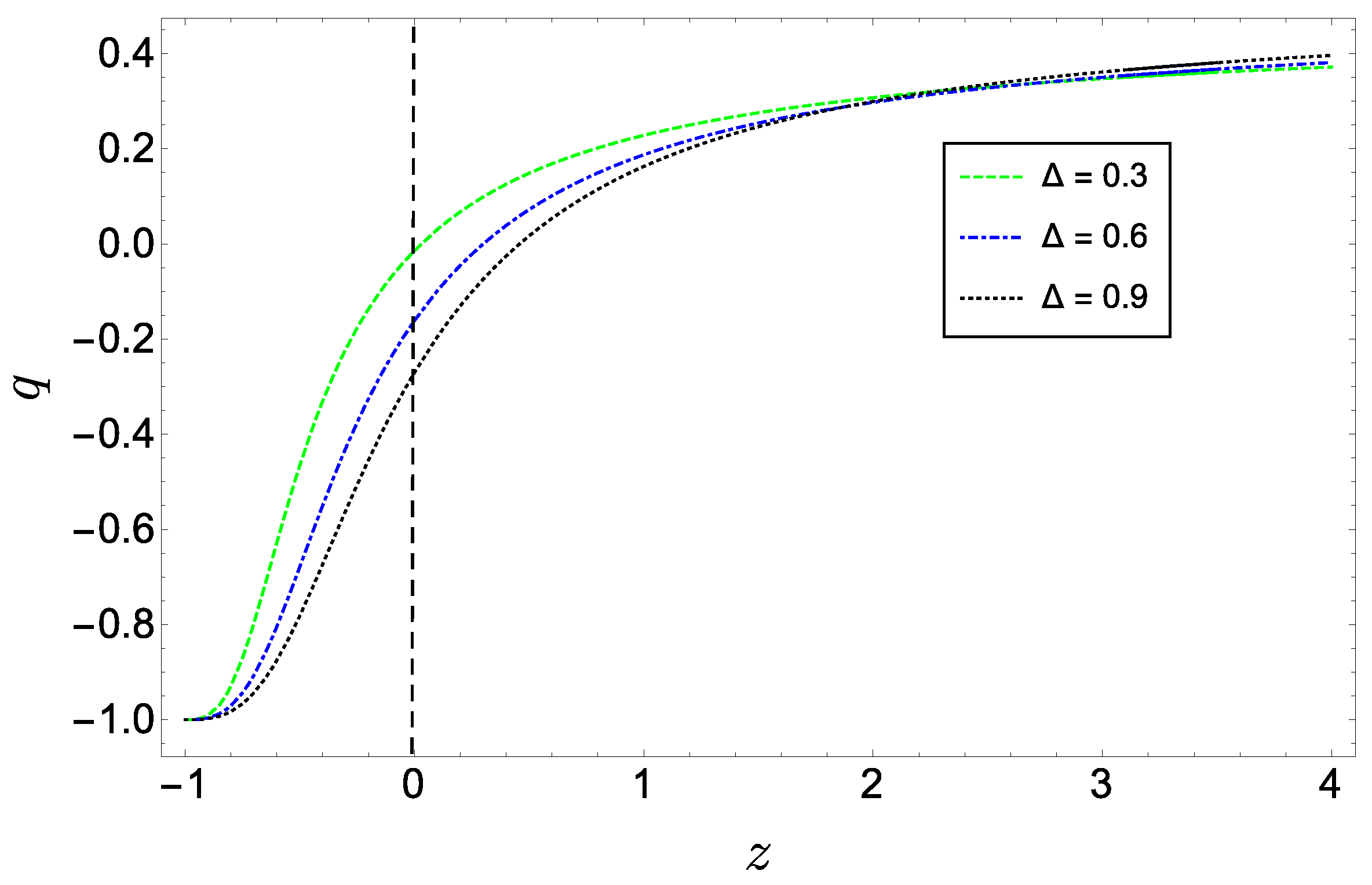
3. Tachyon Scalar Field as Barrow Holographic Dark Energy in a Non-Flat FRW Universe

In this Section we analyze the correspondence between the tachyon dark energy model and the BHDE scenario in a non-flat FRW universe. Toward this end, we recall that in [33] it has been shown that the energy density ρ T and pressure p T for the tachyon scalar field take the form
ρ T = V ( T ) 1 T ˙ 2 ,
p T = V ( T ) 1 T ˙ 2 ,
where V ( T ) is the tachyon potential energy. From these relations, we derive the equation of state parameter (EoS) for the tachyon as
ω T = p T / ρ T = T ˙ 2 1 ,
which will be later equated to the EoS parameter of BHDE in our reconstructed scenario. In fact, in the present naive picture, the question we ask ourselves is how BHDE would appear if one imposes that the evolution of its energy density can be described in terms of that of tachyon field. More rigorously, one should derive the scalar field equation by computing the variation of the action including the lagrangian (38) with respect to the tachyon field T and specializing the result to the metric in Equation (2). The ensuing expression of T ˙ could then be used to fix the dynamics of the model (and, in particular, the scale factor) by comparison with BHDE [91].
We also remind that the cosmological model based on the effective Lagrangian of tachyonic matter
L ( T ) = V ( T ) 1 T , μ T , μ ,
with V ( T ) = c o n s t . coincides with the Chaplygin gas model.
Let us explicitly explore the connection between BHDE and tachyon dark energy model. Toward this end, we consider the time derivative of BHDE (10) and use Equation (16) to obtain
ρ ˙ D = C ( Δ 2 ) L Δ 3 1 1 | k | cos n ( | k | x ) ,
where x R h / a . By means of the continuity Equation (29), this can be cast as
3 H ρ D ( 1 + ω D ) 3 b 2 H ( ρ m + ρ D ) = C ( Δ 2 ) L Δ 3 1 1 | k | cos n ( | k | x ) .
We can now resort to Equation (37) to obtain
3 H ρ D T ˙ 2 3 b 2 H ( ρ m + ρ D ) = C ( Δ 2 ) L Δ 3 1 1 | k | cos n ( | k | x ) ,
where we have made use of the required correspondence ω T = ω D , as explained above. This relation can be further manipulated by dividing both sides by 3 H ρ D and using Equation (20) to give
T ˙ 2 b 2 ( u + 1 ) = C ( Δ 2 ) L Δ 3 3 H ρ D 1 1 | k | cos n ( | k | x ) .
After employing Equation (10) and the condition L = H 1 , we finally reach
T ˙ 2 b 2 ( u + 1 ) = Δ 2 3 1 1 | k | cos n ( | k | x ) ,
which can be equivalently written as
T ˙ 2 = 2 3 b 2 ( u + 1 ) Δ 3 + Δ 2 3 1 k cos n ( | k | x ) .
Notice that, once known T ˙ 2 , one can express the tachyon potential V ( T ) in terms of H and the parameter Δ by simply equating Equations (10) and (35).
Let us now study the cases k = 0 , 1 , 1 separately. The k = 0 framework corresponds to a flat FRW universe. In this case it is easy to show that
T ˙ 2 = b 2 Ω D ,
where we have used Equations (17) and (20). Thus, if we require T ˙ to be real, then b = 0 in flat space, which allows us to conclude that T ˙ 2 must always be vanishing in flat space, independently of the existence of interaction. In turn, from Equations (35) and (36) this implies
ρ T = p T .
We conclude that in this case, the equation of state is always ω D = 1 , reproducing a cosmological constant-like behavior.
On the other hand, for k = 1 (closed FRW universe) we obtain from the definition (17)
T ˙ 2 = 2 3 b 2 ( u + 1 ) Δ 3 + Δ 2 3 cos ( x ) .
In order for T ˙ to be zero (i.e., ω T = 1 ), we must have
cos ( x ) = 3 b 2 ( u + 1 ) Δ 2 + 1 ,
which clearly admits non-trivial solution, since Δ < 1 . This provides the condition for which the tachyon model of BHDE reproduces the cosmological constant behavior in a closed FRW universe. By contrast, in [62] it is argued that T ˙ 2 cannot be zero in Tsallis holographic dark energy in a non-flat universe.
The evolution trajectory of T ˙ 2 in Equation (47) is plotted in Figure 1 for fixed b and u and various allowed Δ . One can see that T ˙ 2 decreases monotonically for increasing cos ( x ) and T ˙ 2 0 , so that ω T 1 (quintessence or cosmological constant-like behavior), while tending to negative values for c o s ( x ) 1 , which becomes physically invalid. The non-interacting case can be simply derived by setting b 2 = 0 in Equations (47) and (48). The ensuing behavior is similar to that described above, the only difference being that T ˙ 2 0 throughout the whole evolution in this case.
Similarly, we can consider the dynamics of the tachyon field in an open ( k = 1 ) universe. Following the same reasoning as above, we obtain
T ˙ 2 = 2 3 b 2 ( u + 1 ) Δ 3 + Δ 2 3 cosh ( x ) .
The evolution of T ˙ 2 in Equation (49) is plotted in Figure 2 for different values of Δ . As before, we notice that T ˙ 2 decreases monotonically for increasing cosh ( x ) , but in this case it is always negative, which is not a physically valid situation. We also see that Equation (49) vanishes, provided that
cosh ( x ) = 3 b 2 ( u + 1 ) Δ 2 + 1 .
However, since cosh ( x ) > 1 (we remind that x 0 ), we infer T ˙ 2 can never be zero, in agreement with the result of [62]. The same behavior is exhibited in the absence of interactions ( b 2 = 0 ).

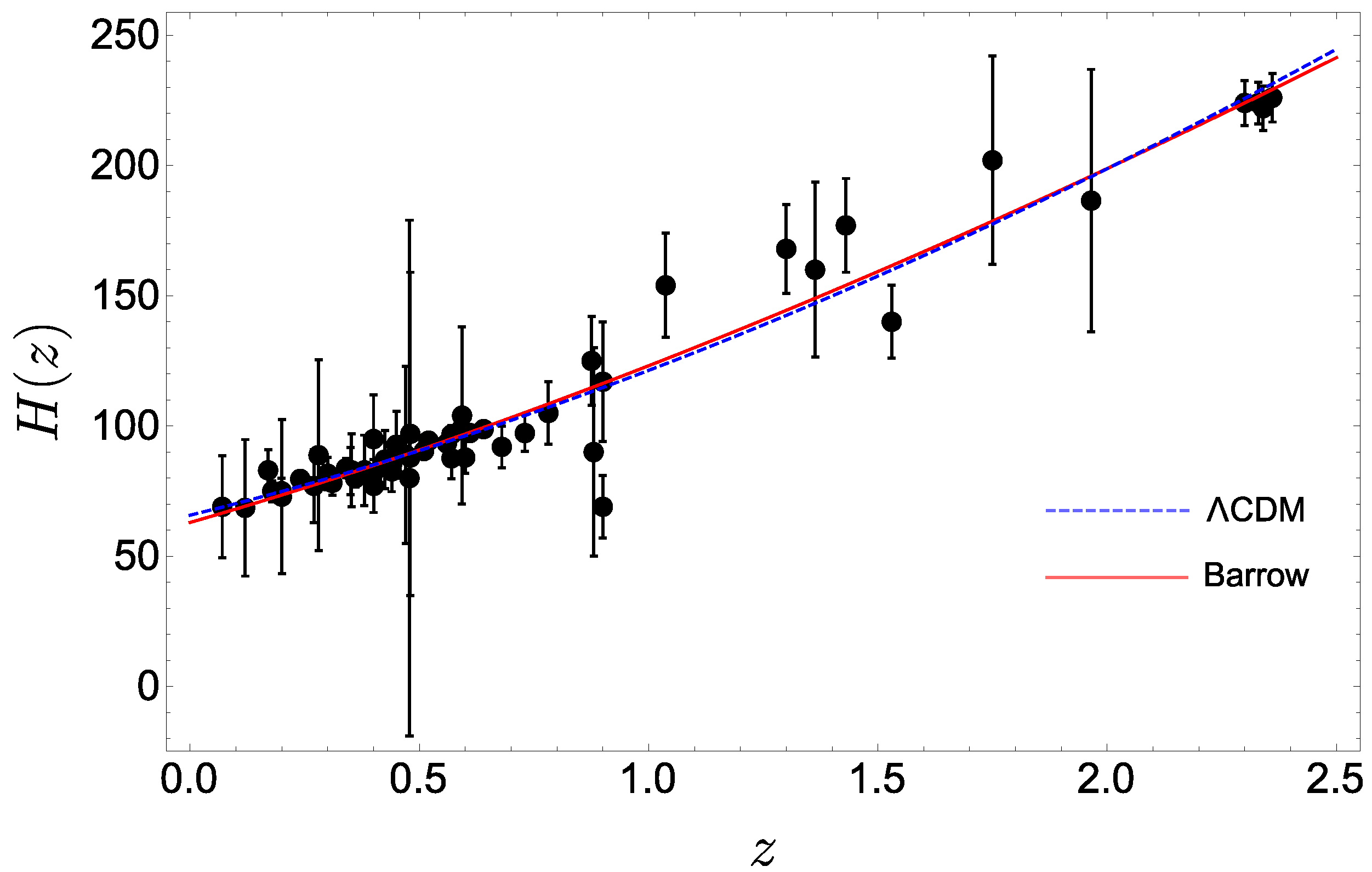
Observational Studies

This section is devoted to explore some observational implications of BHDE. For simplicity, we focus on the case where there is no interaction between the dark sectors of the cosmos and positive values of curvature. First, we notice that the use of Equation (23) in non-flat universe allows us to write down the deceleration parameter q as
q = a ¨ a H 2 = 1 H ˙ H 2 = 1 Ω k + 3 Ω D 2 1 + u + ω D .
From the above definition, one can check that q > 0 ( q < 0 ) corresponds to a decelerated (accelerated) expansion of the universe, since a ¨ < 0 ( a ¨ > 0 ). By computing the time derivative of Equation (10), we then get
ρ ˙ D = 2 Δ ρ D H Ω k 3 Ω D 2 1 + u + ω D ,
while the further usage of the definition (12) leads to
Ω D = Ω D 1 2 2 Δ 3 + Ω k + 3 Ω D ω D + 2 Ω k 3 Ω D 1 + u + ω D ] .
where Ω D d Ω D d ( log a ) . By plugging into (22), the BHDE EoS parameter and the fractional BHDE density take the form
ω D = 3 + Δ 2 1 Ω k + 3 3 1 + Δ 2 1 Ω D ,
Ω D = Ω D Δ 2 3 + Ω k 3 Ω D 1 + Δ 2 1 Ω D .
The latter equation is solved numerically and plotted in Figure 3, which shows a monotonic increasing of dark energy for decreasing redshift, implying a DE dominated universe in the far future. On the other hand, the evolution of the EoS parameter is displayed in Figure 4, which indicates that BHDE behaves like quintessence or (asymptotically) the cosmological constant, consistently with the discussion below Figure 2. Specifically, for the considered Δ ’s, we can see that the present value of this parameter lies in the range 0.7 ω D , 0 0.4 , which only slightly deviates from recent Planck+WP+BAO predictions [92].
Similarly, from Equation (51) we can derive the evolution of the deceleration parameter, whose behavior is plotted in Figure 5. We observe that the present model allows to explain the sequence of an early decelerating (i.e., q > 0 ) expansion of the universe, followed by an accelerated (i.e., q < 0 ) epoch. Additionally, it is consistent with the description of the current acceleration, although the predicted value 0.3 q 0 0.01 is slightly higher than q 0 0.5 obtained in the standard Λ CDM model [92].
To further investigate the phenomenological consistency of the present model, let us consider the evolution of the Hubble rate H ( z ) from Equations (51) and (55) for fixed Ω k = 0.01 and Ω D 0 = 0.73 , and compare it with the data points obtained from 57 Hubble’s parameter measurements in the range 0.07 z 2.36 . These data have been derived via Differential Age (31 points), BAO and other methods (the remaining 26 points) and are reported in Table 1 below.
We employ the statistical R 2 -test to find the best fit value of model parameters. This is given by
R 2 = 1 i = 1 57 ( H i ) o b ( H i ) t h 2 i = 1 57 ( H i ) o b ( H i ) m e a n 2 ,
where ( H i ) o b and ( H i ) t h are the observed and predicted values of Hubble rate, respectively. Requiring that the deviation of R 2 from unity is minimized gives the best-fit (mean) value Δ 0.09 , to be compared with other estimates of Barrow parameter found, for example, in [44,80,81,93].
The fit in Figure 6 also allows us to infer the current value of Hubble’s parameter predicted by our model, which is H 0 = ( 65.1 ± 5.8 ) km s 1 Mpc 1 . This is to compare with the recent observation from Planck Collaboration H 0 = 67.27 ± 0.60 km s 1 Mpc 1 [92]. Also, we remark that the major discrepancy between the prediction of our model and Λ CDM is observed at higher redshift, where Barrow (quantum gravitational-like) effects presumable become more appreciable.
Further observational study of our model can be conducted, for instance, by analyzing the cosmological distance modulus and the effects of the Barrow model on the growth of cosmological perturbations. These studies require further effort and will be presented in a future work.

4. Inflation in Barrow Holographic Dark Energy

In this Section we discuss inflation in BHDE (see also [94]). For reasons that will appear clear below and following [95], here we consider the more general expression for the length scale L 2 = α H 2 + β H ˙ , where α and β are dimensionless constant. Assuming that the expansion of the universe is driven by BHDE (10) and neglecting the matter contribution due to the rapid inflationary expansion, Equation (18) becomes
H 2 = C 3 M p 2 α H 2 + β H ˙ 1 Δ / 2 ,
from which we infer
H ˙ = H 2 β 3 M p 2 C 2 2 Δ ( H 2 ) Δ 2 Δ α .
From this relation, it is clear that setting the IR cutoff L H 1 (i.e., β = 0 ) as in the previous study would give rise to technical issues in the present framework.
To simplify the resolution of Equation (58), we introduce the e-folds variable N = log a / a i , where a i is the initial value of the scale factor a. By observing that d N = H d t and H ˙ = 1 2 d H 2 d N , integration of Equation (58) gives
log H ˜ 2 γ H ˜ 2 Δ 2 Δ 1 2 / Δ α | H ˜ i H ˜ f = 2 α N β ,
where H ˜ = H / M p is the dimensionless Hubble parameter and
γ = 3 M p 2 C 2 2 Δ M p 2 Δ 2 Δ .
Here, we have denoted the Hubble parameter at the end of inflation by H ˜ f .
From Equation (57) we can now compute the characteristic parameters of slow-roll inflation. Specifically, the first slow-roll parameter is given by
ϵ 1 = H ˙ H 2 = 1 β γ H ˜ 2 Δ 2 Δ α .
The other slow-roll parameters can be derived by using the definition ϵ n + 1 = d log ( ϵ n ) / d N . For the second parameter ϵ 2 we obtain
ϵ 2 = ϵ ˙ 1 H ϵ 1 = 2 γ β Δ 2 Δ H ˜ 2 Δ 2 Δ .
Let us now evaluate the Hubble parameter at the end of inflation. This phase is characterized by ϵ 1 = 1 . By straightforward calculations, we obtain
H ˜ f 2 = γ α β 1 2 / Δ .
On the other hand, at the beginning of inflation (including the horizon crossing time) Equation (59) gives
H ˜ i 2 = γ α 1 + β e 2 α N / β α β 1 2 / Δ ,
which can be used to calculate the slow-roll parameters for earlier time by direct substitution in Equations (61) and (62).
In order to derive the scalar spectral index n s 1 and the tensor-to-scalar ratio r, we follow [95,96] and make use of the usual perturbation procedure. We are led to
n s 1 = 2 ϵ 1 2 ϵ 2 , r = 16 ϵ 1 .
Clearly, a full perturbation analysis is needed to obtain the exact expressions of n s 1 and r.
Two comments are in order here: first, we notice that the constant γ does not intervene in the calculation of the slow-roll parameters at the horizon crossing time, which means that neither n s 1 nor r depend on it. As explained in [95], this constant can be estimated by considering the amplitude of the scalar perturbation. Furthermore, it is worth mentioning that a similar analysis of inflation and correspondence between BHDE and tachyon field has been proposed in [97]. However, in that case the authors consider values of Barrow parameter Δ higher than unity, which is actually forbidden in the Barrow model. This somehow questions the results exhibited in [97].

Trans-Planckian Censorship Conjecture

The large-scale structures we currently see in the universe originated from matter and energy quantum fluctuations produced during inflation. Such fluctuations cross the Hubble radius during the early phase, are stretched out and classicalize, and finally re-enter the Hubble horizon to produce the CMB anisotropies. The key point is that if inflation lasted longer than the supposed minimal period, then it would be possible to observe length scales originated from modes smaller than the Planck length at inflation [98]. This problem is usually referred to as “trans-Planckian problem”. To avoid inconsistencies, it has been conjectured that this problem cannot arise in any consistent model of quantum gravity (“trans-Planckian censorship conjecture”, TCC) [99].
The TCC states that no length scales which cross the Hubble horizon could ever have had a wavelength smaller than the Planck length. This is imposed by requiring that
L p a i < H f 1 a f ,
where L p = 1 / M p is the Planck length and we have denoted by a f the scale factor at the end of inflation. By using Equation (63) for the Hubble parameter at the final time, the TCC (66) becomes
γ α β 1 2 / Δ < ( 8 π e N ) 2 ,
the validity of which can be examined by comparison with observational data. This aspect is under active investigation and will be addressed in more detail in a future work.

5. Conclusions and Outlook

The origin of the accelerated expansion of the universe is an open problem in modern cosmology. To date, the most reliable explanation is provided by the existence of an enigmatic form of energy—dark energy—affecting the universe on large scales. Several candidates have been considered to account for this phenomenon. In particular, holographic dark energy has been largely studied, also in connection with different real scalar field theories, such as quintessence [3,4,5,6], K-essence [7], phantom [9,10,11], interacting models [16], and tachyon [33] (see also [100,101] for arguments that theoretically rule out quintessence and K-essence). Recently, the interest has been extended to the Tsallis holographic dark energy [43,44,47,48,49] and the possibility of using it to describe the dynamics of the tachyon field [62].
In this work we have considered the further scenario of tachyon model as Barrow holographic dark energy. Barrow entropy arises from the effort to include quantum gravity effects on the black hole horizon. In this sense, the present analysis must be intended as a preliminary step toward a fully quantum gravity extension of [62]. In the absence of empirical guidelines, we have exploited the powerful tool of Lagrangian formalism and, in perspective, the precious clues that may be provided by the related Noether’s theorem. In particular, we have established a correspondence between BHDE and the tachyon field model in a FRW universe, both in the presence and absence of interactions between dark energy and matter. In this regard, we would like to stress that the aim of the present analysis is to reconstruct BHDE in the tachyon model, rather than showing the consistency between the two frameworks. In other terms, in the absence of a Lagrangian formulation of BHDE, the question we have asked ourselves is how BHDE would appear if one requires that the evolution of its energy density can be described in terms of that of the tachyon field. As a result, we have shown that the tachyon field should exhibit non-trivial dynamics. In particular, in a flat universe, T ˙ 2 must always be vanishing, independently of the existence of interaction, which implies ω D = 1 for the equation-of-state parameter. On the other hand, for a non-flat universe and various values of Barrow parameters, we have found that T ˙ 2 decreases monotonically for increasing cos ( R h / a ) and cosh ( R h / a ) . Specifically, T ˙ 2 0 for a closed universe, while T ˙ 2 < 0 for an open one, which is physically not allowed. We have finally investigated an inflationary scenario described by a universe filled with BHDE and commented on the trans-Planckian censorship conjecture.
We have shown that the tachyon field exhibits a non-trivial dynamics. In a flat universe, T ˙ 2 must always be vanishing, independently of the existence of interaction, which implies ω D = 1 for the equation-of-state parameter. On the other hand, for a non-flat universe and various values of Barrow parameters, we have found that T ˙ 2 decreases monotonically for increasing cos ( R h / a ) and cosh ( R h / a ) . Specifically, T ˙ 2 0 for a closed universe, while T ˙ 2 < 0 for an open one, which is physically not allowed. We have finally discussed observational consistency of our model and investigated an inflationary scenario described by a universe filled with BHDE and commented on the trans-Planckian censorship conjecture.
Further aspects remain to be addressed. For instance, we can look at the correspondence between the tachyon field and other dark energy scenarios, in particular stable dark energy models. Furthermore, it would be interesting to disclose the effects of Barrow entropic corrections on the growth of perturbations and structure formation in the present model. Preliminary studies along this direction have been recently conducted in [102]. One more suggestive perspective concerns the extension of the above framework by using different IR cutoffs [26] (such as the future event horizon or Grand–Oliveros cutoff) and/or other deformed entropies, such as Kaniadakis entropy [49], which is based on a relativistic self-consistent generalization of the classical Boltzmann–Gibbs entropy [77] (see also [103] for a recent review of Kaniadakis entropy applications in gravity and cosmology). Finally, it is essential to examine to what extent our effective model reconciles with predictions of more fundamental candidate theories of quantum gravity, such as string theory and loop quantum gravity, or more phenomenological approaches, such as generalizations of the Heisenberg relation at Planck scale [104,105,106,107]. Work along these directions requires further investigation and will be presented elsewhere.

Author Contributions

Conceptualization, investigation, methodology, validation, supervision, writing and original draft preparation, G.G.L. Methodology, reading, Y.L. All authors have read and agreed to the published version of the manuscript.

Funding

This research received no external funding.

Data Availability Statement

Data sharing is not applicable to this article as no datasets were generated or analyzed during the current study.

Acknowledgments

The authors are grateful to the anonymous referees for their comments, which helped to improve the quality of the manuscript. G.G.L. acknowledges the Spanish “Ministerio de Universidades” for the awarded Maria Zambrano fellowship and funding received from the European Union—NextGenerationEU. He also acknowledges participation in the COST Association Action CA18108 “Quantum Gravity Phenomenology in the Multimessenger Approach” and LISA Cosmology Working group. He is finally grateful to Pasquale Bosso for technical suggestions on the final editing of the manuscript.

Conflicts of Interest

The authors declare no conflict of interest.

Abbreviations

The following abbreviations are used in this manuscript:
HDEHolographic Dark Energy
BHDEBarrow Holographic Dark Energy

References

  1. Sahni, V.; Starobinsky, A.A. The Case for a positive cosmological Lambda term. Int. J. Mod. Phys. D 2000, 9, 373–444. [Google Scholar] [CrossRef]
  2. Peebles, P.J.E.; Ratra, B. The Cosmological Constant and Dark Energy. Rev. Mod. Phys. 2003, 75, 559–606. [Google Scholar] [CrossRef]
  3. Ratra, B.; Peebles, P.J.E. Cosmological Consequences of a Rolling Homogeneous Scalar Field. Phys. Rev. D 1988, 37, 3406. [Google Scholar] [CrossRef] [PubMed]
  4. Frieman, J.A.; Hill, C.T.; Stebbins, A.; Waga, I. Cosmology with ultralight pseudo Nambu-Goldstone bosons. Phys. Rev. Lett. 1995, 75, 2077–2080. [Google Scholar] [CrossRef]
  5. Turner, M.S.; White, M.J. CDM models with a smooth component. Phys. Rev. D 1997, 56, R4439. [Google Scholar] [CrossRef]
  6. Caldwell, R.R.; Dave, R.; Steinhardt, P.J. Cosmological imprint of an energy component with general equation of state. Phys. Rev. Lett. 1998, 80, 1582–1585. [Google Scholar] [CrossRef]
  7. Armendariz-Picon, C.; Mukhanov, V.F.; Steinhardt, P.J. A Dynamical solution to the problem of a small cosmological constant and late time cosmic acceleration. Phys. Rev. Lett. 2000, 85, 4438–4441. [Google Scholar] [CrossRef]
  8. Armendariz-Picon, C.; Mukhanov, V.F.; Steinhardt, P.J. Essentials of k essence. Phys. Rev. D 2001, 63, 103510. [Google Scholar] [CrossRef]
  9. Caldwell, R.R. A Phantom menace? Phys. Lett. B 2002, 545, 23–29. [Google Scholar] [CrossRef]
  10. Caldwell, R.R.; Kamionkowski, M.; Weinberg, N.N. Phantom energy and cosmic doomsday. Phys. Rev. Lett. 2003, 91, 071301. [Google Scholar] [CrossRef]
  11. Nojiri, S.; Odintsov, S.D. Quantum de Sitter cosmology and phantom matter. Phys. Lett. B 2003, 562, 147–152. [Google Scholar] [CrossRef]
  12. Feng, B.; Wang, X.L.; Zhang, X.M. Dark energy constraints from the cosmic age and supernova. Phys. Lett. B 2005, 607, 35–41. [Google Scholar] [CrossRef]
  13. Guo, Z.K.; Piao, Y.S.; Zhang, X.M.; Zhang, Y.Z. Cosmological evolution of a quintom model of dark energy. Phys. Lett. B 2005, 608, 177–182. [Google Scholar] [CrossRef]
  14. Elizalde, E.; Nojiri, S.; Odintsov, S.D. Late-time cosmology in (phantom) scalar-tensor theory: Dark energy and the cosmic speed-up. Phys. Rev. D 2004, 70, 043539. [Google Scholar] [CrossRef]
  15. Nojiri, S.; Odintsov, S.D.; Tsujikawa, S. Properties of singularities in (phantom) dark energy universe. Phys. Rev. D 2005, 71, 063004. [Google Scholar] [CrossRef]
  16. Deffayet, C.; Dvali, G.R.; Gabadadze, G. Accelerated universe from gravity leaking to extra dimensions. Phys. Rev. D 2002, 65, 044023. [Google Scholar] [CrossRef]
  17. D’Agostino, R. Holographic dark energy from nonadditive entropy: Cosmological perturbations and observational constraints. Phys. Rev. D 2019, 99, 103524. [Google Scholar] [CrossRef]
  18. Capozziello, S.; D’Agostino, R. A cosmographic outlook on dark energy and modified gravity. arXiv 2022, arXiv:2211.17194. [Google Scholar]
  19. Capolupo, A.; Quaranta, A. Neutrino capture on tritium as a probe of flavor vacuum condensate and dark matter. Phys. Lett. B 2023, 839, 137776. [Google Scholar] [CrossRef]
  20. Capolupo, A.; Quaranta, A. Boson mixing and flavor vacuum in the expanding Universe: A possible candidate for the dark energy. Phys. Lett. B 2023, 840, 137889. [Google Scholar] [CrossRef]
  21. Lambiase, G.; Mishra, H.; Mohanty, S. Dark energy from Neutrinos and Standard Model Higgs potential. Astropart. Phys. 2012, 35, 629–633. [Google Scholar] [CrossRef]
  22. Lambiase, G.; Mohanty, S.; Narang, A.; Parashari, P. Testing dark energy models in the light of σ8 tension. Eur. Phys. J. C 2019, 79, 141. [Google Scholar] [CrossRef]
  23. Cohen, A.G.; Kaplan, D.B.; Nelson, A.E. Effective field theory, black holes, and the cosmological constant. Phys. Rev. Lett. 1999, 82, 4971–4974. [Google Scholar] [CrossRef]
  24. Horava, P.; Minic, D. Probable values of the cosmological constant in a holographic theory. Phys. Rev. Lett. 2000, 85, 1610–1613. [Google Scholar] [CrossRef] [PubMed]
  25. Thomas, S.D. Holography stabilizes the vacuum energy. Phys. Rev. Lett. 2002, 89, 081301. [Google Scholar] [CrossRef] [PubMed]
  26. Li, M. A Model of holographic dark energy. Phys. Lett. B 2004, 603, 1. [Google Scholar] [CrossRef]
  27. Bamba, K.; Capozziello, S.; Nojiri, S.; Odintsov, S.D. Dark energy cosmology: The equivalent description via different theoretical models and cosmography tests. Astrophys. Space Sci. 2012, 342, 155–228. [Google Scholar] [CrossRef]
  28. Ghaffari, S.; Dehghani, M.H.; Sheykhi, A. Holographic dark energy in the DGP braneworld with Granda-Oliveros cutoff. Phys. Rev. D 2014, 89, 123009. [Google Scholar] [CrossRef]
  29. Wang, S.; Wang, Y.; Li, M. Holographic Dark Energy. Phys. Rep. 2017, 696, 1–57. [Google Scholar] [CrossRef]
  30. ’t Hooft, G. Dimensional reduction in quantum gravity. Conf. Proc. C 1993, 930308, 284–296. [Google Scholar]
  31. Susskind, L. The World as a hologram. J. Math. Phys. 1995, 36, 6377–6396. [Google Scholar] [CrossRef]
  32. Enqvist, K.; Hannestad, S.; Sloth, M.S. Searching for a holographic connection between dark energy and the low-l CMB multipoles. JCAP 2005, 02, 004. [Google Scholar] [CrossRef]
  33. Setare, M.R. Holographic tachyon model of dark energy. Phys. Lett. B 2007, 653, 116–121. [Google Scholar] [CrossRef]
  34. Hsu, S.D.H. Entropy bounds and dark energy. Phys. Lett. B 2004, 594, 13–16. [Google Scholar] [CrossRef]
  35. Srivastava, S.; Sharma, U.K. Barrow holographic dark energy with Hubble horizon as IR cutoff. Int. J. Geom. Meth. Mod. Phys. 2021, 18, 2150014. [Google Scholar] [CrossRef]
  36. Gong, Y.G. Holographic bound in Brans-Dicke cosmology. Phys. Rev. D 2000, 61, 043505. [Google Scholar] [CrossRef]
  37. Kim, H.; Lee, H.W.; Myung, Y.S. Role of the Brans-Dicke scalar in the holographic description of dark energy. Phys. Lett. B 2005, 628, 11–17. [Google Scholar] [CrossRef]
  38. Nojiri, S.; Odintsov, S.D. Unifying phantom inflation with late-time acceleration: Scalar phantom-non-phantom transition model and generalized holographic dark energy. Gen. Relativ. Gravit. 2006, 38, 1285–1304. [Google Scholar] [CrossRef]
  39. Setare, M.R. The Holographic dark energy in non-flat Brans-Dicke cosmology. Phys. Lett. B 2007, 644, 99–103. [Google Scholar] [CrossRef]
  40. Banerjee, N.; Pavon, D. A Quintessence scalar field in Brans-Dicke theory. Class. Quant. Grav. 2001, 18, 593. [Google Scholar] [CrossRef]
  41. Xu, L.; Lu, J. Holographic Dark Energy in Brans-Dicke Theory. Eur. Phys. J. C 2009, 60, 135–140. [Google Scholar] [CrossRef]
  42. Khodam-Mohammadi, A.; Karimkhani, E.; Sheykhi, A. Best values of parameters for interacting HDE with GO IR-cutoff in Brans–Dicke cosmology. Int. J. Mod. Phys. D 2014, 23, 1450081. [Google Scholar] [CrossRef]
  43. Tavayef, M.; Sheykhi, A.; Bamba, K.; Moradpour, H. Tsallis Holographic Dark Energy. Phys. Lett. B 2018, 781, 195–200. [Google Scholar] [CrossRef]
  44. Saridakis, E.N.; Bamba, K.; Myrzakulov, R.; Anagnostopoulos, F.K. Holographic dark energy through Tsallis entropy. JCAP 2018, 12, 012. [Google Scholar] [CrossRef]
  45. Nojiri, S.; Odintsov, S.D.; Saridakis, E.N. Modified cosmology from extended entropy with varying exponent. Eur. Phys. J. C 2019, 79, 242. [Google Scholar] [CrossRef]
  46. Luciano, G.G.; Gine, J. Baryogenesis in non-extensive Tsallis Cosmology. Phys. Lett. B 2022, 833, 137352. [Google Scholar] [CrossRef]
  47. Saridakis, E.N. Barrow holographic dark energy. Phys. Rev. D 2020, 102, 123525. [Google Scholar] [CrossRef]
  48. Moradpour, H.; Ziaie, A.H.; Kord Zangeneh, M. Generalized entropies and corresponding holographic dark energy models. Eur. Phys. J. C 2020, 80, 732. [Google Scholar] [CrossRef]
  49. Drepanou, N.; Lymperis, A.; Saridakis, E.N.; Yesmakhanova, K. Kaniadakis holographic dark energy and cosmology. Eur. Phys. J. C 2022, 82, 449. [Google Scholar] [CrossRef]
  50. Hernández-Almada, A.; Leon, G.; Magaña, J.; García-Aspeitia, M.A.; Motta, V.; Saridakis, E.N.; Yesmakhanova, K. Kaniadakis-holographic dark energy: Observational constraints and global dynamics. Mon. Not. R. Astron. Soc. 2022, 511, 4147–4158. [Google Scholar] [CrossRef]
  51. Nojiri, S.; Odintsov, S.D.; Paul, T. Barrow entropic dark energy: A member of generalized holographic dark energy family. Phys. Lett. B 2022, 825, 136844. [Google Scholar] [CrossRef]
  52. Luciano, G.G. Modified Friedmann equations from Kaniadakis entropy and cosmological implications on baryogenesis and 7Li-abundance. Eur. Phys. J. C 2022, 82, 314. [Google Scholar] [CrossRef]
  53. Ghaffari, S.; Luciano, G.G.; Capozziello, S. Barrow holographic dark energy in the Brans–Dicke cosmology. Eur. Phys. J. Plus 2023, 138, 82. [Google Scholar] [CrossRef]
  54. Nojiri, S.; Odintsov, S.D.; Faraoni, V. From nonextensive statistics and black hole entropy to the holographic dark universe. Phys. Rev. D 2022, 105, 044042. [Google Scholar] [CrossRef]
  55. Nojiri, S.; Odintsov, S.D.; Paul, T. Early and late universe holographic cosmology from a new generalized entropy. Phys. Lett. B 2022, 831, 137189. [Google Scholar] [CrossRef]
  56. Luciano, G.G. Cosmic evolution and thermal stability of Barrow holographic dark energy in a nonflat Friedmann-Robertson-Walker Universe. Phys. Rev. D 2022, 106, 083530. [Google Scholar] [CrossRef]
  57. Luciano, G.G.; Giné, J. Generalized interacting Barrow Holographic Dark Energy: Cosmological predictions and thermodynamic considerations. arXiv 2022, arXiv:2210.09755. [Google Scholar]
  58. Luciano, G.G. From the emergence of cosmic space to horizon thermodynamics in Barrow entropy-based Cosmology. Phys. Lett. B 2023, 838, 137721. [Google Scholar] [CrossRef]
  59. Nojiri, S.; Odintsov, S.D.; Saridakis, E.N.; Myrzakulov, R. Correspondence of cosmology from non-extensive thermodynamics with fluids of generalized equation of state. Nucl. Phys. B 2020, 950, 114850. [Google Scholar] [CrossRef]
  60. Bajardi, F.; Capozziello, S. Noether symmetries and quantum cosmology in extended teleparallel gravity. Int. J. Geom. Meth. Mod. Phys. 2021, 18, 2140002. [Google Scholar] [CrossRef]
  61. Acunzo, A.; Bajardi, F.; Capozziello, S. Non-local curvature gravity cosmology via Noether symmetries. Phys. Lett. B 2022, 826, 136907. [Google Scholar] [CrossRef]
  62. Liu, Y. Tachyon model of Tsallis holographic dark energy. Eur. Phys. J. Plus 2021, 136, 579. [Google Scholar] [CrossRef]
  63. Gibbons, G.W. Cosmological evolution of the rolling tachyon. Phys. Lett. B 2002, 537, 1–4. [Google Scholar] [CrossRef]
  64. Mazumdar, A.; Panda, S.; Perez-Lorenzana, A. Assisted inflation via tachyon condensation. Nucl. Phys. B 2001, 614, 101–116. [Google Scholar] [CrossRef]
  65. Padmanabhan, T. Accelerated expansion of the universe driven by tachyonic matter. Phys. Rev. D 2002, 66, 021301. [Google Scholar] [CrossRef]
  66. Ens, P.S.; Santos, A.F. f (R) gravity and Tsallis holographic dark energy. EPL 2020, 131, 40007. [Google Scholar] [CrossRef]
  67. Zubair, M.; Durrani, L.R. Exploring tsallis holographic dark energy scenario in f (R, T) gravity. Chin. J. Phys. 2021, 69, 153–171. [Google Scholar] [CrossRef]
  68. Sharif, M.; Saba, S. Tsallis Holographic Dark Energy in f (G, T) Gravity. Symmetry 2019, 11, 92. [Google Scholar] [CrossRef]
  69. Waheed, S. Reconstruction paradigm in a class of extended teleparallel theories using Tsallis holographic dark energy. Eur. Phys. J. Plus 2020, 135, 11. [Google Scholar] [CrossRef]
  70. Ghaffari, S.; Moradpour, H.; Lobo, I.P.; Morais Graça, J.P.; Bezerra, V.B. Tsallis holographic dark energy in the Brans–Dicke cosmology. Eur. Phys. J. C 2018, 78, 706. [Google Scholar] [CrossRef]
  71. Aditya, Y.; Mandal, S.; Sahoo, P.K.; Reddy, D.R.K. Observational constraint on interacting Tsallis holographic dark energy in logarithmic Brans–Dicke theory. Eur. Phys. J. C 2019, 79, 1020. [Google Scholar] [CrossRef]
  72. Sobhanbabu, Y.; Vijaya Santhi, M. Kantowski–Sachs Tsallis holographic dark energy model with sign-changeable interaction. Eur. Phys. J. C 2021, 81, 1040. [Google Scholar] [CrossRef]
  73. Luciano, G.G. Saez-Ballester gravity in Kantowski-Sachs Universe: A new reconstruction paradigm for Barrow Holographic Dark Energy. Phys. Dark Universe 2023, 41, 101237. [Google Scholar] [CrossRef]
  74. Barrow, J.D. The Area of a Rough Black Hole. Phys. Lett. B 2020, 808, 135643. [Google Scholar] [CrossRef]
  75. Tsallis, C. Possible Generalization of Boltzmann-Gibbs Statistics. J. Stat. Phys. 1988, 52, 479–487. [Google Scholar] [CrossRef]
  76. Tsallis, C.; Cirto, L.J.L. Black hole thermodynamical entropy. Eur. Phys. J. C 2013, 73, 2487. [Google Scholar] [CrossRef]
  77. Kaniadakis, G. Statistical mechanics in the context of special relativity. Phys. Rev. E 2002, 66, 056125. [Google Scholar] [CrossRef]
  78. Luciano, G.G.; Blasone, M. q-generalized Tsallis thermostatistics in Unruh effect for mixed fields. Phys. Rev. D 2021, 104, 045004. [Google Scholar] [CrossRef]
  79. Luciano, G.G.; Blasone, M. Nonextensive Tsallis statistics in Unruh effect for Dirac neutrinos. Eur. Phys. J. C 2021, 81, 995. [Google Scholar] [CrossRef]
  80. Barrow, J.D.; Basilakos, S.; Saridakis, E.N. Big Bang Nucleosynthesis constraints on Barrow entropy. Phys. Lett. B 2021, 815, 136134. [Google Scholar] [CrossRef]
  81. Luciano, G.G.; Saridakis, E.N. Baryon asymmetry from Barrow entropy: Theoretical predictions and observational constraints. Eur. Phys. J. C 2022, 82, 558. [Google Scholar] [CrossRef]
  82. Vagnozzi, S.; Roy, R.; Tsai, Y.D.; Visinelli, L. Horizon-scale tests of gravity theories and fundamental physics from the Event Horizon Telescope image of Sagittarius A*. arXiv 2022, arXiv:2205.07787. [Google Scholar]
  83. Di Gennaro, S.; Ong, Y.C. Sign Switching Dark Energy from a Running Barrow Entropy. Universe 2022, 8, 541. [Google Scholar] [CrossRef]
  84. Guberina, B.; Horvat, R.; Nikolic, H. Nonsaturated Holographic Dark Energy. JCAP 2007, 01, 012. [Google Scholar] [CrossRef]
  85. Sheykhi, A.; Hamedan, M.S. Holographic dark energy in modified Barrow cosmology. Entropy 2023, 25, 569. [Google Scholar] [CrossRef]
  86. Al Mamon, A.; Mishra, A.K.; Sharma, U.K. Barrow Holographic dark energy in fractal cosmology. Int. J. Geom. Meth. Mod. Phys. 2022, 19, 2250231. [Google Scholar] [CrossRef]
  87. Ghaffari, S.; Sheykhi, A.; Dehghani, M.H. Statefinder diagnosis for holographic dark energy in the DGP braneworld. Phys. Rev. D 2015, 91, 023007. [Google Scholar] [CrossRef]
  88. Sheykhi, A. Holographic Scalar Fields Models of Dark Energy. Phys. Rev. D 2011, 84, 107302. [Google Scholar] [CrossRef]
  89. Boulkaboul, N. Baryogenesis triggered by Barrow holographic dark energy coupling. Phys. Dark Univ. 2023, 40, 101205. [Google Scholar] [CrossRef]
  90. Granda, L.N.; Oliveros, A. Infrared cut-off proposal for the Holographic density. Phys. Lett. B 2008, 669, 275–277. [Google Scholar] [CrossRef]
  91. Frolov, A.V.; Kofman, L.; Starobinsky, A.A. Prospects and problems of tachyon matter cosmology. Phys. Lett. B 2002, 545, 8–16. [Google Scholar] [CrossRef]
  92. Aghanim, N.; Akrami, Y.; Ashdown, M.; Aumont, J.; Baccigalupi, C.; Ballardini, M.; Banday, A.J.; Barreiro, R.B.; Bartolo, N.; Basak, S.; et al. Planck 2018 results. VI. Cosmological parameters. Astron. Astrophys. 2020, 641, A6, Erratum in Astron. Astrophys. 2021, 652, C4. [Google Scholar] [CrossRef]
  93. Anagnostopoulos, F.K.; Basilakos, S.; Saridakis, E.N. Observational constraints on Barrow holographic dark energy. Eur. Phys. J. C 2020, 80, 826. [Google Scholar] [CrossRef]
  94. Luciano, G.G. Constraining barrow entropy-based cosmology with power-law inflation. Eur. Phys. J. C 2023, 83, 329. [Google Scholar] [CrossRef]
  95. Mohammadi, A.; Golanbari, T.; Bamba, K.; Lobo, I.P. Tsallis holographic dark energy for inflation. Phys. Rev. D 2021, 103, 083505. [Google Scholar] [CrossRef]
  96. Nojiri, S.; Odintsov, S.D.; Saridakis, E.N. Holographic inflation. Phys. Lett. B 2019, 797, 134829. [Google Scholar] [CrossRef]
  97. Maity, S.; Rudra, P. Inflation driven by Barrow holographic dark energy. JHAP 2022, 2, 1–12. [Google Scholar] [CrossRef]
  98. Martin, J.; Brandenberger, R.H. The TransPlanckian problem of inflationary cosmology. Phys. Rev. D 2001, 63, 123501. [Google Scholar] [CrossRef]
  99. Bedroya, A.; Vafa, C. Trans-Planckian Censorship and the Swampland. JHEP 2020, 09, 123. [Google Scholar] [CrossRef]
  100. Banerjee, A.; Cai, H.; Heisenberg, L.; Colgáin, E.O.; Sheikh-Jabbari, M.M.; Yang, T. Hubble sinks in the low-redshift swampland. Phys. Rev. D 2021, 103, L081305. [Google Scholar] [CrossRef]
  101. Lee, B.H.; Lee, W.; Colgáin, E.O.; Sheikh-Jabbari, M.M.; Thakur, S. Is local H 0 at odds with dark energy EFT? JCAP 2022, 04, 004. [Google Scholar] [CrossRef]
  102. Sheykhi, A.; Farsi, B. Growth of perturbations in Tsallis and Barrow cosmology. Eur. Phys. J. C 2022, 82, 1111. [Google Scholar] [CrossRef]
  103. Luciano, G.G. Gravity and Cosmology in Kaniadakis Statistics: Current Status and Future Challenges. Entropy 2022, 24, 1712. [Google Scholar] [CrossRef]
  104. Kempf, A.; Mangano, G.; Mann, R.B. Hilbert space representation of the minimal length uncertainty relation. Phys. Rev. D 1995, 52, 1108–1118. [Google Scholar] [CrossRef]
  105. Scardigli, F. Generalized uncertainty principle in quantum gravity from micro-black hole Gedanken experiment. Phys. Lett. B 1999, 452, 39–44. [Google Scholar] [CrossRef]
  106. Bosso, P.; Das, S. Generalized ladder operators for the perturbed harmonic oscillator. Ann. Phys. 2018, 396, 254–265. [Google Scholar] [CrossRef]
  107. Luciano, G.G.; Petruzziello, L. Generalized uncertainty principle and its implications on geometric phases in quantum mechanics. Eur. Phys. J. Plus 2021, 136, 179. [Google Scholar] [CrossRef]
Figure 1. Evolution trajectories of T ˙ 2 for a closed ( k = 1 ) universe. We set u = 0.04 and b 2 = 0.01 as in [62].
Symmetry 15 01129 g001
Figure 2. Evolution trajectories of T ˙ 2 for an open ( k = 1 ) universe. We set u = 0.04 and b 2 = 0.01 as in [62].
Symmetry 15 01129 g002
Figure 3. Evolution trajectories of Ω D versus z (we set Ω k = 0.01 and Ω D 0 = 0.73 ). The dashed vertical line marks the value at present time.
Symmetry 15 01129 g003
Figure 4. Evolution trajectories of ω D versus z (we considered the same initial conditions as in Figure 3). The dashed vertical line marks the value at present time.
Symmetry 15 01129 g004
Figure 5. Evolution trajectories of q versus z (we considered the same initial conditions as in Figure 3). The dashed vertical line marks the value at present time.
Symmetry 15 01129 g005
Figure 6. Evolution of Hubble rate versus z. The black points are the observational data in Tab. Table 1, while the red solid (blue dashed) line is the best fit according to our model ( Λ CDM).
Symmetry 15 01129 g006
Table 1. 57 experimental points of H ( z ) (H is expressed in km s 1 Mpc 1 and σ H represents the uncertainty for each data point).
z H ( z ) σ H z H ( z ) σ H
0.07069.019.60.47838099
0.9069120.4809762
0.12068.626.20.59310413
0.1708380.6797928
0.17917540.781210512
0.19937550.875412517
0.20072.929.60.8809040
0.27077140.90011723
0.28088.836.61.03715420
0.351983141.30016817
0.380283.013.51.363160.033.6
0.40095171.43017718
0.400477.010.21.53014014
0.424787.111.21.75020240
0.449792.812.91.965186.550.4
0.4708934
0.2479.692.990.5294.352.64
0.3081.706.220.5693.342.30
0.3178.184.740.5787.67.8
0.3483.803.660.5796.83.4
0.3582.79.10.5998.483.18
0.3679.943.380.6087.96.1
0.3881.51.90.6197.32.1
0.4082.042.030.6498.822.98
0.4386.453.970.7397.37.0
0.4482.67.82.30224.08.6
0.4484.811.832.332248
0.4887.902.032.34222.08.5
0.5190.41.92.36226.09.3
Disclaimer/Publisher’s Note: The statements, opinions and data contained in all publications are solely those of the individual author(s) and contributor(s) and not of MDPI and/or the editor(s). MDPI and/or the editor(s) disclaim responsibility for any injury to people or property resulting from any ideas, methods, instructions or products referred to in the content.

