Parametric Symmetries in Architectures Involving Indefinite Causal Order and Path Superposition for Quantum Parameter Estimation of Pauli Channels

Abstract

Parameter estimation for devices containing or supporting quantum systems is a field of quantum metrology using quantum probe states to reach their characterization. Pauli channels are ideal structures where qubits are transmitted or contained, commonly altering them with specific fingerprints. The ultimate limit imposed on such estimation is addressed using the quantum Fisher information, stating a lower bound for it. Although the most simple scheme suggests performing such an estimation directly using the individual channel, other approaches have shown improved outcomes by repeating identical copies of the channel for the characterization, or otherwise those connected inside of specific circuit arrangements. These connections commonly include path superposition or causal indefinite architectures. In addition, other improvements have been observed in concrete channels when complementary unitary controls are included. The current research analyses the complete set of Pauli channels under some of those architectures in a comparative approach to reach a better estimation, thus stating hierarchies. It is observed that the use of those unitary controls notably improves previous outcomes by several orders of magnitude.

1. Introduction

Quantum systems are commonly characterized by parameters settling their structure. Such parameters drive their interactions with other external systems. In this process, the information depicting their evolution exhibits features inherited from such interactions and parameters. Thus, any kind of intermediate measurement should contain, in a greater or lesser degree, information about those parameters [1]. Then, the knowledge about those parameters becomes useful for characterising each channel, thus predicting its behaviour [2].

Classical Fisher information is a statistical function comprising information involved during a stochastic process [3]. It is then able to depict the information available to characterise the parameters driving such a process. A quantum approach to Fisher information is possible departing from the global density matrix of a specific system upon its interaction with the external environment under study. Then, Quantum Fisher information (QFI) can state a bound for the estimation of parameters belonging to that system or environment involved in the interaction [4].

In fact, the Cramér–Rao Bound (CRB) [5,6] involves Fisher information (classical or quantum) to set a limit for the variance associated with the quantum parameter estimation using those processes. This bound assumes the existence of a set of parameters $\left\{{\alpha }_i\right\}$ characterising the system, the environment, and/or their interaction, which could, in principle, be estimated through the statistical measurement of a set of observables $\left\{X_j\right\}$ fulfilling certain statistical distributions. Such a process is called quantum parameter estimation (QPE).

In particular, we are interested in the characterization of quantum channels. If fact, a quantum channel could be understood as an operation performed on a quantum state ${\rho }_{\mathrm{in}}$. A set of parameters $\left\{{\alpha }_i\right\}$ characterizes such an operation modifying the initial state ${\rho }_{\mathrm{in}}$ of the target system into ${\rho }_{\mathrm{out}}$ as an outcome. A quantum channel could then represent a medium or an environment where the quantum system remains or moves on. Then, those parameters characterise the effect of each specific channel on a quantum probe state ${\rho }_{\mathrm{i}\mathrm{n}}$, being transformed into ${\rho }_{\mathrm{out}}$. Such a transformation carries out information coming from the $\left\{{\alpha }_i\right\}$ parameters. The process is illustrated in Figure 1.

Even when a single channel could be directly analysed in terms of Figure 1, we could try to improve the last deployment by using scaffolding architectures where the analysed channel becomes immersed. That immersion has been proposed to construct more complex circuits in terms of sets of more simple circuits connected among them [7]. Such architectures could combine several identical channels to reinforce the information storage of the parameters from the single channel to be extracted through a convenient quantum probe state. Thus, sequential combinations, superposition channel paths, and even indefinite causal order (ICO) [8] have been considered in the quest for the best QPE processes [9,10].

Although ICO has demonstrated a higher efficiency in the improvement of communication processes (commonly analysed for the depolarising channel) [11], it could be an undesired effect because for QPE purposes, some noisier effects could be preferred to imprint a deeper fingerprint from the channel. Other practical alternatives have been tried in terms of channel architectures. These circuits involve copies of the analysed channels combined with complementary gates, such as unitary operations [12].

Regarding specific channels, a particular interest is in the simpler family of channels for qubits, the Pauli channels. Although Pauli channels could be generalised to higher dimensions, they are commonly intended for qubits, the most basic and spread quantum states in quantum processing and communication. In the current approach, quantum parameters estimation is analysed for the entire family of the two-dimensional Pauli channels. In fact, Pauli channels have already been analysed in terms of the QFI in QPE, but only using concrete channels implemented directly in the estimation procedure [13]. The QPE problem has also been analysed in the relativistic quantum processing arena by considering the Unhru effect framework. Thus, noisy channels on an accelerated qubit–qutrit system have analysed the QFI, particularly the maximum/minimum bounds of the parameter estimation [14,15,16]. In other approaches, stochastic procedures using entangled measurements provide an exponential advantage in quantum benchmarking [17] for Pauli channel estimation implementing entangled steering procedures [18].

Furthermore, Pauli channels have been analysed in general for the QPE problem, but only using redundant applications of the direct channels or alternatively ICO arrangements [9]. Thus, in previous work, it was settled that the advantage of ICO strategies becomes limited as compared with sequential application in the estimation strategy. Differently from the approach followed in [9], in this study, the analysis goes around the implementation of more elaborated circuits involving copies of a concrete but arbitrary Pauli channel, assisted by local unitary operations. This approach also considers path superposition together with sequential and ICO arrangements. As in [9], the use of a control system allows for a stochastic steering procedure as in [18]. As the single crossing of the quantum state on each type of channel could still be insufficient to efficiently guess the parameter values, alternative architectures not only involving identical copies of those channels connected by coherent structures could be additionally scaffolded by additional control operations to improve the quantum parametric estimation.

Thus, this article analyses the QPE problem using some composed and scaffolded architectures recently proposed and becoming hierarchised in terms of their QFI-bound values. The second section presents the basic concepts to attain the problem: the Pauli channels concept and its Bloch representation, the Cramér–Rao bound and QFI, and some useful relations to address the QPE-bound calculation in terms of the Bloch vector $\overrightarrow{n}$ characterising the two-level output mixed state. With these elements, a generic theoretical development is proposed in the third section to address the calculation of QFI for the architectures involving the Pauli channel under study, together with a control system addressing it. This also involves some parametrisable unitary operations used as inner control support. Then, a stochastic process on the control is introduced to reach, via post-measurement, the QFI of the communication process performed through the Pauli channel with a certain probe state. Section 4 analyses the QPE problem for several situations regarding single parametric and multiparametric estimations. Outcomes are hierarchised as a result of the analysis. A complementary analysis of the selectable parameters (not under the estimation analysis) is also performed. The fifth section deals with a final assessment of the more optimal success of the stochastic process and its improvement. The final section presents the conclusions.

2. Quantum Channel Multiparameter Estimation Problem for Pauli Channels under Composed Architectures

This section briefly develops the main previous basics to analyse Pauli channels in the context of QPE as a valuable problem because qubits are the more viable resource for quantum processing [19,20]. They are shortly presented to then state the problem of QPE in terms of the Cramér–Rao bound and QFI. Such an approach will consider some composed arrangements or architectures involving Pauli channels to improve their QPE.

2.1. Pauli Channels

Pauli channels are quantum channels depicting most quantum operations, including classical communication for qubits with a proper geometry represented through a set of parameters [21]. They have the form

$$\begin{array}{c}\hfill {\rho }_{\mathrm{out}}=\mathsf{\Lambda }\left[{\rho }_{\mathrm{in}}\right]=\sum _{i=0}^3{\alpha }_i{\sigma }^i\rho {{\sigma }^i}^{†},\mathrm{with}:\sum _{i=0}^3{\alpha }_i=1\end{array}$$

(1)

${\sigma }_i,i=1,2,3$ being the Pauli operators and ${\sigma }_0$ the identity operator. Thus, their Kraus operators [22] could be written as $K_i=\sqrt{{\alpha }_i}{\sigma }_i,i=0,\dots ,3$. Due to the property ${\sum }_{i=0}^3{K}_i^{†}{K}_i={\sigma }_0$, ${\sum }_{i=0}^3{\alpha }_i=1$. The parameters $\left\{{\alpha }_i\right\}$ define each type of channel modelled in (1). They have been analysed under indefinite causal order (ICO) arrangements, sometimes exhibiting induced transparency [23].

These parameters could be experimentally estimated using convenient probe states ${\rho }_{\mathrm{in}}$ as input by then analysing the output ${\rho }_{\mathrm{out}}$. Then, a certain set of indicators $\left\{x_i\right\}$ extracted from the last state should provide information about the parameter’s nature for each specific channel [1].

2.2. Cramér–Rao Bound and Quantum Fisher Information

In agreement with the CRB, Fisher information [3] obtained from the statistical distribution of such an indicator sets a lower bound for the joint variance of estimation [5]. In terms of their quantum analogue, QFI:

$$\begin{array}{c}\hfill \sum _{i=0}^3\mathrm{var}\left({\alpha }_i\right)\ge \frac{1}{N}\mathrm{Tr}\left({\mathcal{F}}^{-1}\left({\rho }_{\mathrm{out}}\right)\right)\equiv \frac{\mathcal{V}}{N}\end{array}$$

(2)

N being the size of sampling in a repeated experiment and $\mathcal{F}$ the QFI matrix. In our following development, we will consider an analysis of the single experiment case, which means $N=1\to \mathcal{V}$ as bound. Although the QFI matrix is defined through the logarithmic derivatives $L_i,i=0,\dots ,3$ of ${\rho }_{\mathrm{out}}$:

$$\begin{array}{c}\hfill {\mathcal{F}}_{ij}\left({\rho }_{\mathrm{out}}\right)=\frac{1}{2}\mathrm{Tr}\left({\rho }_{\mathrm{out}}\{L_i,L_j\}\right)\end{array}$$

(3)

where subscripts $i,j$ refer to the ith and jth parameters, there is a more affordable expression for the QFI matrix entries for systems admitting a Bloch representation of ${\rho }_{\mathrm{out}}$. For instance, for qubits ${\rho }_{\mathrm{out}}=\frac{1}{2}({\sigma }_0+{\overrightarrow{n}}_{\mathrm{out}}·\overrightarrow{\sigma })$ [24,25], it is

$$\begin{array}{c}\hfill {\mathcal{F}}_{ab}\left({\rho }_{\mathrm{out}}\right)=\left\{\begin{array}{cc}\left({\partial }_a{\overrightarrow{n}}_{\mathrm{out}}\right)·\left({\partial }_b{\overrightarrow{n}}_{\mathrm{out}}\right)+\frac{({\overrightarrow{n}}_{\mathrm{out}}·{\partial }_a{\overrightarrow{n}}_{\mathrm{out}})({\overrightarrow{n}}_{\mathrm{out}}·{\partial }_b{\overrightarrow{n}}_{\mathrm{out}})}{1-|{\overrightarrow{n}}_{\mathrm{out}}{|}^2},\hfill & \left|{\overrightarrow{n}}_{\mathrm{out}}\right|\ne 1\left(\mathrm{mixed}\mathrm{states}\right)\hfill \\ \left({\partial }_a{\overrightarrow{n}}_{\mathrm{out}}\right)·\left({\partial }_b{\overrightarrow{n}}_{\mathrm{out}}\right),\hfill & \left|{\overrightarrow{n}}_{\mathrm{out}}\right|=1\left(\mathrm{pure}\mathrm{states}\right)\hfill \end{array}\right.\end{array}$$

(4)

where subscripts $a,b$ refer to the ath and bth parameters, meaning ${\alpha }_a,{\alpha }_b$ with $a,b=1,2,3$ as the independent parameters. Then, ${\partial }_a$ refers to the partial derivative with respect to ${\alpha }_a$.

2.3. The Real and Mathematical Bounds for $\mathcal{V}$

Clearly, the Fisher information matrix is symmetric. Moreover, because it is a variance matrix, $\mathcal{F}$ is positive semi-definite. This is an important issue because if ${\lambda }_i$ are the positive eigenvalues of $\mathcal{F}$, then, by using the Cauchy–Schwartz inequality, it is possible to show: ${\sum }_i{\lambda }_i·{\sum }_j{\lambda }_j^{-1}\ge 3^2$. This directly implies that $\mathcal{V}$ has a lower mathematical bound: $\mathcal{V}\ge 9{\mathrm{Tr}}^{-1}\left(\mathcal{F}\left({\rho }_{\mathrm{out}}\right)\right)\equiv {\mathcal{V}}_{\mathrm{m}}$. This bound, although not the best, sometimes is more convenient because it is only centred on the trace of $\mathcal{F}$, thus avoiding the calculation of ${\mathcal{F}}^{-1}$ or the eigenvalues of $\mathcal{F}$; both problems are approximately equivalent.

In order to relate the last outcomes to the CRB, we consider the minimal real bound on some other free parameters involved: $\mathsf{\Pi }=\{{\pi }_1,\dots ,{\pi }_m\}$. Then, such a real or hard bound ${\mathcal{V}}_{\mathrm{h}}={\min }_{\mathsf{\Pi }}\left\{\mathcal{V}\right\}$ is sought, but still limited by $\mathcal{V}\ge {\mathcal{V}}_{\mathrm{h}}\ge {\mathcal{V}}_{\mathrm{m}}$. For this, we will need to invert $\mathcal{F}$ and then trace it. Still seeking ${\mathcal{V}}_{\mathrm{h}}$ or ${\mathcal{V}}_{\mathrm{m}}$, it is clear that the knowledge of the eigenvalues of $\mathcal{F}\left({\rho }_{\mathrm{out}}\right)$ become crucial (see Appendix A for a theoretical approach to solving this problem).

Although nontrivial, the problem of minimising $\mathcal{V}$ from (A1) with respect to a set of m additional parameters, $\left\{{\pi }_a\right|a=1,\dots ,m\}$ (not with respect to those for which we are pretending to obtain an estimation, ${\alpha }_i,i=1,2,3$), becomes expressed in the following m equations:

$$\begin{array}{c}\hfill \frac{{\partial }_{{\pi }_a}{\lambda }_1}{{\lambda }_1^2}+\frac{{\partial }_{{\pi }_a}{\lambda }_2}{{\lambda }_2^2}+\frac{{\partial }_{{\pi }_a}{\lambda }_3}{{\lambda }_3^2}=0,a=1,\dots ,m\end{array}$$

(5)

which is not an easy mathematical problem, so a numerical approach is in order. It can still be performed by departing from the analytical expressions for ${\overrightarrow{n}}_{\mathrm{out}}$, and still from the analytical expressions for the Fisher matrix entries ${\mathcal{F}}_{ab}\left({\rho }_{\mathrm{out}}\right)$. The process to obtain eigenvalues ${\lambda }_i$, in general, could be complex, so departing from this point, a numerical approach is recommended as a function of the complexity to reach the optimisation. It will be seen below. In any case, in the current analysis, it is pursued to obtain the real bound ${\mathcal{V}}_h$ by using the previous outcomes.

Recently, a multiparameter analysis has been presented, analysing the CRB for the parameters $\left\{{\alpha }_i\right\}$ involved in this set of channels and using sequential and ICO arrangements of every single channel [9]. In addition, other novel architectures or arrangements have recently been proposed to improve the CRB for the depolarising channel, either involving sequential, path superposition (PS), or ICO structures [26,27,28]. In particular, the introduction of complementary structures by [28] has become a valuable strategy in the single parametric case. In the next section, we present the problem of obtaining the Fisher matrix and its associated QPE for several composed architectures, covering in the analysis the entire Pauli channels family and additionally considering a multiparametric analysis.

2.4. QFI Treatment for Pauli Channels inside of Communication Architectures to Improve QPE

Consider the following general form for the Kraus operators under composed architectures, including Pauli channels:

$$\begin{array}{c}\hfill K_{ij}=\sum _{\alpha ,\beta ,\gamma \in \{0,1\}}{C}_{\alpha \beta ,\gamma }^{ij}|{\alpha }_0{\beta }_C\rangle \langle {\gamma }_0|,i,j\in \{0,\dots ,3\}\end{array}$$

(6)

where the subscript 0 corresponds to the system (probe state) going through the channel arrangement, while the subscript C is a possible control deciding alternative configurations. In the following, Latin scripts run on $0,\dots 3$, while Greek ones run on $0,1$. Such a set of operators should fulfil the Kraus operators condition ${\sum }_{i,j}{K}_{ij}^{†}{K}_{ij}=\mathbf{1}$. Then:

$$\begin{array}{c}\hfill \sum _{\begin{array}{c}i,j\\ \alpha \beta \end{array}}{C}_{\alpha \beta ,\gamma }^{ij*}{C}_{\alpha \beta ,{\gamma }^{\prime }}^{ij}={\delta }_{\gamma {\gamma }^{\prime }}\end{array}$$

(7)

3. Bloch Representation for the Output State under Composed Architectures Involving Pauli Channels

In this section, we present the framework used to analyse QFI for some composed architectures involving Pauli channels to improve QPE using the Bloch representation for the probe state.

3.1. Output State and Bloch Vector for Some Composed Architectures Implementing QPE

We use the Bloch representation for the input state $\rho =\frac{1}{2}({\sigma }^0+\overrightarrow{n}·\overrightarrow{\sigma })\equiv \frac{1}{2}\overrightarrow{N}·\overrightarrow{\mathsf{\Sigma }}$, where we have extended the three-dimensional Bloch vector $\overrightarrow{n}$ ($|\overrightarrow{n}|\le 1$ ) into the four-dimensional $\overrightarrow{N}\equiv (1,\overrightarrow{n})=(1,n_1,n_2,n_3)$. In particular, it is possible to parameterise $\overrightarrow{n}$ in terms of a pair of angles as $\overrightarrow{n}=|\overrightarrow{n}|(\sin \theta \cos \varphi ,\sin \theta \sin \varphi ,\cos \theta )$. Similarly, $\overrightarrow{\mathsf{\Sigma }}\equiv ({\sigma }^0,\overrightarrow{\sigma })=({\sigma }^0,{\sigma }^1,{\sigma }^2,{\sigma }^3)$, the identity and the Pauli operators. In such expressions, $\overrightarrow{\sigma }=({\sigma }^1,{\sigma }^2,{\sigma }^3)$ traditionally. The output state could be written as

$$\begin{array}{ccc}\hfill \mathsf{\Lambda }\left[\rho \right]& =& \sum _{i,j}{K}_{ij}\rho K_{ij}^{†}\hfill \end{array}$$

(8)

which includes the control system. There, by writing $\rho$ in terms of $\overrightarrow{N}$:

$$\begin{array}{ccc}\hfill \mathsf{\Lambda }\left[\rho \right]& =& \frac{1}{2}\overrightarrow{N}·\sum _{\begin{array}{c}i,j\\ \alpha ,\beta ,\gamma \\ {\alpha }^{\prime },{\beta }^{\prime },{\gamma }^{\prime }\end{array}}{C}_{\alpha \beta ,\gamma }^{ij}{C}_{{\alpha }^{\prime }{\beta }^{\prime },{\gamma }^{\prime }}^{ij*}|{\alpha }_0{\beta }_C\rangle \langle {\gamma }_0|\overrightarrow{\Sigma }|{\gamma }_0^{\prime }\rangle \langle {\alpha }_0^{\prime }{\beta }_C^{\prime }|\hfill \end{array}$$

(9)

$$\begin{array}{ccc}& =& \frac{1}{2}\sum _k{N}_k\sum _{\begin{array}{c}i,j\\ \alpha ,\beta ,\gamma \\ {\alpha }^{\prime },{\beta }^{\prime },{\gamma }^{\prime }\end{array}}{C}_{\alpha \beta ,\gamma }^{ij}{C}_{{\alpha }^{\prime }{\beta }^{\prime },{\gamma }^{\prime }}^{ij*}{\sigma }_{\gamma {\gamma }^{\prime }}^k|{\alpha }_0{\beta }_C\rangle \langle {\alpha }_0^{\prime }{\beta }_C^{\prime }|\hfill \end{array}$$

(10)

where ${\sigma }_{\gamma {\gamma }^{\prime }}^k$ are the entries of ${\sigma }^k$. In addition, because

$$\begin{array}{ccc}\hfill {\sigma }_{\alpha {\alpha }^{\prime }}^k& =& \mathrm{Tr}\left(\right|\alpha \rangle \langle {\alpha }^{\prime }\left|{\sigma }^k\right)\to |\alpha \rangle \langle {\alpha }^{\prime }|=\frac{1}{2}\sum _k{\sigma }_{\alpha {\alpha }^{\prime }}^k{\sigma }^k\hfill \end{array}$$

(11)

we then obtain

$$\begin{array}{ccc}\hfill \Lambda {\left[\rho \right]}_{k^{\prime }}& =& \frac{1}{4}\sum _{\begin{array}{c}i,j,k\\ \alpha ,\beta ,\gamma \\ {\alpha }^{\prime },{\beta }^{\prime },{\gamma }^{\prime }\end{array}}{N}_k{\sigma }_{{\alpha }^{\prime }\alpha }^{k^{\prime }}{C}_{\alpha \beta ,\gamma }^{ij}{C}_{{\alpha }^{\prime }{\beta }^{\prime },{\gamma }^{\prime }}^{ij*}{\sigma }_{\gamma {\gamma }^{\prime }}^k|{\beta }_C\rangle \langle {\beta }_C^{\prime }|\hfill \end{array}$$

(12)

where the component $k^{\prime }$ of $\mathsf{\Lambda }\left[\rho \right]$ is expanded in a linear combination on $\overrightarrow{\mathsf{\Sigma }}$. This also includes the control system, which is in general entangled with the state going through the channel arrangement. In particular, by using the property (7) and tracing the control system:

$$\begin{array}{ccc}\hfill {{\rho }_0}_{\mathrm{out}}& \equiv & {\mathsf{\Lambda }}_0\left[\rho \right]={\mathrm{Tr}}_C\left(\mathsf{\Lambda }\left[\rho \right]\right)=\frac{1}{2}({\sigma }^0+{\overrightarrow{n}}_{\mathrm{out}}·\overrightarrow{\sigma })\hfill \end{array}$$

(13)

$$\begin{array}{ccc}& & \mathrm{with}:{n_{\mathrm{out}}}_{k^{\prime }}\equiv \frac{1}{2}\sum _{\begin{array}{c}i,j,k\\ \alpha ,\beta ,\gamma \\ {\alpha }^{\prime },{\gamma }^{\prime }\end{array}}{N}_k{\sigma }_{{\alpha }^{\prime }\alpha }^{k^{\prime }}{C}_{\alpha \beta ,\gamma }^{ij}{C}_{{\alpha }^{\prime }\beta ,{\gamma }^{\prime }}^{ij*}{\sigma }_{\gamma {\gamma }^{\prime }}^k\hfill \end{array}$$

(14)

3.2. A Projective Strategy on the Control State to Stochastically Reach QPE

Alternatively to the last strategy, we can project on a convenient control state basis $\left\{\right|{\psi }_C^{\gamma }\rangle |\gamma =0,1\}$; for instance, $|{\psi }_C^{\gamma }\rangle ={\sum }_{\beta }{c}_{\beta }^{\gamma }|{\beta }_C\rangle$. Then, the state arising if $|{\psi }_C^{\delta }\rangle$ is measured becomes

$$\begin{array}{ccc}\hfill {{\rho }_0}_{\mathrm{out}}& =& {\mathsf{\Lambda }}_0^{\delta }\left[\rho \right]=\frac{1}{2}{{\overrightarrow{N}}_{0_{\mathrm{out}}}}^{\delta }·\overrightarrow{\mathsf{\Sigma }}\hfill \end{array}$$

(15)

$$\begin{array}{ccc}& & \mathrm{with}:{{N_0}_{\mathrm{out}}^{\delta }}_{k^{\prime }}=\frac{1}{2P_{\delta }}\sum _{\begin{array}{c}i,j,k\\ \alpha ,\beta ,\gamma \\ {\alpha }^{\prime },{\beta }^{\prime },{\gamma }^{\prime }\end{array}}{N}_k{\sigma }_{{\alpha }^{\prime }\alpha }^{k^{\prime }}{C}_{\alpha \beta ,\gamma }^{ij}{C}_{{\alpha }^{\prime }{\beta }^{\prime },{\gamma }^{\prime }}^{ij*}{\sigma }_{\gamma {\gamma }^{\prime }}^k{c}_{\beta }^{\delta *}{c}_{{\beta }^{\prime }}^{\delta }\hfill \end{array}$$

(16)

where $P_{\delta }$ is the probability of success to obtain $|{\psi }_C^{\delta }\rangle$:

$$\begin{array}{c}\hfill P_{\delta }=\frac{1}{2}\sum _{\begin{array}{c}i,j,k\\ \alpha ,\beta ,\gamma \\ {\beta }^{\prime },{\gamma }^{\prime }\end{array}}{N}_k{C}_{\alpha \beta ,\gamma }^{ij}{C}_{\alpha {\beta }^{\prime },{\gamma }^{\prime }}^{ij*}{\sigma }_{\gamma {\gamma }^{\prime }}^k{c}_{\beta }^{\delta *}{c}_{{\beta }^{\prime }}^{\delta }\end{array}$$

(17)

which clearly implies ${{N_0}_{\mathrm{out}}^{\delta }}_0=1$, as expected. An easy election for that measurement basis could be written as $\left\{\right|{\psi }_C^0\rangle =\sqrt{q_0}|0_C\rangle +\sqrt{q_1}|1_C\rangle ,|{\psi }_C^1\rangle =\sqrt{q_1}|0_C\rangle -\sqrt{q_0}|1_C\rangle \}$. Clearly, this approach eases the mathematical problem for QPE because the global state comeback to one is able to be written in the Bloch representation. In the following, we will assume that the optimised solution corresponds to $|{\psi }_C^0\rangle$, with an associated success probability $P_0$. Thus, our QPE process will become stochastic.

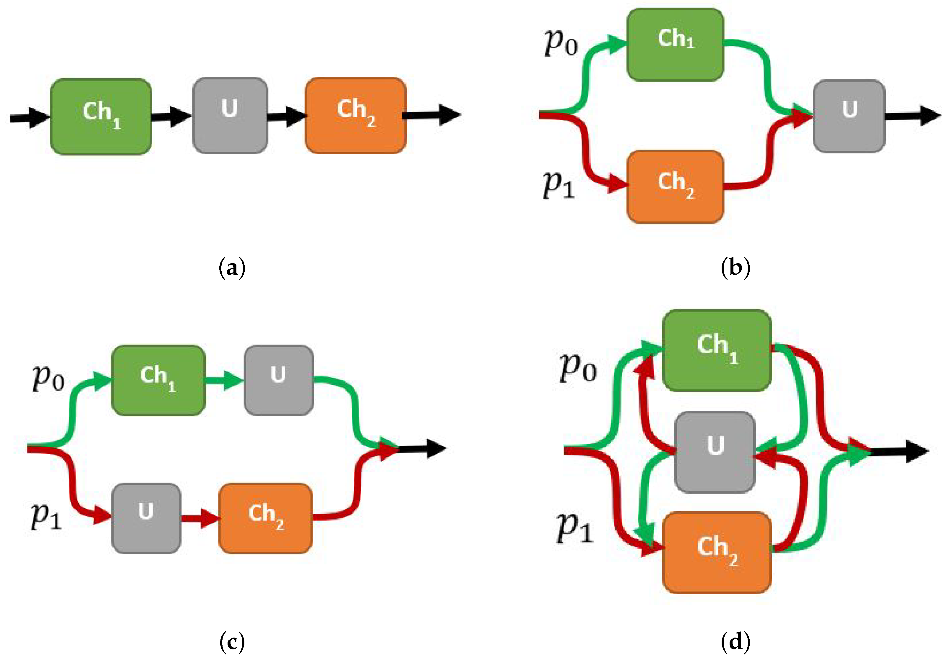
3.3. Some Concrete Architectures to Immerse Pauli Channels for the Improvement of QPE

Some cases of channel arrangements are shown in Figure 2. Those architectures have been proposed in the context of quantum circuits architecture, in particular for QPE to improve the parameter estimation [29], and additionally setting certain hierarchies in the estimation. Some types of configurations have been analysed by generalising or involving sequential and parallel channel processes and their superposition for a more effective channel discrimination [30]. By combining those types of connections, together with PS and/or ICO, they have been used to supersede channel noise or alternatively to improve QPE on certain specific channels as bit-flipping, depolarising, and amplitude damping [31]. In our current analysis, the use of some of these proposed architectures is considered for the entire Pauli channels family.

Figure 2a corresponds to a sequential arrangement (S + U), including an intermediate unitary control operation as that suggested by [28]: $U=e^{i\chi \hat{n}·\overrightarrow{\sigma }}=\cos \chi {\sigma }^0+i\sin \chi \hat{n}·\overrightarrow{\sigma }$, with $\hat{n}=(\sin \delta \cos ϵ,\sin \delta \sin ϵ,\cos \delta )$. Figure 2a and b correspond to superposition paths including the same previous unitary operation at the end (PS + U) or alternated (PSA + U) after and before as a function of the path. Finally, Figure 2d presents an indefinite causal order (ICO) arrangement (ICO + U) with the same intermediate unitary operation. Only the sequential arrangement does not require a control system (otherwise, it will remain separable through the process), which could be assumed to be prepared in the state $|{\psi }_C\rangle =\sqrt{p_0}|0_C\rangle +\sqrt{p_1}|1_C\rangle$. However, we should work on ${\rho }_C\otimes \rho$; our treatment has already integrated the control system in (6).

Thus, the output state of the sequential arrangement is simply expressed as the operation

$$\begin{array}{c}\hfill \mathsf{\Lambda }\left[\rho \right]=\sum _{i,j}{\alpha }_i{\alpha }_j{\sigma }^{j}U{\sigma }^i\rho {\sigma }^i{U}^{†}{\sigma }^j\end{array}$$

(18)

It still could be integrated into the scheme developed without depending on the control system. Then, each one of the four cases presented in Figure 2 could be respectively expressed as

$$\begin{array}{ccc}\hfill \mathrm{S}+U:& & C_{\alpha \beta ,\gamma }^{i_0{i}_1}=\sqrt{p_{\beta }{\alpha }_{i_0}{\alpha }_{i_1}}{\left[{\sigma }^{i_1}U{\sigma }^{i_0}\right]}_{\alpha \gamma }\hfill \end{array}$$

(19)

$$\begin{array}{ccc}\hfill \mathrm{PS}+U:& & C_{\alpha \beta ,\gamma }^{i_0{i}_1}=\frac{1}{2}\sqrt{p_{\beta }{\alpha }_{i_{\beta }}}{\left[U{\sigma }^{i_{\beta }}\right]}_{\alpha \gamma }\hfill \end{array}$$

(20)

$$\begin{array}{ccc}\hfill \mathrm{PSA}+U:& & C_{\alpha \beta ,\gamma }^{i_0{i}_1}=\frac{1}{2}\sqrt{p_{\beta }{\alpha }_{i_{\beta }}}{\left[{\sigma }^{\beta ·i_{\beta }}U{\sigma }^{\left(\beta \oplus 1\right)·i_{\beta }}\right]}_{\alpha \gamma }\hfill \end{array}$$

(21)

$$\begin{array}{ccc}\hfill \mathrm{ICO}+U:& & C_{\alpha \beta ,\gamma }^{i_0{i}_1}=\sqrt{p_{\beta }{\alpha }_{i_{\beta }}{\alpha }_{i_{\beta \oplus 1}}}{\left[{\sigma }^{i_{\beta \oplus 1}}U{\sigma }^{i_{\beta }}\right]}_{\alpha \gamma }\hfill \end{array}$$

(22)

where brackets ${\left[A\right]}_{\alpha \gamma }=A_{\alpha \gamma }$ refer to the entry $\alpha ,\gamma$ of A. Regarding U being unitary, it is easy to show that all cases fulfil the condition (7). Such expressions $C_{\alpha \beta ,\gamma }^{i_0{i}_1}$ work as structure constants from a transference function in (13) and () for each kind of channel. In those expressions, $p_{\beta }$ with $\beta =0,1$ are the probabilities for a control state defining the splitting through paths or causal orders, respectively. Notice that for the S + U case, the control is maintained just as a separable system to include it in the general procedure, and then its state is nonmeaningful in this case. Note that such expressions are quite valuable because expressions (6) and (8) allow for reaching $\mathsf{\Lambda }\left[{\rho }_{\mathrm{in}}\right]$ directly from ${\rho }_{\mathrm{in}}$.

The complexity should be clear now. Because of the large number of selectable parameters (those added to the ${\alpha }_i$ parameters being estimated), the optimisation problem moves into one of several variables: five (S + U) or even seven (for the remaining architectures). Then, an approach such as the Monte Carlo method becomes more practical because of the large number of selectable parameters.

4. Analysis of ${\mathcal{V}}_{\mathbf{h}}$ Bounds and Stochastic Affordability Provided by Several Architectures

To arrive at a comparison for the architectures being considered, we use the expression (4) to reach ${\mathcal{F}}_{ij}\left({\rho }_{\mathrm{out}}\right)$. This is possible through the value of ${\overrightarrow{n}}_{\mathrm{out}}$ coming from (12) by considering the initial state ${\overrightarrow{n}}_{\mathrm{in}}$ in ${\rho }_{\mathrm{in}}$ as function of $\theta ,\varphi$. The parameters $p_0$ for the control state (except for S + U) and $q_0$ for the final measurement basis on this system could be selected to improve the parameter estimation of ${\alpha }_i,i=1,2,3$. Additionally, the parameters $\delta ,ϵ,\chi$ are selectable for such a purpose. This implies five parameters for the S + U architecture (${\mathsf{\Pi }}^A=\{\theta ,\varphi ,\delta ,ϵ,\chi \}$) and seven for the remaining ones (${\mathsf{\Pi }}^B=\{\theta ,\varphi ,\delta ,ϵ,\chi ,q_0,p_0\}$).

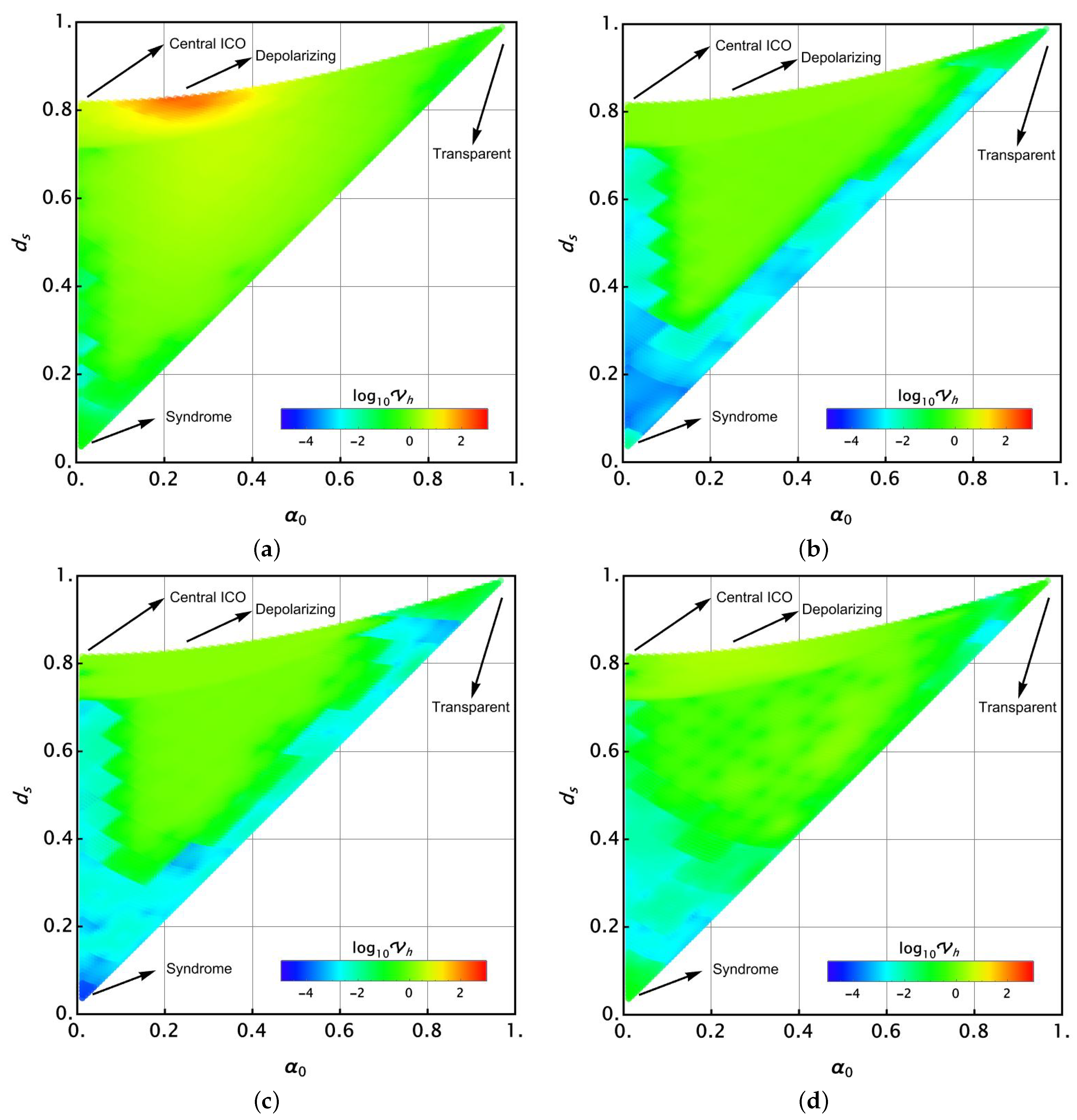
4.1. A Cross-Sectional Insight about QPE Using the Proposed Architectures

In an initial analysis, we will consider the simpler case for ${\alpha }_i=p,i=1,2,3,p\in [0,\frac{1}{3}]$ (the central line in the Pauli channel parametric space introduced in [23]). Figure 3a again reproduces that space as a reference, showing some emblematic Pauli channels: transparent channel (${\alpha }_i=0,i=1,2,3$) in the origin; depolarizing channel (${\alpha }_i=\frac{1}{4},i=1,\dots ,4$); central ICO channel (${\alpha }_i=\frac{1}{3},i=1,2,3$); and the three main syndromes in the tetrahedron corners (${\alpha }_i=1$ for just one $i=1,2,3$ at the time). Then, recursively using the Monte Carlo method on resizeable regions, we found the best set of five or seven parameters, minimising ${\mathcal{V}}_h$ for each architecture and point on the green line in the parametric space of Figure 3a.

Figure 3b shows the outcomes comprising the four architectures. For reasons of convenience, it has been represented as ${\log }_{10}{\mathcal{V}}_h$ instead of ${\mathcal{V}}_h$ directly. The black line shows the lower outcomes for the S + U case as a function of p. It exhibits certain expected outcomes: ${\mathcal{V}}_h$ drops to lower values for the transparent channel and ICO central channel but rises to infinity for the depolarising channel. In fact, it perfectly fits into the model ${\mathcal{V}}_h^{\mathrm{S}+\mathrm{U}}=\frac{0.0264}{{(p-0.25)}^2}$. Dashed blue and green lines respectively show the cases PS + U and PSA + U. Similarly, they show dramatically different outcomes for ${\mathcal{V}}_h$, providing much better expectations than the S + U case in almost all ranges for p. Still, the PSA + U case exhibits slightly better outcomes than the PS + U case, as can be seen in the lower inset for those two cases in a direct scale for ${\mathcal{V}}_h$. Interestingly, we found a discontinuity on the plot around $p=\frac{2}{30}\approx 0.067$. Discontinuities in QFI have been identified [32,33] generating this kind of outcome. Despite this, note the avoiding of the failed outcome near the depolarising channel as occurred for the S + U case. Finally, the ICO + U case still shows some improvements in some ranges. Near the transparent channel, this case does not reach better outcomes than the previous cases (this was already noticed by [9], still without the use of the added U transformations). One notable improvement occurs near p = 0.045, 0.09. In this last value, this case shows a discontinuity. The case for $p=0.045$ is not a discontinuity, but instead an effect of the ${\log }_{10}$-scale. Note the improved and the best values near $p\in [0.033,0.150]$ and also near the ICO central channel. Comparing the outcomes presented in [9], we conclude that the introduction of unitary operations in the architectures improves the outcomes in the bound for QPE for Pauli channels. In addition, here, we observe hierarchies as those observed and demonstrated by [28] for several similar architectures using the amplitude damping channel.

Table 1. Some representative values for ${\mathcal{V}}_h$ (on the central line as a function of p, and nearest to a pure syndrome) in each type of architecture.

Central Line $\left(\mathit{p}\right)$	${{\mathcal{V}}_{\mathit{h}}}^{\mathbf{S}}+\mathit{U}$	${{\mathcal{V}}_{\mathit{h}}}^{\mathbf{PS}}+\mathit{U}$	${{\mathcal{V}}_{\mathit{h}}}^{\mathbf{PSA}}+\mathit{U}$	${{\mathcal{V}}_{\mathit{h}}}^{\mathbf{ICO}}+\mathit{U}$
0.001	0.377	0.034	0.034	0.377
0.034	0.260	0.357	0.357	0.236
0.067	0.846	0.000	0.001	0.052
0.100	1.195	1.908	0.001	0.891
0.133	1.938	1.687	1.603	1.175
0.166	3.742	1.636	1.589	1.618
0.199	10.140	1.554	1.624	2.142
0.232	81.385	1.498	1.498	2.855
0.265	117.189	1.564	1.564	3.186
0.298	11.446	1.498	1.498	2.239
0.331	4.024	1.294	1.294	1.018
Syndrome $({\alpha }_i=1)$	0.245865	0.037687	0.000023	0.243448

reports some representative values for each architecture and several values of p to set the dimensions represented in Figure 3. Prescriptions for other selectable parameters $\theta ,\varphi ,\delta ,ϵ,\chi ,q_0,p_0$ in each architecture case become nonmeaningful to be reported because, in fact, there are multiple solutions for the optimisation, as it will be analysed below. Our procedure of search is stochastic, but converging to the best solution with the minimal ${\mathcal{V}}_h$. Nevertheless, in most cases, several solutions were found. These values show important improvements with respect to those obtained using just single sequential or ICO arrangements in [9] because of the inclusion of U operations. A complete analysis of all the Pauli channels is difficult in terms of computer processing times. However, the channels on the central line are notable, and other cases of the channels with representative syndromes are also of interest. In the next subsection, we develop an analysis around them to compare the four architectures.

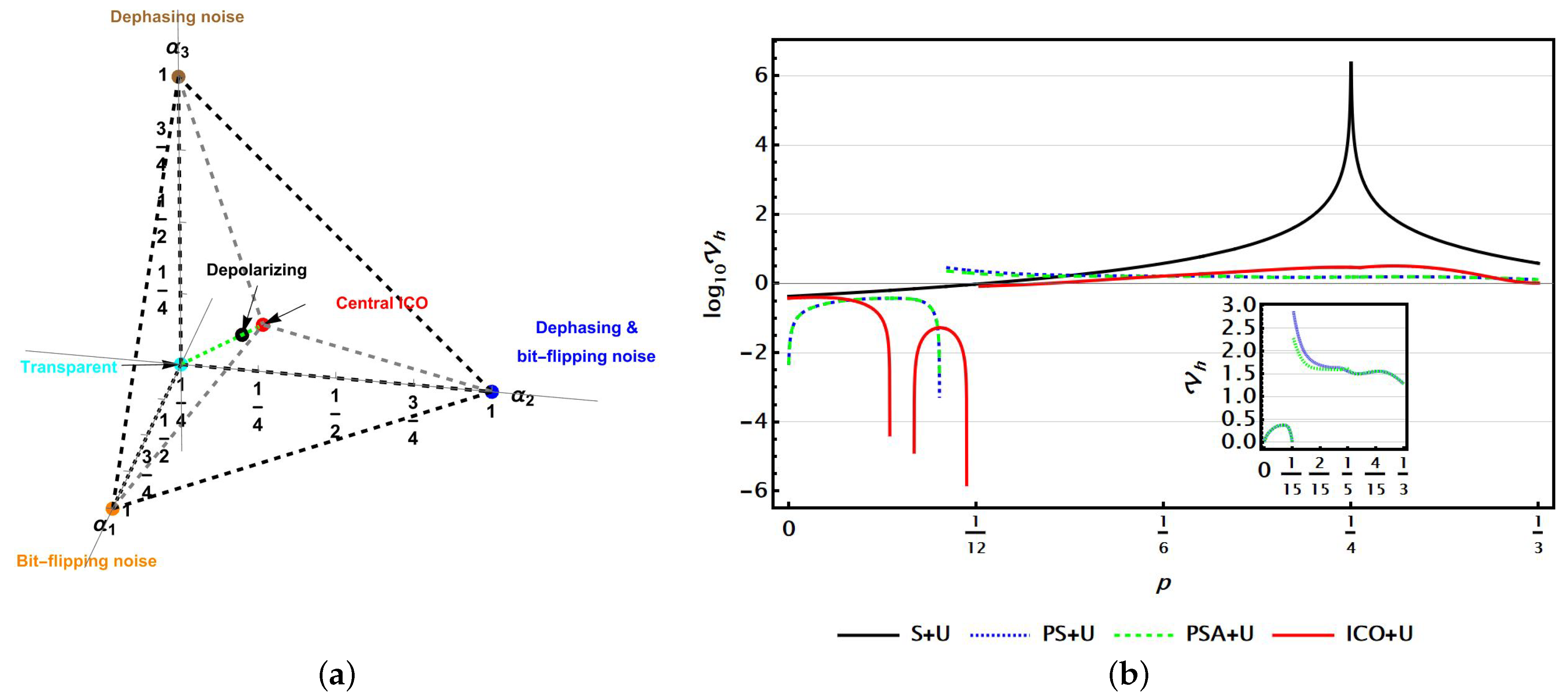
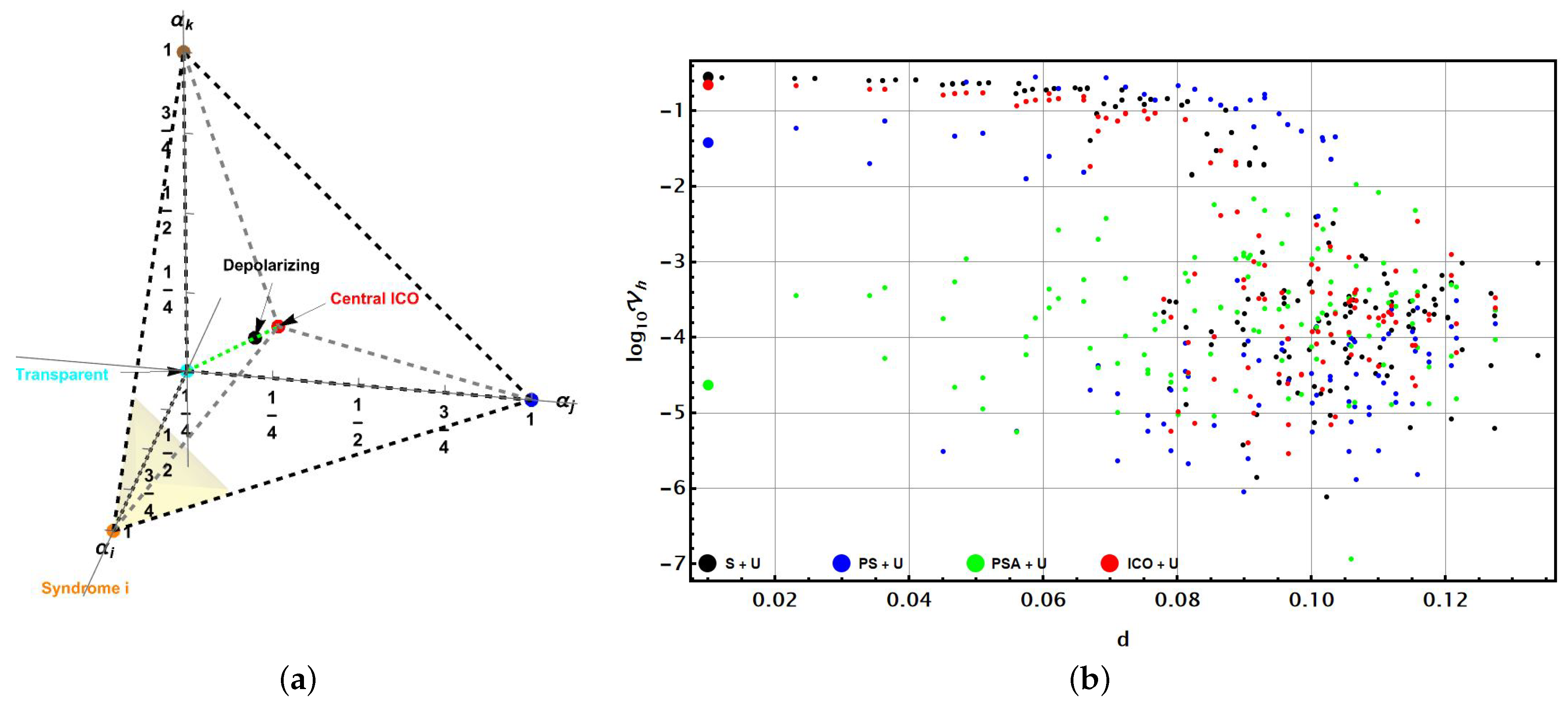
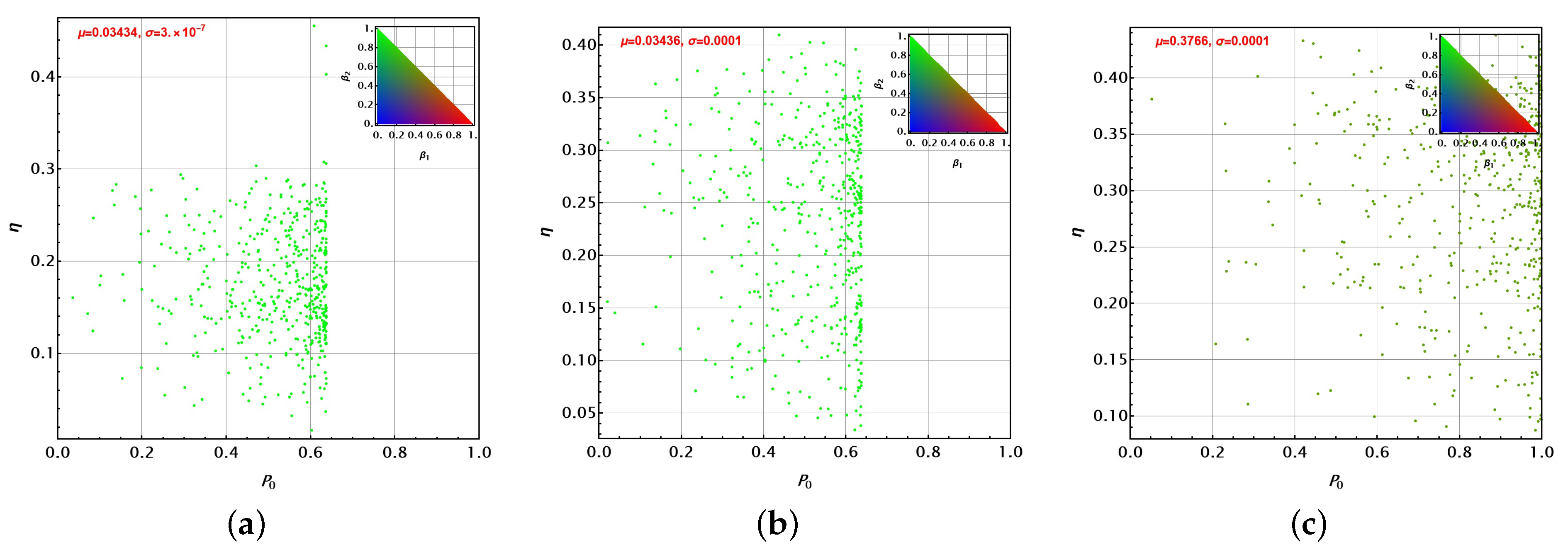
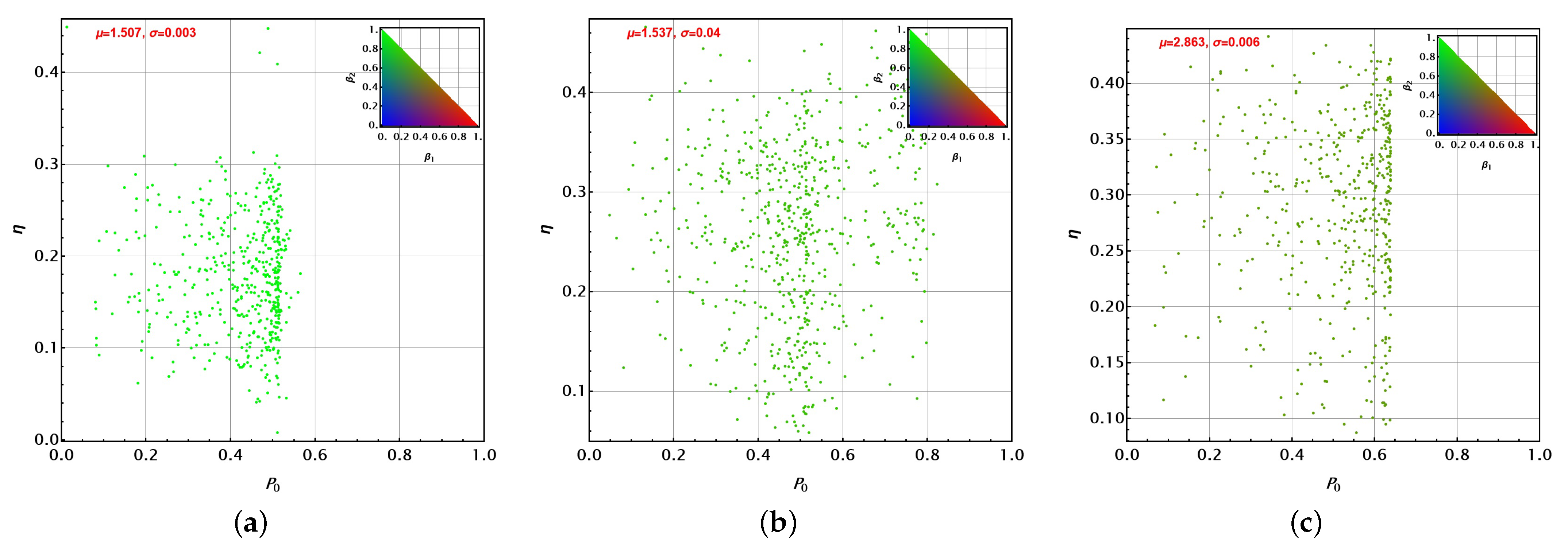
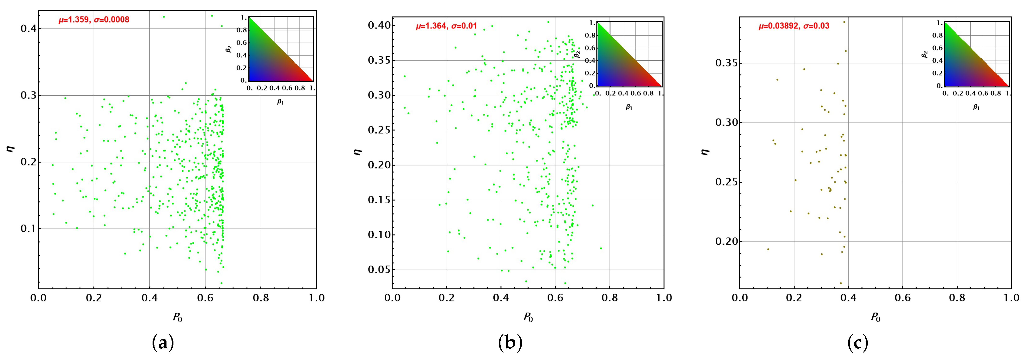
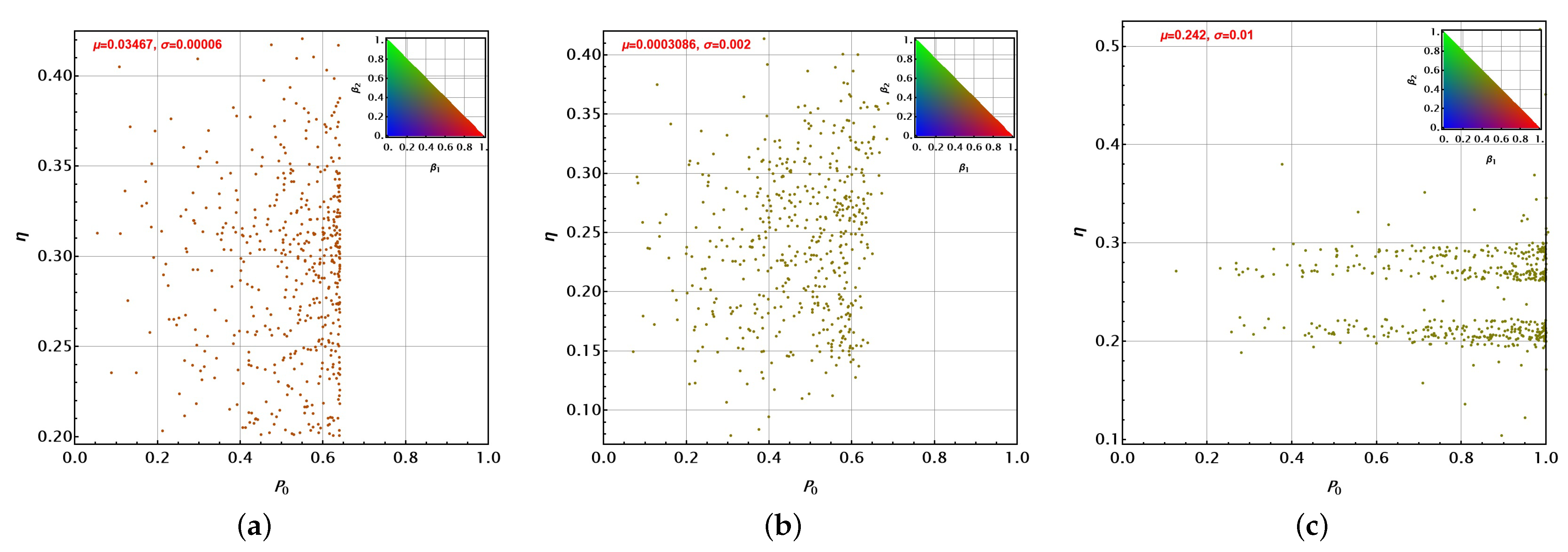
4.2. Analysis of QPE Using the Proposed Architectures around Typical Syndromes for Pauli Channels

Error syndromes for Pauli channels correspond to the cases ${\alpha }_i=1$ for each $i=1,\dots ,3$ at the time: bit flipping noise ($i=1$), dephasing noise ($i=3$), and a combination of both ($i=2$). Note that all three cases should be analysed because QFI is invariant upon a cyclic permutation of Pauli matrices (it is easy to notice because by a proper basis change, ${\sigma }^1,{\sigma }^2,{\sigma }^3$ become cyclically exchanged). Thus, we will analyse the case with $0.9\le {\alpha }_i\le 1$ near the syndrome i in agreement with the last description. It is a corner including the Pauli channels nearest to one of those syndromes. By considering a uniform sample of channels in that region for each architecture, we obtained an insight into the ${\mathcal{V}}_h$ behaviour.

Figure 4 shows the outcomes. Each dot represents the outcome of a channel and architecture. Outcomes are presented as a function of ${\mathcal{V}}_h$ and the distance d to the channel exhibiting the pure syndrome just in the corner $({\alpha }_i,{\alpha }_j,{\alpha }_k)$, with ${\alpha }_i=1$ and $i,j,k$ a cyclic permutation of $1,2,3$. The dot colour represents the architecture used in agreement with those colours used in Figure 3. Due to the different scales of the outcomes, a ${\log }_{10}$-scale has been used again. They were generated by sampling the shadowed wedge region shown in Figure 4a. Sampling was performed as Cartesian uniform in the region. The biggest points on the left of Figure 4b correspond to the closest to the syndrome channel considered in the corner.

In this case, the S + U (black points) and ICO + U (red points) cases give similar outcomes for ${\mathcal{V}}_h$. No deeper advantage is noticed by the use of ICO in the architecture. It was already noticed in [9] for syndrome channels. In fact, the biggest black and red points meet, but they were artificially displaced a little just to be distinguished on the plot. Instead, the PS + U (blue points) and PSA + U (green points) cases exhibit much better outcomes for QPE. However, the PSA + U architecture still improves the outcomes for the parameter estimation near the syndrome channel, thus giving ${\mathcal{V}}_h$ values below ${10}^{-4}$. We note that the PS + U case shows a two-fold approach near the syndrome channel, but finally converging on the biggest blue point on the left. All values for ${\mathcal{V}}_h$ nearest to the syndrome channel (biggest points in Figure 4b) have been reported in the last row of Table 1.

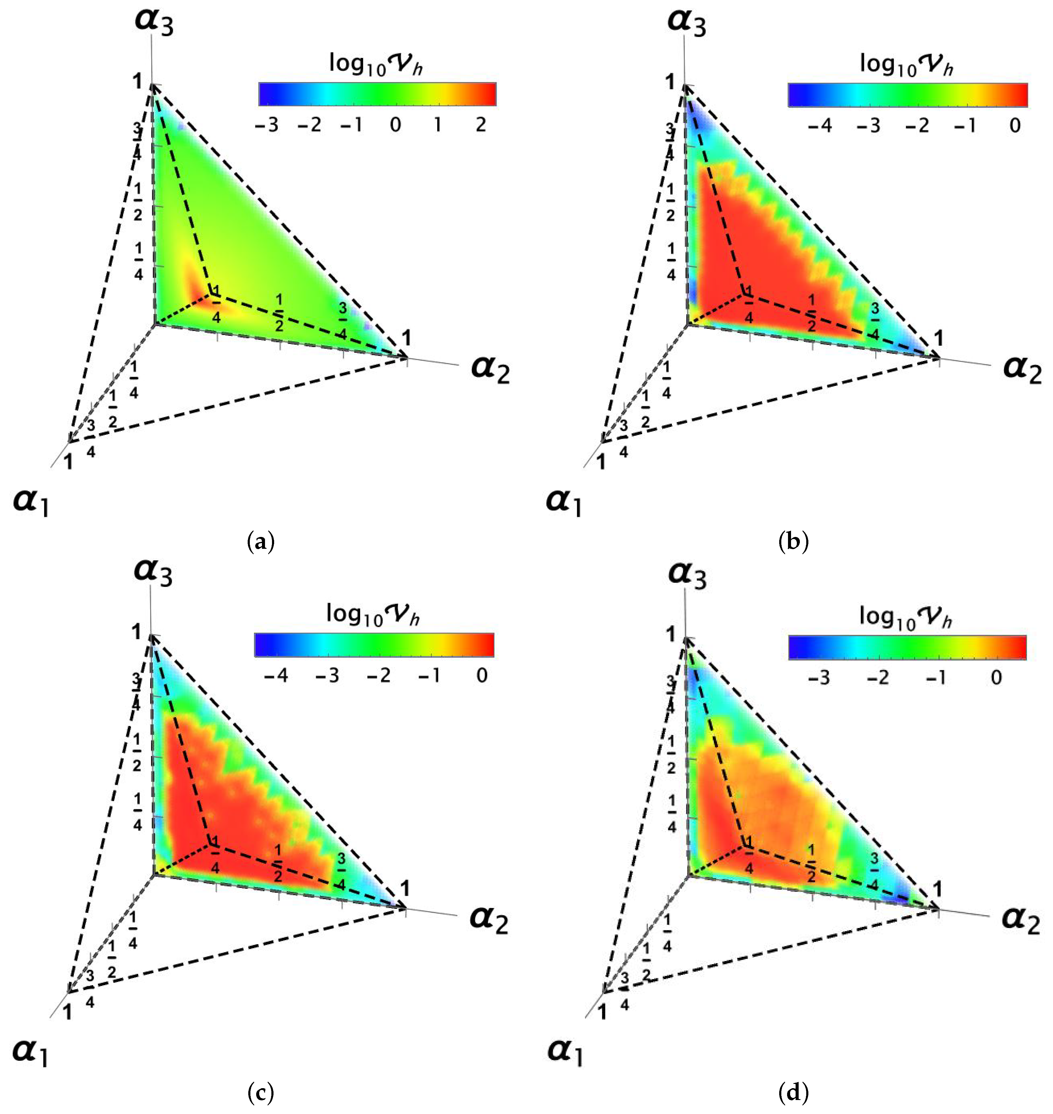
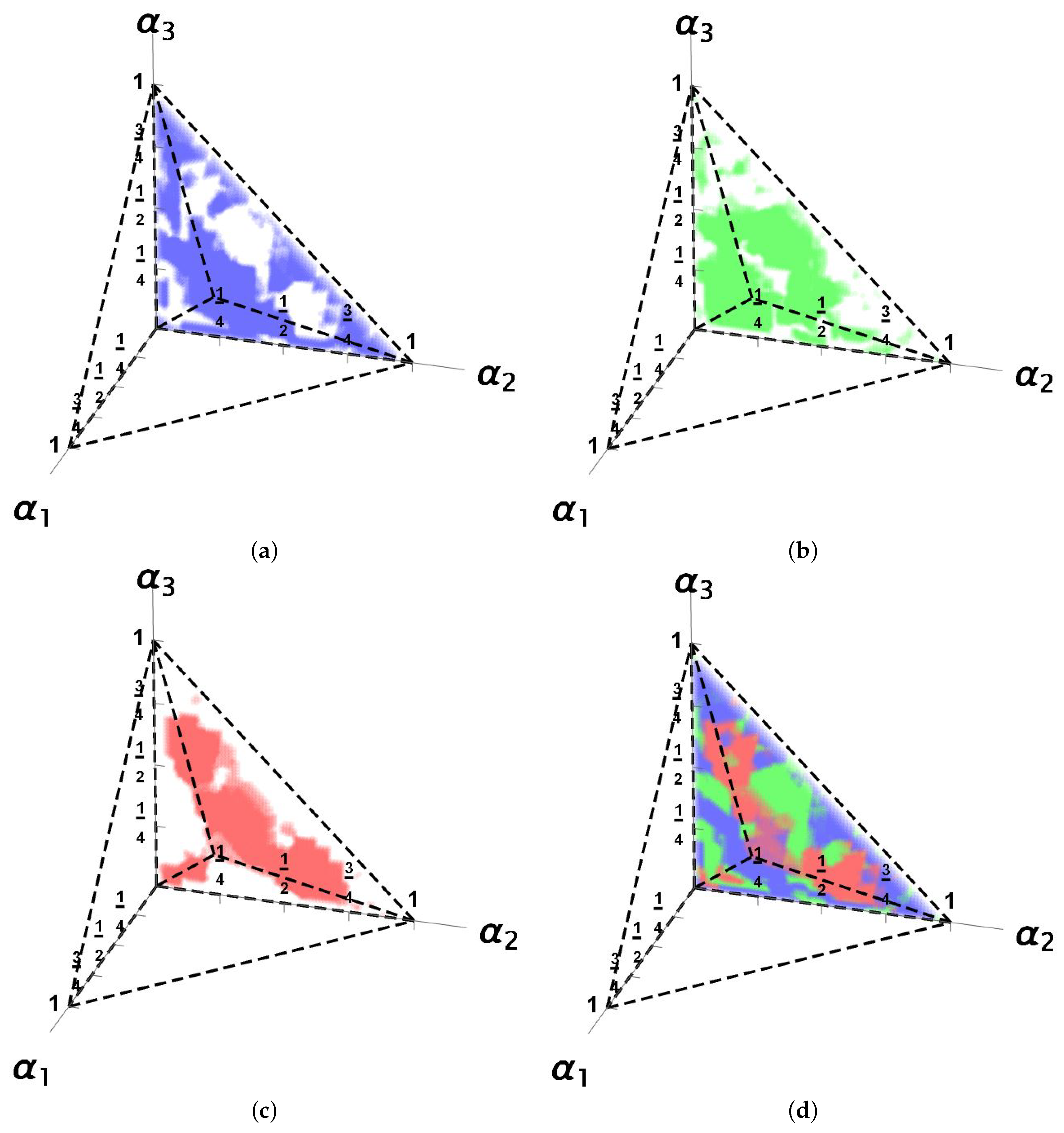
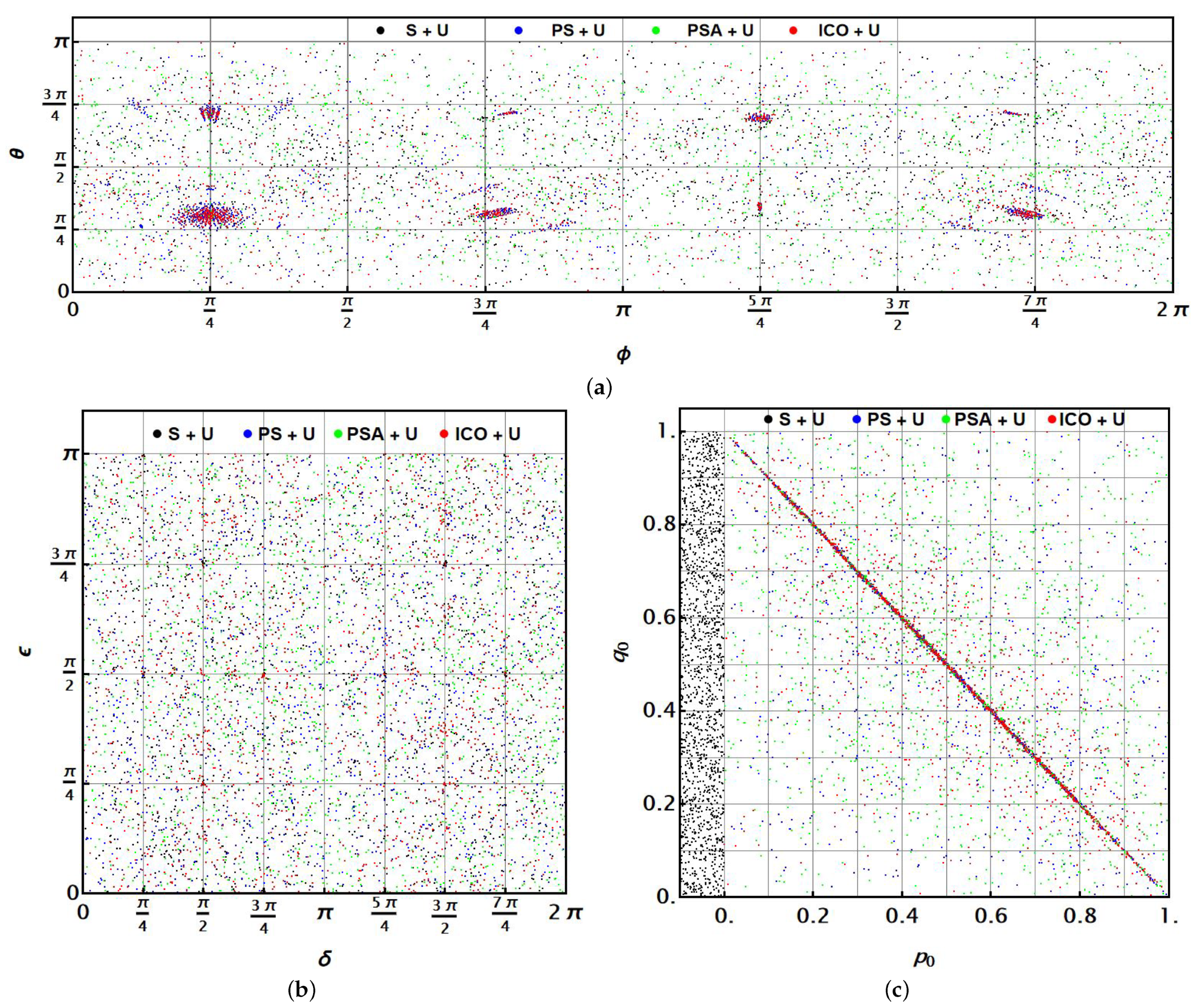
General Overview of QPE on the Entire Pauli Channels Parametric Space

Figure 5 presents for the multiparametric case an analysis of ${\mathcal{V}}_h$ for each architecture in the overall parametric space of Pauli channels. Each panel exhibits the outcome for each given architecture.

For this analysis, a couple of 12-core computers with processors of 3.4–3.5 GHz and the evaluation for an optimised value of ${\mathcal{V}}_h$ following the recursive Monte Carlo method on resizeable regions of convergence have been used. This is a computer task lasting between 2 and 5 min (depending on the architecture) for every single point on the parametric space of the Pauli channel parameters. In this work, a sweep on the parametric space has been developed by using 3000 evaluation points for each architecture to obtain a representation of the optimised ${\mathcal{V}}_h$ there. To improve the detailed evaluation, the process has used an interpolation function over those points based on the nearest neighbours effectively calculated in the optimisation process. This interpolation has considered the inverse quadratic distance to the interpolation point as weight. Thus, it provides a more detailed three-dimensional map of that bound on the entire parametric space.

In these general views on optimised QPE for the overall Pauli channels, the previous outcomes become consistent. Figure 5a shows the sequential case with the values for ${\mathcal{V}}_h$ in colour, in agreement with the colour bar at the top. In this case, ${\mathcal{V}}_h$ is mostly near by units, but much nearer to the depolarising channel (again, outcomes are presented using a ${\log }_{10}$ scale in a proper range for each architecture to better notice the gradient). Only the syndromes exhibit lower values, while in the remaining regions, ${\mathcal{V}}_h$ is around the units. Figure 5b,c show the superposition path cases being considered, where PSA + U has improved values but, in general, the best ranges among the four architectures. Note particularly that the best outcomes for PSA + U in the channel syndromes are almost unnoticed because, in their proximity, PS + U still provides better outcomes (see, as a comparison, in Figure 4b, the group of blue dots with lower ${\mathcal{V}}_h$ values than those in green). Note in both cases that the discontinuities are near the transparent channel in the origin. For the ICO + U case, better outcomes are obtained in the central region of the tetrahedron, together with comparable outcomes near the channel syndromes, as was already noticed in Figure 4. In general, the poorest outcomes in the centre of the parametric space were already observed for those configurations without the support of unitary operations [9]. Despite this, these outcomes now show that the inclusion of complementary unitary operations becomes valuable in the improvement of ${\mathcal{V}}_h$ and QPE.

An alternative two-dimensional view of the last outcomes has been constructed by representing the values of ${\log }_{10}{\mathcal{V}}_h$ as a function of ${\alpha }_0$ and the minimum distance to the closer syndrome, $d_s$ (they are suggested by the three-dimensional plots in Figure 5). In such a representation, dots become superposed. Figure 6 shows those representations for (a) S + U, (b) PS + U, (c) PSA + U, and (d) ICO + U. In this case, the same colour scale has been used to ease the comparison between the architectures. There, ${\log }_{10}{\mathcal{V}}_h$ is reported. In addition, the main emblematic channels have been signalled: transparent, syndrome, depolarising, and central ICO channels. In this representation, the three borders of the plotted region correspond to (a) the central line ${\alpha }_1={\alpha }_2={\alpha }_3$ analysed in Section 4.1 (upper frontier), (b) the line along each ${\alpha }_i$ axis ${\alpha }_j={\alpha }_k=0$ (rightmost frontier), and (c) the line connecting the central ICO channel with the syndrome ${\alpha }_i=1$, meaning ${\alpha }_j={\alpha }_k$ (leftmost frontier). This representation clearly exhibits the goodness of each architecture by region. The observations fit with the previous discussion of Figure 5. Note particularly the advantage of PSA + U very near to the syndrome and also the limited advantage of using an architecture involving ICO.

A final analysis to set a hierarchy among the architectures could be obtained by comparing the bounds found for each channel. Thus, for the multiparametric case, Figure 7 shows the regions where each architecture provides the lowest bound. The S + U case was omitted because, for every channel, it always provides the worst bounds. All other architectures have channel regions with the best bound among the three cases: Figure 7, (a) PS + U (blue); (b) PSA + U (green); and (c) ICO + U (red). Again, just one-third of the entire parameter space is illustrated for clarity. The grainy structure of these regions is notable (note particularly the entire picture in Figure 7d, already noticed in Figure 5 and Figure 6, instead of well-defined three-dimensional regions as those cases reported in [9], not considering the support of unitary controls). In these architectures, control unitary operations finally efficiently drive the manipulation process to address an improved QPE.

The set of parameters ${\mathsf{\Pi }}^A=\{\theta ,\varphi ,\delta ,ϵ,\chi \}$ for S + U and the set ${\mathsf{\Pi }}^B=\{\theta ,\varphi ,\delta ,ϵ,\chi ,q_0,p_0\}$ for PSA + U, PS + U, and ICO + U admit several optimal values in the analysis because the solutions are nonunique. It will be interesting to analyse them for the sake of some important possible correlations among those selectable parameters for the optimal solutions.

Figure 8 shows some of those outcomes corresponding to all the solutions presented in Figure 5. They have been paired to reveal some possible correlations among those selectable parameters. Figure 8a compares, for each architecture identified in colour as the upper legends remark, the solutions for the pair $\theta ,\varphi$. Although many of those pairs become uniformly dispersed, certain accumulation points exist for PS + U (blue), PSA + U (green), and ICO + U (red). Be aware of some shadowing among the point groups for each architecture meeting in the same region. However, this behaviour is not observed for the S + U (black) case. Those accumulation points are real considering that the sampling was performed using the Haar measure. Similar accumulation points were also noticed in previous analyses for probe states not using the support of unitary operations as in the current proposals [9]. In any case, comparing those outcomes with the current ones, we observe the valuable introduction of those complementary operations in the lowering of the CRB for Pauli channels.

In another view, the pairs $\delta ,ϵ$ are presented in Figure 5b. It is clear that in any case there are no evident correlations between this pair of parameters, which now are completely and uniformly distributed. This indicates that unitary operations (rotations on the Bloch ball) do have not a privileged direction relating each parameter with another. Finally, Figure 5c shows the relation between $q_0$ and $p_0$ for PS + U (blue), PSA + U (green), and ICO + U (red) cases. Notably, many optimised solutions exhibit the relation $q_0\approx 1-p_0$, as it becomes evident from the plot.

Because for S + U, the form (19) has been maintained, including a control remaining separable from the system, to then follow the same computational procedure as in the other architectures, certain values for $q_0$ were obtained (the initial state for the control was fixed in this particular case as $p_0=p_1=\frac{1}{2}$), but in this case, they are expected to be random. Thus, in a different representation, for such an S + U case (black), the leftmost fringe is included in the same plot for comparison to verify this expected behaviour. This presents the solutions for $q_0$ in the S + U case, using only the vertical axis. There, each solution was randomly displaced through the fringe widely, using the nonmeaningful horizontal direction, to exhibit the corresponding and expected uniform distribution for $q_0$ values.

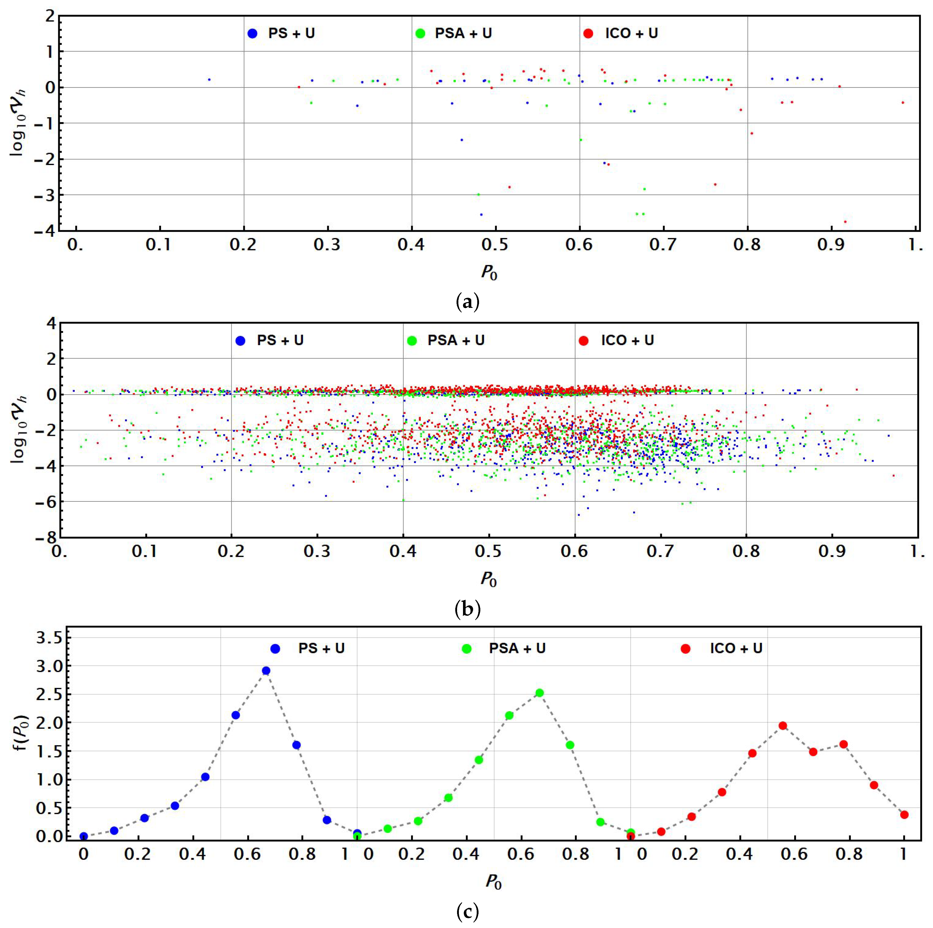
4.3. Some Final Considerations Related to the Success Probability $P_0$

Appendix B reports the expressions for $P_0$ in each architecture. Unfortunately, the expressions for ${\overrightarrow{n}}_{\mathrm{out}}$ are very complex when they are expressed in terms of the parameter sets ${\mathsf{\Pi }}^A$ and ${\mathsf{\Pi }}^B$ to be reported there. In this subsection, an analysis of the $P_0$ values is performed. Figure 9 synthetically reports the analysis. In this analysis, clearly, for the reasons previously discussed, the case S + U has not been considered.

Considering that the optimisation problem exhibits multiple solutions in spite of the number of selectable parameters, it is not expected that $P_0$ consistently exhibits the largest possible values. Thus, the outcomes for the previous analysis have simply been used to analyse the behaviour of the success probability $P_0$. Because the concrete values for the parameters p or ${\alpha }_1,{\alpha }_2,{\alpha }_3$ will hardly show a certain correlation with $P_0$, the analysis for this value is correlated with the value of ${\mathcal{V}}_h$ (or ${\log }_{10}{\mathcal{V}}_h$ in the plots). Thus, for the reduced number of solutions obtained in the single parameter case characterized by p, Figure 9a shows the corresponding correlations between $P_0$ and ${\log }_{10}{\mathcal{V}}_h$. Again, each architecture is coloured as before. Each dot represents one solution through the central lines for a given architecture. All cases PS + U, PSA + U, and ICO + U exhibited $P_0$ values regularly over $P_0>0.5$ in most cases.

With the multiparametric case (see Figure 9b), because of the large number of solutions analysed, previous behaviours become confirmed. Those architectures show values barely centred on $P_0\approx$ 0.5–0.6, thus providing certain effectivity. In particular, the case PSA + U appeared providing the highest values for $P_0$. Considering that the optimal solutions in the entire space of parameters ${\mathsf{\Pi }}^B$ were obtained from a uniform distribution of them, the last observations can be verified in Figure 9c. There, numerical probabilistic distributions $f\left(P_0\right),P_0\in [0,1]$ for $P_0$ values in the Monte Carlo procedure have been obtained for each architecture through the three panels. Interestingly, the ICO + U case shows a two-peaked distribution (a double-check was made to verify this fact). Otherwise, the PS + U case shows a narrower distribution than the PSA + U one, which has little advantage in the mean. In any case, all distributions are right-skewed. These outcomes suggest that among the multiple solutions for the optimisation problem for ${\mathcal{V}}_h)$, the values for $P_0$ (without additional optimisation) have on average reasonable values favouring the stochastic process on the control system to perform the channel parameters estimation. Still, an improved search could reach both optimisations, on ${\mathcal{V}}_h$ and $P_0$.

5. Discussion of Outcomes and Improving the Stochastic Affordability

In spite of the previous outcomes and comparing them with those presented in [9], it becomes clear that the use of control unitary operations provides notable outcomes for QPE for single Pauli channels when they are combined under architectures using sequential, superposition paths, or even ICO Pauli channel arrangements. Because of the number of parameters, even with our numerical approach used in the optimisation process, the existence of multiple solutions became evident. Because the procedure is stochastic, its affordability is linked to the possible $P_0$ values of success. These solutions should require parallel optimisation for such variables. Clearly, we avoid the S + U case because of the absence of control.

In the current section, the previous outcomes in QPE are analysed for some emblematic channels under the architectures presented, but this time, the analysis emphasises the role that $P_0$ plays in the entire process. Then, a different analysis will be performed. Because the previous optimal outcomes are multiple, our previous analysis was free, in some sense, of the specific selectable parameters’ values (more than the optimisation for the lower bound of ${\mathcal{V}}_h$). Thus, in the current analysis, sets of identical optimal solutions providing the same lowest bound for each case analysed will be gathered to analyse their feasibility as given by $P_0$. In such a case, each element of the set of optimal solutions for the QPE problem will provide a different value for $P_0$, some of them becoming more convenient in the process as a consequence. For such a purpose, only the transparent, depolarising, central ICO, and syndrome (bit-flipping) channels will be considered as exemplary channels. For each channel, a wide set of optimal solutions in terms of ${\mathcal{V}}_h$ will be newly obtained. For instance, Figure 10 presents the outcomes for the transparent channel in terms of several analysis parameters defined as follows.

Through the analysis, we will deal with several parameters. In each case, we obtain a set of 500 optimised solutions for each channel estimation and architecture used, each one gathering the same optimal bound but delivering different values for $P_0$. We tracked the selectable parameters of optimisation to determine $P_0$ through the formulas reported in Appendix B. Because the procedure to obtain those solutions is stochastic, tiny numerical variations on ${\mathcal{V}}_h$ could be obtained. Thus, to assess such a fact, each set was characterized by its mean $\mu$ and standard deviation $\sigma$ (expected to be small), which are reported on the left top of each panel plot. In addition, for each set, the geometric average for each one of the seven selectable parameters ${\overline{\mathsf{\Pi }}}^B=\{\overline{\theta },\overline{\varphi },\overline{\delta },\overline{ϵ},\overline{\chi },{\overline{q}}_0,{\overline{p}}_0\}$ was calculated. Then the parameter:

$$\begin{array}{c}\hfill \eta =\frac{1}{{\eta }_{\max }}\left|\right|{\mathsf{\Pi }}^A-{\overline{\mathsf{\Pi }}}^A\left|\right|\end{array}$$

(23)

was calculated by each solution (dot). There, ${\eta }_{\max }={\max }_{{\mathsf{\Pi }}^A}\left\{\right||{\mathsf{\Pi }}^A-{\overline{\mathsf{\Pi }}}^A\left|\right|\}=\sqrt{2+14{\pi }^2}$ is the maximum distance in the seven parameter dimensions. Such a parameter provides information about how far each solution is from the average in the set. Additionally, we have grouped the parameters into three groups: $g_1=\{\theta ,\varphi \},g_2=\{\alpha ,ϵ,\chi \},g_3=\{q_0,p_0\}$. Then, by obtaining the composed variance of each set $v_i=\frac{1}{{\mathcal{C}}_i}{\sum }_{j\in g_i}\mathrm{var}\left(\left\{{\pi }_j\right\}\right)$, ${\mathcal{C}}_i$ being the cardinality of each subset $g_i$. Then, the three parameters ${\beta }_i$ are defined as

$$\begin{array}{c}\hfill {\beta }_i=\frac{v_i}{{\sum }_{i=1}^3{v}_i}\end{array}$$

(24)

Clearly, ${\beta }_1+{\beta }_2+{\beta }_3=1$. Each one of these parameters independently reflects the variation of each set of parameters with respect to their averages. Thus, because of the normalisation introduced, the larger will denote the main source of variation in each set of solutions. Thus, in the following Figure 10, Figure 11, Figure 12 and Figure 13, the dot colour for each set represents a red–green–blue (RGB) mixture reflecting that balance: the probe state (red), the unitary control (green), or the control state definition and its optimal measurement (blue). The colour is then settled by the colour scale in the triangular chart at the top right as a function of ${\beta }_1$ and ${\beta }_2$ (${\beta }_3=1-{\beta }_1-{\beta }_2$). Thus, Figure 10 presents several facts. First, parameters $P_0$ appear upper-bounded approximately by $0.65$ for the PS + U and PSA + U cases. This is not observed for the ICO + U case. Dispersion around the average is comparable for the three cases (values of $\eta$). In addition, the main source of variation is due to the unitary control U parameters for PS + U and PSA + U (${\beta }_2\approx 1$). For the ICO + U case, the variation due to the probe state becomes a little more important than in the previous cases. Almost no variation is due to the control state. The parameters $\mu$ and $\sigma$ show only tiny variations obtained by our optimisation procedure to reach the optimised solutions.

For the depolarising channel in Figure 11, the consistency of the sets (given by $\mu$ and $\sigma$) is also high. Note that in general, for the overall cases analysed, the $\mu$ values are consistent with our previous analysis outcomes in Section 4.1 and Section 4.2. In this case, the three architectures show upper-bounded values for $P_0$, being better for the PSA + U case and the worst for the PS + U one. The selectable parameters’ source of variation is barely similar to those of the transparent channel. With similar structural characteristics, Figure 12 shows the corresponding outcomes for the central ICO channel, noting in all cases upper bounds for $P_0$, the worst for the ICO + U case, and the best for the PSA + U case. This last case exhibits a little higher variation due to the probe state. Note how the set of solutions for the ICO + U case overlaps recurrently. As for the depolarising channel, and as for the central ICO one, the dispersion provided by $\eta$ becomes comparable. In this case, the variation for the ICO + U case is more strongly dependent on the probe state.

Finally, Figure 13 presents the corresponding outcomes for the pure syndrome case (currently, the bit-flipping channel was analysed). In this particular case, we note that the probe state introduces a more important source of variation than in all previous cases, thus changing the dot colours. Again, only for the ICO + U architecture, the $P_0$ values become not bounded. Interestingly, different from all the previous cases, the ICO + U architecture used for the pure syndrome estimation exhibits a two-peak narrow distribution for $\eta$, instead of the single observed previously. Again, the values reported for $\mu$ are consistent with our previous discussion for the syndromes case.

6. Conclusions

In the previous sections, an analysis to address the QPE problem on Pauli channels was developed by combining each channel under analysis together with other identical channels and additional local control operations, always within composed arrangements or architectures. These architectures include additional free parameters not under analysis, but instead selected to improve the QPE outcome. The architectures considered include parallel paths and indefinite causal structures, while local operations U are located inside the arrangements.

In the analysis, an analytical approach was presented to construct the Kraus operators of those combinations as expressed through Formulas (19)–(22). For Pauli channels (and channels for local $n-$level systems), the expression (4) for QFI exploits the Bloch representation of those systems to obtain an affordable expression for the analysis. Thus, the channel effect is reduced to analyse the change on the Bloch state vector ${\overrightarrow{n}}_{\mathrm{in}}$ into ${\overrightarrow{n}}_{\mathrm{out}}$ coming out from it. Nevertheless, although expressions for the QFI matrix ${\mathcal{F}}_{ab}\left({\rho }_{\mathrm{out}}\right)$ are achievable, due to their complexity, they should still be analysed to reach ${\mathcal{V}}_h$ (inverting and tracing) due to the presence of a large number of selectable parameters ${\mathsf{\Pi }}^A$ or ${\mathsf{\Pi }}^B$ (in addition to the estimation parameters ${\alpha }_i$). The first parameters should be numerically analysed to optimise the QPE by minimising ${\mathcal{V}}_h$, which represents a complex analytical problem in general.

By proceeding numerically, we swept the selectable parameters under a numerical stochastic approach to reach the optimal values of ${\mathsf{\Pi }}^A$ or ${\mathsf{\Pi }}^B$ for each possible Pauli channel. This outcome is notable because, under the same analysis, the entire Pauli channels family has been analysed, instead of only particular channel cases. Upon the consideration of a single-parameter approach $p={\alpha }_i\in [0,\frac{1}{3}],i=1,2,3$, a first insight for the four architectures considered (S + U, PS + U, PSA + U, and ICO + U) was reached. In that region, the PS + U and PSA + U arrangements exhibited a certain superiority, minimising ${\mathcal{V}}_h$ for most of the p values. Despite this, the ICO + U scheme shows regions of superiority (see Figure 3).

For the multiparametric estimation, the analysis also already denotes the advantages of PS + U and PSA + U in the neighbourhood of pure syndrome channels, more highly remarked for the latter scheme over several magnitude orders for ${\mathcal{V}}_h$. Then, for the global analysis, the advantage or hierarchy among schemes shows a patched structure (see Figure 5, Figure 6 and Figure 7), always superseding the sequential scheme. In general, by comparing those outcomes in [9] with the current ones, including the support of the local control operations U, it is clear that in general, several magnitude orders of improvement are reached. For certain channels, the inclusion of more than two identical channels, as in [9], could still improve the outcomes presented if control operations U are already considered.

In the architectures regarded, due to a large number of selectable parameters, it is found that multiple optimal solutions for the minimum of ${\mathcal{V}}_h$ exist. In addition, because a stochastic solution is used, which is based on the control measurement to dispose of it (which clearly simplifies the analysis), it imposes limitations under a more general approach. In any case, those selectable parameters only exhibit partial correlations for the selection of the probe state (in particular, for architectures other than S + U), but more remarkably for the relation between the control state used and their optimal pretended outcome measurement. On the other hand, the selection of U as the key element in this analysis appears to attend more to each channel’s own characteristics instead of another underlying pattern.

The success of the stochastic procedure (introduced by the control measurement), as measured by $P_0$, becomes relatively affordable for a unit probe (considering each experiment can be repeated N times), exhibiting values around $0.6$ upon a nonplanned selection. Nevertheless, the number of parameters also allows improved solutions to be reached for $P_0$ (see Figure 9c) in addition to ${\mathcal{V}}_h$. Still, such selection becomes limited in several cases not reaching perfect values (see Figure 10, Figure 11, Figure 12 and Figure 13). The variability of those solutions becomes remarkably imposed by the selection of U than from the probe state selection. This fact fits with the outcome presented by Figure 8b.

As a final remark for the analysis presented, note that the existence of architectures with improved lower bounds for the QPE variances only states the possibility to reach more accurate estimations for the channels’ parameters. Still, on the other hand, novel techniques to set proper estimators experimentally reaching the estimation problem are in order [34]. In addition, upon an unknown channel, it could be difficult to impose the prescriptions found here because they precisely depend on the channel’s nature. Instead, a multistep procedure in the estimation should be followed to first reach a certain insight into the channel as the quantum benchmarking approach [17] or other more direct approaches [35], and then more complex and elaborate approaches in terms of the current architectures should be pursued.

References

1. Lehmann, E.L.; Casella, G. Theory of Point Estimation; Springer: New York, NY, USA, 1986. [Google Scholar]
2. Fujiwara, A. Quantum channel identification problem. Phys. Rev. A 2001, 63, 042304. [Google Scholar] [CrossRef]
3. Fisher, R.A. On the Mathematical Foundations of Theoretical Statistics. Philos. Trans. R. Soc. Lond. Ser. A 1922, 222, 594–604. [Google Scholar]
4. Helstrom, C. Quantum Detection and Estimation Theory; Academic Press: New York, NY, USA, 1976. [Google Scholar]
5. Rao, C.R. Information and accuracy attainable in the estimation of statistical parameters. Bull. Calcutta Math. Soc. 1945, 37, 81–91. [Google Scholar]
6. Frieden, B.R.; Gatenby, R.A. Principle of maximum Fisher information from Hardy’s axioms applied to statistical systems. Phys. Rev. E 2013, 88, 042144. [Google Scholar] [CrossRef] [PubMed]
7. Chiribella, G.; D’Ariano, G.M.; Perinotti, P. Quantum circuit architecture. Phys. Rev. Lett. 2008, 101, 060401. [Google Scholar] [CrossRef]
8. Ebler, D.; Salek, S.; Chiribella, G. Enhanced Communication with the Assistance of Indefinite Causal Order. Phys. Rev. Lett. 2017, 120, 120502. [Google Scholar] [CrossRef] [PubMed]
9. Delgado, F. Symmetries of Quantum Fisher Information as Parameter Estimator for Pauli Channels under Indefinite Causal Order. Symmetry 2022, 14, 1813. [Google Scholar] [CrossRef]
10. Frey, M.; Collins, D. Quantum Fisher information and the qudit depolarization channel. Proc. SPIE Quantum Inf. Comput. VII 2009, 7342, 73420N. [Google Scholar]
11. Procopio, L.M.; Delgado, F.; Enríquez, M.; Belabas, N.; Levenson, J.A. Sending classical information via three noisy channels in superposition of causal orders. Phys. Rev. A 2020, 101, 012346. [Google Scholar] [CrossRef]
12. Yang, Y.; Ru, S.; An, M.; Wang, Y.; Wang, F.; Zhang, P.; Li, F. Multiparameter simultaneous optimal estimation with an SU(2) coding unitary evolution. Phys. Rev. A 2022, 105, 022406. [Google Scholar] [CrossRef]
13. Frey, M.; Coffey, L.; Mentch, L.; Miller, A.; Rubin, S. Correlation Identification In Bipartite Pauli Channels. Int. J. Quantum Inf. 2010, 8, 979–990. [Google Scholar] [CrossRef]
14. Abd-Rabbou, M.Y.; Metwally, N.; Obada, A.A.; Ahmed, M. Restraining the decoherence of accelerated qubit–qutrit system via local Markovian channels. Phys. Scr. 2019, 94, 105103. [Google Scholar] [CrossRef]
15. Abd-Rabbou, M.Y.; Khan, S.; Shamirzaie, M. Quantum fisher information and quantum coherence of an entangled bipartite state interacting with a common classical environment in accelerating frames. Quantum Inf. Proc. 2022, 21, 218. [Google Scholar] [CrossRef]
16. Abd-Rabbou, M.; Ali, S.; Metwally, N. Detraction of decoherence that arises from the acceleration process. J. Opt. Soc. Am. B 2023, 40, 585–593. [Google Scholar] [CrossRef]
17. Eisert, J.; Hangleiter, D.; Walk, N.; Roth, I.; Markham, D.; Parekh, R.; Chabaud, U.; Kashefi, E. Quantum certification and benchmarking. Nat. Rev. Phys. 2020, 2, 382. [Google Scholar] [CrossRef]
18. Chen, S.; Zhou, S.; Seif, A.; Jiang, L. Quantum advantages for Pauli channel estimation. Phys. Rev. A 2022, 105, 032435. [Google Scholar] [CrossRef]
19. Flammia, S.T.; Wallman, J.J. Efficient estimation of Pauli channels. arXiv 2019, arXiv:1907.12976. [Google Scholar]
20. Fujiwara, A.; Imai, H. Quantum parameter estimation of a generalized Pauli channel. J. Phys. A Math. Gen. 2003, 36, 8093. [Google Scholar] [CrossRef]
21. Katarzyna, S. Geometry of Pauli maps and Pauli channels. Phys. Rev. A 2019, 100, 062331. [Google Scholar]
22. Kraus, K. States, Effects and Operations: Fundamental Notions of Quantum Theory; Springer: Berlin, Germany, 1983. [Google Scholar]
23. Delgado, F.; Cardoso-Isidoro, C. Performance characterization of Pauli channels assisted by indefinite causal order and post-measurement. Quantum Inf. Comput. 2020, 20, 1261–1280. [Google Scholar] [CrossRef]
24. Liu, J.; Yuan, H.; Lu, X.; Wang, X. Quantum Fisher information matrix and multiparameter estimation. J. Phys. A Math. Theor. 2020, 53, 023001. [Google Scholar] [CrossRef]
25. Šafránek, D. Simple expression for the quantum Fisher information matrix. Phys. Rev. A 2018, 97, 042322. [Google Scholar] [CrossRef]
26. Abbott, A.; Wechs, J.; Horsman, D.; Mhalla, M.; Branciard, C. Communication through coherent control of quantum channels. Quantum 2020, 4, 333. [Google Scholar] [CrossRef]
27. Procopio, L. Parameter estimation via indefinite causal structures. J. Phys. Conf. Ser. 2023, 2448, 012007. [Google Scholar] [CrossRef]
28. Liu, Q.; Hu, Z.; Yuan, H.; Yang, Y. Strict Hierarchy of Strategies for Non-asymptotic Quantum Metrology. arXiv 2023, arXiv:2203.09758. [Google Scholar]
29. Hou, Z.; Wang, R.J.; Tang, J.F.; Yuan, H.; Xiang, G.Y.; Li, C.F.; Guo, G.C. Control-Enhanced Sequential Scheme for General Quantum Parameter Estimation at the Heisenberg Limit. Phys. Rev. Lett. 2019, 123, 040501. [Google Scholar] [CrossRef]
30. Bavaresco, J.; Murao, M.; Quintino, M.T. Strict Hierarchy between Parallel, Sequential, and Indefinite-Causal-Order Strategies for Channel Discrimination. Phys. Rev. Lett. 2021, 127, 200504. [Google Scholar] [CrossRef]
31. Kurdzialek, S.; Gorecki, W.; Albarelli, F.; Demkowicz-Dobrzanski, R. Using adaptiveness and causal superpositions against noise in quantum metrology. arXiv 2022, arXiv:2212.08106. [Google Scholar]
32. Šafránek, D. Discontinuities of the quantum Fisher information and the Bures metric. Phys. Rev. A 2017, 95, 052320. [Google Scholar] [CrossRef]
33. Seveso, L.; Albarelli, F.; Genoni, M.G.; Paris, M.G.A. On the discontinuity of the quantum Fisher information for quantum statistical models with parameter dependent rank. J. Phys. Math. Theor. 2019, 53, 02LT01. [Google Scholar] [CrossRef]
34. Len, Y.L. Multiparameter estimation for qubit states with collective measurements: A case study. New J. Phys. 2022, 24, 033037. [Google Scholar] [CrossRef]
35. Szczykulska, M.; Baumgratz, T.; Datta, A. Reaching for the quantum limits in the simultaneous estimation of phase and phase diffusion. Quantum Sci. Technol. 2017, 2, 044004. [Google Scholar] [CrossRef]
36. Khraishi, T.; Shen, Y.L. Introductory Continuum Mechanics with Applications to Elasticity, revised ed.; Cognella Academic Publishing: San Diego, CA, USA, 2013. [Google Scholar]
37. Bakar, A.; Khraishi, T. Eigenvalues and Eigenvectors for 3 × 3 Symmetric Matrices: An Analytical Approach. J. Adv. Math. Comput. Sci. 2020, 35, 106–118. [Google Scholar]
Figure 1. Process for QPE on a composed architecture involving a quantum channel as the interest figure. An input quantum resource is sent through the channel emerging and carrying out information about the channel in the output state. It is measured on a selected basis corresponding to certain observables to then infer the nature of the channel.
Symmetry 15 01097 g001
Figure 2. Different architectures involving a defined Pauli channel and including a unitary operation U. (a) Single sequential case, (b) PS of two channels followed by U, (c) PS alternated with U, and (d) an ICO arrangement with U in an intermediate step.
Symmetry 15 01097 g002
Figure 3. (a) Pauli channel parametric space with some emblematic channels and the central line in green. (b) Best outcomes for V h in each architecture, being presented in a log 10 -scale as a function of parameter p through the central green line of the parametric space.
Symmetry 15 01097 g003
Figure 4. (a) Corner near the Pauli channel exhibiting a pure syndrome ( α i = 1 , with i , j , k a cyclic permutation of 1 , 2 , 3 ). The shadowed wedge region was sampled in the analysis. (b) Best outcomes of V h (in a log 10 -scale) for each architecture inside the last wedge near the corner of syndrome i. They are shown as a function of distance d to the corner, the biggest points being on the left, the closest analysed.
Symmetry 15 01097 g004
Figure 5. A general view on the entire parametric space of Pauli channels for the optimised values of log 10 V h for (a) S + U, (b) PS + U, (c) PSA + U, and (d) ICO + U cases. Values are represented in colour in agreement with the colour bar at the top.
Symmetry 15 01097 g005
Figure 6. Flat representation of log 10 V h as function of α 0 and the distance d s to the closer syndrome. (a) S + U, (b) PS + U, (c) PSA + U, and (d) ICO + U cases. In all cases, a common colour scale for log 10 V h is used to ease the comparison among the plots.
Symmetry 15 01097 g006
Figure 7. Best architectures for QPE by channel represented in the parametric space. (a) PS + U (blue), (b) PSA + U (green), and (c) ICO + U (red). Panel (d) shows the entire picture with all the best architectures by channel.
Symmetry 15 01097 g007
Figure 8. Graphical comparisons among some paired selectable parameters Π A or Π B in the QPE process: (a) θ , ϕ correlation; (b) ϵ , δ correlation; and (c) p 0 , q 0 correlation. The outcomes for each architecture presented are shown in a different colour as the upper legends remark.
Symmetry 15 01097 g008
Figure 9. Dispersion plot of P 0 correlated with log 10 V h for: (a) single parametric case α i = p , i = 1 , , 3 , (b) multiparametric case. Dots are coloured in agreement with their architecture as the upper legends remark. (c) Probabilistic distributions f ( P 0 ) for P 0 values in [ 0 , 1 ] for each architecture.
Symmetry 15 01097 g009
Figure 10. P 0 dispersion for random sets of 500 optimal solutions minimising V h (with mean μ and standard deviation σ ) in the parameter estimation process for the neighbourhood of the transparent channel by using (a) PS + U, (b) PSA + U, and (c) ICO + U. η is a general normalised dispersion measure from the average of the selectable parameters for the set. The dots’ colour is an RGB mixture as a function of the composed variances for parameters in the probe state ( β 1 ) and unitary control ( β 2 ) (see the colour scale on the top).
Symmetry 15 01097 g010
Figure 11. P 0 dispersion for random sets of 500 optimal solutions minimising V h (with mean μ and standard deviation σ ) in the parameter estimation process for the neighbourhood of the depolarising channel by using (a) PS + U, (b) PSA + U, and (c) ICO + U. η is a general normalised dispersion measure from the average of the selectable parameters for the set. The dots’ colour is an RGB mixture as a function of the composed variances for parameters in the probe state ( β 1 ) and unitary control ( β 2 ) (see the colour scale on the top).
Symmetry 15 01097 g011
Figure 12. P 0 dispersion for random sets of 500 optimal solutions minimising V h (with mean μ and standard deviation σ ) in the parameter estimation process for the neighbourhood of the central ICO channel by using (a) PS + U, (b) PSA + U, and (c) ICO + U. η is a general normalised dispersion measure from the average of the selectable parameters for the set. The dots’ colour is an RGB mixture as a function of the composed variances for parameters in the probe state ( β 1 ) and unitary control ( β 2 ) (see the colour scale on the top).
Symmetry 15 01097 g012
Figure 13. P 0 dispersion for random sets of 500 optimal solutions minimising V h (with mean μ and standard deviation σ ) in the parameter estimation process for the neighbourhood of a pure syndrome channel by using (a) PS + U, (b) PSA + U, and (c) ICO + U. η is a general normalised dispersion measure from the average of the selectable parameters for the set. The dots’ colour is an RGB mixture as a function of the composed variances for parameters in the probe state ( β 1 ) and unitary control ( β 2 ) (see the colour scale on the top).
Symmetry 15 01097 g013