Path Planning Algorithm for a Wheel-Legged Robot Based on the Theta* and Timed Elastic Band Algorithms

Abstract

Aimed at the difficulty of path planning resulting from the variable configuration of the wheel-legged robot for future deep space explorations, this paper proposes a path planning algorithm based on the Theta* algorithm and Timed Elastic Band (TEB) algorithm. Firstly, the structure of the wheel-legged robot is briefly introduced, and the workspace of a single leg is analyzed. Secondly, a method to judge complete obstacles and incomplete obstacles according to the height of the obstacles is proposed alongside a method to search for virtual obstacles, to generate a grid map of the wheel and a grid map of the body, respectively. By dividing obstacles into complete obstacles and incomplete obstacles, the path planning of the wheel-legged robot is split into the planning of the body path and the planning of the wheel path. The body can be still simplified as a point by searching for the virtual obstacle, which avoids the difficulty of a planning path of a variable shape. Then, we proposed hierarchical planning and multiple optimization algorithms for the body path and wheel path based on the Theta* algorithm and TEB algorithm. The path can be optimized and smoothed effectively to obtain a shorter length and higher safety. On that basis, the proposed algorithm is simulated by Matlab. The results of simulations show that the algorithm proposed in this paper can effectively plan the path of the wheel-legged robot by using variable configurations for different types of obstacles. The path-planning algorithm of the wheel-legged robot proposed in this paper has a broad prospect for deep space exploration.

1. Introduction

The surface of Mars is covered with many rocks and sandpits, which are the obstacles that need to be considered when path planning is carried out. The path planning algorithm needs to search for the optimal path that meets the constraints of the robot and avoids collisions with obstacles and self-collision. At present, all rovers that have been deployed on Lunar or Mars have adopted a wheeled structure, which has high velocity but poor terrain adaptability. Hence, the wheeled structure is difficult to meet the requirements of future deep space exploration missions. The legged exploration robot has a strong ability to adapt to different terrains, although its velocity is low, and its stability is relatively poor. The wheel-legged robot combines the rapidity of the wheeled structure and the adaptability of the legged structure, thereby attracting the attention of many scholars. Different wheeled-legged robots have been developed, such as Centauro [1], Mammoth [2], Anymal-on-wheel [3], Athlete [4], Robosimian [5], Sherpa [6], and Sherpa TT [7], among which many wheel-legged robots are aimed at roving exploration on the planet’s surface. Thus, it can be seen that a wheeled-legged robot has broad application prospects in future deep space exploration missions.

In the traditional path planning algorithm, the robot is simplified as a point in most cases. Due to the composite structure, a wheel-legged robot can change its configuration according to the terrain and obstacle, which makes it irrational to simplify the wheel-legged robot as a point. Hence, it is difficult to plan the path of a wheel-legged robot considering its variable configuration. Considering this problem, a path planning algorithm based on the Theta* algorithm and TEB algorithm is proposed in this paper. Firstly, according to the environment information, complete obstacle, incomplete obstacle, and virtual obstacle were searched for and grid maps for the wheel and body were generated, respectively. Secondly, the path of the body was planned with the Theta* algorithm, and the path was optimized using the TEB algorithm. On that basis, the path of the wheel was searched for. Simulations showed that the path planning algorithm proposed in this paper effectively provided a full play to the advantages of the wheel-legged robot with variable configuration in its wheeled motion. The main contributions are summarized as follows:

(a)

According to the height of the obstacle, the obstacles were classified into complete obstacles and incomplete obstacles. Moreover, the criterion for determining the virtual obstacle of the body was put forward. The grid map for the wheel and body was generated, which can be used for the path planning of the wheel-legged robot, to simplify the body of the wheel-legged robot as a point.

(b)

The path of the body was planned and optimized by combining the Theta* algorithm and TEB algorithm. On that basis, the wheel position corresponding to each body position was planned. The hierarchical planning and multiple optimizations of the wheel-legged robot path were realized.

The structure of this paper is as follows: In Section 2, the structure of the wheel-legged robot is introduced, and the kinematic model of a single leg is established. In Section 3, grid maps for the wheel and body are generated. In Section 4, hierarchical planning and multiple optimizations of the path are realized with the Theta* algorithm and TEB algorithm. In Section 5, simulations are carried out, and in Section 6, conclusions are presented.

2. Related Work

2.1. The Simplification of Wheel-Legged Robot

By now, most path-planning algorithms are aimed at wheeled robots, which have a fixed configuration. The security of a robot must be considered, firstly, during path planning [8,9]. The collision between the robot and an obstacle can be avoided effectively by expanding the size of the robot and the obstacle. Hence, the wheeled robot can be simplified as a point, which greatly reduces the complexity of path planning. However, since the wheel-legged robot can adjust the configuration to adapt to the terrain with redundant degrees of freedom, it can no longer be simplified as a point. Guo et al. [10] simplified the wheel-legged robot, NAZA, to a cuboid with a fixed length and height but variable width. The change in the width of the cuboid corresponded to a change in the configuration of NAZA, whereby collision detection was carried out on the edge of the cuboid. Raghavan et al. [11,12] simplify the wheel-legged robot Centauro to a variable rectangle or a trapezoid and added a constraint that if the sum of the length and width of the rectangle is a fixed value, then, the path should be planned in a two-dimensional map. Though the wheel-legged robot is equivalent to a variable cuboid or rectangle, the influence of a configuration change on path planning can be considered, although the planning process for two-dimensional graphics is still very complex.

2.2. Path Planning Algorithm

The path planning algorithms of wheeled robots are mainly divided into the graph search algorithm [13,14], random sampling algorithm [15,16], and intelligent bionic algorithm [17,18]. In the random sampling algorithm, the rapidly-exploring random tree (RRT) is widely used, although it does not always obtain the optimal path [19]. A probabilistic roadmap (PRM) usually has an expensive computation cost without a guarantee of finding a path [20]. The intelligent bionic algorithm, genetic algorithm [21], Particle Swarm Optimization [22], and ant colony optimization [23] are widely used in the path planning of wheeled robots and machines. In some cases, the intelligent bionic algorithm may have a long convergence time, which becomes a limitation in practice. The core of the graph search algorithm is to reach each point of state space and select the best feasible path. The development of graph search algorithms starts early, and scholars have proposed many effective algorithms, such as the depth-first search algorithm [24], the breadth-first search algorithm [25], the Dijkstra algorithm [26], etc. The above algorithms expand the search scope according to different principles until the optimal path is found. On this basis, scholars propose heuristic graph search algorithms, such as the A* algorithm [27,28] and its improved algorithm [29,30,31]. When searching the path in a grid map, the standard A* algorithm only considers the center point of the grid as the expansion node, while the number of neighborhood nodes in a single expansion is limited, resulting in the turning angle of the path being limited to a series of specific values between 0 and π. Finally, there may be unnecessary turning points along the path. To reduce unnecessary turning points, the Theta* algorithm [32] takes grid vertices as extension nodes and adds a visibility-checking mechanism, which decreases the amount of turning points significantly.

However, there are still turning points along the path obtained by Theta*. Wheel-legged robots need to pause and change the orientation at the turning point, which leads to inefficiency and instability. In addition, the Theta* algorithm is difficult to consider some constraints of the wheel-legged robot, such as velocity and acceleration. Hence, it is necessary to smooth and re-optimize the path. The frequently-used methods for path smoothing are the curved interpolation-based methods [33,34] and optimization-based methods. Taking into account the constraints, the optimization-based methods establish an objective function of the path optimization and search for the optimal solution, such as the dynamic window approach [35], Timed Elastic Band (TEB) [36], etc. The TEB algorithm regards the path as an elastic band and inserts the robot state node at a certain time interval. The constraints between each state are used as external forces to drive elastic band deformation. The planning is transformed into a multi-objective optimization problem.

2.3. General Description of the Algorithm Proposed in this Paper

In order to plan the path of a wheel-legged robot, introduced in Section 3, efficiently, a novel path planning algorithm is proposed in this paper. Firstly, a map-generating method was proposed, which divides the obstacle into the complete obstacle and incomplete obstacle according to the height and searches for the virtual obstacle according to the structure of the wheel-legged robot. The map of the body and the map of the wheel are obtained to allow for the individual planning of the body path and the wheel path and avoid the difficulty of planning the path for variable shapes, as introduced in References [10,11,12]. On that basis, the path of the body is planned by the Theta* algorithm and smoothed by the TEB algorithm to eliminate the turning point. Finally, the path of the wheel can be searched for according to the path of the body. Hence, the position of the body and the configuration of the wheel-legged is planned to make the wheel-legged robot overcome different obstacles.

3. Introduction of the Wheel-Legged Robot

This paper proposes a wheel-legged robot for the roving exploration of the surface of a planet, which is symmetrical and effectively combines wheeled motion, legged motion, and wheel-legged motion. As the wheel-legged robot is symmetrical, omnidirectional moving can be executed and the load on each wheel is approximately equal, which can avoid unbalanced wear and enhance the life of the robot. 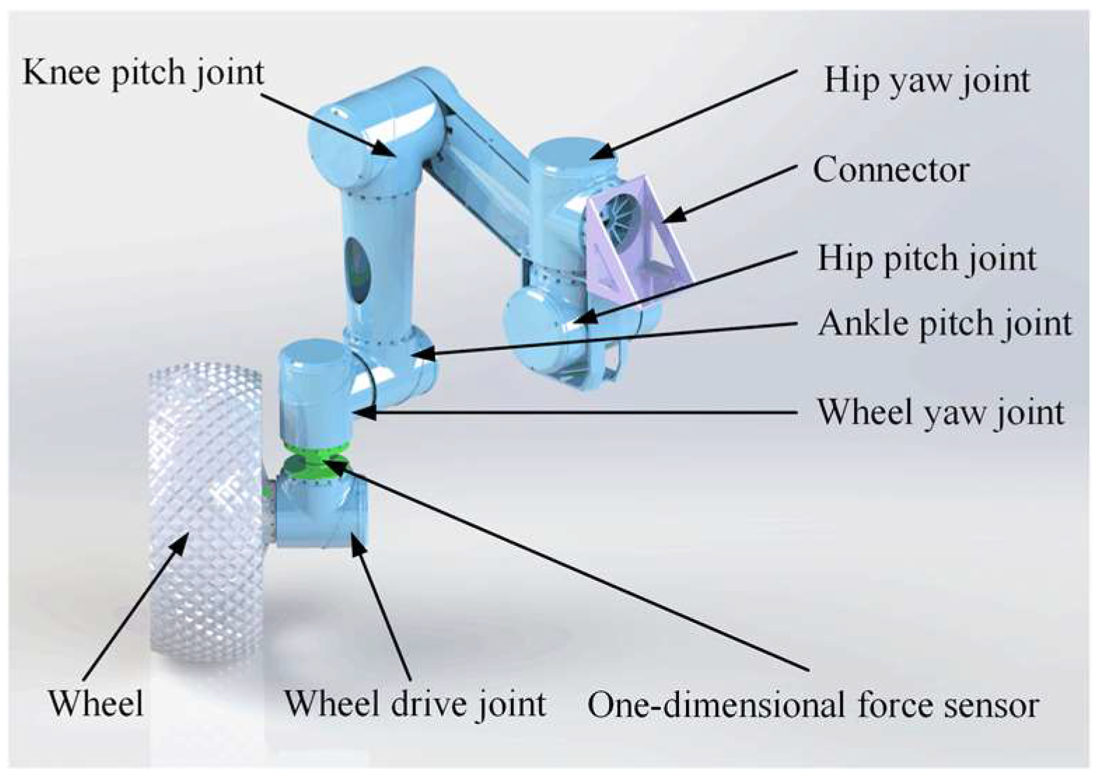The wheel-legged robot has four series legs, which are respectively installed at the four corners of the rectangular body, as shown in Figure 1. Moreover, the wheel-legged robot is equipped with one lidar and one binocular camera to perceive all the information on the environment. Each series leg has six active joints, namely, the hip yaw joint, hip pitch joint, knee pitch joint, ankle pitch joint, wheel yaw joint, and wheel drive joint, as shown in Figure 2. The cooperation of these six joints can actively adjust the spatial position and attitude of the wheel, which can not only carry out foot motion but also effectively improve the performance of the wheeled motion.

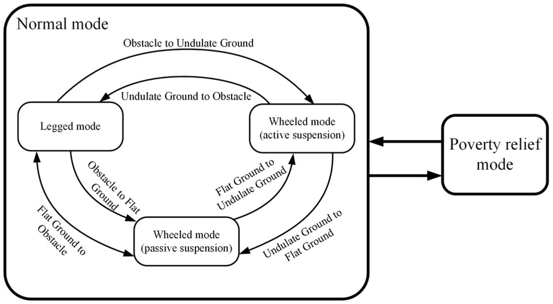
The wheel-legged robot needs to choose the appropriate motion mode according to the terrain conditions. When the terrain is relatively flat, the robot adopts the wheeled motion mode with a passive suspension to improve the efficiency of the roving exploration. In the wheeled motion mode with the passive suspension, the leg configuration remains unchanged, and the body may fluctuate slightly. The leg joints support all the weight of the robot through the internal mechanical lock, which can also reduce energy consumption. When the terrain is undulating, the robot needs to switch to the wheeled motion mode with active suspension, which allows the leg joints to adjust the configuration in time, according to the attitude changes of the body caused by the undulating terrain to ensure stability. When encountering obstacles, such as bumps, pits, and rocks, the wheel-legged robot needs to switch to the legged motion mode to cross the obstacles safely. Due to the unknown terrain conditions, emergencies are very likely to occur. Once the wheel is trapped, the robot can be switched to poverty relief mode to restore the wheel to a safe state. The wheel-legged robot motion mode selection and switching relationships are shown in Figure 3.

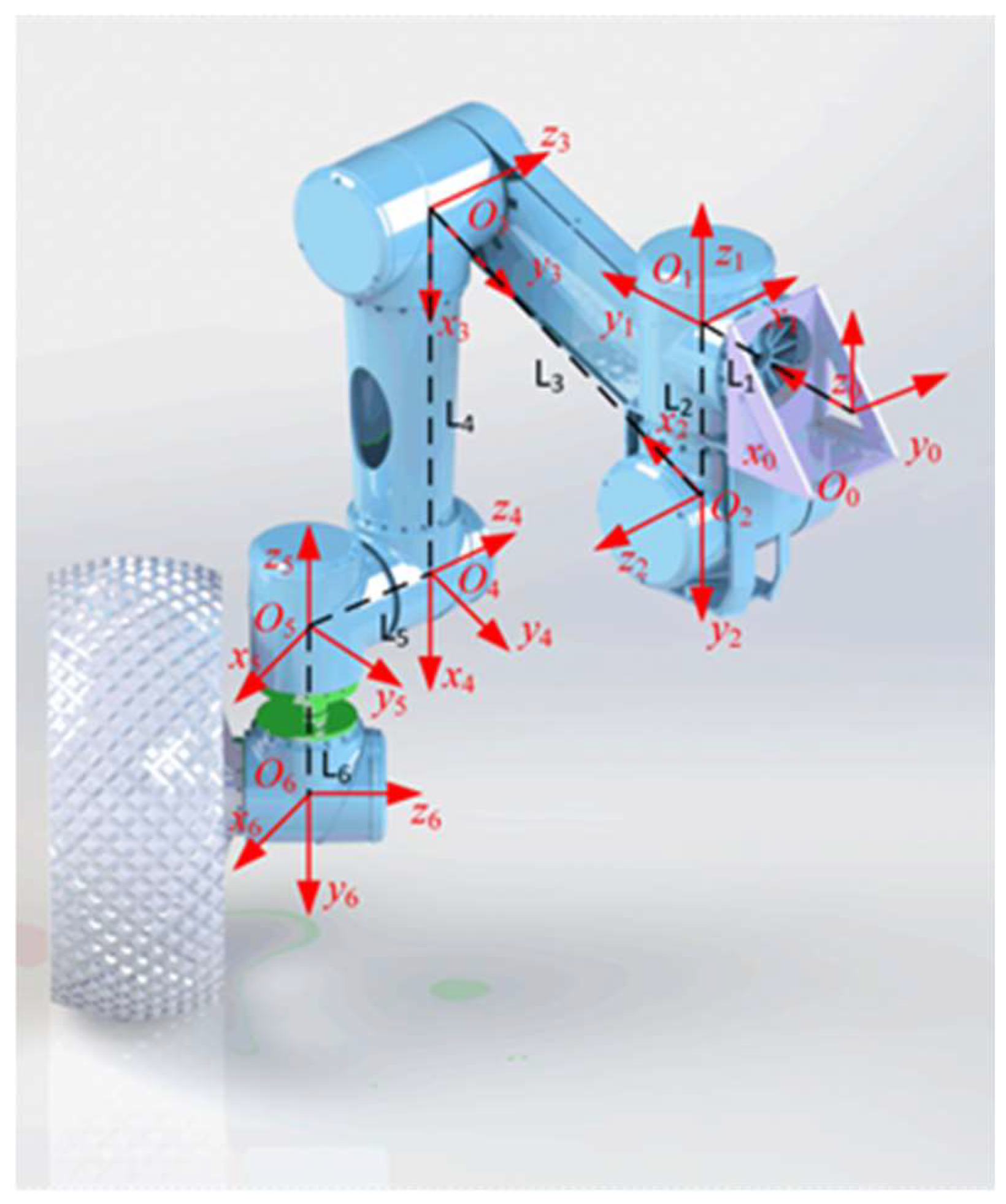
The kinematic model of the single leg establishes the relationship between the joint angles and the position and posture of the wheel, which is of great significance to path planning and motion control. The coordinate system of the single leg is shown in Figure 4.

Since the structure of each leg of the wheel-legged robot is similar, the left front leg is taken as an example to illustrate the kinematic modeling. The coordinate system O₀ is the leg reference coordinate system, of which the origin is located at the intersection of the fixed axis of the hip yaw joint and the outer edge surface of the connector. The axis z₀ takes vertical upward as the positive direction, and the axis x₀ takes horizontal forward as the positive direction. According to the right-hand rule, the positive direction of axis y₀ is shown in Figure 4. On this basis, the coordinate system of the hip yaw joint O₁, the coordinate system of the hip pitch joint O₂, the coordinate system of the knee pitch joint O₃, the coordinate system of the ankle pitch joint O₄, the coordinate system of the wheel yaw joint O₅, and the coordinate system of the wheel drive joint O₆ are established. The L_i is the distance between the origin of the coordinate system O_i-1 and the origin of the coordinate system O_i. The three-dimensional workspace of the wheel can be obtained from the single-leg kinematics model, as shown in Figure 5a. Since the single leg has a hip yaw joint, the projection of the workspace in the horizontal plane is a fan-shaped area, as shown in Figure 5b.

4. The Construction of the Grid Map for the Wheel and Body

Before planning the path, it is necessary to establish a map of the environment based on the point cloud information obtained by the perception system and to distinguish the areas that the robot can pass through, and the areas occupied by obstacles. The grid map describes the environment using grids of the same size, which is simple, effective, and easy to be established. The typical grid map is shown in Figure 6. Grids have two states: occupied state and free state. The white grid indicates the area that can be passed through, which is reflected in the free state, while the black grid indicates the area occupied by obstacles and corresponds to the occupied state.

As the body of the wheel-legged robot is much higher than the wheels, the passability of one area is different for the wheel and body. If the height of one obstacle is greater than that of the body, this obstacle belongs to the impassable area for both body and wheel, which is called the “complete obstacle”. In addition, if the height of one obstacle is lower than that of the body, this obstacle belongs to the passable area for the body, yet belongs to the impassable area of the wheel, which is called the “incomplete obstacle”.

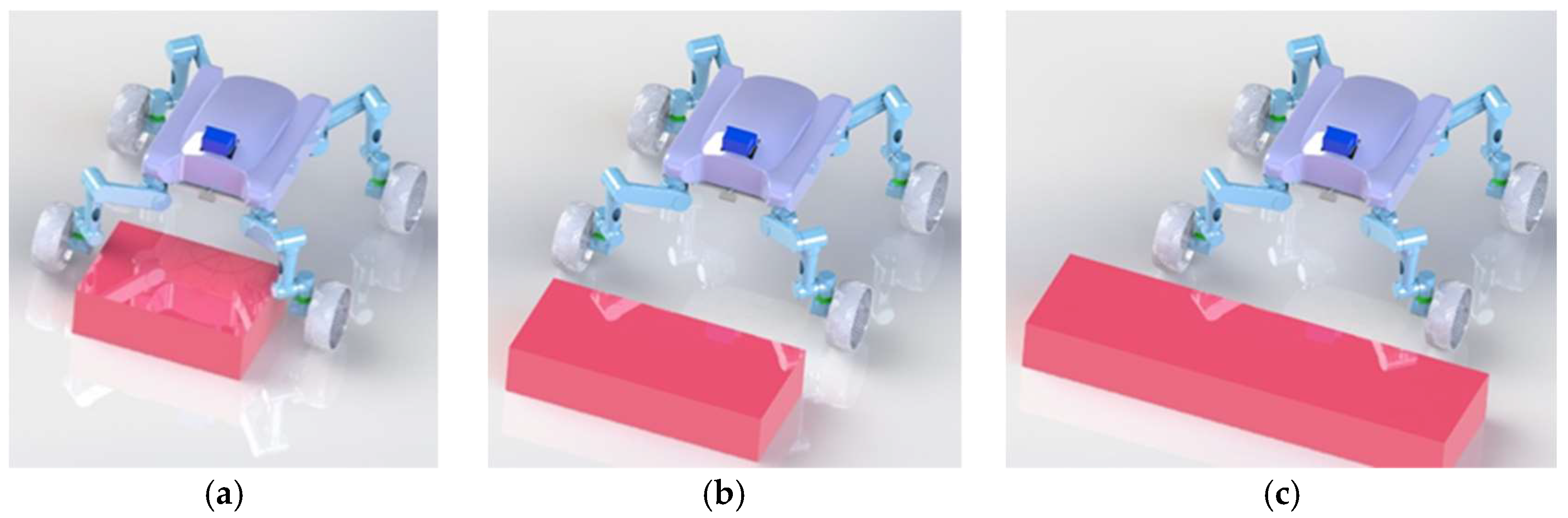
As shown in Figure 7a, the height of the red obstacle is much lower than that of the body. When the robot adopts the configuration shown in the figure, the robot can cross the obstacle safely. The obstacle belongs to the impassable area for the wheel and the passable area for the body, namely, the “incomplete obstacle”. In addition, when the width of the obstacle is larger than the distance between the left wheel and right wheel, the robot can increase the wheel distance to avoid a collision between the wheel and the obstacle, as shown in Figure 7b. However, if the width of the obstacle is too large, the collision between the wheel and the obstacle cannot be avoided after adjusting the configuration, as shown in Figure 7c.

In the roving exploration of the surface of the planet, the wheel-legged robot needs to maintain communication between itself and the communication base station, such as the exploration base, communication satellite, and leader robot. Moreover, some equipment on the exploration robot is sensitive to the orientation and frequent turns will decrease the performance of the equipment. Hence, there is a desire to fix the orientation of the wheel-legged robot. In order to meet the abovementioned requirements, the orientation of the wheel-legged robot is supposed to be fixed in the process of the map construction for the wheel and body.

According to Section 2, the projection of the workspace of the wheel in the horizontal plane is a fan-shaped region. When the body is in a certain position, if the fan-shaped area is completely located in the obstacle area, the wheel cannot avoid collision with the obstacle. Furthermore, as the grid map of the body is generated for the center of the body, when the center of the body is near the obstacle, the edge of the body may collide with the obstacle. Although there is no actual obstacle in the position of the center of the body, the position is still an impassable area for the center of the body. This paper hypothesizes that the position is occupied by a “virtual obstacle”. As shown in Figure 8, the rectangular ABCD represents the body, while point O represents the center of the body. For ease of analysis, the fan-shaped area was simplified to a hexagon AEFGHI, and the red circle represents the obstacle. The relationship between the hexagon AEFGHI and the obstacle area can be approximately judged by calculating the distances from point A, point E, point F, point G, point H, and point I to the center of the circular obstacle. In Figure 8a, the hexagon area is completely within the obstacle area. Hence, the position of the center of the robot body O is considered to be occupied by the virtual obstacle. In Figure 8b, part of the hexagon area is in the red obstacle area, and the collision between the wheel and the obstacle can be avoided by adjusting the leg configuration, meaning it is considered that the position of the center of the robot body O belongs to the feasible area. In Figure 8c, the hexagon area is completely separated from the obstacle area, in which case, the position of the center of the robot body O belongs to a feasible area. Furthermore, the virtual obstacle caused by the collision between the edge of the body and the obstacle can be judged by the distance between the center of the body and the center of the obstacle.

Establishing the grid map for the wheel is simple, whereby the grid inside the obstacles is marked as the occupied state directly. However, establishing the grid map for the body is relatively complex. According to the height of the obstacle, it can be judged whether the obstacle is a complete obstacle or an incomplete obstacle, and the grid is marked inside the complete obstacle as the occupied state, while the grid at the incomplete obstacle is free. On this basis, virtual obstacles should be searched for in the passable area, and the position of the virtual obstacle marked as the occupied state.

To search for virtual obstacles, a grid near the obstacle is taken as the position of the center of the body, and the distances from the vertexes of the hexagon area to the center of the obstacle are calculated. The relative position between the hexagon region and the obstacle can be obtained. It can be judged whether it is the position occupied by the virtual obstacle. Taking all the grids near the obstacle as the position center of the robot body, all the areas occupied by the virtual obstacle can be searched.

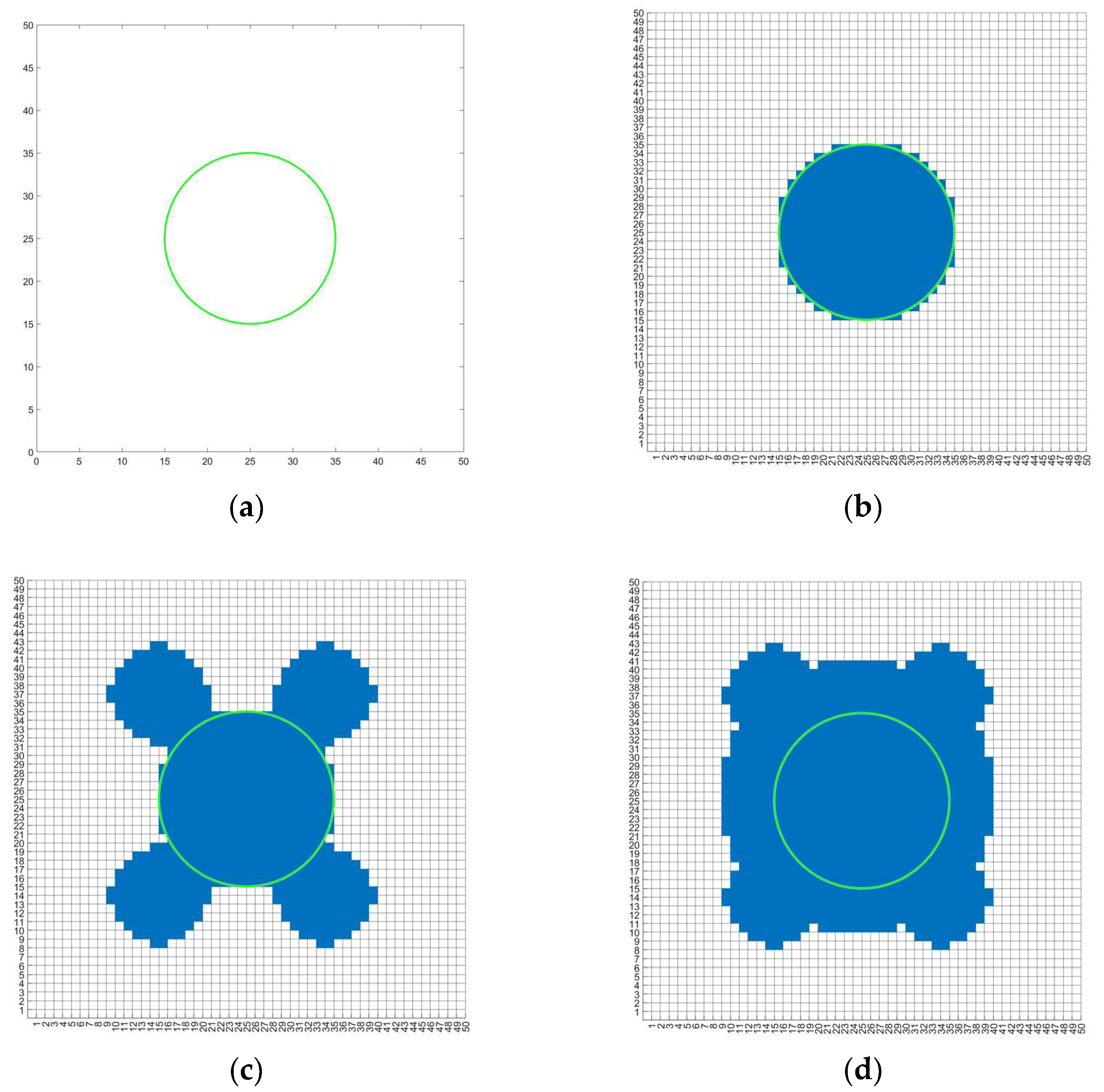
As shown in Figure 9a, a circular complete obstacle is located in the center of a 50 × 50 cell grid mapping the scenario, the position of the center is (25,25) and the radius is r = 10. The outline of the obstacle is represented by a green circle. When generating a grid map for the body, the state of the grid is first set within the circular area to the occupied state to obtain an original grid map, as shown in Figure 9b, and then, the area occupied by the virtual obstacle is identified. Merging the abovementioned two kinds of obstacle areas can provide the grid map for the body, as shown in Figure 9c.

In addition, since the incomplete obstacle is still impassable for the wheels, it is also necessary to search the virtual obstacle area near the incomplete obstacle. As shown in Figure 10a, an incomplete obstacle is located in the center of the grid map, with a red circle representing the outline of the obstacle. The area occupied by the incomplete obstacles is a passable area for the robot body, meaning there is no change when generating the original grid map, as shown in Figure 10b. The grid map for the body can be generated finally by searching for a virtual obstacle, as shown in Figure 10c. When the geometric center of the robot body is located, in the blue area in the picture, the robot wheel will inevitably interfere with the obstacle.

As shown in Figure 11a, there are two obstacles. The green circle represents a complete obstacle, while the red circle represents an incomplete obstacle. For the two types of obstacles, the grid maps for the wheels and the grid map for the body are generated, as shown in Figure 11b and Figure 11c, respectively. The impassable area of the wheel is composed of two obstacles, while the impassable area of the body is composed of a virtual obstacle and a complete obstacle.

Using grid maps for the body and wheels, the path of the body and the path of the wheels are planned in different maps. As the grid map for the body is generated by taking the center of the body as the main analysis object, the wheel-legged robot can be simplified as a point in the grid map for the body, which can reduce the difficulty of path planning significantly.

As the wheel-legged robot is symmetrical, the area of the virtual obstacle is symmetrical about the symmetrical obstacle. According to the characteristic of symmetry, the map can be checked intuitively, which can help ensure the safety of the wheel-legged robot.

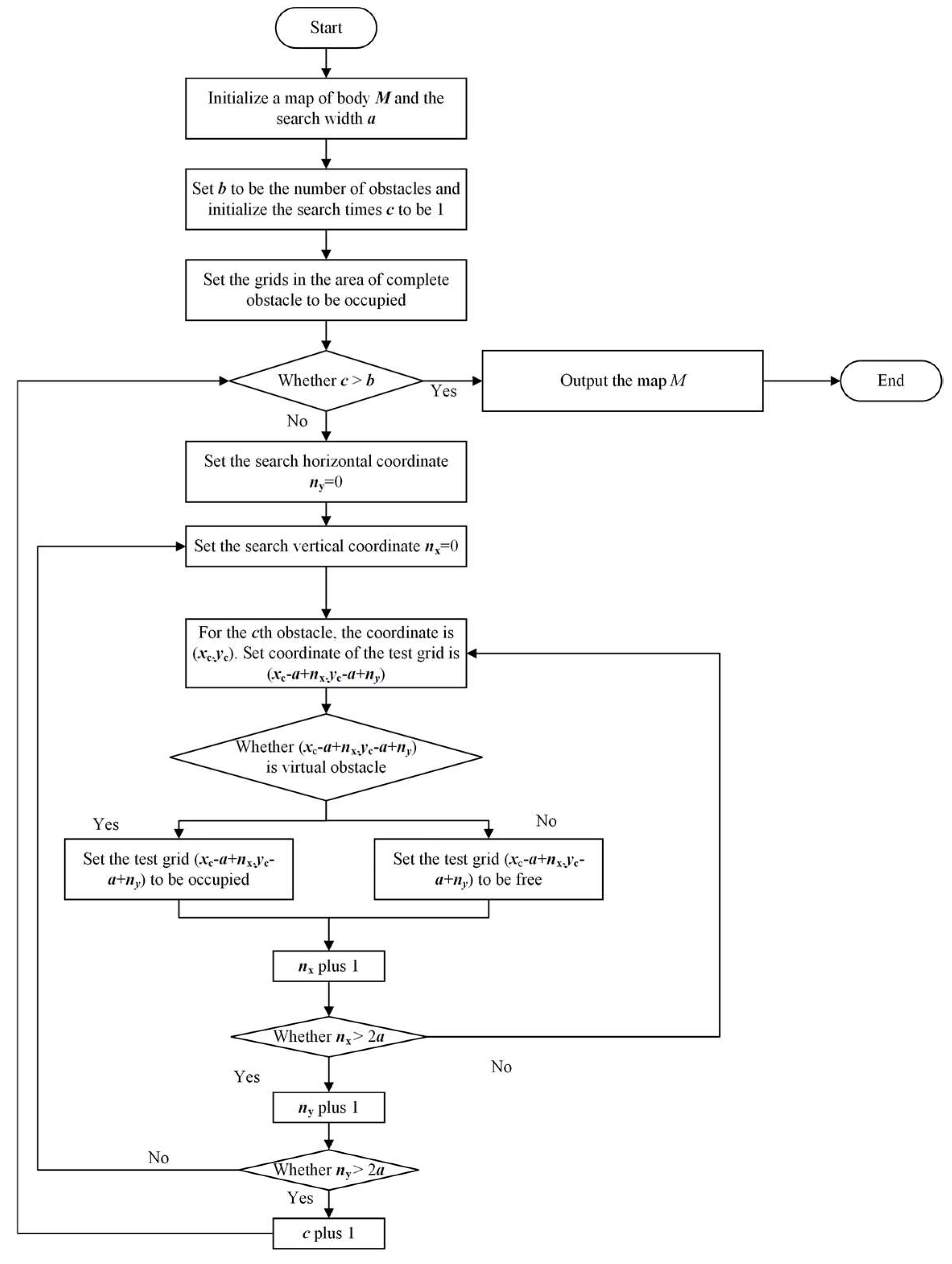
The flowchart for generating the map of the body is shown in Figure 12. The process of generating the map of the wheel is relatively simple and the flowchart is not provided in this paper.

5. Path Planning Based on the Theta* Algorithm and TEB Algorithm

5.1. Global Path Planning of Body Based on the Theta* Algorithm

The Theta* algorithm is a classical heuristic algorithm in global path planning and one of the most effective algorithms for finding the shortest path. The Theta* algorithm uses the cost function f (n) to calculate the priority of each node during each expansion. The node with the lowest f (n) value among the 8 nodes around each expansion is retained, and the search is continued until reaching the target node. The cost function f (n) is shown in Equation (1).

$$f\left(n\right)=g\left(n\right)+h\left(n\right)$$

(1)

where n represents the current node, g (n) represents the actual cost value from the start node to the current node, and h (n) represents the estimated cost value from the current node to the target node. In this paper, the actual cost value g (n) is calculated by Euclidean distance, as shown in Equation (2).

$$g\left(n\right)=\sqrt{{\left(x_n-x_{initial}\right)}^2+{\left(y_n-y_{initial}\right)}^2}$$

(2)

where x_n and y_n denote the horizontal coordinate and vertical coordinate of the current node, and x_initial and y_initial denote the horizontal coordinate and vertical coordinate of the start node, respectively.

Here, h (n) is an important part of the heuristic cost function, which has an important influence on the efficiency of path planning. The smaller the h (n) value, the more nodes the Theta* algorithm will expand, which can guarantee to find the shortest path, although it will greatly increase the search time. The larger the h (n) value, the faster the Theta* algorithm searches, yet there is no guarantee that the shortest path can be found. In this paper, the weighted Euler distance is used as the estimated cost function, as shown in Equation (3).

$$h\left(n\right)=H\times \sqrt{{\left(x_n-x_{goal}\right)}^2+{\left(y_n-y_{initial}\right)}^2}$$

(3)

where H is the weight, and x_goal and y_goal are the horizontal coordinates and vertical coordinates of the target node, respectively. Compared to the A* algorithm, the Theta* algorithm adds a preliminary visibility check, which requires the visibility check of the current node’s parent node and its successor node during expansion. If the direct connection between a parent node and the successor node does not pass through the obstacle and the cost is lower, the parent node of the successor node is set as the parent node of the current node. Otherwise, the parent node of the successor node is set as the current node. The steps of the Theta* algorithm to search the path are as follows.

(1)

Initialize the start point and target point, create a new OPEN table and CLOSE table, and add the start point (x_initial, y_initial) to the OPEN table.

(2)

Judge whether the OPEN table is empty. If so, planning fails, and the search is terminated. Otherwise, take the node in the OPEN table with the lowest evaluation cost as the current node to be expanded and set it to n.

(3)

Judge whether node n is the target point. If so, the path has been planned successfully, and backtrack all nodes along the path. Otherwise, go to the next step.

(4)

Expand node n. Traverse all neighborhood nodes of node n (set to p) and do the following:

a.

If node p is an obstacle or is already in the CLOSE table, no processing is made. Otherwise, proceed to the next step.

b.

Check whether the parent node of node n exists. If it does not exist, record node n. Otherwise, determine whether the parent node of node p and node n is visible. If visible, record the parent node of node n, otherwise record node n. Name the node of the final record node k, and then proceed to the next step.

c.

If node p is not in the OPEN table, add it to the OPEN table, and set the parent node of node p to node k. Finally, calculate the cost of node p. If node p is already in the OPEN table, judge whether the cost of passing node k is lower than the original cost. If so, change the parent node of node p to node k and update the cost of node p. If not, do not conduct any processing.

(5)

Remove node n from the OPEN table, then, add it to the CLOSE table. Return to step (2). The flowchart of the Theta* algorithm is shown in Figure 13.

5.2. Path Smoothing and Optimization Based on the TEB Algorithm

In this paper, the TEB algorithm is used to smooth and re-optimize the original path obtained by the Theta* algorithm under constraints. Each point along the original path can be represented as a state of the robot, which is marked as q_i. The robot state in the two-dimensional map can be represented by the robot’s position and yaw angle, as shown in Equation (4).

$$q_i=\left[x_i,y_i,{\theta }_i\right]$$

(4)

where x_i, y_i, and θ_i denote the horizontal coordinate, vertical coordinate, and yaw angle of the i-th node along the original path, respectively. All the w states form a state sequence Q, as shown in Equation (5).

$$Q=\left\{q_i\right\},i=1,2,\dots ,w$$

(5)

ΔT_i is defined as the time interval between the current state q_i and the next configuration q_i+1. Hence, all time intervals form a time sequence τ, as shown in Equation (6).

$$\tau =\left\{\Delta T_i\right\},i=1,2,\dots ,w$$

(6)

with the combination of the state sequence and the time sequence, the points along the original path can be expressed as the robot state sequence based on the time step, as shown in Equation (7).

$$B=\left\{Q,\tau \right\}$$

(7)

the optimal path time and tracking original path point constraint, obstacle avoidance constraint, velocity constraint, acceleration constraint, and minimum turning radius constraint are quantified to establish a weighted multi-objective optimization function, as shown in Equation (8).

$$F\left(B\right)={\displaystyle \sum _{k=1}^t{\eta }_k{f}_k}$$

(8)

where η_k is the weight of the k-th cost function and t is the number of cost functions. The optimization goal is to find a sequence B* to minimize the optimization function F (B), as shown in Equation (9).

$$B^{*}=\arg \min F\left(B\right)$$

(9)

constraints of the TEB algorithm can usually be divided into two categories: punitive constraints of the robot deviating from the global path and near the obstacle, and normal constraints caused by velocity, acceleration, minimum turning radius, etc.

(1)

The objective function of time optimization.

In this paper, the shortest time to pass through the whole path is taken as the optimization objective. Hence, the sum of the squares of all the time intervals is taken as the optimal quantization function of time, as shown in Equation (10).

$$f_t={\displaystyle \sum _{i=1}^w\Delta T_i{}^2}$$

(10)

(2)

Constraint of following the original path point.

In Section 5.1, the original path points have been planned using the Theta* algorithm. Although the accuracy of the original path points was relatively low and there were many turning points, the original path points had important guiding significance for path smoothing and re-optimization. The TEB takes the original path points as an important constraint so that the smoothed and optimized path can follow the original path as much as possible. By traversing all the original path points, the nearest original path point to the TEB state can be found. The distance is marked as d_i. By summing all the distances, the cost function of deviating from the original path point can be obtained, as shown in Equation (11).

$$f_q={\displaystyle \sum _{i=1}^w{d}_i}$$

(11)

(3)

Constraint of avoiding the obstacle.

When using the TEB to smooth and optimize the original path, it is necessary to avoid a collision between the robot and the obstacles. In the optimization objective function, the cost function caused by avoiding obstacles is shown in Equation (12).

$$f_o=\left\{\begin{array}{cc}0& ,d_o>d_{\min }\\ {\left(d_0-d_{\min }\right)}^2& ,d_0\le d_{\min }\end{array}\right.$$

(12)

where d_o is the distance between the current position and the obstacle, and d_min is the minimum safe distance between the robot body and the obstacle.

(4)

Constraints of velocity and angular velocity.

The motion velocity and angular velocity of the robot can be approximately calculated by the Euclidean distance and the yaw angle between two adjacent states, as shown in Equation (13).

$$\left\{\begin{array}{l}{v}_i=\frac{1}{\Delta T_i}‖\begin{array}{c}{x}_{i+1}-x_i\\ y_{i+1}-y_i\end{array}‖=\frac{\sqrt{{\left(x_{i+1}-x_i\right)}^2-{\left(y_{i+1}-y_i\right)}^2}}{\Delta T_i}\hfill \\ w_i=\frac{{\theta }_{i+1}-{\theta }_i}{\Delta T_i}\hfill \end{array}\right.$$

(13)

The cost functions caused by the velocity constraint and the angular velocity constraint in the objective function are shown in Equations (14) and (15).

$$f_v=\left\{\begin{array}{cc}0& ,v\le v_{\max }\\ {\left(v-v_{\max }\right)}^2& ,v>v_{\max }\end{array}\right.$$

(14)

$$f_w=\left\{\begin{array}{cc}0& ,w\le w_{\max }\\ {\left(w-w_{\max }\right)}^2& ,w>w_{\max }\end{array}\right.$$

(15)

where v_max and θ_max are the maximum velocity and angular velocity, respectively.

(5)

Constraints of acceleration and angular acceleration.

The acceleration and angular acceleration of the robot can be obtained by taking further differentiation of the velocity, as shown in Equation (16).

$$\left\{\begin{array}{l}{a}_i=\frac{2\left(v_{i+1}-v_i\right)}{\Delta T_{i+1}+\Delta T_i}\hfill \\ b_i=\frac{2\left(w_{i+1}-w_i\right)}{\Delta T_{i+1}+\Delta T_i}\hfill \end{array}\right.$$

(16)

whereby the cost functions caused by the acceleration constraint and angular acceleration constraint in the objective function are shown in Equations (17) and (18).

$$f_a=\left\{\begin{array}{cc}0& ,a\le a_{\max }\\ {\left(a-a_{\max }\right)}^2& ,a>a_{\max }\end{array}\right.$$

(17)

$$f_b=\left\{\begin{array}{cc}0& ,b\le b_{\max }\\ {\left(b-b_{\max }\right)}^2& ,b\le b_{\max }\end{array}\right.$$

(18)

where a_max and b_max are the maximum acceleration and angular acceleration, respectively.

(6)

Constraint of minimum turning radius.

Although the wheel-legged robot can steer in place, in-place steering requires the robot to be paused, which decreases the exploration efficiency. Therefore, the minimum turning radius constraint is added to reduce the turning point and improve the smoothness of the path. The turning radius can be approximately obtained from the velocity and angular velocity, as shown in Equation (19).

$$r_i=\left|\frac{v_i}{w_i}\right|$$

(19)

hence, the cost function caused by the minimum turning radius is shown in Equation (20).

$$f_r=\left\{\begin{array}{cc}0& ,r\ge r_{\min }\\ {\left(r-r_{\min }\right)}^2& ,r<r_{\min }\end{array}\right.$$

(20)

where r_min is the minimum turning radius of the robot.

Owing to the sparse structure of the optimization problem, the B(Q,τ) sequence can be solved optimally by using the graph optimization theory. Taking the state q_i and the time interval ΔT_i as the node of the graph, and by taking the velocity constraint, acceleration constraint, tracking the path point constraint, avoiding the obstacle constraint, and using the minimum turning radius constraint as the edges of the graph, the hypergraph optimization can be constructed, as shown in Figure 14. The general graph optimization framework G2O is used to solve the hypergraph, and the optimized sequence can be obtained.

5.3. Path Planning for the Wheel

The wheel-legged robot can adjust the leg configuration according to the terrain condition; therefore, it is necessary to plan the path of the wheel after planning the path of the robot body. Once the final path of the robot body is determined, the feasible area of the wheel will be limited to a certain area around the robot body. The workspace of the wheel at the end of the leg is approximately a fan-shaped area. The length l and the angle α between the wheel and the center of the fan-shaped area can be used to represent the position of the wheel, as shown in Figure 15. The yellow circle indicates the position of the wheel.

Since the structural size of the body is fixed, the position of the fan-shaped area center relative to the center of the body remains unchanged. In this paper, it is stipulated that the configuration of the robot is a nominal configuration when l = 0.3 m, α = 45°. The robot moves with the nominal configuration in most cases. When the robot needs to adjust the configuration to adapt to the obstacle, the robot searches for the feasible position of the wheel by changing the length l and the angle α. The steps to search for a feasible position of the wheel are as follows:

(1)

Initialize the length and adjust n₁ times as 0.

(2)

Initialize the angle and adjust n₂ times as 0.

(3)

Set the length l fixed and adjust the angle α according to Equation (21) and n₂ plus 1.

$${\alpha }_{n+1}={\alpha }_0+{(-1)}^{n_2}{n}_2$$

(21)

(4)

Judge whether the wheel interferes with the obstacle. If not, the feasible wheel position has been searched successfully. Otherwise, proceed to the next step.

(5)

Judge whether n₂ is greater than the threshold. If not, go to Step (3). Otherwise, proceed to the next step.

(6)

Adjust the length l according to Equation (22) and n₁ plus 1.

$$l_{n+1}=l_0+0.1\times {(-1)}^{n_1}{n}_1$$

(22)

judge whether n₁ is greater than the threshold. If not, go to Step (2). Otherwise, the search failed. The flowchart for searching for the feasible position of the wheel is shown in Figure 16.

6. Simulations

To verify the effectiveness of the proposed path planning algorithm, this section simulates and analyzes the algorithm for the different types of obstacles with Matlab 2022 b. The main structural parameters of the wheel-legged robot in the simulation are shown in

Table 1. Main structural parameters of the wheel-legged robot.

Name	Value
Width of body	0.6 m
Length of body	0.8 m
Height of body	0.6 m
Radius of fan-shaped wheel workspace	0.6 m
Center angle of fan-shaped wheel workspace	90°
Maximum velocity	0.5 m.s−1
Maximum angular velocity	0.05 rad.s−1
Maximum acceleration	0.1 m.s−2
Maximum angle acceleration	0.01 rad.s−2
Minimum turning radius	0.7 m
Minimum safe distance between robot and obstacle	0.1 m

.

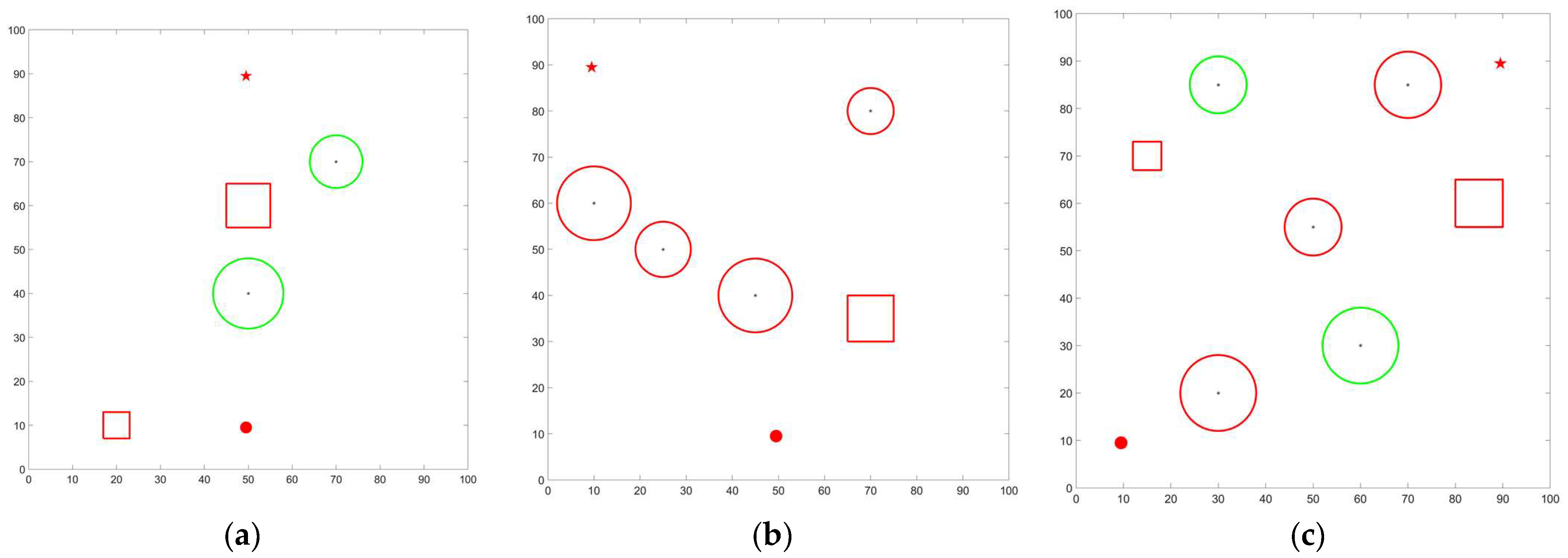
According to the structural parameters shown in Table 1, this paper takes an area of 10 m × 10 m as the example. Taking 0.1 m as the edge length of the grid means a grid map with a size of 100 × 100 can be obtained. In the following figures, the horizontal axis and the vertical axis are the number of grids. In order to simplify the figure, the grid numbers of two axes are shown at intervals of 10. To verify the feasibility of the proposed algorithm for different types of obstacles, three types of grid maps are set up in the simulation. In the first map, all the obstacles are complete obstacles, represented by green circles, as shown in Figure 17a. In the second map, all the obstacles are incomplete obstacles, represented by red circles, as shown in Figure 17b. The third map consists of a mixture of complete obstacles and incomplete obstacles, with green circles representing complete obstacles and red circles representing incomplete obstacles, as shown in Figure 17c. In addition, the solid red circle represents the start point, and the solid red five-pointed star represents the target point.

6.1. The Simulation of the M1 Map

According to Section 3, the grid map for the wheel and the body of M1 can be generated as shown in Figure 18, where the yellow grids are the impassable area. As shown in Figure 18a, the obstacle area for the wheels consists of two circular complete obstacles and two rectangular incomplete obstacles. As shown in Figure 18, the obstacle area for the robot body consists of the area occupied by two complete obstacles and the area occupied by a virtual obstacle. In order to highlight key components in the map, such as the start point, target point, obstacle, path, etc., the gridline is not displayed in the following Figures.

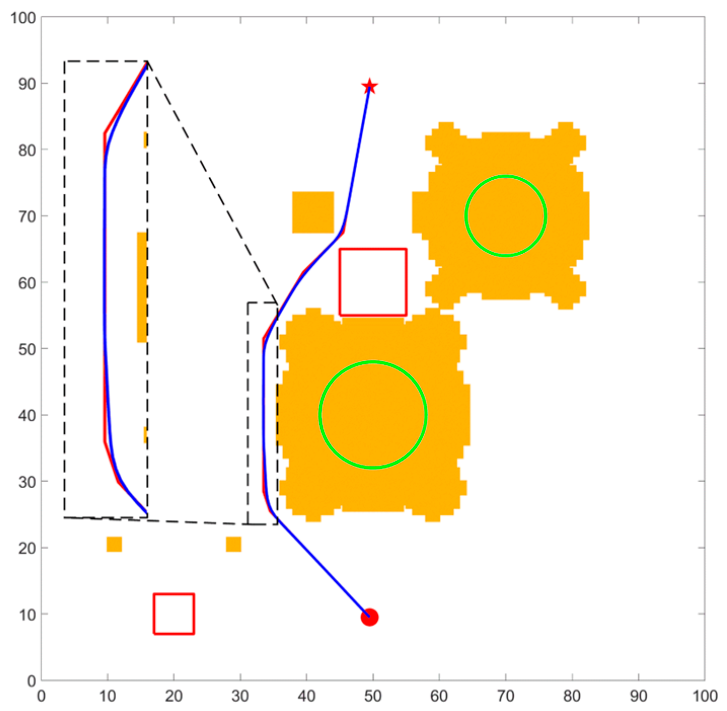
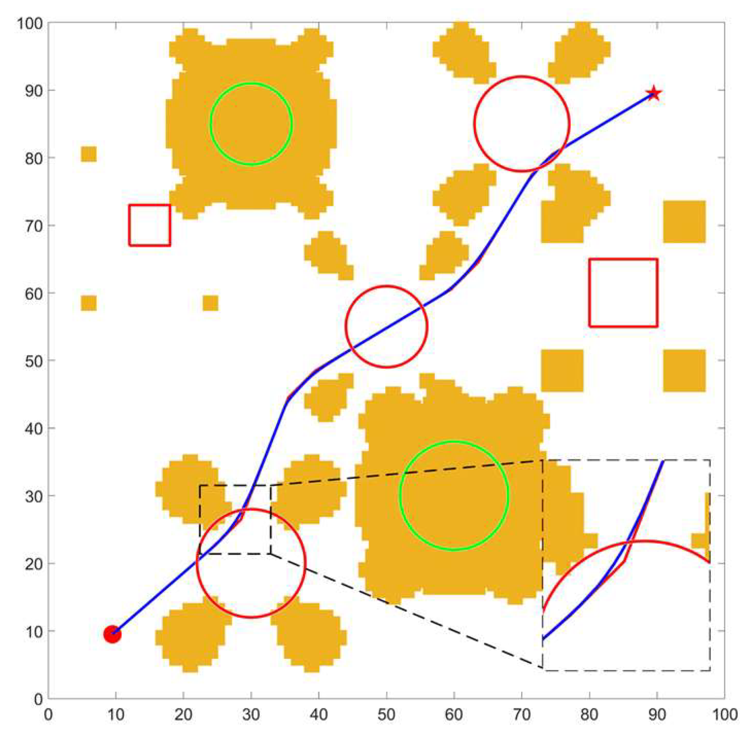
After obtaining the grid map for the wheel and body, the original path of the body is planned using the Theta* algorithm and TEB algorithm, as shown in Figure 19. In Figure 19, the red line is the original path obtained by the Theta* algorithm and the blue line is the optimized path obtained by the TEB algorithm. The two lines almost coincide except at the turns of the original path. From Figure 19, it can be seen that the robot first moves in a straight line to the left safe area. After that, the robot moves vertically until it leaves the obstacle, and finally, it moves to the upper right to reach the target point. The robot body successfully bypasses the obstacle area and ensures its safe movement, although there are four turning points in the original path, where the robot needs to pause its motion and change the direction of its body. After smoothing and re-optimizing with the TEB algorithm, the final path of the body is generally consistent with the original path. It can be seen from the enlarged view that the original turning point has been smoothed into a curve. Hence, the robot can perform continuous and smooth steering movements. According to Section 5.3, the path of the wheel can be obtained according to the body path, as shown in Figure 20. From the enlarged view in Figure 20, the right rear wheel can bypass the rectangular obstacle closely and safely to decrease the length of the path, in general.

6.2. The Simulation of the M2 Map

As shown in Figure 21, the grid maps for the body and wheel are generated from the M2 map. As shown in Figure 21a, the obstacle area of the wheel consists of four circular incomplete obstacles, each with a different radius, and one rectangular incomplete obstacle. As shown in Figure 21b, the obstacle area of the body only consists of virtual obstacles.

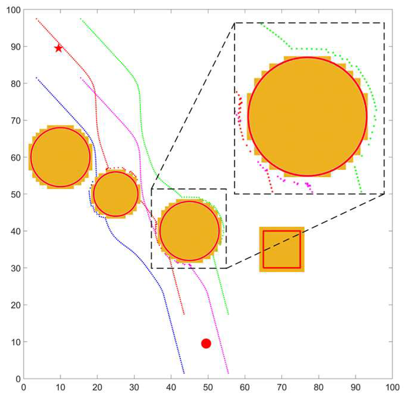
The original path of the body is planned with the Theta* algorithm in the M2 map, which is the red line, as shown in Figure 22. The robot bypasses the virtual obstacle area and crosses over the middle incomplete obstacle. However, there are many turning points to change the direction of the robot. After further smoothing and re-optimization of the original path with the TEB algorithm, the final path is the blue line shown in Figure 22. The final path is consistent with the original path in general, keeping a safe distance from the obstacle area. Furthermore, the original turning point has been transformed into a curve, as shown in the enlarged view. According to Section 5.3, the path of the wheel, as shown in Figure 23, can be obtained according to the robot’s body path. When the robot body passes over the middle incomplete obstacle, the four wheels detour around the incomplete obstacle to shorten the path length, while ensuring safe movement, as shown in the enlarged view in Figure 23.

6.3. The Simulation of the M3 Map

In the M3 map, the grid maps for the body and wheel are shown in Figure 24. As shown in Figure 24a, the obstacle area of the wheels consists of two circular complete obstacles, three circular incomplete obstacles, and two rectangular incomplete obstacles. As shown in Figure 24b, the obstacle area of the body consists of virtual obstacles and complete obstacles.

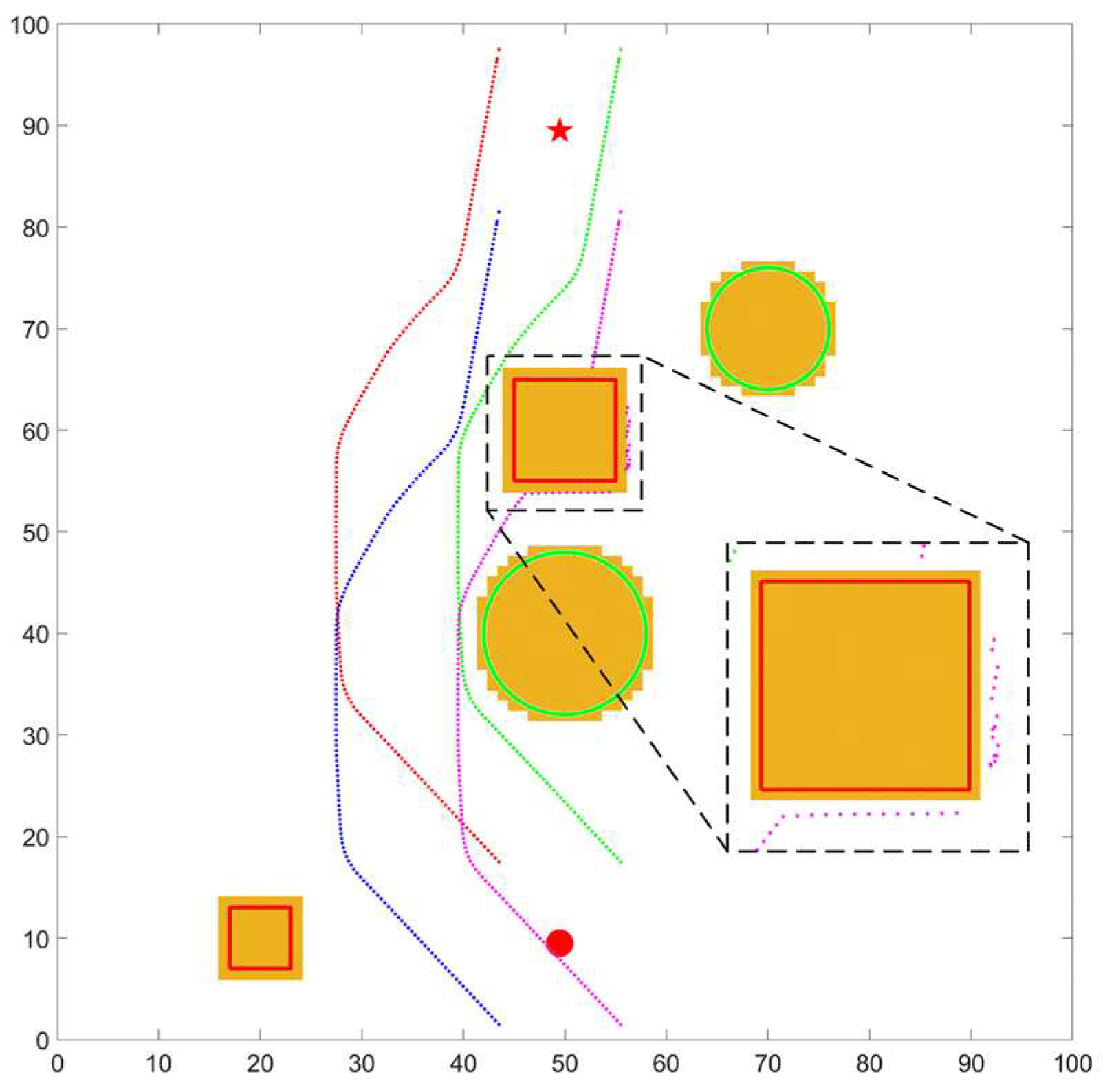
The original path of the body is planned using the Theta* algorithm, as the red line shown in Figure 25. The robot crosses over three incomplete obstacles to the target point while avoiding interference by the virtual obstacle area. When passing through an area composed of a variety of obstacles, the robot can choose the passing strategy for different obstacles. The detour method is adopted for the complete obstacle and the virtual obstacle, and the method of crossing above is adopted for the incomplete obstacle. Smoothing and re-optimization of the original path were carried out using the TEB algorithm. The blue line shown in Figure 25 demonstrates that the final path is generally consistent with the original path and maintains a safe distance from the obstacle area, thereby ensuring the safety of the robot’s movement. The original turning points have also been smoothed into a curve. According to Section 5.3, the path of the wheel, as shown in Figure 26, can be obtained. When the robot body crosses over the incomplete obstacle in the middle of the map, four wheels detour around the incomplete obstacle to ensure its safe movement, while shortening the path length.

6.4. Comparisons

The algorithm proposed in this paper makes some contribution to generating the map for the wheel and body and adopts the Theta* algorithm and TEB algorithm without any significant modification to the planning of the path. Comparisons between the traditional map generation algorithm and the algorithm proposed in Section 4 in the M1, M2, and M3 maps were carried out and the paths were planned with the Theta* algorithm. The wheel-legged robot was simplified as a single point in the traditional Theta* algorithm. Hence, the obstacles were inflated according to the size of the wheel-legged robot to avoid any collisions between the obstacles and the wheel-legged robot. The grid maps for the body in M1, M2, and M3 using the traditional Theta* algorithm are shown in Figure 27. As shown in Figure 27a,b, the area between the start point and the target point is not blocked completely, and a feasible path can be planned. On the contrary, the area between the start point and the target point is blocked completely and no feasible path can be planned (Figure 27c).

For the M1 and M2 maps, the traditional Theta* algorithm was used to search for a feasible path from the start point to the target point. The paths planned by the traditional Theta* algorithm are shown in Figure 28. As can be seen in Figure 28, two paths bypass all obstacles. The length of the path in Figure 28a is 9.71 m, while the length of the original path in the M1 map, obtained by the algorithm proposed in this paper, is 9.06 m, as shown in Figure 19. The average length of the four leg paths for the traditional Theta* algorithm is 9.71 m, while that of the proposed algorithm is 9.25 m. Moreover, the length of the path in Figure 28b is 15.70 m, while the length of the path in the M2 map, in Figure 22, is 9.1 m. The average length of the four paths for the wheels using the traditional Theta* algorithm is 15.70 m, while that of the proposed algorithm is 9.69 m. Hence, the algorithm proposed in this paper can be adapted for more situations and provided better performance in planned path length than the traditional algorithm. Furthermore, the computation time for planning the path in Figure 28a was 16.8s, while in Figure 19 it was 14.3 s. Additionally, the computation time for planning the path in Figure 28b was 58.0 s, while in Figure 22 it was 14.8 s. Hence, the algorithm proposed in this paper provided a better planning efficiency than the traditional Theta* algorithm, to some extent.

6.5. Analysis and Discussion

Through the simulations of the M1, M2, and M3 maps, it can be seen that the path planning algorithm proposed in this paper can plan the path of a wheel-legged robot considering its variable configuration in different scenarios. The map of the body and the map of the wheels can be generated to make the free area more accurate for path planning of the body. For different obstacles, the body can choose different strategies to optimize the path. After smoothing using the TEB algorithm, the turning points were replaced by curves to improve the efficiency of the wheel-legged robot. On that basis, the path of the wheel was searched for.

Furthermore, the comparisons between the path planning algorithm proposed in this paper and the traditional Theta* algorithm were carried out. It can be seen that the path planning algorithm proposed in this paper can avoid the overexpansion of the obstacle and provide a more accurate free space. Moreover, the paths planned by the path planning algorithm were shorter than those of the traditional Theta* algorithm and required less planning time. The path-planning algorithm proposed in this paper is more suitable for the wheel-legged robot.

7. Conclusions

In this paper, a path planning algorithm based on the Theta* algorithm and TEB algorithm was proposed considering variable configuration during the wheeled motion of the wheel-legged robot. Firstly, the structure of the wheel-legged robot, which is the main research object, was introduced and the kinematic model of a single leg was established. Secondly, a method was proposed to judge both complete obstacles and incomplete obstacles according to the height of the obstacles and to search for virtual obstacles of the body according to the relative position between the robot and the obstacles. Grid maps for the wheel and body were established. Then, the original path of the body was planned based on the Theta* algorithm, and the original path was smoothed and re-optimized based on the TEB algorithm, considering the constraints of the robot’s velocity, acceleration, running time, and minimum turning radius, which effectively reduces the turning points in the original path and realizes the hierarchical planning and multiple optimizations of the path. Finally, the proposed algorithm was simulated in three maps. The simulation results show that the algorithm proposed in this paper can effectively plan the path of the wheel-legged robot in different types of maps. It can be realized that detouring around the complete obstacles with the minimum distance and crossing over incomplete obstacles is of great significance to give full play to the advantages of the wheel-legged robot with variable configuration. Through the comparison between the algorithm proposed in this paper and the traditional Theta* algorithm, it can be found that the algorithm proposed in this paper can be adopted in more scenarios and has better performance of computation time and path length.

There are some differences between simulation and experimental tests such as the visual sensor accuracy and computer performance. Once the scenario is mapped, the algorithm can be utilized to path plan, while the performance on the path length was approximately the same. However, the planning time may be different between the simulation and the experiment. In the future, the path planning algorithm will be improved to adapt to more complex and rugged terrains, combining wheeled motion and legged motion. The analysis of the computation time will be executed in detail to modify the algorithm and improve the performance of the computation time. Furthermore, the prototype of the wheel-legged robot will also be developed to carry out verification experiments.

References

1. Kashiri, N.; Baccelliere, L.; Muratore, L.; Laurenzi, A.; Ren, Z.; Hoffman, E.M.; Kamedula, M.; Rigano, G.F.; Malzahn, J.; Cordasco, S.; et al. Centauro: A hybrid locomotion and high power resilient manipulation platform. IEEE Robot. Autom. Lett. 2019, 4, 1595–1602. [Google Scholar] [CrossRef]
2. Reid, W.; Fitch, R.; Göktoğan, A.H.; Sukkarieh, S. Sampling-based hierarchical motion planning for a reconfigurable wheel-on-leg planetary analogue exploration rover. J. Field Robot. 2020, 37, 786–811. [Google Scholar] [CrossRef]
3. Bjelonic, M.; Sankar, P.K.; Bellicoso, C.D.; Vallery, H.; Hutter, M. Rolling in the deep–hybrid locomotion for wheeled-legged robots using online trajectory optimization. IEEE Robot. Autom. Lett. 2020, 5, 3626–3633. [Google Scholar] [CrossRef]
4. Townsend, J.; Biesiadecki, J.; Collins, C. ATHLETE mobility performance with active terrain compliance. In Proceedings of the 2010 IEEE Aerospace Conference, Big Sky, MT, USA, 6–13 March 2010; pp. 1–7. [Google Scholar]
5. Reid, W.; Emanuel, B.; Chamberlain-Simon, B.; Karumanchi, S.; Meirion-Griffith, G. Mobility mode evaluation of a wheel-on-limb rover on glacial ice analogous to europa terrain. In Proceedings of the 2020 IEEE Aerospace Conference, Big Sky, MT, USA, 7–14 March 2020; pp. 1–9. [Google Scholar]
6. Roehr, T.M.; Cordes, F.; Kirchner, F. Reconfigurable integrated multirobot exploration system (RIMRES): Heterogeneous modular reconfigurable robots for space exploration. J. Field Robot. 2014, 31, 3–34. [Google Scholar] [CrossRef]
7. Cordes, F.; Kirchner, F.; Babu, A. Design and field testing of a rover with an actively articulated suspension system in a Mars analog terrain. J. Field Robot. 2018, 35, 1149–1181. [Google Scholar] [CrossRef]
8. Wang, C.N.; Yang, F.C.; Vo, N.T.M.; Nguyen, V.T.T. Wireless communications for data security: Efficiency assessment of cybersecurity industry—A promising application for UAVs. Drones 2022, 6, 363. [Google Scholar] [CrossRef]
9. Chen, M.; Sharma, A.; Bhola, J.; Nguyen, T.V.T.; Truong, C.V. Multi-agent task planning and resource apportionment in a smart grid. Int. J. Syst. Assur. Eng. Manag. 2022, 13, 444–455. [Google Scholar] [CrossRef]
10. Guo, F.; Wang, S.; Yue, B.; Wang, J. A deformable configuration planning framework for a parallel wheel-legged robot equipped with lidar. Sensors 2020, 20, 5614. [Google Scholar] [CrossRef]
11. Raghavan, V.S.; Kanoulas, D.; Laurenzi, A.; Caldwell, D.G.; Tsagarakis, N.G. Variable configuration planner for legged-rolling obstacle negotiation locomotion: Application on the centauro robot. In Proceedings of the 2019 IEEE/RSJ International Conference on Intelligent Robots and Systems (IROS), Macau, China, 3–8 November 2019; pp. 4738–4745. [Google Scholar]
12. Raghavan, V.S.; Kanoulas, D.; Caldwell, D.G.; Tsagarakis, N.G. Agile legged-wheeled reconfigurable navigation planner applied on the CENTAURO robot. In Proceedings of the 2020 IEEE International Conference on Robotics and Automation (ICRA), Paris, France, 31 May–31 August 2020; pp. 1424–1430. [Google Scholar]
13. Aggarwal, S.; Kumar, N. Path planning techniques for unmanned aerial vehicles: A review, solutions, and challenges. Comput. Commun. 2020, 149, 270–299. [Google Scholar] [CrossRef]
14. Schoener, M.; Coyle, E.; Thompson, D. An anytime Visibility–Voronoi graph-search algorithm for generating robust and feasible unmanned surface vehicle paths. Auton. Robot. 2022, 46, 911–927. [Google Scholar] [CrossRef]
15. Ravankar, A.A.; Ravankar, A.; Emaru, T.; Kobayashi, Y. HPPRM: Hybrid potential based probabilistic roadmap algorithm for improved dynamic path planning of mobile robots. IEEE Access 2020, 8, 221743–221766. [Google Scholar] [CrossRef]
16. Li, Y.; Wei, W.; Gao, Y.; Wang, D.; Fan, Z. PQ-RRT*: An improved path planning algorithm for mobile robots. Expert Syst. Appl. 2020, 152, 113425. [Google Scholar] [CrossRef]
17. Panda, M.; Das, B.; Subudhi, B.; Pati, B.B. A comprehensive review of path planning algorithms for autonomous underwater vehicles. Int. J. Autom. Comput. 2020, 17, 321. [Google Scholar] [CrossRef]
18. Qie, H.; Shi, D.; Shen, T.; Xu, X.; Li, Y.; Wang, L. Joint optimization of multi-UAV target assignment and path planning based on multi-agent reinforcement learning. IEEE Access 2019, 7, 146264–146272. [Google Scholar] [CrossRef]
19. Debnath, S.K.; Omar, R.; Latip, N.B.A.; Shelyna, S. A review on graph search algorithms for optimal energy efficient path planning for an unmanned air vehicle. Indones. J. Electr. Eng. Comput. Sci. 2019, 15, 743–749. [Google Scholar]
20. Geraerts, R.; Overmars, M.H. A comparative study of probabilistic roadmap planners. Algorithmic Found. Robot. V 2004, 43–57. [Google Scholar]
21. Lamini, C.; Benhlima, S.; Elbekri, A. Genetic algorithm based approach for autonomous mobile robot path planning. Procedia Comput. Sci. 2018, 127, 180–189. [Google Scholar] [CrossRef]
22. Huang, C.; Fei, J. UAV path planning based on particle swarm optimization with global best path competition. Int. J. Pattern Recognit. Artif. Intell. 2018, 32, 1859008. [Google Scholar] [CrossRef]
23. Meng, X.; Zhu, X. Autonomous Obstacle Avoidance Path Planning for Grasping Manipulator Based on Elite Smoothing Ant Colony Algorithm. Symmetry 2022, 14, 1843. [Google Scholar] [CrossRef]
24. LaValle, S.M. Planning Algorithms; Cambridge University Press: Cambridge, UK, 2006. [Google Scholar]
25. Hwang, J.Y.; Kim, J.S.; Lim, S.S.; Park, K.H. A fast path planning by path graph optimization. IEEE Trans. Syst. Man Cybern. Part A Syst. Hum. 2003, 33, 121–129. [Google Scholar] [CrossRef]
26. Bohren, J.; Foote, T.; Keller, J.; Kushleyev, A.; Lee, D.; Stewart, A.; Satterfield, B. Little ben: The ben franklin racing team’s entry in the 2007 DARPA urban challenge. J. Field Robot. 2008, 25, 598–614. [Google Scholar] [CrossRef]
27. Likhachev, M.; Ferguson, D. Planning long dynamically feasible maneuvers for autonomous vehicles. Int. J. Robot. Res. 2009, 28, 933–945. [Google Scholar] [CrossRef]
28. Carpentiero, M.; Gugliermetti, L.; Sabatini, M.; Palmerini, G.B. A swarm of wheeled and aerial robots for environmental monitoring. In Proceedings of the 2017 IEEE 14th International Conference on Networking, Sensing and Control (ICNSC), Calabria, Italy, 16–18 May 2017; pp. 90–95. [Google Scholar]
29. Kusuma, M.; Riyanto; Machbub, C. Humanoid Robot Path Planning and Rerouting Using A-Star Search Algorithm. In Proceedings of the 2019 IEEE International Conference on Signals and Systems (ICSigSys), Bandung, Indonesia, 16–18 July 2019. [Google Scholar]
30. Chaari, I.; Koubaa, A.; Bennaceur, H.; Ammar, A.; Alajlan, M.; Youssef, H. Design and performance analysis of global path planning techniques for autonomous mobile robots in grid environments. Int. J. Adv. Robot. Syst. 2017, 14, 1729881416663663. [Google Scholar] [CrossRef]
31. Liu, H.; Zhang, Y. ASL-DWA: An Improved A-Star Algorithm for Indoor Cleaning Robots. IEEE Access 2022, 10, 99498–99515. [Google Scholar] [CrossRef]
32. Nash, A.; Daniel, K.; Koenig, S.; Felner, A. Theta*: Any-angle path planning on grids. AAAI 2007, 7, 1177–1183. [Google Scholar]
33. Noreen, I. Collision free smooth path for mobile robots in cluttered environment using an economical clamped cubic B-Spline. Symmetry 2020, 12, 1567. [Google Scholar] [CrossRef]
34. Li, X.; Gao, X.; Zhang, W.; Hao, L. Smooth and collision-free trajectory generation in cluttered environments using cubic B-spline form. Mech. Mach. Theory 2022, 169, 104606. [Google Scholar] [CrossRef]
35. Fox, D.; Burgard, W.; Thrun, S. The dynamic window approach to collision avoidance. IEEE Robot. Autom. Mag. 1997, 4, 23–33. [Google Scholar] [CrossRef]
36. Deray, J.; Magyar, B.; Solà, J.; Andrade-Cetto, J. Timed-elastic smooth curve optimization for mobile-base motion planning. In Proceedings of the 2019 IEEE/RSJ International Conference on Intelligent Robots and Systems (IROS), Macau, China, 3–8 November 2019; pp. 3143–3149. [Google Scholar]
Figure 1. The whole structure of the wheel-legged robot.
Symmetry 15 01091 g001
Figure 2. Single-leg structure of the wheel-legged robot.
Symmetry 15 01091 g002
Figure 3. Motion mode selection state machine.
Symmetry 15 01091 g003
Figure 4. Single leg coordinate system.
Symmetry 15 01091 g004
Figure 5. Workspace of the end of the single leg. (a)Three-dimensional workspace. (b) The projection of the workspace on the horizontal plane.
Symmetry 15 01091 g005
Figure 6. Typical grid map.
Symmetry 15 01091 g006
Figure 7. Different obstacles and the wheel-legged robot. (a) An obstacle that does not require configuration adjustment. (b) An obstacle that requires configuration adjustment. (c) An obstacle that cannot be crossed over by adjusting the configuration.
Symmetry 15 01091 g007
Figure 8. Schematic diagram of judgment and analysis of the virtual obstacle. (a) The fan-shaped area is completely in the obstacle area. (b) Part of the fan-shaped area is in the obstacle area. (c) The fan-shaped area is not in the obstacle area.
Symmetry 15 01091 g008
Figure 9. Establishment of the grid map for the body with a complete obstacle. (a) Complete obstacle. (b) Original grid map. (c) Grid map for the body, including virtual obstacle caused by wheel. (d) Final grid map for the body, including two kinds of virtual obstacles.
Symmetry 15 01091 g009
Figure 10. Establishment of the grid map for the body with an incomplete obstacle. (a) Circular incomplete obstacle. (b) Original grid map. (c) Final grid map of the body.
Symmetry 15 01091 g010
Figure 11. Grid map for wheel and body with two types of obstacles. (a) Multiple types of obstacles. (b) Grid map for the wheel. (c) Grid map for the body, including virtual obstacle caused by wheel. (d) Final grid map for the body, including two kinds of virtual obstacles.
Symmetry 15 01091 g011aSymmetry 15 01091 g011b
Figure 12. The flowchart for generating the map of the body.
Symmetry 15 01091 g012
Figure 13. Flowchart of Theta* algorithm.
Symmetry 15 01091 g013
Figure 14. Schematic diagram of the hypergraph.
Symmetry 15 01091 g014
Figure 15. Schematic diagram of wheel position.
Symmetry 15 01091 g015
Figure 16. Flowchart for searching for the feasible position of the wheel.
Symmetry 15 01091 g016
Figure 17. Simulation map type. (a) M1 Map. (b) M2 Map. (c) M3 Map.
Symmetry 15 01091 g017
Figure 18. Grid maps generated by the M1 map. (a) Grid map for the wheel. (b) Grid map for the body.
Symmetry 15 01091 g018
Figure 19. The body path obtained by the Theta* and TEB algorithms in the M1 map.
Symmetry 15 01091 g019
Figure 20. The planned wheel path in the M1 map.
Symmetry 15 01091 g020
Figure 21. Grid maps generated by the M2 map. (a) Grid map for the wheel. (b) Grid map for the robot body.
Symmetry 15 01091 g021
Figure 22. The body path obtained by the Theta* and TEB algorithms in the M2 map.
Symmetry 15 01091 g022
Figure 23. The planned wheel path in the M2 map.
Symmetry 15 01091 g023
Figure 24. Grid maps generated by the M3 map. (a) Grid map for the wheel. (b) Grid map for the body.
Symmetry 15 01091 g024
Figure 25. The body path obtained by the Theta* and TEB algorithms in the M3 map.
Symmetry 15 01091 g025
Figure 26. The planned wheel path in the M3 map.
Symmetry 15 01091 g026
Figure 27. Maps for body in the traditional Theta* algorithm. (a) M1. (b) M2. (c) M3.
Symmetry 15 01091 g027
Figure 28. Planned paths using the traditional Theta* algorithm. (a) M1. (b) M2.
Symmetry 15 01091 g028