Application of Fractional SIQRV Model for SARS-CoV-2 and Stability Analysis

Abstract

Throughout history, infectious diseases have been the cause of outbreaks and the deaths of people. It is crucial for endemic disease management to be able to forecast the number of infections at a given moment and the frequency of new infections so that the appropriate precautions can be taken. The COVID-19 pandemic has highlighted the value of mathematical modeling of pandemics. The susceptible–infected–quarantined–recovered–vaccinated (SIQRV) epidemic model was used in this work. Symmetrical aspects of the proposed dynamic model, disease-free equilibrium, and stability were analyzed. The symmetry of the population size over time allows the model to find stable equilibrium points for any parameter value and initial conditions. The assumption of the strong symmetry of the initial conditions and parameter values plays a key role in the analysis of the fractional SIQRV model. In order to combat the pandemic nature of the disease, control the disease in the population, and increase the possibility of eradicating the disease, effective control measures include quarantine and immunization. Fractional derivatives are used in the Caputo sense. In the model, vaccination and quarantine are two important applications for managing the spread of the pandemic. Although some of the individuals who were vaccinated with the same type and equal dose of vaccine gained strong immunity thanks to the vaccine, the vaccine could not give sufficient immunity to the other part of the population. This is thought to be related the structural characteristics of individuals. Thus, although some of the individuals vaccinated with the same strategy are protected against the virus for a long time, others may become infected soon after vaccination. Appropriate parameters were used in the model to reflect this situation. In order to validate the model, the model was run by taking the COVID-19 data of Türkiye about a year ago, and the official data on the date of this study were successfully obtained. In addition to the stability analysis of the model, numerical solutions were obtained using the fractional Euler method.

1. Introduction

In December 2019, an unknown respiratory-transmitted disease appeared in the city of Wuhan in China. After China notified the World Health Organization (WHO) of the disease, the SARS-CoV-2 coronavirus, also known as COVID-19, started to spread to other nations. The WHO labeled it a global public health emergency on 30 January 2020, and on 11 March 2020, it was deemed a pandemic, with a growing number of cases and fatalities [1].

The coronavirus pandemic, which is still ongoing today, has led to many measures being implemented in various countries, such as international travel restrictions or bans on travel altogether, the necessity of using masks, the closure of schools and starting distance education, curfews, the closure of cafes and restaurants, the cancellation of concerts and theatres, the closure of shopping centers or time restrictions on opening hours, etc. By mathematically representing real-world issues, mathematical modeling primarily aims to explain how processes work. The simulated process’s ability to be regulated is crucial, though. In order to better understand systems, investigate the interactions between their many parts, and forecast their behavior, mathematical models have been constructed. Parameters and variables are frequently connected through relationships in mathematical models. By organizing and making sense of biological data, determining the system’s reaction behavior, looking for the best performance and response options, and making predictions about the system, mathematical models aid with our understanding of systems in new ways. In the event of a pandemic, the following questions are addressed using epidemic models [2,3].

*

How many people will be affected by the outbreak and need treatment?

*

How long will the pandemic last?

*

Can the pandemic be prevented by vaccinating a sufficient number of members of the population prior to the outbreak?

*

How will population quarantine help reduce the severity of the outbreak?

There is a relationship between symmetry and pandemic models. Symmetry refers to the degree to which a system or model is invariant under certain transformations. In the context of pandemic models, symmetry can be used to describe the degree to which the population being modeled is homogeneous or uniform in terms of factors such as age, behavior, or susceptibility to disease. The degree of symmetry in a pandemic model has important implications for controlling the spread of the disease and determining the appropriate strategies.

In the theory of numerous physical and biological processes as well as the control of dynamic systems, fractional derivative models perform better than integer-order models [4,5,6,7,8,9,10]. Because memory and hereditary properties are ignored in the integer-order derivative, it is particularly appropriate to use fractional operators to understand these properties in many different substances and processes. In population models, a population’s present condition determines its future condition. The memory effect is the name for this. A delay term or a fractional derivative can be used in the model to study the population’s memory impact [11].

The fundamental reproduction number, abbreviated $R_0$, is another crucial component of epidemic models. In a population where people are susceptible to infection, the basic reproduction number describes the anticipated number of cases directly caused by an infected person. The $R_0$ function is used to calculate a virus’s contagiousness. According to epidemiology, if the $R_0$ value is less than one, the disease will likely decline and eventually disappear; however if it is greater than one, it may result in an epidemic. It may be possible to contain the outbreak using $R_0>1$ measures such as immunization and quarantine [12].

$R_0$ values for COVID-19 have been estimated in various studies, from which the World Health Organization (WHO) has warned of a pandemic. Published between January and February 2020, the $R_0$ value was between 1.4 and 6.49, mainly in China and other countries [13]. Studies on infectious diseases can be found in the literature [12,14,15,16,17,18,19,20,21,22,23,24] and have been categorized using abbreviations such as SI, SIS, SIR, SIRS, SEIS, SEIR, MSIR, MSEIR, SIQR, SEIQR, and SVIR; and different mathematical models have been created for each of them.

In this study, the model was built from three important perspectives. First, vaccinated individuals can also become infected after the protection period of the vaccine; second, the immunity of recovered individuals may decrease after a certain period of time and reinfection; and third, quarantine may affect the spread of the virus. A fractional SIQRV model, the generalized Euler method, and stability analysis of the produced model were applied in this study based on the significance of fractional mathematical modeling and information from the literature. We also considered a real application for the fractional SIQRV model, together with the associated numerical outcomes and graphs. In this real case study, the model was run using Türkiye’s official COVID-19 data from July 2022. The results obtained were compared with the official data on the date of this study. It was found that the numerical results obtained were quite compatible with the actual data.

2. Fractional SIQRV Model and Fractional Derivation

The most frequent fractional derivative definitions are Riemann–Liouville, Caputo, Atangana–Baleanu, and the conformable derivative. Because the classical initial conditions are easily applicable and provide ease of calculation, in this study, the Caputo derivative operator was chosen, and a model was created. The Caputo fractional derivative is defined below.

Definition 1 

([11]). Let $f\left(t\right)$ be a function that can be continuously differentiable n times. The value of function $f\left(t\right)$ for the value of α satisfies the condition $n-1<\alpha <n$. The Caputo fractional derivative of the $\alpha -$th order $f\left(t\right)$ is defined by $D_t^{\alpha }f\left(t\right)$=$\frac{1}{\mathrm{\Gamma }(n-\alpha )}{\int }_a^t{(t-x)}^{(n-\alpha -1)}{f}^n\left(x\right)dx$. According to these comparisons, the given Caputo fractional-order model is a better representation of the system than its integer-order variant. Mathematical modeling based on augmented models naturally leads to fractional-order differential equations and the need to formulate initial conditions for such equations. The main advantage of Caputo’s method is that the initial conditions for fractional differential equations with Caputo derivatives have the same form as those of integer-order differential equations and contain the limit values of integer-order derivatives of unknown functions at the terminal $t=\alpha$.

Definition 2 

([11]). The Riemann–Liouville (RL) fractional-order integral of a function $A\left(t\right)\in C_n$ ($n\ge -1$) is given by

$$\begin{array}{c}\hfill J^{\gamma }A\left(t\right)=\frac{1}{\mathrm{\Gamma }\left(\alpha \right)}{\int }_0^t{(t-s)}^{(\gamma -1)}A\left(s\right)ds,J^{0}A\left(t\right)=A\left(t\right).\end{array}$$

(1)

Definition 3 

([11]). The series expansion of the two-parametrized form of Mittag–Leffler function for $a,b>0$ is given by

$$\begin{array}{c}\hfill E_{a,b}\left(t\right)=\sum _{t=0}^{\infty }\frac{t^i}{\mathrm{\Gamma }(ai+b)}.\end{array}$$

(2)

2.1. The Fractional SIQRV Model

In the fractional SIQRV model, a society is divided into five main subgroups. First are those who are vulnerable (susceptible), followed by those who have already contracted the disease, those who are quarantined, those who have recovered, and finally, those who have received vaccinations.The fractional SIQRV model has the following term in the form of a differential equation system.

Let us denote the number of individuals in the compartments S, I, Q, R, and V as a differential equation system.

$$\begin{array}{cc}\hfill \frac{d^{\alpha }S}{d{t}^{\alpha }}& =bN-bS-\frac{\beta SI}{N}-\sigma S+\theta V+\nu R\hfill \\ \hfill \frac{d^{\alpha }I}{d{t}^{\alpha }}& =\frac{\beta SI}{N}-bI-\gamma I-kI+\frac{\beta IV}{N}\hfill \\ \hfill \frac{d^{\alpha }Q}{d{t}^{\alpha }}& =kI-bQ-\gamma Q\hfill \\ \hfill \frac{d^{\alpha }R}{d{t}^{\alpha }}& =\gamma I+\gamma Q-bR-\nu R\hfill \\ \hfill \frac{d^{\alpha }V}{d{t}^{\alpha }}& =\sigma S-\theta V-bV-\frac{\beta IV}{N},\hfill \end{array}$$

(3)

where $\frac{d^{\alpha }}{d{t}^{\alpha }}$ is the Caputo fractional derivative with respect to time t and $0<\alpha \le 1$.

The initial values are given as

$$\begin{array}{c}\hfill S\left(0\right)=S_0,I\left(0\right)=I_0,Q\left(0\right)=Q_0,R\left(0\right)=R_0,V\left(0\right)=V_0,\end{array}$$

Here $S+I+Q+R+V=N$ and it is easy to see

$$\begin{array}{c}\hfill \frac{d^{\alpha }N}{d{t}^{\alpha }}=\frac{d^{\alpha }S}{d{t}^{\alpha }}+\frac{d^{\alpha }I}{d{t}^{\alpha }}+\frac{d^{\alpha }Q}{d{t}^{\alpha }}+\frac{d^{\alpha }R}{d{t}^{\alpha }}+\frac{d^{\alpha }V}{d{t}^{\alpha }}.\end{array}$$

Fractional-order models produce outcomes that are more accurate and realistic than those of integer-order models because they have a memory characteristic in events connected to a time variable. Therefore, a fractional order [13] of the established model is produced. By choosing $\alpha =1$, we convert the fractional-order differential equation in the system of (3) to a full-order differential equation. All compartments and the description of the parameters are given in

Table 1. The system variables (compartments) and their definitions.

Compartment	Description
$S\left(t\right)$	Number of susceptible individuals at time t
$I\left(t\right)$	Number of individuals infected at time of t
$Q\left(t\right)$	Number of individuals in quarantine at time t
$R\left(t\right)$	Number of individuals recovered at time t
$V\left(t\right)$	Number of individuals vaccinated at time t
$N\left(t\right)$	Total population

and

Table 2. Parameters and their meanings.

Parameter	Meaning
$\beta$	Rate of transition of sensitive individuals to the infected compartment
$\sigma$	Vaccination rate
$\gamma$	Rate of recovery
b	Birth and death rates
$\theta$	Rate of decline of vaccine protection
$\nu$	Rate of loss of immunity of those who have recovered
k	Rate of those who moved from the infected to quarantine group

.

There is no population-wide external migration or external migration intake. Additionally, it is widely acknowledged that each member of the population has an equal chance of transmitting the disease. The chance of contracting an infection is unaffected by age, sex, social class, or race. Hereditary immunity does not exist. The model assumed that natural birth and mortality rates were equal. Every birth is regarded as having joined the susceptible class [14,15].

2.2. Generalized Euler Method

In this study, the starting value issue involving the Caputo fractional derivative was solved using the generalized Euler method. Finding solutions to nonlinear systems, which are a common component of mathematical models, can be challenging. Most of the time, analytical answers are unavailable; hence, a numerical technique should be used instead. The generalized Euler technique is one of these methods [25].

Let $D^{\alpha }y\left(t\right)=f(t,y\left(t\right)),y\left(0\right)=y_0,0<\alpha \le 1,0<t<\alpha$ denote the initial value problem, where $[0,a]$. For convenience, we subdivide the interval $[0,a]$ into n subintervals $[t_j,t_{j+1}]$, such that $h=\frac{a}{n}$ $j=0,1,\cdots ,n-1$. Assume that $y\left(t\right),D^{\alpha }y\left(t\right)$ and $D^{2\alpha }y\left(t\right)$ are continuous in the range $[0,a]$. By applying the generalized Taylor’s formula, we obtain the following [25]:

$$y\left(t_1\right)=y\left(t_0\right)+\frac{h^{\alpha }}{\mathrm{\Gamma }(\alpha +1}f(t_0,y\left(t_0\right)).$$

This procedure is repeated in order to form an array. Let $t_j=t_{j+1}+h$, such that

$$y\left(t_{j+1}\right)=y\left(t_j\right)+\frac{h^{\alpha }}{\mathrm{\Gamma }(\alpha +1)}f(t_j,y\left(t_j\right),$$

$j=0,1,\cdots ,n-1$, the generalized formula in this form, is obtained. For every $k=0,1,\cdots ,n-1$ with step size h, we obtain

$$\begin{array}{cc}\hfill S(k+1)& =S\left(k\right)+\frac{h^{\alpha }}{\mathrm{\Gamma }(\alpha +1)}(bN-bS\left(k\right)-\frac{\beta S\left(k\right)I\left(k\right)}{N}-\sigma S\left(k\right)+\delta V\left(k\right)+lR\left(k\right))\hfill \\ \hfill I(k+1)& =I\left(k\right)+\frac{h^{\alpha }}{\mathrm{\Gamma }(\alpha +1)}(\frac{\beta S\left(k\right)I\left(k\right)}{N}-bI\left(k\right)-\gamma I\left(k\right)-kI\left(k\right)+(\frac{\beta I\left(k\right)V\left(k\right)}{N}))\hfill \\ \hfill Q(k+1)& =Q\left(k\right)+\frac{h^{\alpha }}{\mathrm{\Gamma }(\alpha +1)}(kI\left(k\right)-bQ\left(k\right)-\gamma Q\left(k\right))\hfill \\ \hfill R(k+1)& =R\left(k\right)+\frac{h^{\alpha }}{\mathrm{\Gamma }(\alpha +1)}(\gamma I\left(k\right)+\gamma Q\left(k\right)-bR\left(k\right)-lR\left(k\right))\hfill \\ \hfill V(k+1)& =V\left(k\right)+\frac{h^{\alpha }}{\mathrm{\Gamma }(\alpha +1)}(\sigma S\left(k\right)-\delta V\left(k\right)-bV\left(k\right)-\frac{\beta I\left(k\right)V\left(k\right)}{N}).\hfill \end{array}$$

(4)

2.3. Stability Analysis of SIQRV Mathematical Model

One of the most important problems of mathematical modeling is the determination of the disease-free equilibrium point and the stability analysis of the system. The basic definitions and theorems related to stability are given below.

Definition 4 

([26]). Let $\mathrm{\Phi }\subset {\mathbb{R}}^{n+1}$ be an open zone and let $F\in (\mathrm{\Phi },{\mathbb{R}}^n)$, $t\in R$, $i=1,2,\cdots ,n$, $F={(f_1,f_2,\cdots ,f_n)}^T$ and $X={(x_1,x_2,\dots ,x_n)}^T$, ${\mathbb{R}}^n$. Then, the usual form of a first order differential equation system is given

$$\begin{array}{cc}\hfill \frac{d{x}_1}{dt}& =f_1(x_1\left(t\right),x_2\left(t\right),\dots ,x_n\left(t\right),t)\hfill \\ \hfill ⋮& \\ \hfill \frac{d{x}_n}{dt}& =f_n(x_1\left(t\right),x_2\left(t\right),\dots ,x_n\left(t\right),t).\hfill \end{array}$$

(5)

Moreover, the system in (3) is expressed in matrix form as follows:

$$\frac{dX}{dt}=F(X\left(t\right),t).$$

(6)

Definition 5 

([3]). In system (5), if the function F is not explicitly connected to t in a system of differential equation, that is, the system is in the form of

$$\frac{dX}{dt}=F\left(X\left(t\right)\right),$$

(7)

then the system is autonomous; otherwise, it is called nonautonomous.

Remark 1 

([27,28]). A system of differential equations with a linear homogeneous constant coefficient of the first order is

$$\begin{array}{cc}\hfill x_1^{{}^{\prime }}& =a_{11}{x}_1+a_{12}{x}_2+\cdots +a_{1n}{x}_n\hfill \\ \hfill x_2^{{}^{\prime }}& =a_{21}{x}_1+a_{22}{x}_2+\cdots +a_{2n}{x}_n\hfill \\ \hfill x_n^{{}^{\prime }}& =a_{n1}{x}_1+a_{n2}{x}_2+\cdots +a_{nn}{x}_n\hfill \\ \hfill ⋮& \\ \hfill x_n^{{}^{\prime }}& =a_{n1}{x}_1+a_{n2}{x}_2+\cdots +a_{nn}{x}_n.\hfill \end{array}$$

(8)

For $i=1,2,\dots ,n,$$A=\left[a_{i}j\right]$, a real-valued matrix, and $X={[x_1,x_2,\dots ,x_n]}^T$, the system in (6) is expressed as:

$$X^{{}^{\prime }}=AX.$$

(9)

If the solution of the system in (7) is searched for in the form of $X=e^{\lambda t}$, where ν is a constant vector in $R^n$, and λ is a constant, then the expression $\lambda e^{\lambda t}\nu =A{e}^{\lambda t}\nu$ is obtained from

$$(A-\lambda I)\nu =0,$$

(10)

In order to be present and the only one for the nonobvious solution ν of the system of linear equations in (8), it must be $det(A-\lambda I)=0.$ The numbers λ that provide this equality are called the eigenvalues of the matrix A of $n\times n$. A nonzero vector of different ν vectors corresponding to each eigenvalue of λ is called an eigenvector. So, we have

$$det(A-\lambda I)=\left[\begin{array}{cccc}{a}_{11}-\lambda & a_{12}& \dots & a_{1n}\\ a_{21}& a_{22}-\lambda & \dots & a_{2n}\\ ⋮& ⋮& \ddots & ⋮\\ a_{n1}& a_{n2}& \dots & a_{nn}-\lambda \end{array}\right].$$

(11)

From here, we get

$$P_n\left(\lambda \right)=b_n{\lambda }^n+b_{n-1}{\lambda }^{n-1}+\dots +b_1\lambda +b_0=0,$$

(12)

such that $b_n\ne 0$. This expression is known as the characteristic equation of matrix A.

Definition 6. 

A constant solution $\overline{X}$ that provides the equality $F\left(\overline{X}\right)=0$ is called the critical point or equilibrium point of the system of differential equations in (3).

Theorem 1 

([3]). Given the polynomial,

$$P\left(\lambda \right)={\lambda }^n+a_1{\lambda }^{n-1}+\dots +a_{n-1}\lambda +a_n=0,$$

(13)

where the coefficients $a_i$ are real constants, $i=1,2,\dots ,n,$ define the n Hurwitz matrices using the $a_i$ coefficients of the characteristic polynomial:

$$H_1=\left[\begin{array}{c}{a}_1\end{array}\right],H_2=\left[\begin{array}{cc}{a}_1& 1\\ a_3& a_2\end{array}\right],H_3=\left[\begin{array}{ccc}{a}_1& 1& 0\\ a_3& a_2& a_1\\ a_5& a_4& a_3\end{array}\right],H_n=\left[\begin{array}{cccccc}{a}_1& 1& 0& 0& \dots & 0\\ a_3& a_2& a_1& 1& \dots & 0\\ a_5& a_4& a_3& a_2& \dots & 0\\ ⋮& ⋮& ⋮& ⋮& \ddots & ⋮\\ 0& 0& 0& 0& \dots & a_n\end{array}\right],$$

(14)

where $a_j=0$ if $j>n.$ All of the roots of the polynomial $P\left(\lambda \right)$ are negative or have a negative real part if the determinants of all Hurwitz matrices are positive:

$$det{H}_j>0,j=1,2,\dots ,n.$$

Theorem 2 

([3]). Suppose $\frac{dX}{dt}=F\left(X\right)$ is a nonlinear first-order autonomous system with an equilibrium $\overline{X}.$ Denote the Jacobian matrix of F evaluated at $\overline{X}$ as $J\left(\overline{X}\right).$ If the characteristic equation of the Jacobian matrix $J\left(\overline{X}\right)$,

$$\begin{array}{c}\hfill {\lambda }^n+a_1{\lambda }^{n-1}+\dots +a_{n-1}\lambda +a_n=0,\end{array}$$

satisfies the conditions of Theorem 1, that is, the determinants of all of the Hurwitz matrices are positive, $det{H}_j>0$, $j=1,2,\dots ,n,$ then the equilibrium $\overline{X}$ is locally asymptotically stable. If $det{H}_j<0$ for some $j=1,2,\dots ,n,$ then the equilibrium $\overline{X}$ is unstable.

One of the most important problems of mathematical modeling is the determination of the disease-free equilibrium point of the system and the study of stability analysis. To find the disease free equilibrium point in the system of (3), $D^{\alpha }S=0$, $D^{\alpha }I=0$, $D^{\alpha }Q=0$, $D^{\alpha }R=0$, $D^{\alpha }V=0$ is taken.

$$\begin{array}{cc}\hfill \frac{d^{\alpha }S}{d{t}^{\alpha }}& =bN-bS-\frac{\beta SI}{N}-\sigma S+\theta V+\nu R\hfill \\ \hfill \frac{d^{\alpha }I}{d{t}^{\alpha }}& =\frac{\beta SI}{N}-bI-\gamma I-kI+\frac{\beta IV}{N}\hfill \\ \hfill \frac{d^{\alpha }Q}{d{t}^{\alpha }}& =kI-bQ-\gamma Q\hfill \\ \hfill \frac{d^{\alpha }R}{d{t}^{\alpha }}& =\gamma I+\gamma Q-bR-\nu R\hfill \\ \hfill \frac{d^{\alpha }V}{d{t}^{\alpha }}& =\sigma S-\theta V-bV-\frac{\beta IV}{N}.\hfill \end{array}$$

In order to determine the disease-free equilibrium point in system (3), we take $I\left(t\right)=0$ and $Q\left(t\right)=0$. From here, we obtain a disease-free equilibrium point:

$$E_0=({\displaystyle \frac{N(\theta +b)}{\sigma +\theta +b)}},0,0,0,{\displaystyle \frac{N\sigma }{\sigma +\theta +b}}).$$

(15)

The Jacobian matrix at the disease-free equilibrium point of the system is obtained as

$$J\left(E_0\right)=\left[\begin{array}{ccccc}-\sigma -b& {\displaystyle \frac{-\beta (\theta +b)}{\sigma +\theta +b)}}& 0& \nu & \theta \\ 0& \beta -\gamma -k-b& 0& 0& 0\\ 0& k& -\gamma -b& 0& 0\\ 0& \gamma & \gamma & -\nu -b& 0\\ \gamma & {\displaystyle \frac{-\beta \sigma }{\sigma +\theta +b)}}& 0& 0& -\theta -b\end{array}\right],$$

(16)

and the eigenvalues of Jacobian matrix in (16) are

$$\begin{array}{cc}\hfill {\lambda }_1& =\beta -\gamma -k-b\hfill \\ \hfill {\lambda }_2& =-\gamma -b\hfill \\ \hfill {\lambda }_3& =-\nu -b\hfill \\ \hfill {\lambda }_4& =-b\hfill \\ \hfill {\lambda }_5& =-\sigma -b-\theta ,\hfill \end{array}$$

where $\beta ,b,k,\gamma ,\nu ,\sigma ,$ and $\theta$ are the parameters of positively defined real numbers. It is clear that ${\lambda }_2<0$, ${\lambda }_3<0$, ${\lambda }_4<0$, and ${\lambda }_5<0$. If ${\lambda }_1<0$, the disease-free equilibrium point is locally asymptotically stable. If ${\lambda }_1>0$, the disease-free equilibrium point is unstable. If $\beta -\gamma -k-b<0$, $\beta <\gamma +k+b$. $R_0={\displaystyle \frac{\beta }{\gamma +k+b}}<1$ is the basic reproduction rate. If $R_0<1$, the disease limits itself and the epidemic decreases. If $R_0>1$, the disease continues to spread, and the epidemic increases.

From above argument, we give the following theorem.

Theorem 3. 

$\forall t\ge 0$, $S\left(0\right)=S_0\ge 0$, $I\left(0\right)=I_0\ge 0$, $Q\left(0\right)=Q_0\ge 0$, $R\left(0\right)=R_0\ge 0$, $V\left(0\right)=V_0\ge 0$, the solutions of the system in (3) with initial conditions $(S\left(t\right),I\left(t\right),Q\left(t\right),R\left(t\right),V\left(t\right))\in R_{+}^5$ are not negative.

3. Numerical Simulation of the Fractional SIQRV Model

In this section, a real case is given to validate of the model. The model was applied to the COVID-19 pandemic in Türkiye. According to the data derived from the Ministry of Health of the Republic of Türkiye, we used the data from July 2022 in Türkiye [28]. The main reason for choosing data from older dates was to evaluate whether the model could produce today’s data. The numerical code was written in the Fortran algorithm language, and the graphs were created using OriginPro 8. All these numerical results are completed in about 2 s.

The initial condition for the compartments and the values of the parameters in system (3) were as follows;

S = 21,999,069, I = 593,268, Q = 279,750, R = 3,921,347, V = 56,820,928, $\beta$ = 0.03752, $\gamma$ = 0.89, $\nu$ = 0.0055, k = 0.7, b = 0.0000364, $\theta$ = 0.0055, and $\sigma$ = 0.67. We took the step size as $h=0.1$ for the Euler method. Hence, we obtained the following results and tables.

The numerical values of the compartments for $\alpha =0.8$ are given in

Table 3. The values of S, I, Q, R and V at the moment t for $\alpha =0.8$.

t (month)	$\mathit{S}\left(\mathit{t}\right)$	$\mathit{I}\left(\mathit{t}\right)$	$\mathit{Q}\left(\mathit{t}\right)$	$\mathit{R}\left(\mathit{t}\right)$	$\mathit{V}\left(\mathit{t}\right)$
0	21,999,069.00	593,268.00	279,750.00	3,921,347.00	56,820,928.00
1	19,546,377.90	436,317.56	308,048.46	4,049,868.69	59,270,895.51
2	17,375,898.25	320,888.73	313,365.77	4,158,785.33	61,438,908.21
3	15,455,150.46	235,996.90	304,128.38	4,250,923.31	63,357,436.04
4	13,755,394.31	173,563.43	286,178.08	4,328,718.88	65,055,209.89
5	12,251,198.25	127,646.89	263,509.60	4,394,267.28	66,557,652.37
6	10,920,058.33	93,877.70	238,804.96	4,449,366.93	67,887,258.82
7	9,742,061.03	69,042.22	213,819.48	4,495,558.98	69,063,934.49
8	8,699,584.97	50,777.02	189,659.83	4,534,162.27	70,105,292.81
9	7,777,036.93	37,343.92	166,983.57	4,566,304.08	71,026,919.30
10	6,960,618.40	27,464.56	146,141.61	4,592,946.95	71,842,605.14
11	6,238,118.86	20,198.81	127,279.45	4,614,912.07	72,564,553.74
12	5,598,733.03	14,855.21	110,408.56	4,632,899.50	73,203,563.55
13	5,032,899.05	10,925.27	95,456.31	4,647,505.66	73,769,189.88
14	4,532,155.38	8035.00	82,300.52	4,659,238.41	74,269,887.95

. According to the numerical results, the populations of compartments S, I, and Q decreased, but the densities of compartments R and V increased.

The numerical values of the compartments for $\alpha =0.9$ can be seen in

Table 4. The values of S, I, Q, R, and V at moment t for $\alpha =0.9$.

t (month)	$\mathit{S}\left(\mathit{t}\right)$	$\mathit{I}\left(\mathit{t}\right)$	$\mathit{Q}\left(\mathit{t}\right)$	$\mathit{R}\left(\mathit{t}\right)$	$\mathit{V}\left(\mathit{t}\right)$
0	21,999,069.00	593,268.00	279,750.00	3,921,347.00	56,820,928.00
1	20,112,377.19	472,536.48	301,518.12	4,020,210.17	58,705,524.74
2	18,392,676.57	376,374.14	309,687.83	4,107,472.64	60,423,282.14
3	16,825,183.06	299,781.08	308,094.62	4,184,420.91	61,988,979.90
4	15,396,421.90	238,774.93	299,668.97	4,252,204.85	63,416,088.49
5	14,094,111.69	190,183.69	286,635.07	4,311,851.00	64,716,885.18
6	12,907,058.61	151,480.90	270,667.36	4,364,274.70	65,902,559.75
7	11,825,060.09	120,654.23	253,013.68	4,410,291.41	66,983,310.86
8	10,838,816.97	96,100.87	234,592.13	4,450,626.90	67,968,433.88
9	9,939,853.52	76,544.17	216,066.97	4,485,926.66	68,866,400.87
10	9,120,444.43	60,967.31	197,908.12	4,516,764.37	69,684,933.55
11	8,373,548.39	48,560.38	180,437.55	4,543,649.59	70,431,069.76
12	7,692,747.49	38,678.28	163,865.53	4,567,034.65	71,111,224.04
13	7,072,192.01	30,807.21	148,318.72	4,587,320.91	71,731,242.85
14	6,506,550.09	24,537.92	133,861.96	4,604,864.33	72,296,454.87

. According to the numerical results, the populations of compartments S, I, and Q decreased, but the densities of compartments R and V increased.

In

Table 5. The values of S, I, Q, R, and V at moment t for $\alpha =1$.

t (month)	$\mathit{S}\left(\mathit{t}\right)$	$\mathit{I}\left(\mathit{t}\right)$	$\mathit{Q}\left(\mathit{t}\right)$	$\mathit{R}\left(\mathit{t}\right)$	$\mathit{V}\left(\mathit{t}\right)$
0	21,999,069.00	593,268.00	279,750.00	3,921,347.00	56,820,928.00
1	20,557,710.42	501,033.85	296,379.99	3,996,874.58	58,260,686.02
2	19,213,814.42	423,139.17	305,073.46	4,065,631.59	59,603,070.10
3	17,960,789.02	357,354.61	307,540.55	4,128,191.61	60,854,670.25
4	16,792,488.25	301,797.45	305,183.15	4,185,081.75	62,021,630.52
5	15,703,182.01	254,877.66	299,146.56	4,236,786.00	63,109,679.14
6	14,687,527.84	215,252.40	290,362.86	4,283,748.50	64,124,156.72
7	13,740,544.75	181,787.61	279,587.18	4,326,376.60	65,070,042.47
8	12,857,588.72	153,525.52	267,428.03	4,365,043.71	65,951,978.66
9	12,034,329.88	129,657.28	254,372.75	4,400,091.91	66,774,293.44
10	11,266,731.29	109,499.79	240,808.66	4,431,834.52	67,541,022.08
11	10,551,029.07	92,476.15	227,040.80	4,460,558.33	68,255,926.82
12	9,883,713.96	78,099.13	213,306.67	4,486,525.79	68,922,515.32
13	9,261,514.05	65,957.28	199,788.54	4,509,976.99	69,544,057.92
14	8,681,378.77	55,703.09	186,623.64	4,531,131.47	70,123,603.66

, all the numerical values of the compartments for $\alpha =1$ are shown. It is clear that the populations of compartments S, I, and Q became low over time. However, the densities of compartments R and V increased.

We performed a graphical simulation using the numerical values based on real data from Table 3, Table 4 and Table 5. Figure 1, Figure 2, Figure 3, Figure 4 and Figure 5 graphically depict the impact of arbitrary fractional order $\alpha$ (i.e., the memory index). The evaluated population of the compartments are plotted in Figure 1, Figure 2, Figure 3, Figure 4 and Figure 5.

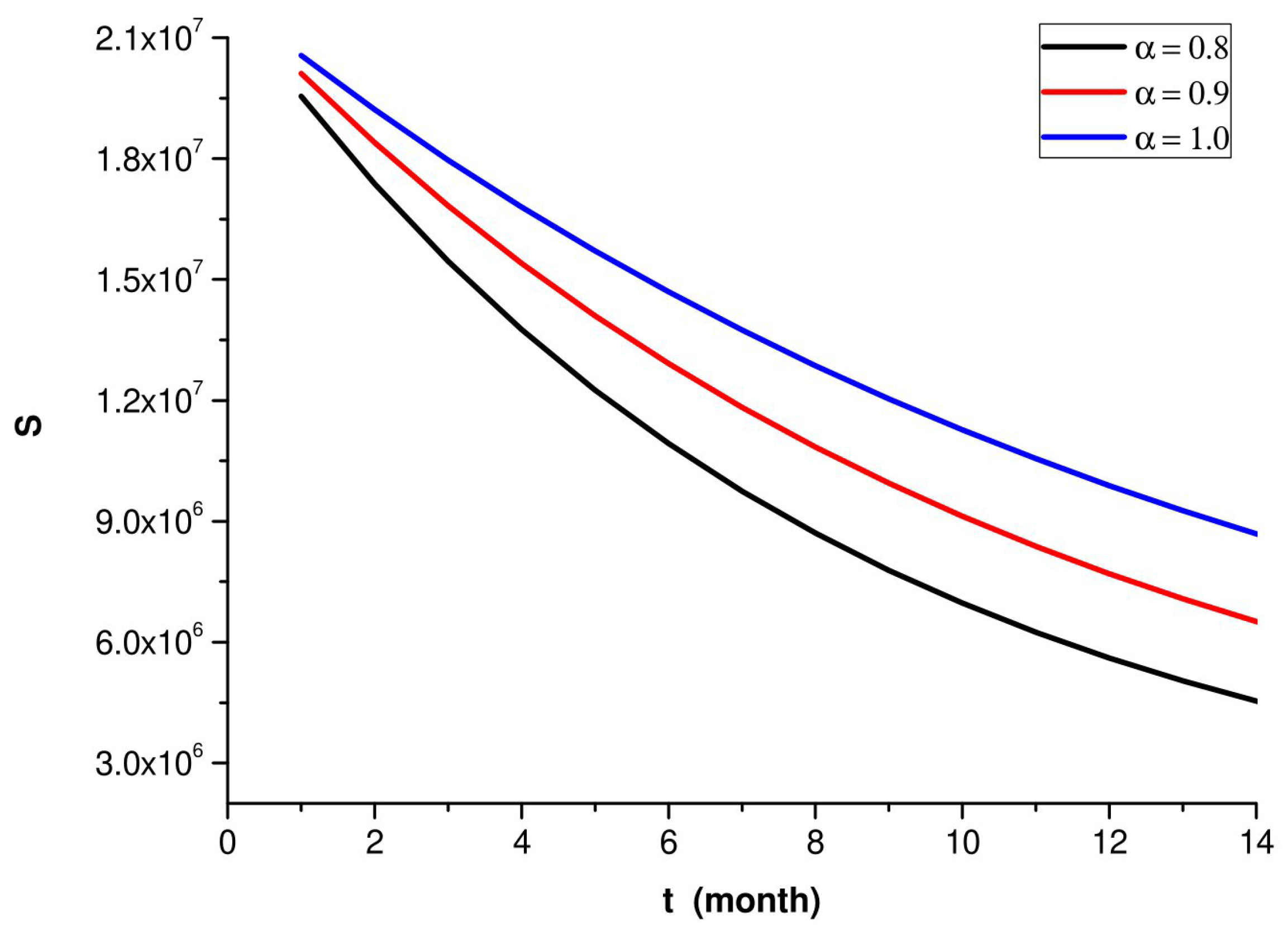
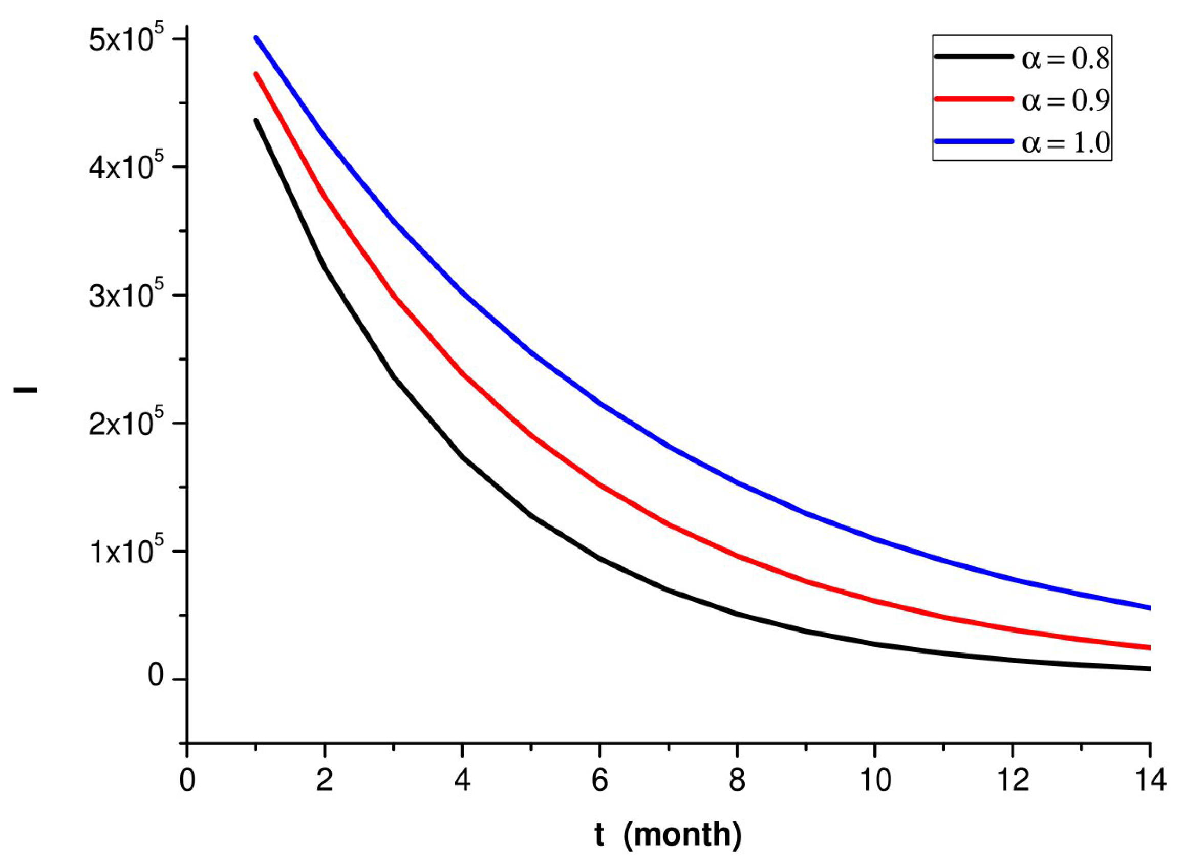
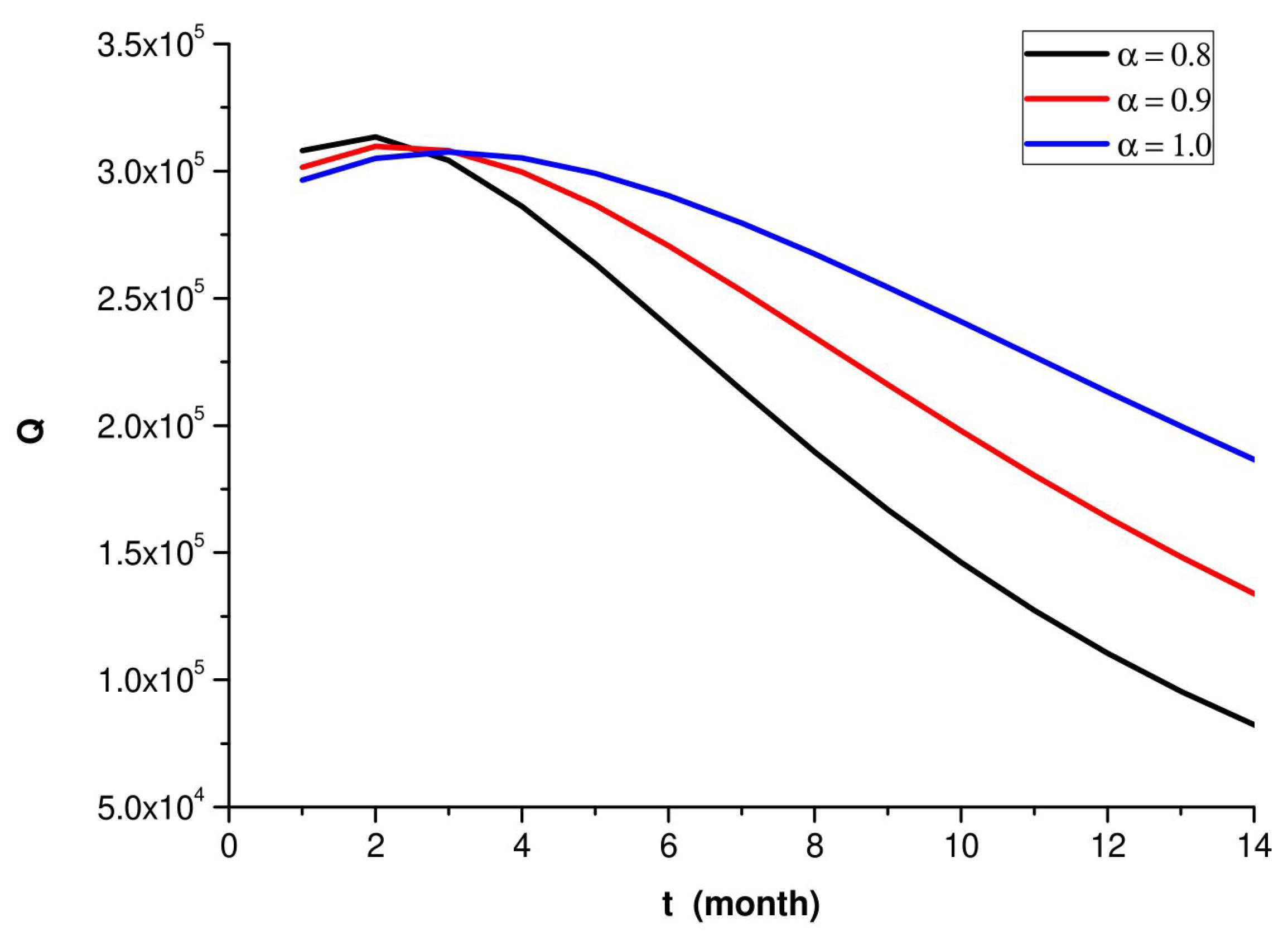
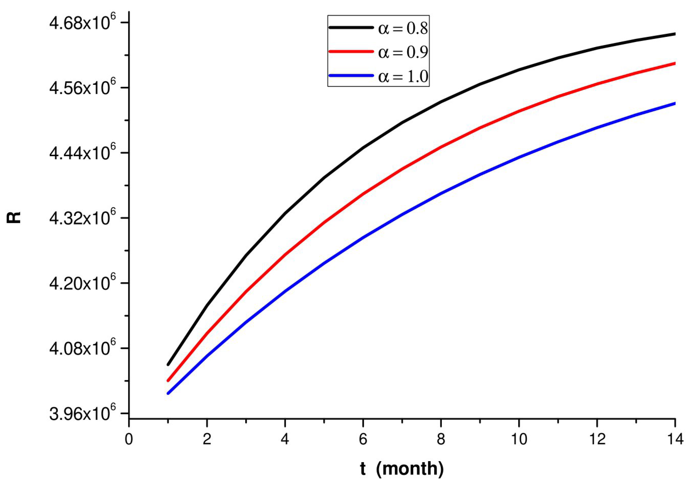
In the above figures, we can observe the following:

*

increase susceptible individuals decrease over time, and this number steadily progresses.

*

The number of infected individuals rapidly decreases and approaches zero.

*

The maximum value of individuals in quarantine at a certain time t decreases over time after implementation.

*

The number of recovered individuals rapidly increases over time.

*

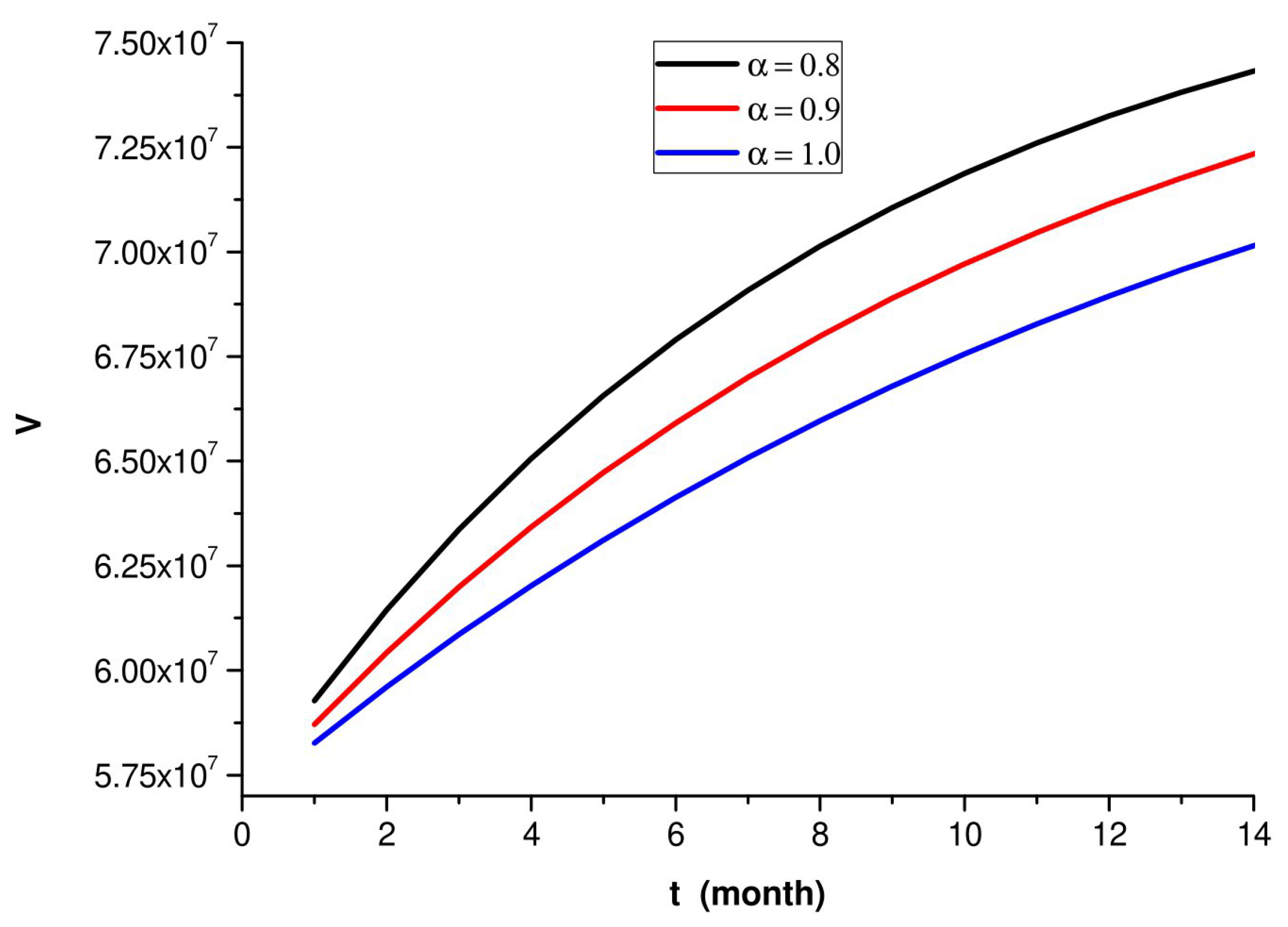
The number of vaccinated individuals rapidly increases over time.

4. Conclusions

In this study, the natural mortality rates in Türkiye were considered when applying a new fractional SIQRV model for COVID-19, and graphs were created using the numerical values. We investigated how the pandemic evolved with vaccination, taking into account the vaccination rate and the rate at which the vaccine begins to lose its protective effects. The basic reproduction rate, $R_0$, which is important for stability analysis, was determined by finding the fractional SIQRV model’s disease-free equilibrium point. The obtained values decreased steadily over time for the number of infected and susceptible people and rapidly approached zero, which represents the maximum number of people in quarantine at a given time.

The results of a mathematical model may not be exactly show when a pandemic will end or how the process will continue. Mathematical models mostly reveal the effect of the parameters used in the model on the pandemic in cases where the strategy for fighting pandemics does not change (where an extraordinary event, such as the discovery of a new drug, has not occurred).

From Figure 1, Figure 2, Figure 3, Figure 4 and Figure 5, we see that in the susceptibility increased with increasing different fractional orders. As a result, the infected class reduced, and so the implementation of quarantine continued this decrease. The recovery rate was also rapid because the number of people who became vaccinated and recovered from from disease also increased.

According to the official data of the Ministry of Health of the Republic of Türkiye, the number of COVID-19 cases was 31,054 in April 2023. This number only represents the number of officially confirmed cases, and it is clear that the actual number was higher (due to individuals who did not report to health institutions). As a result, the numerical results of the model and the actual data are in good agreement with the actual data. In addition, the results were more consistent as the $\alpha$ value (i.e., memory index) decreased. These results verify the applicability of the model and the ability to make accurate assessments for future time periods. Despite this, depending on the current developments related to the COVID-19 pandemic, this model is open to improvements.

References

- Bozkurt, F.; Yousef, A.; Abdeljawad, T. Analysis of the outbreak of the novel coronavirus COVID-19 dynamic model with control mechanisms. Results Phys. 2020, 19, 103586. [Google Scholar] [CrossRef] [PubMed]
- Brauer, F.; Castillo-Chavez, C.; Feng, Z. Mathematical Models in Epidemiology; Springer: New York, NY, USA, 2019; Volume 32. [Google Scholar]
- Allen, L.J.S. An Introduction to Mathematical Biology; Department of Mathematics and Statistics, Texas Tech University: Lubbock, TX, USA; Pearson Education: New York, NY, USA, 2007; 348p. [Google Scholar]
- Akram, T.; Abbas, M.; Ali, A. A numerical study on time fractional Fisher equation using an extended cubic B-spline approximation. J. Math. Comput. Sci. 2021, 22, 85–96. [Google Scholar] [CrossRef]
- Jassim, H.K.; Hussain, M.A.S. On approximate solutions for fractional system of differential equations with Caputo-Fabrizio fractional operator. J. Math. Comput. Sci. 2021, 23, 58–66. [Google Scholar] [CrossRef]
- Salama, F.M.; Ali, N.H.; Abd Hamid, N.N. Fast O(N) hybrid Laplace transform-finite difference method in solving 2D time fractional diffusion equation. J. Math. Comput. Sci. 2021, 23, 110–123. [Google Scholar] [CrossRef]
- Cao, Y.; Nikan, O.; Avazzadeh, Z. A localized meshless technique for solving 2D nonlinear integro-differential equation with multi-term kernels. Appl. Numer. Math. 2023, 183, 140–156. [Google Scholar] [CrossRef]
- Erdinç, Ü.; Bilgil, H.; Öztürk, Z. A Novel Fractional Forecasting Model for Time Dependent Real World Cases. REVSTAT-Stat. J. 2022. Available online: https://revstat.ine.pt/index.php/REVSTAT/article/view/468 (accessed on 1 May 2023).
- Öztürk, Z.; Bilgil, H.; Erdinç, Ü. An optimized continuous fractional grey model for forecasting of the time dependent real world cases. Hacet. J. Math. Stat. 2022, 51, 308–326. [Google Scholar] [CrossRef]
- Bozkurt, F.; Yousef, A.; Bilgil, H.; Baleanu, D. A mathematical model with piecewise constant arguments of colorectal cancer with chemo-immunotherapy. Chaos Solitons Fractals 2023, 168, 113207. [Google Scholar] [CrossRef]
- Podlubny, I. Fractional Differential Equations; Academy Press: San Diego, CA, USA, 1999. [Google Scholar]
- Van den Driessche, P.; Watmough, J. Reproduction numbers and sub-threshold endemic equilibria for compartmental models of disease transmission. Math. Biosci. 2002, 180, 29–48. [Google Scholar] [CrossRef]
- Turan, C.; Hacımustafaoğlu, M. Enfeksiyon Hastalıklarında ±R0 Oranı ve Klinik Anlamı Nedir? Çocuk Enfeksiyon Derg. 2020, 14, 55–56. [Google Scholar] [CrossRef]
- Allen, L.J.S. An Introduction to Mathematical Biology; Pearson Education Ltd.: New York, NY, USA, 2007; pp. 123–127. [Google Scholar]
- Bailey, N.T. The Mathematical Theory of Infectious Diseases and Its Applications, 2nd ed.; Charles Griffin and Company Ltd.: High Wycombe, UK, 1975. [Google Scholar]
- Hethcote, H.; Zhien, M.; Shengbing, L. Effects of quarantine in six endemic models for infectious diseases. Math. Biosci. 2002, 180, 141160. [Google Scholar] [CrossRef]
- Wang, S.; Ding, Y.; Lu, H.; Gong, S. Stability and bifurcation analysis of SIQR for the COVID-19 epidemic model with time delay. Math. Biosci. Eng. 2021, 18, 5505–5524. [Google Scholar] [CrossRef]
- Öztürk, Z.; Bilgil, H.; Sorgun, S. Stability Analysis of Fractional PSQp Smoking Model and Application in Turkey. New Trends Math. Sci. 2022, 10, 54–62. [Google Scholar] [CrossRef]
- Peter, O.J.; Shaikh, A.S.; Ibrahim, M.O.; Nisar, K.S.; Baleanu, D.; Khan, I.; Abioye, A.I. Analysis and dynamics of fractional order mathematical model of COVID-19 in Nigeria using atangana-baleanu operator. Comput. Mater. Contin. 2021, 66, 1823–1848. [Google Scholar] [CrossRef]
- Öztürk, Z.; Sorgun, S.; Bilgil, H.; Erdinç, Ü. New Exact Solutions of Conformable Time-Fractional Bad and Good Modified Boussinesq Equations. J. New Theory 2021, 37, 8–25. [Google Scholar] [CrossRef]
- Sun, C.; Yang, W. Global results for an SIRS model with vaccination and isolation. Nonlinear Anal. Real World Appl. 2010, 11, 4223–4237. [Google Scholar] [CrossRef]
- Öztürk, Z.; Sorgun, S.; Bilgil, H. SIQRV Modeli ve Nümerik Uygulaması. Avrupa Bilim Teknol. Derg. 2021, 28, 573–578. [Google Scholar] [CrossRef]
- Odagaki, T. Exact properties of SIQR model for COVID-19. Phys. A Stat. Mech. Appl. 2021, 564, 125564. [Google Scholar] [CrossRef]
- Kermack, W.O.; McKendrick, A.G. A contribution to the mathematical theory of epidemics. Proc. R. Soc. Lond. Ser. A Contain. Pap. Math. Phys. Character 1927, 115, 700–721. [Google Scholar]
- Yaro, D.; Omari-Sasu, S.K.; Harvim, P.; Saviour, A.W.; Obeng, B.A. Generalized Euler method for modeling measles with fractional differ ential equations. Int. J. Innov. Res. Dev. 2015, 4, 358–366. [Google Scholar]
- Bozkurt, F.; Yousef, A.; Abdeljawad, T.; Kalinli, A.; Al Mdallal, Q. A fractional-order model of COVID-19 considering the fear effect of the media and social networks on the community. Chaos Solitons Fractals 2021, 152, 111403. [Google Scholar] [CrossRef] [PubMed]
- Boyce, W.E.; DiPrima, R.C.; Meade, D.B. Elementary Differential Equations and Boundary Value Problems; John Wiley & Sons: Hoboken, NJ, USA, 2021. [Google Scholar]
- Bilgil, H.; Yousef, A.; Erciyes, A.; Erdinç, Ü.; Öztürk, Z. A fractional-order mathematical model based on vaccinated and infected compartments of SARS-CoV-2 with a real case study during the last stages of the epidemiological event. J. Comput. Appl. Math. 2023, 425, 115015. [Google Scholar] [CrossRef] [PubMed]