Article

Study on Structural Properties of Brain Networks Based on Independent Set Indices

by
Anagha Puthanpurakkal
and
Selvakumar Ramachandran
*
Department of Mathematics, Vellore Institute of Technology, Vellore 632014, India
*
Author to whom correspondence should be addressed.
Symmetry 2023, 15(5), 1032; https://doi.org/10.3390/sym15051032
Submission received: 9 February 2023 / Revised: 14 March 2023 / Accepted: 21 March 2023 / Published: 6 May 2023
(This article belongs to the Special Issue Topological Indices and Symmetry in Complex Networks)

Abstract

:
Studies of brain network organisation have swiftly adopted graph theory-based quantitative analysis of complicated networks. Small-world topology, densely connected hubs, and modularity characterise the brain’s structural and functional systems. Many measures quantify graph topology. It has not yet been determined which measurements are most appropriate for brain network analysis. This work introduces a new parameter applicable to brain network analysis. This parameter may help in the identification of symmetry and the study of symmetry breakdown in the brain. This is important because decreased symmetry in the brain is associated with a decreased chance of developing neurodevelopmental and psychiatric disorders. This work is to study brain networks using maximal independent set-based topological indices. These indices seem to depict significant properties of brain networks, such as clustering, small-worldness, etc. One new parameter introduced in this paper for brain network analysis depends on Zagreb topological indices and independence degree. This parameter is useful for analyzing clusters, rich clubs, small-worldness, and connectivity in modules.

1. Introduction

Graph theory is a branch of mathematics that deals with networks made up of points (vertices) connected by lines (edges). In light of graph theory, brain networks are composed of vertices and edges, where vertices represent neurons or brain regions, and edges represent the physical or functional connections between vertices.
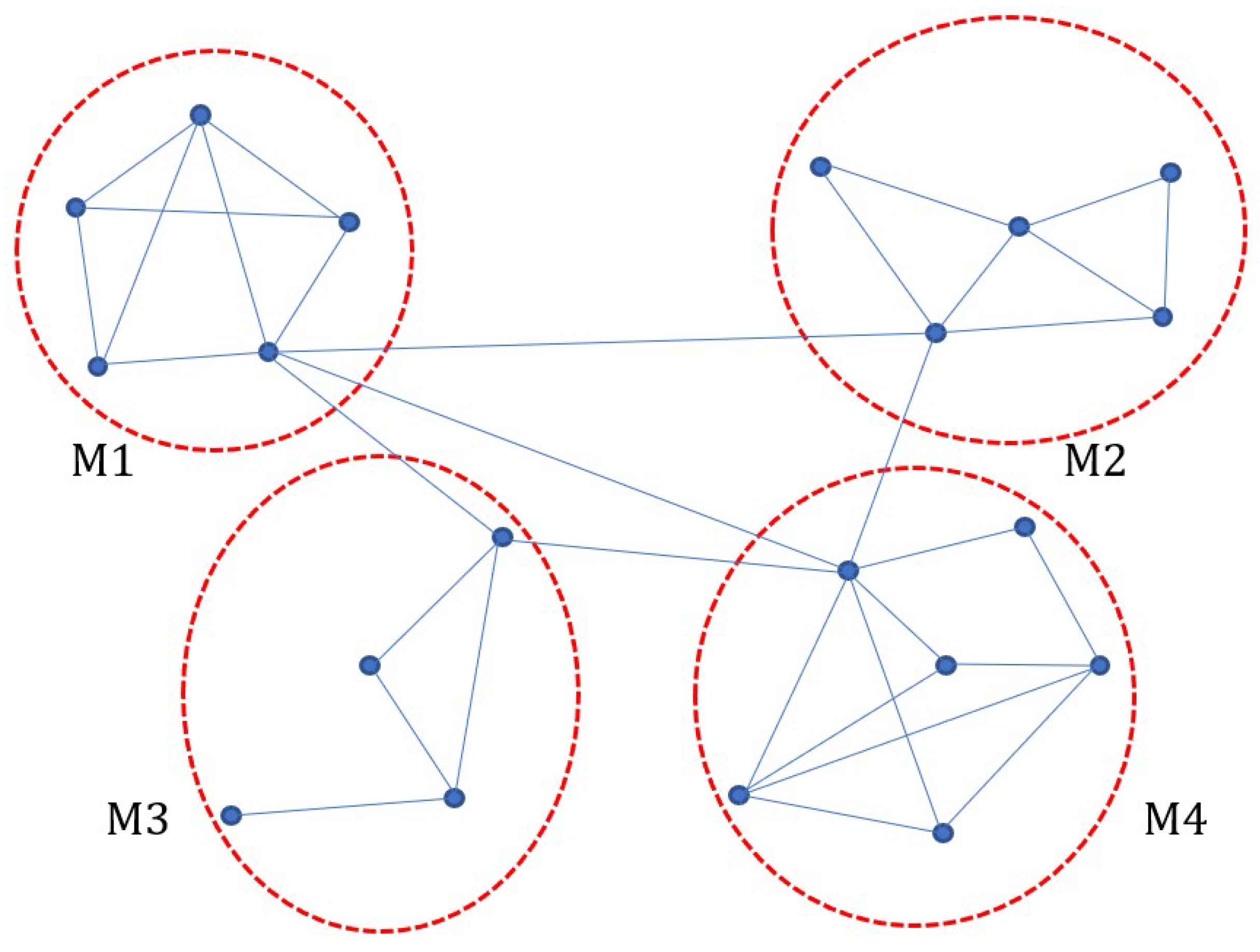
A brain network can be grouped into different communities or modules. A module is a collection of nodes with intense interconnectivity within clusters but sparse (incomplete) interconnectivity between clusters. A cluster is made up of a collection of nodes with connected neighbours [1,2,3]. Let G i be the subgraph of G that is induced by the neighbours of each vertex i, and let G i be the subgraph of G that is induced by both vertex i and its neighbours. The clustering coefficient was defined by Watts and Strogatz to be C C ( G ) = 1 / n i | E ( G i ) | / V ( G i ) 2 where | V ( G i ) | is the size of the vertex set of the graph G i , and | E ( G i ) | is the size of the edge set of the graph G i [4].
Some nodes within modules are referred to as provincial hubs if they are significant within their module but not necessarily for the overall network (local hubs). Some nodes, however, play a vital role in the transmission of information from one module to another, despite their lesser relevance within their own module. These nodes are known as connector hubs [5].
A node is determined to be a hub based on the following criteria: (1) degree and strength (local), (2) global centrality (betweenness or closeness), (3) community structure participation, and (4) vulnerability. Hubs and rich clubs serve crucial roles in global communication by facilitating the integration of information across multiple brain systems and providing the shortest, most efficient channels [6].
The hubs that are tied together form rich clubs. In other words, it uses a very small fraction of the brain’s volume and wire material to transport information very quickly (nodes). Rich clubs allow you to connect many modules or find the shortest path inside a module. Hence, damage to the rich club has a greater impact on the entire brain network than damage to any other area. Rich club hub connections are topologically short but physically lengthy, with only one or two intermediate nodes connecting any two nodes together. Rich clubs’ primary advantage is that they enable quicker and less obtrusive transmission between neurons.
Independent sets are an important topic in graph theory. An independent set I of a graph G is a set of vertices that consists of non-adjacent vertices of G. A maximal independent set is an independent set that is not a subset of any other independent set. Let G = ( V , E ) be a graph. A complement G ¯ of a graph G is a graph with the same set of vertices V and an edge between a pair if and only if there is no edge between them in G [7]. There is work that has gained a lot of attention connecting independent numbers and topological indices [8].
The topological indices of a graph are numbers that represent structural information about the graph. Topological indices have received much attention and acceptance in the fields of chemical graph theory, molecular topology, and mathematical chemistry. There are a lot of topological indices based on degree, distance, eccentricity, etc. Numerous chemical indices, such as Zagreb indices, Wiener index, etc., are invented in theoretical chemistry and compute many degree-based topological indices of some derived networks, which have valuable applications in drug storage and system administration [9].
The Wiener index W ( G ) is an old index and the first topological index used in chemistry [10]. It is a distance-based topological index introduced in 1947 by Chemist Wiener. It is defined as the sum of distances between all the vertices of G; for further information, see [11]. Among all topological indices, degree-based topological indices have the greatest significance. A large number of degree-based graph invariants are studied in both the mathematical and chemistry literature [12,13,14], but among them, Zagreb indices are widely used. The Zagreb indices, M 1 ( G ) and M 2 ( G ) were introduced more than forty years ago [15,16] and are based on vertex degree. They are defined as, M 1 ( G ) = v V ( G ) d 2 ( v ) = u v E ( G ) [ d ( u ) + d ( v ) ] , M 2 ( G ) = u v E ( G ) d ( u ) d ( v ) , where d ( v ) is the degree of the vertex v in G. More information on Zagreb indices is provided in [17,18], and Zagreb co-indices are defined in [19] as M ¯ 1 ( G ) = [ d ( u ) + d ( v ) ] and M ¯ 2 ( G ) = d ( u ) d ( v ) , where u v is not an edge in E ( G ) .
Random networks evolved from the Erdős–Rényi model have the property of a minimum average path length between every pair of nodes. This property is called small-worldness. This concept is popularized by terms such as “six degrees of separation” between any two individuals. Social networks, brain networks, the connectivity of the Internet, and gene networks all exhibit small-world network characteristics [20].
Recent extensive neuroimaging studies suggest anatomical differences between the left and right hemispheres of the human brain in most regions. Several studies have found evidence of hemispheric structural asymmetry in both cortical and subcortical areas. It is interesting to note that various neurodevelopmental and psychiatric illnesses have been associated with altered functional hemisphere asymmetries [21]. In this light, the fact that many neurodevelopmental and psychiatric disorders have been associated with reduced brain asymmetries—such as increased brain symmetry—is very intriguing [21,22]. Complex biological structures, such as the brain, may not always benefit from symmetry since it would lead to difficulties with multitasking, excessive energy use, and bilateral action control. Since all brain systems must eventually evolve, the breakdown of symmetry is a crucial step.
Dementia is a level of cognitive decline that affects a person’s ability to think, remember, and reason in everyday activities. It is a symptom of Alzheimer’s disease. Some people with dementia lose their control over emotions, and it leads to a personality change in that individual. The diagnosis of this starts with the progressive decline in memory, where memory is connected with connections in the brain network. Therefore, connections are of much importance in the diagnosis and treatment of dementia.
The primary objective of this study is to offer new topological indices for brain network analysis that are based on the maximal independent set. Since the strength of these indices depends on the connections between the vertices inside each module, it is intended that they be built in a way that allows one to learn about each module and how strong it is. This study offers a new parameter based on the total number of maximum independent sets T ( G ) and the new independent topological index I M 1 ( G ) . The connectedness of this new parameter, I M 1 ( G ) / T ( G ) , is inversely correlated, and 1 I M 1 ( G ) / T ( G ) n T ( G ) . If the parameter value is close to its lower bound, this implies that the module is strongly related.
This study also introduces a brand-new parameter, ρ , where ρ = c o n n e c t e d n e s s [ I M 1 ( G ) / T ( G ) ] . A module is strong in terms of connectivity if its value is higher than zero. This parameter can be useful in the research of brain disease and brain analysis since the loss of connections between vertices is a common cause of brain diseases, such as Alzheimer’s.
Topological indices are mainly used in chemical graph theory. This work can help researchers recognize the importance of topological indices for brain network analysis. Since it is currently unknown which measurements are optimal for brain network analysis, parameter studies are pertinent. This paper, therefore, sheds light on the fact that topological indices can be effectively used on network structure rather than chemical structure. Further, it is a simple, non-invasive, and cost-effective procedure. Topological indices are invariant with respect to isomorphism. Therefore, the capturing of images will not affect the detection of dementia much.
In this paper, the independence of each vertex of a graph and its basic properties are defined in the first section. In the second section, independent Zagreb topological indices are introduced, and the indices of some families of small-world graphs are calculated. The third section discusses the join and corona products of graphs, and the final section contains the results and discusses their application.

2. Independence Degree of a Vertex

In this chapter, the independence degree of the vertex, v, is defined, and the basic properties of this degree are studied.
 Definition 1.
Let G be a connected graph and v G . The number of maximal independent sets of G containing v is called the independence degree of v. It is denoted as d I ( v ) .
 Observation 1.
1 d I ( v ) T ( G ) , where T ( G ) is the total number of maximal independent sets.
 Proposition 1.
Let G be a star graph S n with n + 1 vertices, then d I G ¯ ( v ) = d G ( v ) and T ( G ¯ ) = n .
 Proof.
Since G S n , G ¯ is a disconnected graph with a complete graph K n and an isolated vertex. Therefore, T ( G ¯ ) = n . Further, every vertex in K n has d I ( v ) = 1 , and an isolated vertex has d I ( v ) = n . □
 Corollary 1.
If G K , then d I G ( v ) = d I G ¯ ( v ) and T ( G ¯ ) = 1 .
 Observation 2.
Let I 1 , I 2 , I 3 , , I m be the maximal independent sets of G, then m γ ( G ) v V ( G ) m Γ ( G ) , where γ ( G ) , Γ ( G ) is the minimum and maximum cardinality of maximal independent sets of G, respectively.
 Observation 3.
Let G = i = 1 m G i be the disjoint union of graphs G 1 , G 2 , , G m . Then T ( G ) = i = 1 m T ( G i ) and for v V ( G i ) , d I G ( v ) = d I G i ( v ) j = 1 m T ( G j ) , j i .
 Proposition 2.
Let G S r , s (double star graph) with r + s + 2 vertices then T ( G ) = 3 and
d I ( v ) = 1 ; i f v i s c e n t r e v e r t e x 2 ; i f v i s p e n d a n t v e r t e x .
 Proof.
Let { v , v 1 , v 2 , , v r , w , w 1 , w 2 , , w s } V ( G ) with centre vertices { v , w } . There are three maximal independent sets; { v 1 , v 2 , , v r , w 1 , w 2 , , w s } , { v , w 1 , w 2 , , w s } , { w , v 1 , v 2 , , v r } . Hence T ( G ) = 3 . Hence
d I ( v ) = 1 ; if v is centre vertex 2 ; if v is pendant vertex

3. Independent Indices of a Graph

A network is an arrangement of elements made for the systematic sharing of information. The small-world property is a property of networks in which short communication paths can be found between vertices. Most of the complex networks have a small-world topology. It is an attractive model for the organisation of brain structural and functional networks because a small-world topology can support both disaggregated and integrated information processing. Further, small-world networks are cost-effective, trying to reduce wiring costs while supporting high dynamic complexity. Therefore, this section defines independent indices and discusses independent indices for some families of graphs with the small-world property.
 Definition 2.
The first independent, second independent, and modified first Zagreb indices of a simple connected graph G are defined as,
I M 1 ( G ) = v V ( G ) d I 2 ( v )
I M 2 ( G ) = u v E ( G ) d I ( u ) d I ( v )
I M 1 * ( G ) = u v E ( G ) [ d I ( u ) + d I ( v ) ] .
 Lemma 1.
Let S r be the star graph with r + 1 vertices and K n be the complete graph with n vertices, then T ( S r ) = 2 and T ( K n ) = n and d I ( v ) = 1 v V ( S r ) or v V ( K n ) .
 Proposition 3.
  • For S q with q + 1 vertices, I M 1 ( S q ) = q + 1 , I M 2 ( S q ) = q and I M 1 * ( S q ) = 2 q .
  • For K n , I M 1 ( K n ) = n , I M 2 ( K n ) = n ( n 1 ) / 2 and I M 1 * ( K n ) = n ( n 1 ) .
  • For a double star graph S p , q with p + q + 2 vertices, I M 1 ( S p , q ) = 4 ( p + q ) + 2 , I M 2 ( S p , q ) = 2 ( p + q ) + 1 and I M 1 * ( S p , q ) = 3 ( p + q ) + 2 .
 Definition 3
([23]). Domination degree d d ( v ) is the number of minimal dominating sets (MDs) of a graph G that contains a vertex v; v V ( G ) . T m ( G ) is the total number of MDs in G. The first domination D M 1 ( G ) , second domination D M 2 ( G ) , and modified first Zagreb indices D M 1 * ( G ) of the graph are v V ( G ) d d 2 ( v ) , u v E ( G ) d d ( u ) × d d ( v ) , u v E ( G ) [ d d ( u ) + d d ( v ) ] , respectively.
 Proposition 4.
Let G be S r , s and D M 1 , D M 2 , D M 1 * are the first domination, second domination, and modified first Zagreb indices of G, respectively. Then, I M 1 ( S r , s ) = D M 1 ( S r , s ) 6 , I M 2 ( S r , s ) = ( D M 2 ( S r , s ) 2 ) / 2 , I M 1 * ( S r , s ) = ( 3 D M 1 * ( S r , s ) 4 ) / 4 .
 Proof.
From [23], D M 1 ( G ) = 4 ( r + s + 2 ) , D M 2 ( G ) = 4 ( r + s + 1 ) , and D M 1 * ( G ) = 4 ( r + s + 1 ) . Therefore, by substitution of these values, the results are obtained. □
 Lemma 2.
Let G K r , s , then T ( G ) = 2 and d I ( v ) = 1 v V ( G ) and T m ( G ) T m ( G ¯ ) = T ( G ) ; T m ( G ) is the total number of MDs.
 Proof.
Let { u 1 , u 2 , , u r , v 1 , v 2 , , v s } be the set of all vertices of G, then there are two maximal independent sets in G. They are { u 1 , u 2 , , u r } , { v 1 , v 2 , , v s } . Therefore, d I ( v ) = 1 , since these sets are disjointed. However, T m ( G ) = r s + 2 and
d d ( v ) = r + 1 ; if v { v 1 , v 2 , , v s } s + 1 ; if v { u 1 , u 2 , , u r } .
Further, G ¯ is a disconnected graph with K r and K s as its components. Therefore, T m ( G ¯ ) = r s . Therefore, T m ( G ) T m ( G ¯ ) = r s + 2 r s = 2 = T ( G ) . □
 Theorem 1.
If G K r , s , then I M 1 ( G ) = r + s , I M 2 ( G ) = r s , I M 1 * ( G ) = 2 r s .
 Proof.
Using the definitions and Lemma 4, the result is obtained. □
 Corollary 2.
Let G K r , s then I M 1 ( G ¯ ) = M 1 ( G ) = D M 1 ( G ¯ ) = s r × I M 1 ( G ) ,
I M 2 ( G ¯ ) = D M 2 ( G ¯ ) = M 2 ( G ) ( M 1 ( G ) ) / 2 = M ¯ 2 ( G ) ,
I M 1 * ( G ¯ ) = I M 1 ( G ¯ ) I M 1 * ( G ) ,
I M 1 * ( G ) = 2 M 1 ( G ) / I M 1 ( G ) = D M 1 * ( G ) M 1 ( G ) .
 Proof.
I M 1 ( G ¯ ) = s r ( r + s ) = r s × I M 1 ( G )
(By Theorem 1).
M 1 ( G ) = r s 2 + s r 2 = r s ( s + r ) = I M 1 ( G ¯ ) .
I M 1 ( G ¯ ) = D M 1 ( G ¯ ) ( s i n c e d I G ¯ ( v ) = d d G ¯ ( v ) ) .
Since G ¯ is a disconnected graph with K r and K s as its components,
I M 2 ( G ¯ ) = r ( r 1 ) / 2 s 2 + s ( s 1 ) / 2 r 2 = r s ( ( r s ) s / 2 + ( s 1 ) r / 2 ) = r s ( 2 r s ( r + s ) ) / 2 = r 2 s 2 r s ( r + s ) / 2 = M 2 ( G ) ( M 1 ( G ) ) / 2
I M 1 * ( G ¯ ) = r ( r 1 ) / 2 × 2 s + s ( s 1 ) / 2 × 2 r = r s ( r + s 2 ) = r s ( r + s ) 2 r s = I M 1 ( G ¯ ) I M 1 * ( G ) .
2 M 1 ( G ) / I M 1 ( G ) = 2 r s ( r + s ) / ( r + s ) = 2 r s = I M 1 * ( G ) .
D M 1 * ( G ) = r s ( r + s + 2 ) = r s ( r + s ) + 2 r s = M 1 ( G ) + I M 1 * ( G ) . □
 Definition 4.
An undirected graph called the windmill graph W p q is created for the p ( > 2 ) and q ( > 2 ) by combining q copies of the complete graph K p at a common universal vertex.
 Lemma 3.
Let G W p q (Windmill graph) then T ( G ) = ( p 1 ) q + 1 and
d I ( v ) = 1 ; i f v i s t h e c e n t r e v e r t e x ( p 1 ) q 1 ; o . w .
 Proof.
Two types of the maximal independent sets are only possible for the Windmill graph. The first type is the set that contains only the centre. The second type is one vertex from each complete graph K p 1 (the complete graph that exists in W p q after its centre vertex is removed) that is contained in W p q . There are ( p 1 ) q maximal independent sets of type 2. □
 Theorem 2.
If G W p q then
I M 1 ( G ) = 1 + q ( p 1 ) 2 q 1
I M 2 ( G ) = q ( ( p q ) q + ( p 1 ) 2 q 1 ( p 2 ) / 2 )
I M 1 * ( G ) = q ( p 1 ) ( 1 + ( p 1 ) q )
 Proof.
I M 1 ( G ) = v V ( G ) d I 2 ( v ) = 1 × 1 2 + ( p 1 ) q ( ( p 1 ) q 1 ) 2 = 1 + q ( p 1 ) 2 q 1
There are two types of edges in G. The first type E 1 is the collection of all edges that intersect with the centre vertex, and the second type E 2 is the set of all edges of the complete graph K p 1 ,
I M 2 ( G ) = u v E 1 ( 1 × ( p 1 ) q 1 ) + u v E 2 ( ( p 1 ) q 1 × ( p 1 ) q 1 ) = q ( p 1 ) ( 1 × ( p 1 ) q 1 ) + q ( p 1 ) ( p 2 ) / 2 ( ( p 1 ) q 1 ) 2 = q ( p 1 ) q + ( q ( p 2 ) ( p 1 ) 2 q 1 ) / 2 = q ( ( p q ) q + ( p 1 ) 2 q 1 ( p 2 ) / 2 )
I M 1 * ( G ) = u v E 1 ( 1 + ( p 1 ) q 1 ) + u v E 2 ( ( p 1 ) q 1 + ( p 1 ) q 1 ) = q ( p 1 ) ( 1 + ( p 1 ) q 1 ) + q ( p 1 ) ( p 2 ) / 2 × 2 ( p 1 ) q 1 = q ( p 1 ) + q ( p 1 ) q + q ( p 1 ) q ( p 2 ) = q ( p 1 ) [ 1 + ( p 1 ) q 1 ( 1 + p 2 ) ] = q ( p 1 ) ( 1 + ( p 1 ) q )
 Definition 5
([24]). Let G 1 and G 2 be any two graphs, and the Cartesian product G 1 × G 2 is defined as the graph has vertex set V ( G 1 ) × V ( G 2 ) such that any two vertices u = ( u 1 , u 2 ) and v = ( v 1 , v 2 ) are adjacent if and only if either u 1 = v 1 and u 2 , v 2 E ( G 2 ) or u 2 = v 2 and u 1 , v 1 E ( G 1 ) .
  • Book graph B r is S r × P 2 , where S r is the star graph with r + 1 vertices.
 Lemma 4.
If G B r then T ( G ) = 2 r and d I ( v ) = 1 ; i f v i s t h e c e n t r e 2 r 1 ; o . w
 Proof.
Let u v be the centre edge, and u , v be the set of centre vertices in the book graph. Let { v 1 , v 2 , , v r } be the collection of neighbours of centre vertex v. Similarly, { u 1 , u 2 , , u r } is the collection of neighbours of centre vertex u. There are two different kinds of maximal independent sets. The first type is { v , u 1 , u 2 , , u r } and { u , v 1 , v 2 , , v r } . Only those maximal independent sets other than u and v that are created by selecting one vertex from each section fall under the second type. Therefore, there exist 2 r 2 maximal independent sets of the second type. Thus T ( G ) = 2 r and d I ( v ) = 1 ; if v is the centre 2 r 1 ; otherwise , for all v V ( B r )
 Theorem 3.
For G B r where r 3 ,
I M 1 ( G ) = r 2 2 r 1 + 2 .
I M 2 ( G ) = r 2 2 r [ 1 / 4 + 1 / 2 r ] + 1 .
I M 1 * ( G ) = 2 r ( 2 r + 1 ) + 2 .
 Proof.
I M 1 ( G ) = 2 r × ( 2 r 1 ) 2 + 2 × 1 2 = r 2 2 r 1 + 2
There are three types of edges E 1 , E 2 , and E 3 in B r . Consider E 1 to be the set of r edges whose end vertices have the same independence degree 2 r 1 , E 2 to be the edge set that contains only the edge u v whose end vertices have the same independence degree 1, and E 3 to be the set of 2 r edges with one vertex of independent degree 1 and the other vertex of independence degree 2 r 1 . Hence,
I M 2 ( G ) = u v E 1 ( 2 r 1 ) 2 + u v E 2 1 2 + u v E 3 1 ( 2 r 1 ) . = r 2 2 r 2 + 1 + 2 r 2 r 1 = r 2 2 r 2 + r 2 r + 1 = r 2 2 r [ 1 / 4 + 1 / 2 r ] + 1
I M 1 * ( G ) = u v E 1 ( 2 r 1 + 2 r 1 ) + u v E 2 ( 1 + 1 ) + u v E 3 ( 1 + 2 r 1 ) = r 2 r + 2 + 2 r ( 1 + 2 r 1 ) = r 2 r + 2 + 2 r + r 2 r = r 2 r + 1 + 2 r + 2 = 2 r ( 2 r + 1 ) + 2
 Corollary 3.
I M 2 ( B r ) = [ D M 1 ( B r ) ( 2 r + 16 ) ] / 2 = 1 / 2 I M 1 ( B r ) + r 2 r
 Proof.
1 / 2 I M 1 ( B r ) + r 2 r = 1 / 2 [ r 2 2 r 1 + 2 ] + r 2 r = r 2 2 r 2 + r 2 r + 1 = r 2 2 r [ 1 / 4 + 1 / 2 r ] + 1 = I M 2 ( B r )
From [23],
[ D M 1 ( B r ) ( 2 r + 16 ) ] / 2 = [ 2 r ( 2 r 1 + 1 ) 2 + 18 ( 2 r + 16 ) ] / 2 = r ( 2 2 r 2 + 1 + 2 × 2 r 1 ) + 9 ( r + 8 ) = r 2 2 r 2 + r + r 2 r + 1 r = r 2 2 r 2 + r 2 r + 1 = I M 2 ( B r )
 Lemma 5.
Let G K n 1 , n 2 , , n k then T ( G ) = k and d I ( v ) = 1 v V ( G ) .
 Theorem 4.
If G K n 1 , n 2 , , n k then
I M 1 ( G ) = k
I M 2 ( G ) = i = 2 k n 1 n i + i = 3 k n 2 n i + + n k 1 n k .
I M 1 * ( G ) = 2 [ i = 2 k n 1 n i + i = 3 k n 2 n 1 + + n k 1 n k ]
 Proof.
The number of edges in G = i = 2 k n 1 n i + i = 3 k n 2 n i + + n k 1 n k and from the definition of the independence indices, the result is obtained. □
 Definition 6.
A graph consisting of r triangles, t pendant paths of length 2, and s pendant edges sharing a common vertex is known as a firefly graph, F r , s , t .
 Lemma 6.
Let G F r , s , t with r , s 0 and t 1 , then T ( G ) = 2 r + t + 1 and
d I ( v ) = 1 ; i f v i s t h e c e n t r e v e r t e x 2 r + t 1 ; i f v t r i a n g l e s o r m i d d l e p o i n t s o f p e n d a n t p a t h s 2 r + t ; i f v i s a p e n d a n t v e r t e x o f p e n d a n t e d g e s 2 r + t 1 + 1 ; i f v e n d p o i n t s o f p e n d a n t p a t h s , for any vertex v V ( G ) .
 Proof.
There are two types of maximal independent sets. The first type is the set containing the centre and all endpoints of pendant paths of length 2. The second type is the set containing all endpoints of pendant edges, one vertex (except the centre) of each triangle, and at most t middle points of pendant paths of length 2 (the absence of each middle point of pendant paths is replaced by the corresponding endpoints of pendant paths), and its cardinality is 2 r + t . □
 Theorem 5.
If G F r , s , t with r , s 0 and t 1 , then
I M 1 ( G ) = 1 + 2 2 r + 2 t 1 ( r + t + 2 s ) + t ( 1 + 2 r + t )
I M 2 ( G ) = 2 r + t ( r + t + s ) + 2 2 r + 2 t 2 ( r + t )
I M 1 * ( G ) = ( 1 + 2 r + t ) ( 2 r + s + t ) + t ( 1 + 2 r + t 1 )
 Proof.
Let G be a firefly graph F r , s , t with order 2 r + s + 2 t + 1 where r is the number of triangles, t is the number of pendant paths of length 2, and s is the number of pendant edges.
I M 1 ( G ) = 1 ( 1 2 ) + ( 2 r + t ) ( 2 r + t 1 ) 2 + t ( 2 r + t 1 + 1 ) 2 + s ( 2 r + t ) 2 = 1 + ( 2 r + t ) ( 2 2 t + 2 r 2 ) + t ( 2 2 t + 2 r 2 + 1 + 2 t + r ) + s ( 2 2 r + 2 t ) = 1 + r 2 2 t + 2 r 1 + t 2 2 t + 2 r 2 + t 2 2 t + 2 r 2 + t + t 2 t + r + s 2 2 r + 2 t = 1 + 2 2 r + 2 t 1 ( r + t + 2 s ) + t ( 1 + 2 r + t )
There are four types of edges E 1 , E 2 , E 3 , and E 4 in G. E 1 is the collection of edges containing edges between vertices (except the centre) of a triangle, and its cardinality is r; E 2 is the collection of edges whose one vertex is the centre, and the other vertex is the vertex of the triangle or the middle point of pendant paths of length 2, and its cardinality is ( 2 r + t ) ; E 3 is the set containing edges with one vertex being the centre and the other vertex is the pendant vertex, and its cardinality is s; and E 4 is the collection of edges whose one vertex is the middle point, and the other vertex is the endpoint of a pendant path of length 2, and its cardinality is t.
I M 2 ( G ) = u v E 1 ( 2 t + r 1 ) ( 2 t + r 1 ) + u v E 2 1 ( 2 r + t 1 ) + u v E 3 1 ( 2 r + t ) + u v E 4 2 r + t 1 ( 1 + 2 r + t 1 ) = r 2 2 r + 2 t 2 + ( 2 r + t ) 2 r + t 1 + s 2 r + t + t ( 2 r + t 1 + 2 2 r + 2 t 2 ) = r 2 2 r + 2 t 2 + r 2 r + t + t 2 r + t 1 + s 2 r + t + t 2 r + t 1 + t 2 2 r + 2 t 2 = 2 r + t ( r + t + s ) + 2 2 r + 2 t 2 ( r + t )
I M 1 * ( G ) = u v E 1 ( 2 r + t 1 + 2 r + t 1 ) + u v E 2 ( 1 + 2 r + t 1 ) + u v E 3 ( 1 + 2 r + t ) + u v E 4 ( 2 r + t 1 + ( 1 + 2 r + t 1 ) ) = r 2 r + t + ( 2 r + t ) ( 1 + 2 r + t 1 ) + s ( 1 + 2 r + t ) + t ( 1 + 2 r + t ) = r 2 r + t + 2 r + r 2 r + t + t + t 2 r + t 1 + s + s 2 r + t + t + t 2 r + t = 2 r + t ( 2 r + s + t ) + ( 2 r + t + s ) + t ( 1 + 2 r + t 1 ) = ( 1 + 2 r + t ) ( 2 r + s + t ) + t ( 1 + 2 r + t 1 )
 Corollary 4.
Let G be a stretched graph F 0 , s , t with s , t 1 then
I M 1 ( G ) = 1 + 2 2 t 1 ( t + 2 s ) + t ( 1 + 2 t ) I M 2 ( G ) = 2 t ( t + s ) + t 2 2 t 2 I M 1 * ( G ) = ( 1 + 2 t ) ( t + s ) + t ( 1 + 2 t 1 )
 Corollary 5.
Suppose G F r , 0 , t with r , t 1 . Then
I M 1 ( G ) = 1 + 2 2 r + 2 t 1 ( r + t ) + t ( 1 + 2 r + t )
I M 2 ( G ) = ( 2 r + t + 2 2 r + 2 t 2 ) ( r + t )
I M 1 * ( G ) = ( 1 + 2 r + t ) ( 2 r + t ) + t ( 1 + 2 r + t 1 )
 Lemma 7.
The total number of maximal independent sets in G F r , s , 0 with r , s 1 is T ( G ) = 1 + 2 r . For any vertex v V ( G ) , d I ( v ) = 1 ; i f v i s t h e c e n t r e v e r t e x 2 r ; i f v i s t h e p e n d a n t v e r t e x 2 r 1 ; i f v t r i a n g l e s
 Proof.
A set contains only a centre, and a set contains one vertex (other than the centre) from each triangle, and all pendent vertices are the two possible maximal independent sets. □
 Theorem 6.
If G F r , s , 0 with r 1 and s 1 , then
I M 1 ( G ) = 2 2 r 1 ( 2 s + r ) + 1
I M 2 ( G ) = r 2 2 r 2 + 2 r ( r + s )
I M 1 * ( G ) = ( 1 + 2 r ) ( 2 r + s )
 Proof.
I M 1 ( G ) = 1 ( 1 2 ) + s ( 2 r ) 2 + 2 r ( 2 r 1 ) 2 = 1 + s 2 2 r + r 2 2 r 1 = 2 2 r 1 ( 2 s + r ) + 1
There are three edge sets E 1 , E 2 , and E 3 , where E 1 is the set of edges whose both end vertices are vertices of triangles (other than the centre), E 2 is the collection of edges whose one vertex is the centre and the other vertex is a vertex of triangles, and E 3 is the collection of edges whose one vertex is the centre and the other vertex is a pendant vertex.
I M 2 ( G ) = E 1 ( 2 r 1 ) ( 2 r 1 ) + E 2 ( 1 ( 2 r 1 ) ) + E 3 1 ( 2 r ) = r ( 2 r 1 ) ( 2 r 1 ) + 2 r ( 1 ( 2 r 1 ) ) + s ( 1 ( 2 r ) ) = r 2 2 r 2 + r 2 r + s 2 r = r 2 2 r 2 + 2 r ( r + s )
I M 1 * ( G ) = E 1 ( 2 r 1 + 2 r 1 ) + E 2 ( 1 + 2 r 1 ) + E 3 ( 1 + 2 r ) = r ( 2 r 1 + 2 r 1 ) + 2 r ( 1 + 2 r 1 ) + s ( 1 + 2 r ) = r 2 r + 2 r + r 2 r + s + s 2 r = 2 r ( 2 r + s ) + ( 2 r + s ) = ( 1 + 2 r ) ( 2 r + s )
 Definition 7.
A planar, undirected graph with 2 n + 1 vertices and 3 n edges is the friendship graph F n . The n copies of the cycle graph C 3 can be joined at a common vertex to create the friendship graph F n , which has this vertex as its universal vertex.
 Corollary 6.
Let G F r , 0 , 0 be the friendship graph, then
I M 1 ( G ) = r 2 2 r 1 + 1
I M 2 ( G ) = r ( 2 2 r 2 + 2 r )
I M 1 * ( G ) = 2 r ( 1 + 2 r )
 Proposition 5.
If G F 0 , 0 , t , then
I M 1 ( G ) = 1 + t ( 2 2 t 1 )
I M 2 ( G ) = t ( 2 t 1 + 2 2 t 2 )
I M 1 * ( G ) = ( 1 + 2 t 1 + 2 t ) t .
 Proof.
If G F 0 , 0 , t , then T ( G ) = 2 t and d I ( v ) = 1 ; if v is the root 2 t 1 ; if v is the middle point or endpoint . Therefore, according to the definition of indices, the results are obtained. □

4. Graph Operations and Independent Indices

From given small communities, using graph operations, such as the join and corona products, a large community or whole brain network can be obtained, and vice versa.
  • A join of two graphs G 1 and G 2 is denoted by G 1 + G 2 and it is the graph on the vertex set V 1 V 2 and the edge set E 1 E 2 { u 1 u 2 ; u 1 V 1 , u 2 V 2 } , where G 1 and G 2 are graphs with disjoint vertex sets V 1 and V 2 [25].
 Lemma 8.
Let G 1 and G 2 be any graphs of n 1 and n 2 vertices, respectively. Then T ( G 1 + G 2 ) = T ( G 1 ) + T ( G 2 ) and d I G 1 + G 2 ( v ) = d I G 1 ( v ) ; i f v V ( G 1 ) d I G 2 ( v ) ; i f v V ( G 2 )
 Proof.
Only two types of maximal independent sets are in G 1 + G 2 . They are the maximal independent sets of G 1 and the maximal independent sets of G 2 . Hence the result. □
 Theorem 7.
Let G 1 and G 2 be any connected graphs with n 1 and n 2 vertices and m 1 and m 2 edges, respectively. Then
I M 1 ( G 1 + G 2 ) = I M 1 ( G 1 ) + I M 2 ( G 2 )
I M 2 ( G 1 + G 2 ) = I M 2 ( G 1 ) + I M 2 ( G 2 ) + σ ( G 1 ) σ ( G 2 )
I M 1 * ( G 1 + G 2 ) = I M 1 * ( G 1 ) + I M 1 * ( G 2 ) + n 2 σ ( G 1 ) + n 1 σ ( G 2 )
where σ ( G ) = v V ( G ) ) d I ( v ) .
 Proof.
I M 1 ( G 1 + G 2 ) = u V ( G 1 + G 2 ) d I G 1 + G 2 2 ( u ) = u V ( G 1 ) d I G 1 + G 2 2 ( u ) + u V ( G 2 ) d I G 1 + G 2 2 ( u ) = u V ( G 1 ) d I G 1 2 ( u ) + u V ( G 2 ) d I G 2 2 ( u ) = I M 1 ( G 1 ) + I M 1 ( G 2 )
There are three edge sets E 1 , E 2 , and E 3 in G 1 + G 2 . E 1 is the set containing edges in G 1 , E 2 is the set containing edges in G 2 , and E 3 is the collection of edges whose one vertex is from V ( G 1 ) and the other vertex is from V ( G 2 ) . Therefore, E ( G 1 + G 2 ) = m 1 + m 2 + n 1 n 2 .
I M 2 ( G 1 + G 2 ) = u v E ( G 1 + G 2 ) d I G 1 + G 2 ( u ) d I G 1 + G 2 ( v ) = u v E ( G 1 ) d I G 1 + G 2 ( u ) d I G 1 + G 2 ( v ) + u v E ( G 2 ) d I G 1 + G 2 ( u ) d I G 1 + G 2 ( v ) + u V ( G 1 ) , v V ( G 2 ) d I G 1 + G 2 ( u ) d I G 1 + G 2 ( v )
Now, we compute every part independently and then combine all three parts,
u v E ( G 1 ) d I G 1 + G 2 ( u ) d I G 1 + G 2 ( v ) = u v E ( G 1 ) d I G 1 ( u ) d I G 2 ( v ) = I M 2 ( G 1 ) .
u v E ( G 2 ) d I G 1 + G 2 ( u ) d I G 1 + G 2 ( v ) = u v E ( G 2 ) d I G 1 ( u ) d I G 2 ( v ) = I M 2 ( G 2 ) .
u V ( G 1 ) , v V ( G 2 ) d I G 1 + G 2 ( u ) d I G 1 + G 2 ( v ) = d I G 1 ( u 1 ) d I G 2 ( v 1 ) + d I G 1 ( u 1 ) d I G 2 ( v 2 ) + + d I G 1 ( u 1 ) d I G 2 ( v n 2 ) + d I G 1 ( u 2 ) d I G 2 ( v 1 ) + + d I G 1 ( u 2 ) d I G 2 ( v n 2 ) + + d I G 1 ( u n 1 ) d I G 2 ( v 1 ) + + d I G 1 ( u n 1 ) d I G 2 ( v n 2 ) = d I G 1 ( u 1 ) v V ( G 2 ) d I G 2 ( v ) + + d I G 1 ( u n 1 ) v V ( G 2 ) d I G 2 ( v ) = u V ( G 1 ) d I G 1 ( u ) v V ( G 2 ) d I G 2 ( v ) = σ ( G 1 ) σ ( G 2 ) .
From (1)–(3), I M 2 ( G 1 + G 2 ) = I M 2 ( G 1 ) + I M 2 ( G 2 ) + σ ( G 1 ) σ ( G 2 ) .
I M 1 * ( G 1 + G 2 ) = u v E ( G 1 + G 2 ) [ d I G 1 + G 2 ( u ) + d I G 1 + G 2 ] ( v ) ] = u v E ( G 1 ) [ d I G 1 + G 2 ( u ) + d I G 1 + G 2 ( v ) ] + u v E ( G 2 ) [ d I G 1 + G 2 ( u ) + d I G 1 + G 2 ( v ) ] + u V ( G 1 ) , v V ( G 2 ) [ d I G 1 + G 2 ( u ) + d I G 1 + G 2 ( v ) ]
Now, we compute every part independently and then combine all three parts,
u v E ( G 1 ) [ d I G 1 + G 2 ( u ) + d I G 1 + G 2 ( v ) ] = u v E ( G 1 ) [ d I G 1 ( u ) + d I G 1 ( v ) ] = I M 1 * ( G 1 ) .
u v E ( G 2 ) [ d I G 1 + G 2 ( u ) + d I G 1 + G 2 ( v ) ] = u v E ( G 2 ) [ d I G 2 ( u ) + d I G 2 ( v ) ] = I M 1 * ( G 2 ) .
u V ( G 1 ) , v V ( G 2 ) [ d I G 1 + G 2 ( u ) + d I G 1 + G 2 ( v ) ] = d I G 1 ( u 1 ) + d I G 2 ( v 1 ) + d I G 1 ( u 1 ) + d I G 2 ( v 2 ) + + d I G 1 ( u 1 ) + d I G 2 ( v n 2 ) + d I G 1 ( u 2 ) + d I G 2 ( v 1 ) + + d I G 1 ( u 2 ) + d I G 2 ( v n 2 ) + + d I G 1 ( u n 1 ) + d I G 2 ( v 1 ) + + d I G 1 ( u n 1 ) + d I G 2 ( v n 2 ) = n 2 d I G 1 ( u 1 ) + n 2 d I G 1 ( u 2 ) + + n 2 d I G 1 ( u n 1 ) + n 1 d I G 2 ( v 1 ) + n 1 d I G 2 ( v 2 ) + + n 1 d I G 2 ( v n 2 ) = n 2 u V ( G 1 ) d I G 1 ( u ) + n 1 v V ( G 2 ) d I G 2 ( v ) = n 2 σ ( G 1 ) + n 1 σ ( G 2 ) .
From (4)–(6), I M 1 * ( G 1 + G 2 ) = I M 1 * ( G 1 ) + I M 1 * ( G 2 ) + n 2 σ ( G 1 ) + n 1 σ ( G 2 ) .
  • The corona product G H is defined as the graph obtained from G and H by taking one copy of H with the i t h vertex of G.
 Lemma 9.
Let G S m K p where S m is the star graph with m + 1 vertices and K p is the complete graph with p vertices. Then T ( G ) = p ( p + 1 ) m + p m and
d I ( v ) = p m ; i f v i s t h e c e n t r e o f S m p ( p + 1 ) m 1 ; i f v i s a p e n d a n t v e r t e x o f S m ( p + 1 ) m ; i f v i s a v e r t e x o f K p ( p + 1 ) m + p m 1 ( p + 1 ) m 1 ; i f v i s a v e r t e x of a n y K p e x c e p K p ,
where K p is the complete graph that is connected to the centre of S m .
 Proof.
Let G S m K p . It consists of a star graph with m + 1 vertices and m complete graphs, K p , joined to pendant vertices of S m , and one complete graph K p named K p joined to the centre of S m . G has two types of maximal independent sets. The first type is the set, which contains the centre of S m and one vertex from K p except for K p . The second type is the set that contains one vertex from K p and almost n pendant vertices of S m (the absence of pendant vertices implies the presence of one vertex of the corresponding K p ). There are p m sets of the first type and p ( p + 1 ) m sets of the second type. □
 Theorem 8.
For any star graph with m + 1 vertices and complete graph with p vertices,
I M 1 ( S m K p ) = p 2 m 1 ( m + p ) + m p 2 [ ( p + 1 ) 2 m 1 + 2 p m 1 ( p + 1 ) m 1 ] + p ( p + 1 ) 2 m .
I M 2 ( S m K p ) = ( m + 1 ) p m + 1 ( p + 1 ) m + p / 2 ( p + 1 ) 2 m 1 ( ( m + 1 ) p 2 1 ) + m / 2 ( p 1 ) p 2 m 1 .
I M 1 * ( S m K p ) = m p ( p + 1 ) m 1 ( p 2 + 3 p 1 ) + p m ( m + ( m + 1 ) p ) + p 2 ( p + 1 ) m .
 Proof.
I M 1 ( S m K p ) = 1 ( p m ) 2 + m ( p ( p + 1 ) m 1 ) 2 + m p ( ( p + 1 ) m + p m 1 ( p + 1 ) m 1 ) 2 + p ( p + 1 ) 2 m = p 2 m + m p [ p ( p + 1 ) 2 m 2 + ( ( p + 1 ) m + p m 1 ( p + 1 ) m 1 ) 2 ] + p ( p + 1 ) 2 m = p 2 m + m p [ p ( p + 1 ) 2 m 2 + p 2 ( p + 1 ) 2 m 2 + p 2 m 2 + 2 p m ( p + 1 ) m 1 ] + p ( p + 1 ) 2 m = p 2 m + m p 2 ( p + 1 ) 2 m 2 ( p + 1 ) + m p 2 m 1 + 2 m p m + 1 ( p + 1 ) m 1 + p ( p + 1 ) 2 m = p 2 m 1 ( m + p ) + m p 2 [ ( p + 1 ) 2 m 1 + 2 p m 1 ( p + 1 ) m 1 ] + p ( p + 1 ) 2 m
Graph G contains m + 1 complete graphs with p vertices. The complete graph joined to the centre of the star graph S m is named K r . Therefore, there are five types of edges E 1 , E 2 , E 3 , E 4 , and E 5 , where E 1 is the edges in S n , E 2 is the edges that connect the vertex from S n (except the centre) and the vertices from K r , E 3 is the collection of edges that connect the centre of S n and vertices from K r , E 4 is the edges in K r , and E 5 is the edges in K r except K r . Therefore,
I M 2 ( S m K p ) = u v E 1 ( p m × p ( p + 1 ) m 1 ) + u v E 2 ( p ( p + 1 ) m 1 × ( ( p + 1 ) m + p m 1 ( p + 1 ) m 1 ) + u v E 3 ( p m × ( p + 1 ) m ) + u v E 4 ( ( p + 1 ) m × ( p + 1 ) m ) + u v E 5 ( ( p + 1 ) m + p m 1 ( p + 1 ) m 1 ) 2 = m ( p m + 1 ( p + 1 ) m 1 ) + m p ( p ( p + 1 ) 2 m 1 + p m ( p + 1 ) m 1 p ( p + 1 ) 2 m 2 ) + p ( p m ( p + 1 ) m ) + p ( p 1 ) / 2 ( p + 1 ) 2 m + m p ( p 1 ) / 2 ( p 2 ( p + 1 ) 2 m 2 + p 2 m 2 + 2 p m ( p + 1 ) m 1 ) = m p m + 1 ( p + 1 ) m 1 + m p 2 ( p + 1 ) 2 m 1 + m p m + 1 ( p + 1 ) m 1 m p 2 ( p + 1 ) 2 m 2 + p m + 1 ( p + 1 ) m + ( p ( p 1 ) ( p + 1 ) 2 m ) / 2 + m / 2 ( p 1 ) p 3 ( p + 1 ) 2 m 2 + m / 2 ( p 1 ) p 2 m 1 + m ( p 1 ) p m + 1 ( p + 1 ) m 1 = p m + 1 ( p + 1 ) m 1 ( m + m + ( p + 1 ) + m ( p 1 ) ) + p ( p + 1 ) 2 m 2 [ m p ( ( p + 1 ) 1 ) + m p 2 ( p 1 ) / 2 + ( p 1 ) / 2 ( p + 1 ) 2 ] + m / 2 ( p 1 ) p 2 m 1 = ( m + 1 ) p m + 1 ( p + 1 ) m + p / 2 ( p + 1 ) 2 m 2 ( m p 2 ( p + 1 ) + ( p 2 1 2 ) ( p + 1 ) ) + m / 2 ( p 1 ) p 2 m 1 = ( m + 1 ) p m + 1 ( p + 1 ) m + p / 2 ( p + 1 ) 2 m 1 ( ( m + 1 ) p 2 1 ) + m / 2 ( p 1 ) p 2 m 1
I M 1 * ( S m K p ) = u v E 1 ( p m + p ( p + 1 ) m 1 ) + u v E 2 ( p ( p + 1 ) m 1 + ( ( p + 1 ) m + p m 1 ( p + 1 ) m 1 ) + u v E 3 ( p m + ( p + 1 ) m ) + u v E 4 ( ( p + 1 ) m + ( p + 1 ) m ) + u v E 5 2 ( ( p + 1 ) m + p m 1 ( p + 1 ) m 1 ) = m ( p m + p ( p + 1 ) m 1 ) + m p ( p ( p + 1 ) m 1 + ( p + 1 ) m + p m 1 ( p + 1 ) m 1 ) + p ( p m + ( p + 1 ) m ) + p ( p 1 ) / 2 × 2 ( p + 1 ) m + m p ( p 1 ) / 2 × 2 ( ( p + 1 ) m + p m 1 + ( p + 1 ) m 1 ) = m p m + m p ( p + 1 ) m 1 + m p 2 ( p + 1 ) m 1 + m p ( p + 1 ) m + m p m m p ( p + 1 ) m 1 + p m + 1 + p ( p + 1 ) m + p ( p 1 ) ( p + 1 ) m + m p 2 ( p + 1 ) m m p ( p + 1 ) m + m p m + 1 m p m + m p 2 ( p + 1 ) m 1 m p ( p + 1 ) m 1 = m p ( p + 1 ) m 1 ( p 2 + 3 p 1 ) + p m ( m + ( m + 1 ) p ) + p 2 ( p + 1 ) m
 Lemma 10.
Let G K n K m , where K n and K m are complete graphs with n and m vertices, respectively. Then T ( G ) = n m n 1 + m n and
d I ( v ) = m n 1 ; i f v V ( K n ) ( n 1 ) m n 2 + m n 1 ; i f v V ( K m ) .
 Proof.
A set containing, at most, 1 vertex of K n where the absence of vertex of K n is replaced by any one vertex of K m is the only possible type of maximal independent set. There are m n numbers of sets with no vertex of K n and n m n 1 numbers of sets with one vertex of K n . □
 Theorem 9.
For any complete graphs with n and m vertices,
I M 1 ( K n K m ) = m 2 n 1 + ( 3 n 2 ) m 2 n 2 + ( n 1 ) 2 m 2 n 3
I M 2 ( K n K m ) = 3 / 2 n ( n 1 ) m 2 n 2 + ( n 1 ) ( m 1 ) ( ( n 1 ) / 2 + m ) m 2 n 3 + ( ( m 1 ) / 2 + n ) m 2 n 1
I M 1 * ( K n K m ) = ( 2 n + m 1 ) ( n + m 1 ) m n 1
 Proof.
I M 1 ( K n K m ) = n ( m n 1 ) 2 + m ( ( n 1 ) m n 2 + m n 1 ) 2 = n m 2 n 2 + m ( ( n 1 ) 2 m 2 n 4 + m 2 n 2 + 2 ( n 1 ) m n 2 m n 1 ) = n m 2 n 2 + ( n 1 ) 2 m 2 n 3 + m 2 n 1 + 2 ( n 1 ) m 2 n 2 = m 2 n 1 + ( 3 n 2 ) m 2 n 2 + ( n 1 ) 2 m 2 n 3
There are three types of edges E 1 , E 2 , and E 3 in G, where E 1 is the collection of edges in K n , E 2 is the edges in K m , and E 3 is the edges connecting K n and K m . Further, there are n m edges in E 3 . Therefore,
I M 2 ( K n K m ) = u v E 1 m n 1 m n 1 + u v E 2 ( ( n 1 ) m n 2 + m n 1 ) 2 + u v E 3 m n 1 [ ( n 1 ) m n 2 + m n 1 ] = n ( n 1 ) / 2 m 2 n 2 + m ( m 1 ) / 2 ( ( n 1 ) 2 m 2 n 4 + m 2 n 2 + 2 ( n 1 ) m 2 n 3 ) + n m [ ( n 1 ) m 2 n 3 + m 2 n 2 ] = n ( n 1 ) / 2 m 2 n 2 + ( n 1 ) 2 ( m 1 ) / 2 m 2 n 3 + ( m 1 ) / 2 m 2 n 1 + ( n 1 ) ( m 1 ) m 2 n 2 + n ( n 1 ) m 2 n 2 + n m 2 n 1 = 3 / 2 n ( n 1 ) m 2 n 2 + ( n 1 ) ( m 1 ) ( ( n 1 ) / 2 + m ) m 2 n 3 + ( ( m 1 ) / 2 + n ) m 2 n 1
I M 1 * ( K n K m ) = u v E 1 [ m n 1 + m n 1 ] + u v E 2 2 ( ( n 1 ) m n 2 + m n 1 ) + u v E 3 [ m n 1 + ( ( n 1 ) m n 2 + m n 1 ) ] = n ( n 1 ) / 2 × 2 m n 1 + m ( m 1 ) / 2 × 2 ( ( n 1 ) m n 2 + m n 1 ) + n m ( 2 m n 1 + ( n 1 ) m n 2 ) = ( n 1 ) m n 1 ( n + ( m 1 ) + n ) + m n ( ( m 1 ) + 2 n ) = ( 2 n + m 1 ) ( ( n 1 ) m n 1 + m n ) = ( 2 n + m 1 ) ( n + m 1 ) m n 1

5. Results and Applications

In the formal framework of graph theory, a graph or network is made up of a collection of nodes (neural components) and edges (their mutual connections). The definition of the network’s nodes and edges is the first stage in processing structural and/or functional brain connection data obtained from the human brain into network form. Deriving concise and meaningful descriptions of brain networks requires the completion of this initial stage. Brain measurements and recordings are used to extract brain networks. The fundamental workflow consists of four essential phases: (1) define network nodes by segmenting the brain into structurally or functionally coherent regions or on the basis of the placement of sensors and/or recording sites; (2) define network edges by inferring structural connections from structural or diffusion imaging data, or by processing time series data into functional edges that express statistical dependencies; (3) creating a structural or functional network by combining nodes and edges into a connection matrix; and (4) network analysis [26]. Brain networks contain modules that are connected to each other by spare connections. Each module is formed due to some structural or functional properties.
A specific brain network is taken up in this section. The connectedness of each module of this network is compared with the new parameter I M 1 ( G ) / T ( G ) and calculated ρ values. If ρ 0 , it indicates that the corresponding module is strong in terms of connectivity. The modular structure of the brain network is illustrated in Figure 1.

Example

C o n n e c t e d n e s s of M 1 = ( 4 + 3 + 3 + 3 + 3 ) / 5 = 16 / 5 = 3.2 .
I M 1 ( M 1 ) / T ( M 1 ) = ( 1 2 + 1 2 + 1 2 + 1 2 + 1 2 ) / 3 = 5 / 3 = 1.667 .
ρ = 1.533 .
C o n n e c t e d n e s s of M 2 = ( 4 + 2 + 3 + 3 + 2 ) / 5 = 14 / 5 = 2.8 .
I M 1 ( M 2 ) / T ( M 2 ) = ( 1 2 + 2 2 + 2 2 + 1 2 + 1 2 ) / 4 = 11 / 4 = 2.75 .
ρ = 0.05 .
C o n n e c t e d n e s s of M 3 = ( 1 + 3 + 2 + 2 ) / 4 = 8 / 4 = 2 .
I M 1 ( M 3 ) / T ( M 3 ) = ( 1 2 + 2 2 + 1 2 + 1 2 ) / 3 = 7 / 3 = 2.33 .
ρ = 0.33 .
C o n n e c t e d n e s s of M 4 = ( 4 + 3 + 4 + 4 + 3 + 2 ) / 6 = 20 / 6 = 3.334 .
I M 1 ( M 4 ) / T ( M 4 ) = ( 2 2 + 1 2 + 1 2 + 1 2 + 1 2 + 1 2 ) / 3 = 9 / 3 = 3 .
ρ = 0.334 .
This parameter value can be used to compare networks and analyse the network, as it provides information on how efficiently vertices are connected in a network. If the number of edges and vertices is the same, the connectedness of the two graphs is the same, and it does not matter which vertices are connected. However, this parameter will give different values in most cases, so the importance of edge connections is obvious. This highlights the connection between the clustering coefficient and this parameter. The clustering coefficient of a network with fixed n and e (where n is the number of vertices and e is the number of edges) is also proportional to this value.
It can also be used for the detection of rich club formation. In this instance, it is possible to extract a graph in which each node is a hub. If located within a module, these hubs are known as local hubs (high degree of centrality and low participation). For this graph, topological indices were generated from the connections between these hubs. If 1 I M 1 ( G ) / T ( G ) < n / 2 , this indicates the existence of a rich club. This will be more beneficial for connector hubs (high degree of centrality and high participation). These hubs are the connecting nodes between modules. The networks are capable of being organised into modules and rich clubs. Consider the subgraphs of graph G to be G 1 , G 2 , G 3 , G 4 , and G 5 . Figure 1’s subgraphs G 1 , G 2 , G 3 , and G 4 correspond to modules M 1 , M 2 , and M 3 , whereas subgraph G 5 depicts connector hubs and their interconnections. The existence of the rich club is indicated if 1 I M 1 ( G 5 ) / T ( G 5 ) < n / 2 , where n is the total number of connection hubs.
These indices can be used to find the strength of each module based on its edge connections. If ρ 0 , the module is well-connected and robust (more efficient). Since the lower bound of I M 1 ( G ) / T ( G ) is one, how close it is to one gives information about how strongly connected it is. Therefore, this property helps to get an idea of how strongly connected each vertex in the modules is, and these parameters, ρ and I M 1 ( G ) / T ( G ) , can be used to analyse different brain graphs. Since brain disorders are closely related to the relationships between each node, they can be used to diagnose and treat brain diseases and dementia-like symptoms. These parameters are useful not only in the medical field but wherever effective connections play an important role.
However, this parameter has a drawback because finding maximal independent sets is Np-hard. Yet, this work can call attention to the relevance of topological indices for network analysis among researchers. Moreover, there are a few brute-force algorithms to identify the maximal independent set with complexity O ( n 2 2 n ) . Although there are approximately 3000 identified topological indices, certain indices may have better relationships with existing brain network study parameters. Finding the right topological indices and evaluating brain networks based on topological indices will be the future focus of this work. This type of parameter may also aid in the identification of symmetry and the study of symmetry breaking in the brain. Since many neurodevelopmental and psychiatric diseases have been associated with reduced brain asymmetries, such as improved brain symmetry, this sort of parameter investigation will receive considerable attention in the future.

6. Conclusions

Topological indices and independent sets are very important topics in graph theory. In this paper, independence degree and independent Zagreb indices are defined, and their properties are discussed. Brain networks are small-world networks that attempt to minimise wiring costs. Therefore, some indices of family graphs that satisfy the small-world property are discussed. Some graph operations that can derive a whole brain network (a large community) from small communities are also discussed.
This is the first study to apply topological indices to the analysis of brain networks. This paper demonstrates that topological indices can be effectively applied to the network structure as compared to the chemical structure. This study theoretically investigated brain networks using topological indices.
The topics, topological index, and independent set were used to create a new parameter. It was discovered that this parameter had an inverse relationship with connectivity and a direct relationship with the clustering coefficient. The rich club is part of the brain that promotes quicker and less noisy neural communication. Therefore, the damage to this region has the largest influence on the entire network. This new parameter can also be used to confirm the existence of rich clubs.
To analyse brain networks, topological indices based on the maximal independent set can be used. These indices are an excellent way to assess the strength of each module because its strength depends on how well its vertices are connected. This parameter may have a significant impact on research into and analysis of brain disorders, such as Alzheimer’s, which are brought on by the destruction of vertex connections.
Future research will benefit more from the establishment of these new parameters because complex brain network analysis is crucial to the study of many degenerative brain illnesses. The restriction of this parameter is that it is an NP issue to find the maximal independence set. Yet, since it marks the beginning of the transition from topological indices to brain network research, it may also pave the way for significant future advances in this field. Further, parameter investigations are important since brain network analysis measurements have not yet been specified.

Author Contributions

Conceptualization, S.R. and A.P.; methodology, A.P.; validation, S.R., A.P.; formal analysis, A.P.; investigation, S.R.; writing—original draft preparation, A.P.; writing—review and editing, S.R.; visualization, A.P.; supervision, S.R. All authors have read and agreed to the published version of the manuscript.

Funding

This research is supported by Vellore Institute of Technology, Vellore-632014.

Data Availability Statement

Not applicable.

Acknowledgments

The authors wish to thank the management of Vellore Institute of Technology, Vellore-632014, for their continuous support and encouragement to carry out this research work.

Conflicts of Interest

The authors declare no conflict of interest.

References

  1. Farahani, F.V.; Karwowski, W.; Lighthall, N.R. Application of graph theory for identifying connectivity patterns in human brain networks: A systematic review. Front. Neurosci. 2019, 13, 585. [Google Scholar] [CrossRef] [PubMed]
  2. Sporns, O. Structure and function of complex brain networks. Dialogues Clin. Neurosci. 2013, 15, 3. [Google Scholar] [CrossRef] [PubMed]
  3. Liu, J.; Li, M.; Pan, Y.; Lan, W.; Zheng, R.; Wu, F.X.; Wang, J. Complex brain network analysis and its applications to brain disorders: A survey. Hindawi Complex. 2017, 2017, 8362741. [Google Scholar] [CrossRef]
  4. Strang, A.; Haynes, O.; Cahill, N.D.; Narayan, D.A. Generalized relationships between characteristic path length, efficiency, clustering coefficients, and density. In Social Network Analysis and Mining; Springer: Berlin/Heidelberg, Germany, 2018; Volume 8, p. 14. [Google Scholar] [CrossRef]
  5. Arnatkevičiūtė, A.; Fulcher, B.D.; Fornito, A. Uncovering the transcriptional correlates of hub connectivity in neural networks. Front. Neural Circuits 2019, 13, 47. [Google Scholar] [CrossRef]
  6. Cao, R.; Wang, X.; Gao, Y.; Li, T.; Zhang, H.; Hussain, W.; Xie, Y.; Wang, J.; Wang, B.; Xiang, J. Abnormal anatomical rich-club organization and structural–functional coupling in mild cognitive impairment and alzheimer’s disease. Front. Neurol. 2020, 11, 53. [Google Scholar] [CrossRef]
  7. Bondy, J.A.; Murty, U.S. Graph Theory with Applications; Elsevier Science Ltd.: Amsterdam, The Netherlands, 1976; ISBN 0-444-19451-7. [Google Scholar]
  8. Wang, Y.; Aslam, A.; Idrees, N.; Kanwal, S.; Iram, N.; Razzaque, A. On trees with given independence numbers with maximum Gourava indices. Symmetry 2023, 15, 308. [Google Scholar] [CrossRef]
  9. Ali, H.; Binyamin, M.A.; Shafiq, M.K.; Gao, W. On the degree-based topological indices of some derived networks. Adv. Nov. Approaches Discret. Optim. 2019, 7, 612. [Google Scholar] [CrossRef]
  10. Wiener, H. Structural determination of the paraffin boiling points. J. Amer. Chem. Soc. 1947, 69, 17–20. [Google Scholar] [CrossRef]
  11. Graovac, A.; Pisanski, T. On the wiener index of a graph. J. Indones. Math. Soc. 2012, 18, 57–66. [Google Scholar] [CrossRef]
  12. Augustine, T.; Roy, S. Topological study on triazine-based covalent-organic frameworks. Symmetry 2022, 14, 1590. [Google Scholar] [CrossRef]
  13. Gutman, I. Degree-based topological indices. Croat. Chem. Acta 2013, 86, 351–361. [Google Scholar] [CrossRef]
  14. Furtula, B.; Gutman, I.; Dehmer, M. On structure-sensitivity of degree-based topological indices. Appl. Math. Comput. 2013, 219, 8973–8978. [Google Scholar] [CrossRef]
  15. Gutman, I.; Ruscic, B.; Trinajstic, N.; Wilcox, C.F. Graph theory and molecular orbitals. XII. Acyclic polyenes. J. Chem. Phys. 1975, 62, 3399–3405. [Google Scholar] [CrossRef]
  16. Gutman, I.; Trinajstic, N. Graph theory and molecular orbitals. total π-electron energy of alternant hydrocarbons. Chem. Phys. Lett. 1972, 17, 535–538. [Google Scholar] [CrossRef]
  17. Shao, Z.; Siddiqui, M.K.; Muhammad, M.H. Computing Zagreb indices and Zagreb polynomials for symmetrical nanotubes. Symmetry 2018, 10, 244. [Google Scholar] [CrossRef]
  18. Gutman, I.; Das, K.C. The first zagreb index 30 years after. MATCH Commun. Math. Comput. Chem. 2004, 50, 83–92. [Google Scholar]
  19. Ranjini, P.S.; Lokesha, V. The Smarandache-Zagreb Indices on the Three Graph Operators. Int. J. Math. Comb. 2010, 3, 1–10. [Google Scholar]
  20. Fornito, A.; Zalesky, A.; Bullmore, E. Fundamentals of Brain Network Analysis; Elsevier: Amsterdam, The Netherlands, 2016; ISBN 978-0-12-407908-3. [Google Scholar]
  21. Mundorf, A.; Peterburs, J.; Ocklenburg, S. Asymmetry in the central nervous system: A clinical neuroscience perspective. Front. Syst. Neurosci. 2021, 15, 733898. [Google Scholar] [CrossRef]
  22. Kong, X.Z.; Postema, M.C.; Guadalupe, T.; de Kovel, C.; Boedhoe, P.S.; Hoogman, M.; Mathias, S.R.; Van Rooij, D.; Schijven, D.; Glahn, D.C.; et al. Mapping brain asymmetry in health and disease through the ENIGMA consortium. Hum. Brain Mapp. 2022, 43, 167–181. [Google Scholar] [CrossRef]
  23. Ahmed, A.H.; Alwardi, A.; Salestina, M.R. On domination topological indices of graphs. Int. J. Anal. Appl. 2021, 19, 47–64. [Google Scholar]
  24. Harary, F. Graph Theory; Narosa Publishing House: New Delhi, India, 2001. [Google Scholar]
  25. Ashrafi, A.R.; Doslic, T.; Hamzeha, A. The Zagreb co-indices of graph operations. Discret. Appl. Math. 2010, 158, 1571–1578. [Google Scholar] [CrossRef]
  26. Sporns, O. The human connectome: A complex network. Ann. N. Y. Acad. Sci. 2011, 1224, 109–125. [Google Scholar] [CrossRef] [PubMed]
Figure 1. Modular structure of brain network.
Symmetry 15 01032 g001
Disclaimer/Publisher’s Note: The statements, opinions and data contained in all publications are solely those of the individual author(s) and contributor(s) and not of MDPI and/or the editor(s). MDPI and/or the editor(s) disclaim responsibility for any injury to people or property resulting from any ideas, methods, instructions or products referred to in the content.

