The Optimal Deployment Strategy of Mega-Constellation Based on Markov Decision Process

Abstract

LEO satellite mega-constellation projects have been proposed by many countries or commercial organizations in recent years. With more than 2000 satellites launched by SpaceX to configure the Starlink system, the orbital resources are more constrained given the existence of spacecrafts and countless orbital debris. Due to this, the operating environment is full of uncertainty and information symmetry is absent for designers and stakeholders during the process of project deployment. The flux model of space debris on orbit has been built for assessing the LEO operation environment. Based on the orbital debris flux model, the collision probability can be calculated, which is an important variable of the state space. Given the condition that tge number of satellites decreases due to collision between satellites and debris, the Markov decision model has been built for optimal deployment strategy and decision-making. In order to assure that the mega-constellation system could provide services when satellites have failed, additional satellites need to be launched. The optimal deployment is the decision to launch a moderate number of satellites to maximize the benefit and minimize the cost. Assuming that at least 30 satellites need to be operated, 4 deployment scenarios are considered and the optimal deployment strategies can be obtained.

1. Introduction

Mega-constellations consist of hundreds or even thousands of satellites providing communication and internet services for global customers with various applying scenarios [1]. Given the optimistic commercial prospects and important strategic positions, there are already many mega-constellation projects deployed to harness the opportunities in the potential customer market, such as Starlink, OneWeb, and Kuiper. Three LEO constellation systems providing broadband service have been compared to introduce the development situation of high-throughput satellites [2]. As more satellites are launched, the orbital resources are more intense due to the low orbital congestion problem and collision possibility [3,4,5,6]. The current status of the LEO environment, as shown as Figure 1, intuitively demonstrates the above problem. When collisions occur during operation periods of satellites, it is important to bring the failure outcome to project owners and stakeholders because the systems cannot provide service anymore [7,8,9,10,11]. Therefore, it is necessary to launch additional satellites to replenish and make inventory for tge constellations [12].

In [13], Bergamini discussed the impact of space debris in detail. He demonstrated the risk of the increasing number of debris and proposed a framework to manage the system by considering potential damage. In [14,15], Johnson treated orbital debris as a huge threat to space operations. The future environment needs additional methods to recognize the damages of debris and reduce the hazards of potential orbital debris. Given the launch rate, the satellites’ growth would result in random collision and the number density of satellites was above a critical spatial density in LEO. Pardini [16] conducted a review of previous collisions through an on-orbit examination of the catastrophic fragmentation concept. Considering the observational records and the basic assumptions usually in the long-term debris evolution models, they discussed the concept of collision in detail. Based on this work, Pardini and Anselmo [17] made a revision to the collision risk for satellite constellation. They pointed out that the population of debris increased more than $56\%$ of the debris objects in just years and that the next missions would be impacted by the previous launch activities.

Lewis and Radket [18,19] analyzed the chances provided by the mega-constellations and demonstrated the space economics through the delivery of world-wide and innovative services. In their work, the potential impact was also studied on the space debris environment due to the huge scale of launch activities. The process of a mega-constellation is full of uncertainty and the demand by customers is also stochastic. In [20], the models of determined and stochastic demand were built to provide a comprehensive review, and, in [21], the optimization method of resources was proposed based on the determined and stochastic model. Budianto [22] made a contribution to the multidisciplinary design optimization in the complex system management of satellite constellation. Given all of the stages of the development process, he proposed an overall method for the design and deployment of a satellite constellation. In [23], a staged deployment method was proposed for the uncertainty of demand in the development process of satellite constellations. By deploying the initial stage with a low capability, the next stages could be deployed when the demand increased or the investment was sufficient. The optimal inventory control method was proposed in [24] based on stochastic return flows. The optimal policy of periodic inventory was solved using dynamic programming equations. For performance optimization, the channel characterization is important especially under the uncertain and dynamic circumstances. Baeza [25] provided an elaborate overview of channel modeling methods. Considering the different customers’ equipment, orbits, and frequency bands, the channel models were studied through trade-off analysss and classifications.

Although many researchers have conducted a variety of work on mega-constellation design and development problems, there are still some questions that need to be answered. The low orbit environment and collision risk are discussed and the influence is analyzed in the previous work; however, the quantitative evaluation is absent and the relationship between the project failure factors and deployment decisions needs to be demonstrated. This work pays attention to the system states and optimal deployment strategy under the risk of orbital space debris collision. Through cost-effectiveness analysis, the optimal action could be made to realize the best performance.

The structure of this article is as follows: the space orbital debris flux model and collision analysis are introduced in Section 2; the Markov decision process is modeled and cost-effectiveness evaluating results are analyzed in Section 3; in Section 4, an example of a constellation is simulated and the optimal strategy is obtained; and Section 5 contains the conclusions.

2. Space Orbital Debris Flux and Collision Probability

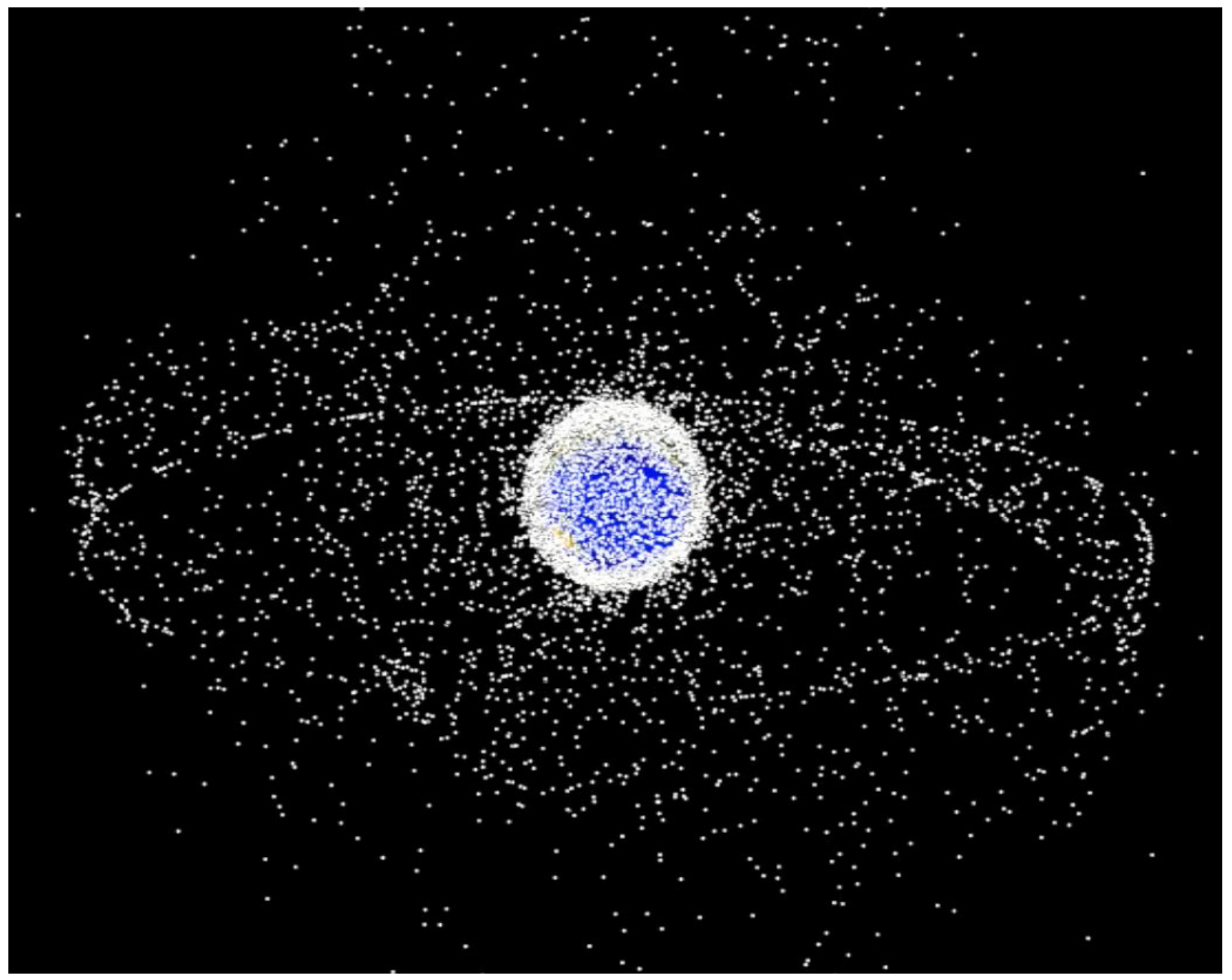
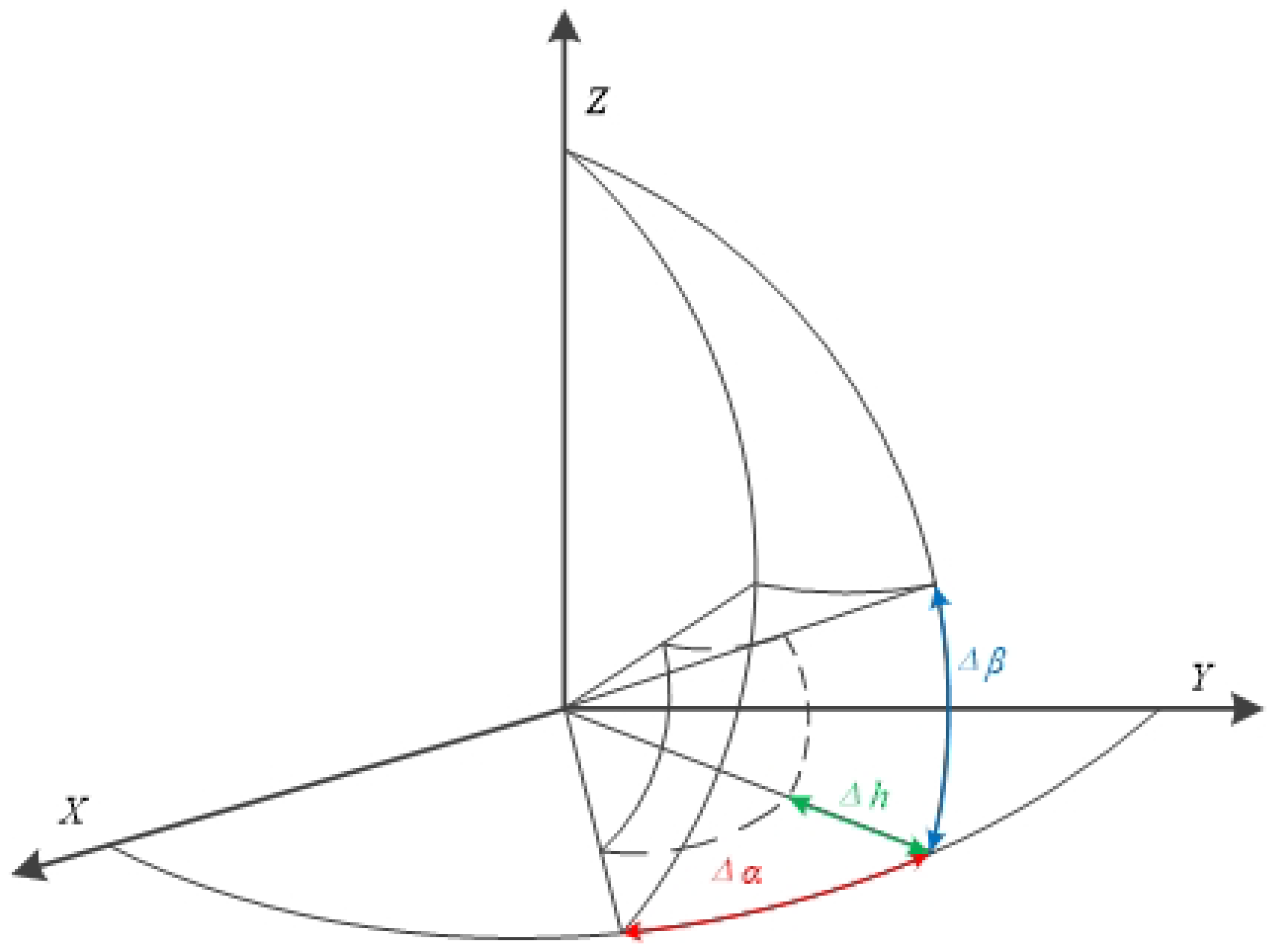
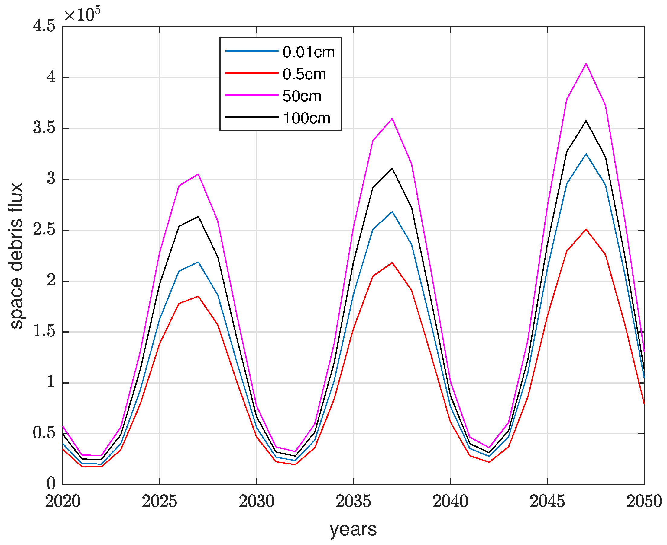
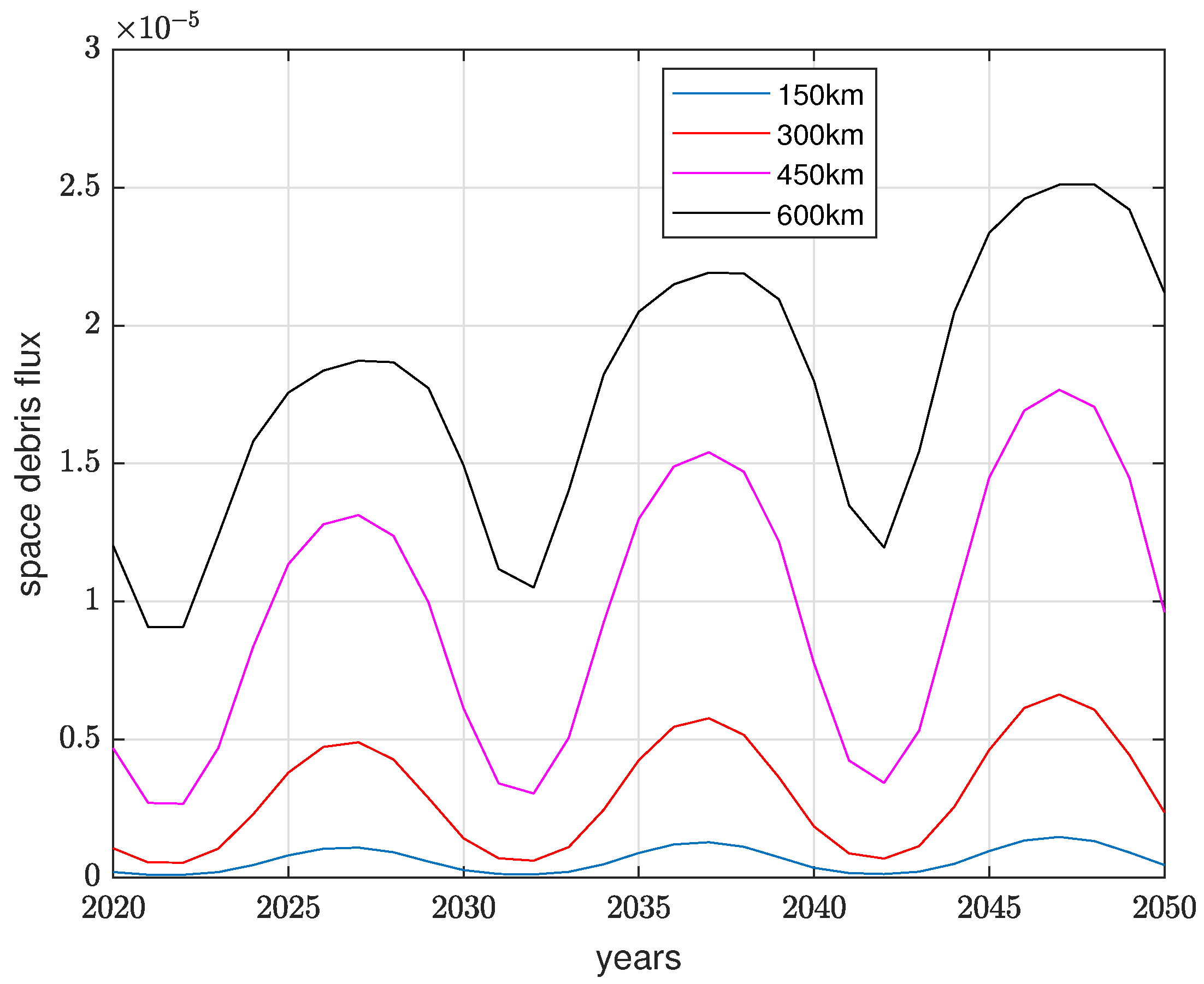
2.1. Space Orbital Debris Flux

As the variety of astronautic activities and the ability of the orbit-insert is enhanced, the numbers of on-orbit spacecrafts are significantly increased. Considering the limit of the accommodating capacity of orbital planes, the collision risk could also be increased and then accompany when a catastrophe occurs, such as satellites failure. Space orbital debris could be produced from retired spacecrafts, collision debris, and launch vehicles bodies; space particles are also included. According to the size of the orbital debris, it could be divided into “big” debris and “small” debris; the detriments are included in

Table 1. The scale and detriments of orbital debris.

Scale Range	Orbital Debris	Detriments and Influence
More than 1 cm	Big debris	Orbit changed; Structure damaged; Mission failed
Less than 1 cm	Small debris	Payload hurt; Performance degraded; Life shortened

.

Before calculating the collision probability of orbital debris, the debris space flux model should be built based on the space cells. The space orbital operation environment could be divided into multiple space unit cells by taking advantage of the orbital height, longitude, and latitude, as shown in Figure 2.

Let h be the orbital height, $\alpha$ be the longitude, and $\beta$ be the latitude. Assuming i is the object in the space environment, j is the space unit cell and $V_j$ is space volume of the cell. When the object i flies through the cell j, $t_{ji}$ is the flying time during the orbital period $T_i$; then, the space density ${\rho }_{ji}$ could be denoted by the following equation:

$${\rho }_{ji}=\frac{t_{ji}}{T_i{V}_j}$$

(1)

Taking into account the existence of N objects, the space density can be calculated by the following equation:

$${\rho }_j=\sum _{i=1}^N{\rho }_{ji}$$

(2)

Let ${\overrightarrow{v}}_{ji}$ be the flying-through velocity and $\overrightarrow{n}$ be the pointing unit vector of the cross profile, then the space cell flux can be computed by:

$$F_{ji}\left(\overrightarrow{n}\right)={\rho }_{ji}{\overrightarrow{v}}_{ji}$$

(3)

Given N objects, the above equation can be expressed by:

$$F_j\left(\overrightarrow{n}\right)=\sum _{i=1}^N{F}_{ji}\left(\overrightarrow{n}\right)$$

(4)

Assuming P is the point in the space unit cell and S is the infinitesimal element of a spatial spherical centered at P, then the solid angle $d{\mathsf{\Omega }}_{SP}$ from P to S is denoted by:

$$\underset{S}{\int \int ◯}d{\mathsf{\Omega }}_{SP}=4\pi$$

(5)

Furthermore, the total orbital debris cross profile flux can be calculated by the following equation:

$$F_j=\underset{S}{\int \int ◯}{F}_j\left(\overrightarrow{n}\right)d{\mathsf{\Omega }}_{SP}$$

(6)

The mega-constellation projects deploy satellites on the low earth orbit in most cases, so the influence of atmospheric drag cabnot be neglected; therefore, it is necessary to consider the solar radiant index when calculating space debris flux. It is difficult to forecast the solar radiant activity in the future but thiw is not the emphasis of this article; the solar radiant factor can be approximately computed by:

$$RF=75cos\left\{a\left(y-b\right)+0.35sin\left[a\left(y-b\right)\right]\right\}+145$$

(7)

In the equation, let $a=0.001696$, $b=$ 44,605, and y be the modified Julian date. The relationship between space debris flux and different size of debris varying by years can be seen in Figure 3; the relationship between the space debris flux and different orbital heights varying by years can be seen in Figure 4.

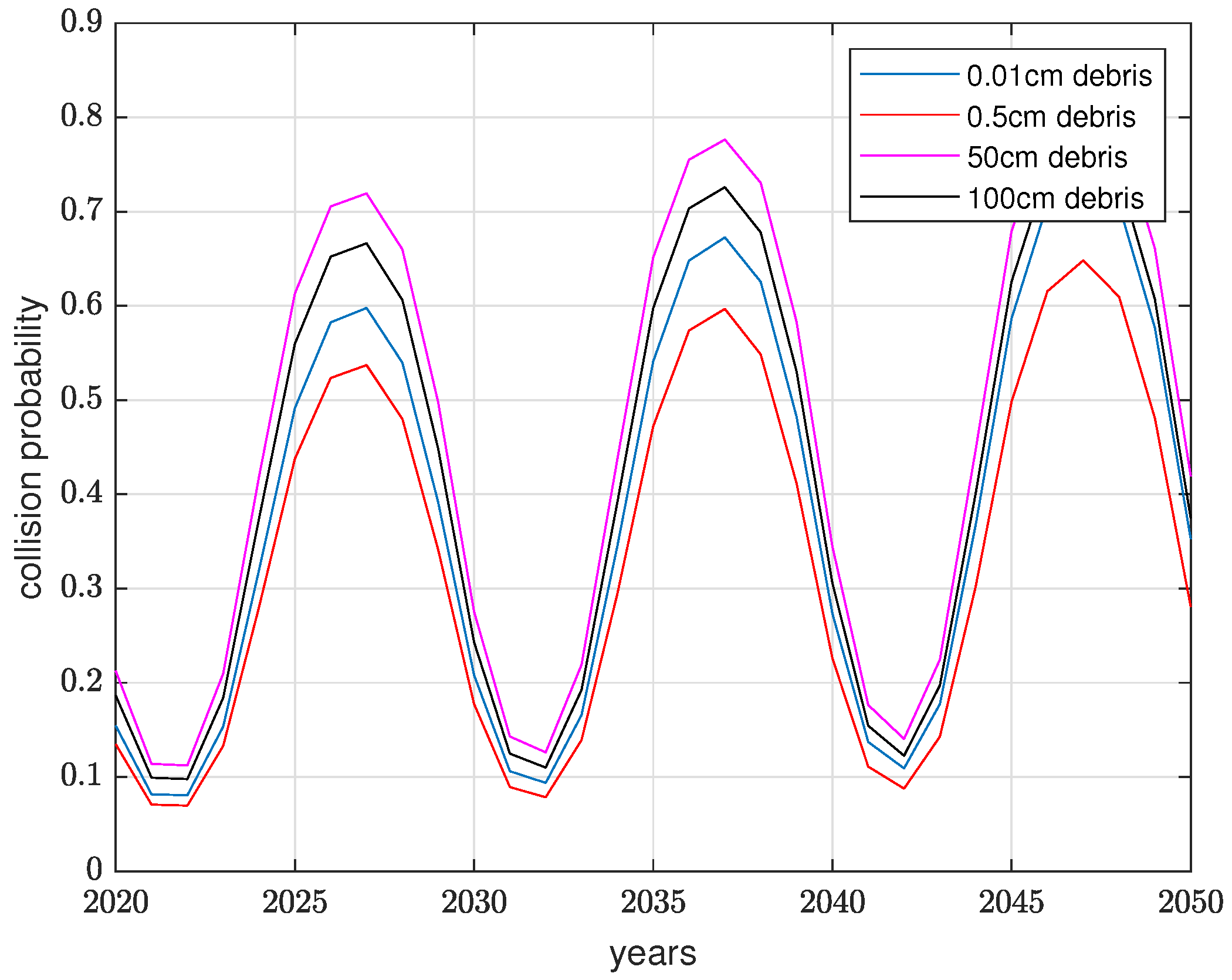
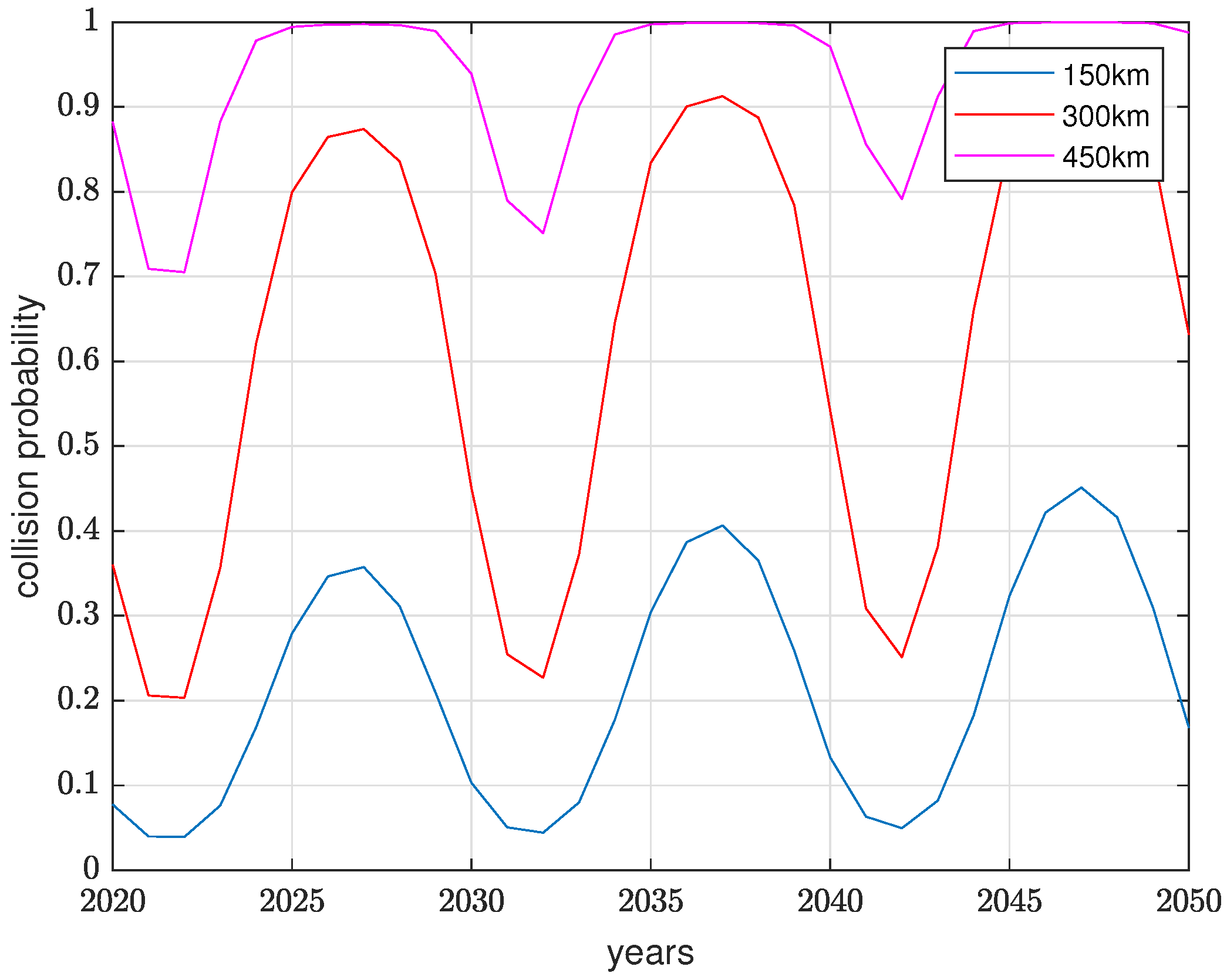
2.2. Collision Probability Analysis

During the operation time of on-orbit satellites, the likelihood of a collision between satellite and debris can be described as the collision probability. Let A be a cross-sectional area, assuming that the number N is proportional to the flux F, then the relationship equation is as follows:

$$N=F·A·T$$

(8)

Let n be the collision times during the flying-through time, $n=0,1,\cdots ,N$. The collision probability obeys the Poisson distribution, that is:

$$P_n=\frac{N^n{e}^{-N}}{n!}$$

(9)

No collision occurred when $n=0$, $P_0=exp\left(-N\right)$ at this time, so the collision probability is shown as follows:

$$P=1-P_0=1-exp\left(-N\right)$$

(10)

The relationship between the collision probability and different sizes of debris varying by years can be seen in Figure 5, and the relationship between the collision probability and different orbital heights varying by years can be seen in Figure 6.

As seen in Figure 5 and Figure 6, the trends of space orbital flux and collision probability mainly depend on the solar radiant activities. With orbital height increased and debris size enlarged, the probability would grow larger.

3. Markov Process of Staged Deployment

3.1. Definitions of Staged Strategy State Variables

Assuming that a mega-constellation consists of $n_t$ identical satellites, $n_t\in \left\{0,1,\cdots ,n_{max}\right\}$. By reason of the congestion problem on LEO, collisions would frequently occur during operation stages and the performance or utility would degrade; therefore, additional satellites need to be launched. The optimal deployment strategy is that the decision to launch arational number of satellites assures that the constellations follow normal operation sequentially and that the corresponding cost is minimized when the systems encounter malfunctions.

The number of on-orbit satellites $n_t$, along with the space collision probability $p_t$, forms the state space. The state variables obey the Markov property and the collision probability has three realization modes: decreased, maintained, and increased. Within time step t, the state variables could be expressed by $x_t=\left(s_t,p_t\right)$, $x\in \left\{0,1,\cdots \left(n_{max}+1\right)·\left(p_{max}+1\right)-1\right\}$.

Decision-makers should determine the satellite numbers to be launched during the time steps, assuming that the launch capability limit is $u_{max}$. Let $p_t=0$, $p_t=1$, $p_t=2$ express the modes of decreased, maintained, and increased, respectively. The transition matrix can be seen in

Table 2. The transition matrix of Markov process.

${\mathit{p}}_{\mathit{t}}$	$$\mathit{P}\left({\mathit{p}}_{\mathit{t}+\mathbf{1}}=\mathbf{0}\left|{\mathit{p}}_{\mathit{t}}\right.\right)$$	$$\mathit{P}\left({\mathit{p}}_{\mathit{t}+\mathbf{1}}=\mathbf{1}\left|{\mathit{p}}_{\mathit{t}}\right.\right)$$	$$\mathit{P}\left({\mathit{p}}_{\mathit{t}+\mathbf{1}}=\mathbf{2}\left|{\mathit{p}}_{\mathit{t}}\right.\right)$$
0	$p_{00}$	$p_{01}$	$p_{02}$
1	$p_{10}$	$p_{11}$	$p_{12}$
2	$p_{20}$	$p_{21}$	$p_{22}$

.

During the various stages of constellations’ deployment, satellites being launched successfully is the first consideration. The normal operation of satellites needs to be guaranteed after satellites are inserted into orbit.

No launch failures and no collisions are important prerequisites for constellation-staged deployments. Let $e_{vf}$ be the event for launch failure and $e_c$ be the event for collision, then the failure probability of a single satellite can be computed with the following equation:

$$P\left(e_{sf}\right)=P\left(e_{vf}\right)+P\left(e_{vf}^{-1}\right)·\left[P\left(e_c\right)·P\left(e_{sf}\left|e_c\right.\right)+P\left(e_c^{-1}\right)·P\left(e_{ef}\left|e_c^{-1}\right.\right)\right]$$

(11)

In this equation, $e_{*}^{-1}$ is the opposite event of the responding event *. Compared with other events, such as subsystems malfunction and maneuver faults, the failure probability is relative large when collisions occur. Assuming $\epsilon$ satellites fail after the first deployment, then the constellation system could not provide service for customers anymore; in other words, when $k\ge \epsilon$, the whole system fails, so the failure probability can be calulated by:

$$P=\sum _{k=\epsilon }^{n_{max}}\left\{C_{n_{max}}^k·P{\left(e_{sf}\right)}^k·{\left[1-P\left(e_{sf}\right)\right]}^{n_{max}-k}\right\}$$

(12)

3.2. Cost-Effectiveness Analysis of Deployment Strategy

When systems fail, the previous deployment stages cannot operate normally and the investment becomes a sunk cost, with the economic value also included. However, the cost could be accounted for by the failure probability when systems encounter partial malfunctions. Let $C_f$ be the failure cost, $C_{ex}$ be the cost of development and deployment in the previous stages, and $V_{co}$ be the economic value brought by the previous deployment; therefore, the cost expression could be denoted by:

$$C_f=\left\{\begin{array}{cc}{C}_{ex}+V_{eco}& k\ge \epsilon \\ P·\left(C_{ex}+V_{eco}\right)& k<\epsilon \end{array}\right.$$

(13)

During each time step t, let $C_{tot,t}$ be the total cost, $C_{lau,t}$ be the cost of an additional launch, $C_{ord,t}$ be the cost of ordering new satellites, and $C_{op,t}$ be the operation cost. The total cost is:

$$C_{tot,t}=C_{f,t}+C_{lau,t}+C_{ord,t}+C_{op,t}$$

(14)

Assuming $C_{ex}$ is constant, the rest of each part is denoted by:

$$\begin{array}{c}{V}_{eco}={\alpha }_{eco}·n_t\\ C_{lau,t}={\alpha }_{lau}·u_t\\ C_{ord,t}={\alpha }_{lau}·u_t\\ C_{op,t}={\alpha }_{op}·n_t\end{array}$$

(15)

In the above equations, ${\alpha }_{*}$ is the coefficient of each item.

Similar to the cost of each stage, the effectiveness analysis consists of two partsL:normal operation and malfunction. Therefore, the calculation equation is:

$$E_{tot,t}=\left\{\begin{array}{cc}{E}_{o{p}^{-1},t}& k\ge \epsilon \\ E_{op,t}& k<\epsilon \end{array}\right.$$

(16)

The net profit function $NP\left(n_t,p_t;u_t\right)$ in each time step t can be built by:

$$NP\left(n_t,p_t;u_t\right)=E_{tot,t}-C_{tot,t}=E_{tot,t}-\left(C_{f,t}+C_{lau,t}+C_{ord,t}+C_{op,t}\right)$$

(17)

The optimal strategy is the decision which could maximize the net profit, denoted by $u_t^{*}$. The calculation flow is shown in

Table 3. Optimal deployment strategy flow of finding.

The Solving Process of Net Profit Function
1: Set $N{P}_0\left(x\right)=0$
2: For $t=1:T$, $N{P}_{t+1}\left(x\right)=\underset{u_t}{max}E\left[NP\left(n_t,p_t;u_t\right)+N{P}_t\left(x\right)\right]$
3: Find $u_t^{*}$ and finish solving

.

4. Case Study

In this section, the Markov decision process is used to find the optimal strategy for the LEO mega-constellation.

4.1. Parameters of Simulation Model

Given the collision probability $p_t$, the Markov transition matrix was computed by space orbital debris flux, as shown in

Table 4. The transition matrix of collision probability.

${\mathit{p}}_{\mathit{t}}$	$$\mathit{P}\left({\mathit{p}}_{\mathit{t}+\mathbf{1}}=\mathbf{0}\left|{\mathit{p}}_{\mathit{t}}\right.\right)$$	$$\mathit{P}\left({\mathit{p}}_{\mathit{t}+\mathbf{1}}=\mathbf{1}\left|{\mathit{p}}_{\mathit{t}}\right.\right)$$	$$\mathit{P}\left({\mathit{p}}_{\mathit{t}+\mathbf{1}}=\mathbf{2}\left|{\mathit{p}}_{\mathit{t}}\right.\right)$$
0	0.4431	0.1053	0.4516
1	0.2483	0.0156	0.7361
2	0.0672	0.1693	0.7635

.

Based on historical data, the probability of aunch vehicle failure was denoted by $P\left(e_{vf}\right)=0.03$. Let the collision probability $P\left(e_{sf}\left|e_c\right.\right)=0.95$ because the consequencse would be severe when collisions occur during operation periods. Therefore, the probability due to a subsystem malfunction is relatively small, $P\left(e_{sf}\left|e_c^{-1}\right.\right)=0.03$.

Given the three realizations of the probability distribution, let $T=10$; then the probability is shown as in

Table 5. Collision probability within time steps.

${\mathit{p}}_{\mathit{t}}$	Collision Probability
$p_1$	$\left[0.2482;0.0153;0.7361\right]$
$p_2$	$\left[0.1632;0.1510;0.6854\right]$
$p_3$	$\left[0.1559;0.1355;0.7081\right]$
$p_4$	$\left[0.1503;0.1384;0.7108\right]$
$p_5$	$\left[0.1487;0.1383;0.7124\right]$
$p_6$	$\left[0.1481;0.1384;0.7129\right]$
$p_7$	$\left[0.1479;0.1384;0.7130\right]$
$p_8$	$\left[0.1478;0.1384;0.7131\right]$
$p_9$	$\left[0.1478;0.1384;0.7130\right]$
$p_{10}$	$\left[0.1477;0.1384;0.7130\right]$

.

Based on the collision probability within the time steps, the probability at different states was calculated, as shown in

Table 6. Collision probability during different states.

State	Collision Probability	Value
decreased	$P\left(e_c\left|p_t=0\right.\right)$	$1.7608\times {10}^{-4}$
maintained	$P\left(e_c\left|p_t=1\right.\right)$	$1.8471\times {10}^{-4}$
increased	$P\left(e_c\left|p_t=2\right.\right)$	$1.8723\times {10}^{-4}$

.

Assuming that the mega-constellation needs at least 30 satellites to operate normally in order to provide service for customers in the target region, the constellation consisted of 60 satellites and the upper limit of the launch capability was 10 satellites. Therefore, $u_t\in \left\{0,1,\cdots ,10\right\}$, $n_t\in \left\{10,11,\cdots ,60\right\}$, and the size of state space was 153, as shown in

Table 7. State space of Markov decision process.

State	Collision Probability
$x_t=0$	$\left(10,0\right)$
$x_t=1$	$\left(10,1\right)$
$x_t=2$	$\left(10,2\right)$
$x_t=3$	$\left(11,0\right)$
⋮	⋮
$x_t=151$	$\left(60,1\right)$
$x_t=152$	$\left(60,2\right)$

.

Other parameters related to economic value are shown as

Table 8. The data of simulation parameters.

Parameters	Value	Parameter	Value
$C_{ex}$	50,000	$E_{op}$	50,000
${\alpha }_{eco}$	600	${\alpha }_{lau}$	350
${\alpha }_{ord}$	600	${\alpha }_{op}$	30

, with units in millions.

There is an assumption that at least 30 satellites need to be operated on orbit to assure the system normal performance, so the boundary condition was $\epsilon =30$. Given the capability of launching additional satellites, the optimal deployment strategies are shown as Figure 7, considering different state variables $x_t$.

According to the simulation parameters, the optimal decision actions which are denoted as $u^{*}$ are shown as Figure 8. Four scenarios could be divided with different deployment stages.

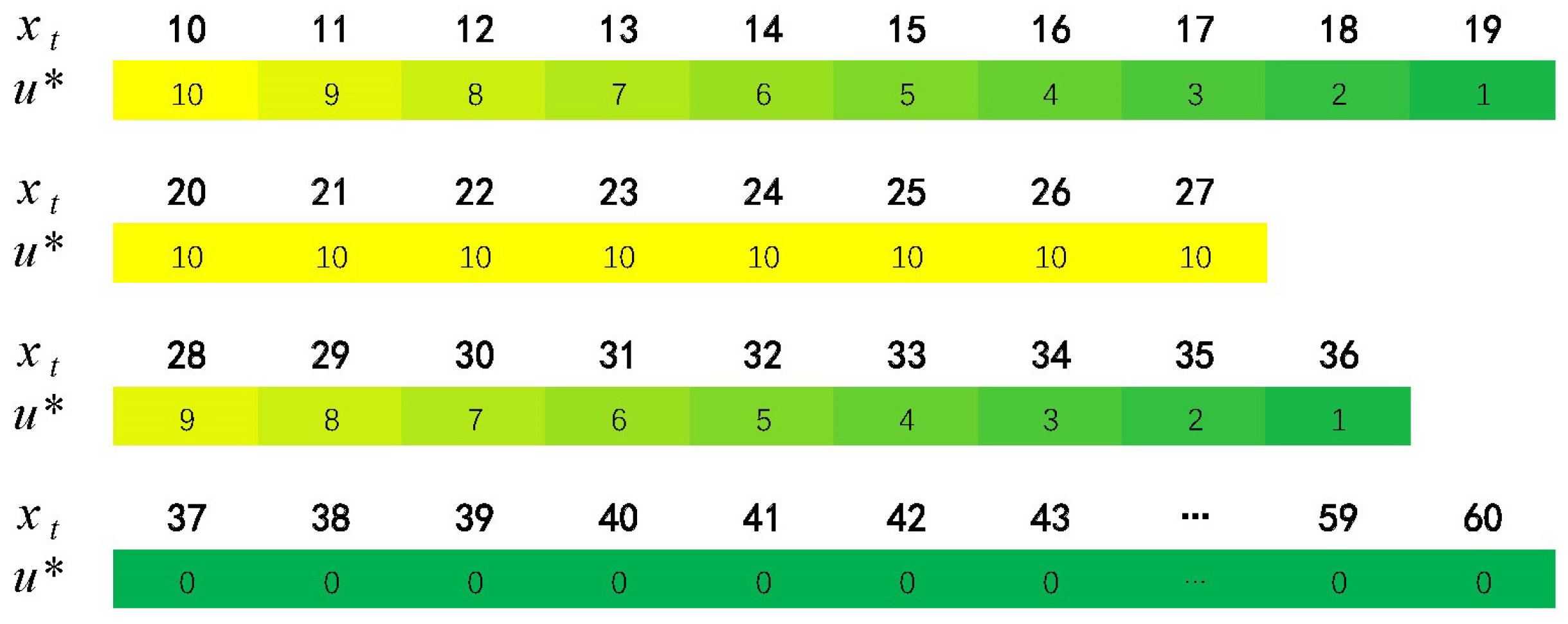
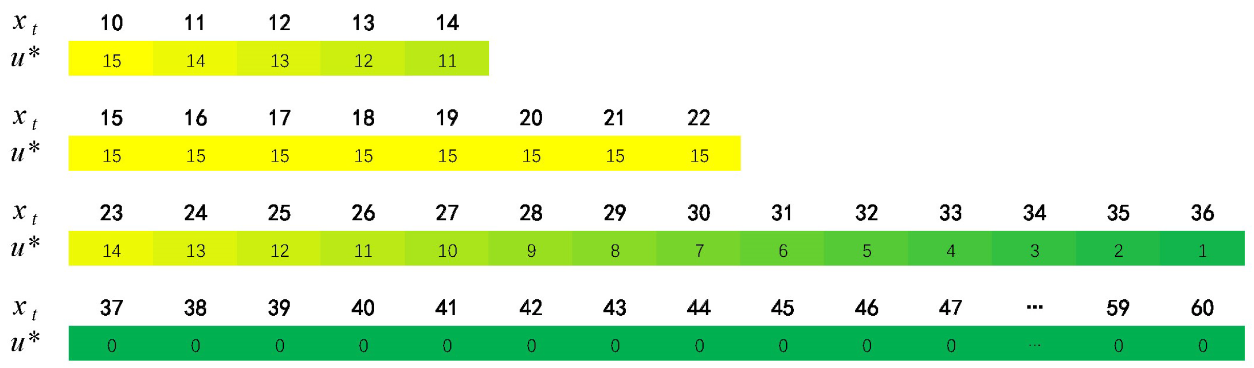
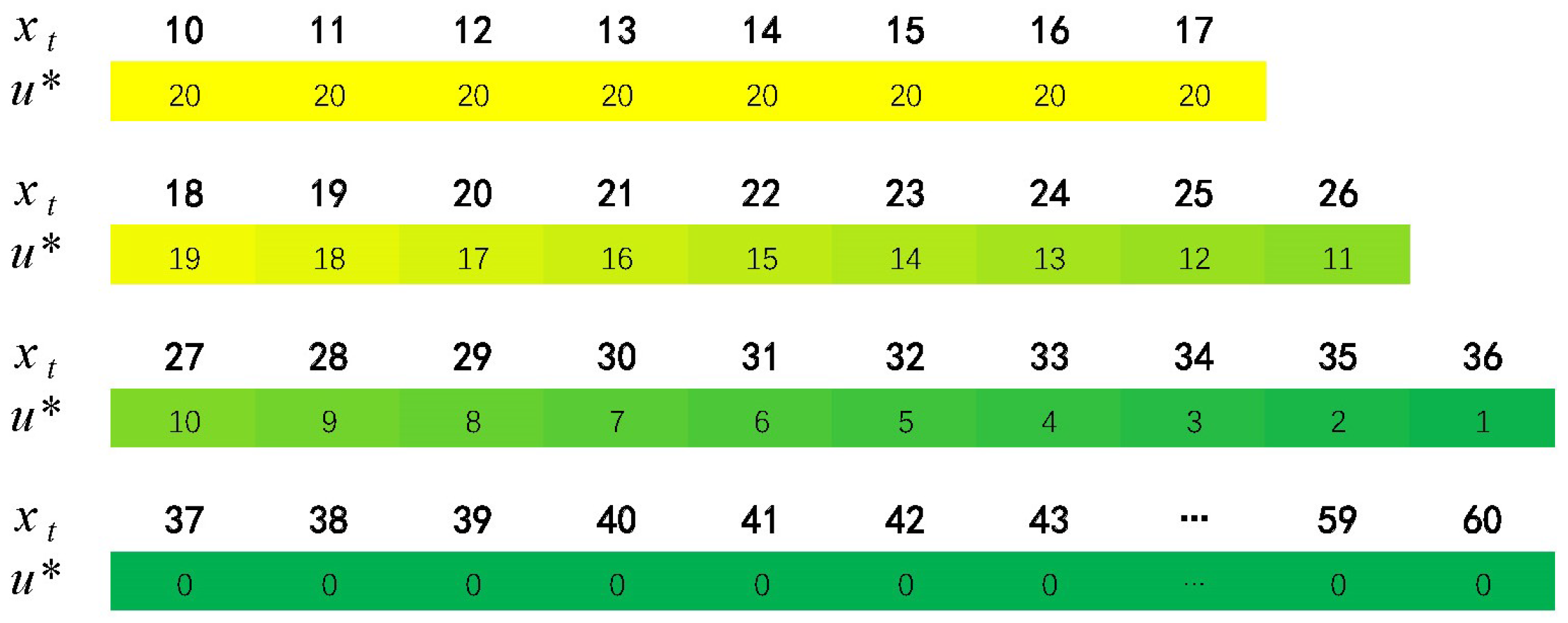
• 10∼19 satellites on-orbit operation. Given the boundary condition, the system could not provide a service in this stage. For the next deployment to progress successfully, 10 satellites would be launched at most, considering each cost item;
• 20∼27 satellites on-orbit operation. By reason of a malfunction such as collision and some faults, more satellites need to be launched into orbit for backups and the maximum capability of launching would be taken full advantage in this scenario;
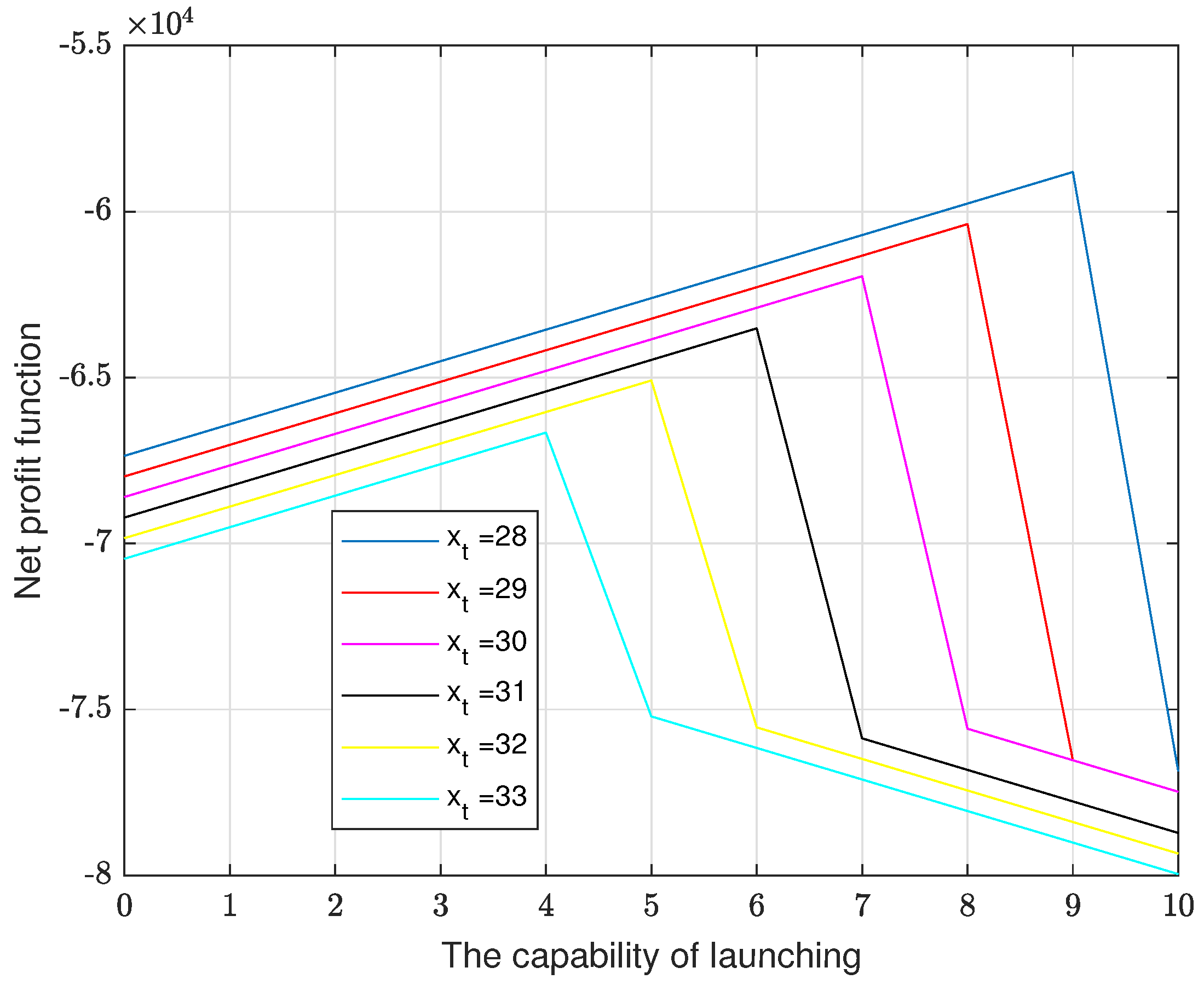
• 28∼36 satellites on-orbit operation. Based on the last scenario, the optimal decision assures 37 satellites on-orbit. For maximizing the net profit function, there is an incremental reduction during the deployment stages;
• 37∼60 satellites on-orbit operation. Satellites could not be launched anymore because the system would provide services and launching costs would not be covered by the system benefits.

The results of the upper limit of the launching capability are 15 and 20 satellites, as shown in Figure 9 and Figure 10, respectively.

As seen in Figure 9 and Figure 10, the case of 15 satellites is similar to the case of 10 satellites. For the case of 20 satellites, 3 scenarios were divided and the analysis process was same as the example case. The results of tge deployment decisions under different launch capabilities are summarized in

Table 9. Optimal deployment results under different scenarios.

Scenarios	10 Satellites Launched	15 Satellites Launched	20 Satellites Launched
Scenario 1	10–19 10–1	10–14 15–11	10–17 20
Scenario 2	20–27 10	15–22 15	18–36 19–1
Scenario 3	28–36 9–1	23–36 14–1	-
Scenario 4	≥37 0	≥37 0	≥37 0

.

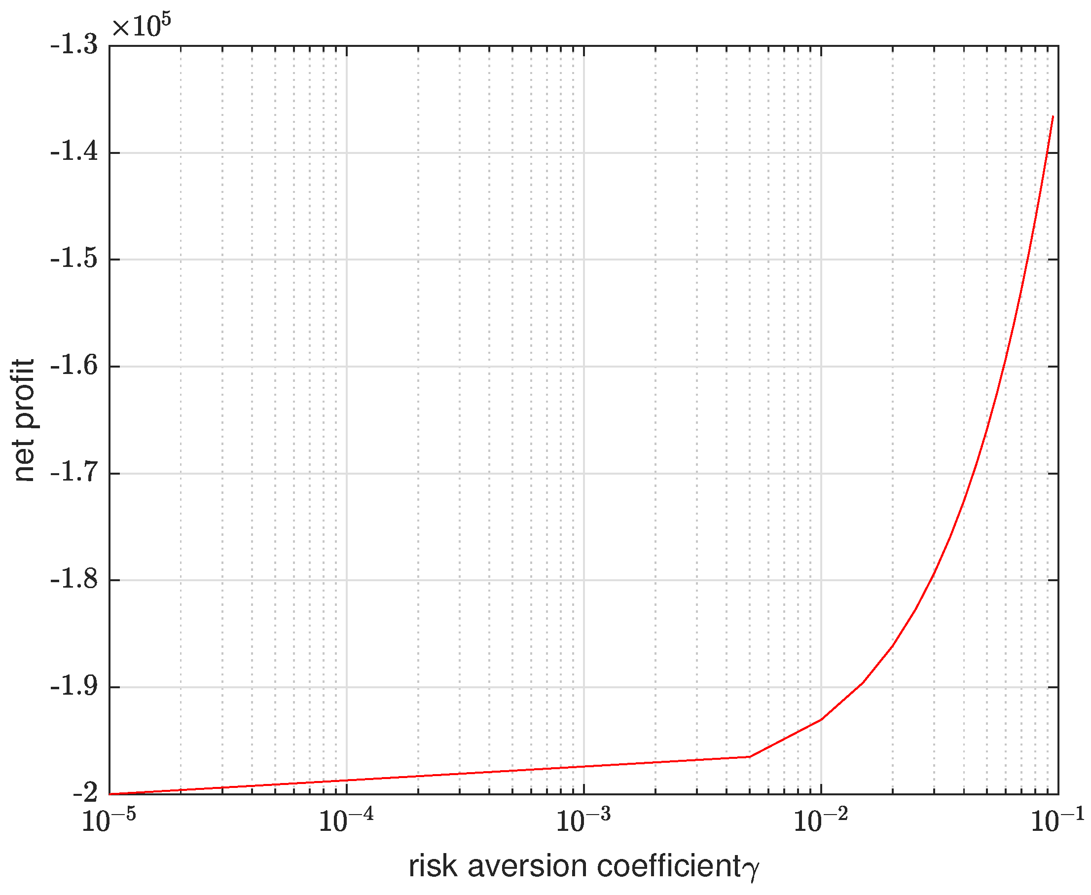
4.2. Sensitivity Analysis

Given the long development and deployment periods of a mega-constellation, there is much uncertainty. The risk aversion coefficient $\gamma$ is used for evaluating the degree that decision-makers could accept risk. Let $ER$ be the expected revenue and $C_{risk}$ be the cost of risk, then the utility function can be built with the following equation:

$$U=ER\left(x\right)-C_{risk}$$

(18)

When the value of tge utility function increased, the decision would be more satisfactory for investors. The standard deviation is denoted by $\sigma$, then the following relationship could be obtained with:

$$C_{risk}=\frac{1}{2}·\gamma ·{\sigma }^2$$

(19)

The risk of cost increases with the risk aversion coefficient increasing; the $\gamma$ can be denoted by:

$$\gamma \left(x\right)=-\frac{U^{″}\left(x\right)}{U^{\prime }\left(x\right)}$$

(20)

Therefore, the general form of the utility function can be built with the following equation:

$$U\left(x\right)=m-n·e^{-\gamma ·x}$$

(21)

In this equation, m and n are the constant fitting parameters. The relationship between the risk aversion coefficient and net profit is shown in Figure 11.

The higher the value of the risk aversion coefficient, the higher the degree of uncertainty is during the tge deployment process. This means that there iare more opportunities to make the net profit of the system better.

5. Conclusions

Mega-constellation projects have already been proposed and deployed by many countries and commercial organizations. They can more easily access space due to their advanced launch vehicles and rapid manufacture based on satellite platform. The LEO resources are more intense and congestion problems occurring are the direct consequence of more frequent human space activities. In this article, the space orbital flux model was built to calculate the space collision probability. When the constellation system encounters the collision problems, the performance is degraded or even malfunctions, so it is necessary to launch additional satellites to maintain the normal operations. The optimal deployment strategy was obtained through the Markov decision process. By launching moderate satellites, the system could continue providing services for customers and the net profit could be maximizd. The result could be the basis for decision making and the method shows the engineering applyication prospect to a certain degree.

References

1. Giordani, M.; Zorzi, M. Non-terrestrial networks in the 6G era: Challenges and opportunities. IEEE Netw. 2021, 35, 244–251. [Google Scholar] [CrossRef]
2. Portillo, I.; Cameron, B.; Crawley, E. A technical comparison of three low earth orbit satellite constellation systems to provide global broadband. Acta Astronaut. 2019, 159, 123–135. [Google Scholar] [CrossRef]
3. Navabi, M.; Hamrah, R. Close approach analysis of space objects and estimation of satellite-debris collision probability. Aircr. Eng. Aerosp. Technol. Int. J. 2015, 87, 483–492. [Google Scholar] [CrossRef]
4. Shi, K.; Liu, C.; Sun, Z. Coupled Orbit-Attitude Dynamics and Trajectory Tracking Control for Spacecraft Electromagnetic Docking. Appl. Math. Model. 2022, 101, 553–572. [Google Scholar] [CrossRef]
5. Liu, C.; Yue, X.; Zhang, J. Active Disturbance Rejection Control for Delayed Electromagnetic Docking of Spacecraft in Elliptical Orbits. IEEE Trans. Aerosp. Electron. Syst. 2022, 58, 2257–2268. [Google Scholar] [CrossRef]
6. Liu, C.; Yue, X.; Shi, K. Spacecraft Attitude Control: A Linear Matrix Inequality Approach, 1st ed.; Science Press: Beijing, China, 2022; pp. 15–27. [Google Scholar]
7. McKnight, D.; Pentino, F. New insights on the orbital debris collision hazard at GEO. Acta Astronaut. 2013, 85, 73–82. [Google Scholar] [CrossRef]
8. Shajiee, S. Probability of collision and risk minimization of orbital debris on the Galileo satellite constellation. In Proceedings of the 54th International Astronautical Congress of the International Astronautical Federation, the International Academy of Astronautics, and the International Institute of Space Law, Bremen, Germany, 29 September–3 October 2004. [Google Scholar]
9. May, S.; Gehly, S.; Carter, B. Space debris collision probability analysis for proposed global broadband constellations. Acta Astronaut. 2018, 151, 445–455. [Google Scholar] [CrossRef]
10. Liu, M.; Zhu, Z. Simulation of collision probability between space station and space debris and structure failure probability. Int. J. Space Sci. Eng. 2017, 4, 253–269. [Google Scholar] [CrossRef]
11. Torky, M.; Hassanein, A.; Fiky, A. Analyzing space debris flux and predicting satellites collision probability in LEO orbits based on Petri nets. IEEE Access 2019, 7, 83461–83473. [Google Scholar] [CrossRef]
12. Fleischmann, M.; Kuik, R. On optimal inventory control with independent stochastic item returns. Eur. J. Oper. Res. 2003, 151, 25–37. [Google Scholar] [CrossRef]
13. Bergamini, E.; Jacobone, F.; Morea, D. The Increasing Risk of Space Debris Impact on Earth: Case Studies, Potential Damages, International Liability Framework and Management Systems. In Enhancing CBRNE Safety & Security: Proceedings of the SICC 2017 Conference: Science as the First Countermeasure for CBRNE and Cyber Threats, Rome, Italy, 4 October 2018; Springer International Publishing: Berlin, Germany, 2018. [Google Scholar]
14. Johnson, L. Orbital debris: The growing threat to space operations. In Proceedings of the 33rd Annual Guidance and Control Conference, Huston, TX, USA, 25 August 2013. [Google Scholar]
15. Johnson, L. Instability of the present LEO satellite populations. Adv. Space Res. 2008, 41, 1046–1053. [Google Scholar]
16. Pardini, C.; Anselmo, L. Review of past on-orbit collisions among cataloged objects and examination of the catastrophic fragmentation concept. Acta Astronaut. 2014, 100, 30–39. [Google Scholar] [CrossRef]
17. Pardini, C.; Anselmo, L. Revisiting the collision risk with cataloged objects for the Iridium and COSMO-SkyMed satellite constellations. Acta Astronaut. 2017, 134, 23–32. [Google Scholar] [CrossRef]
18. Lewis, H.; Radtke, J.; Rossi, A. Sensitivity of the space debris environment to large constellations and small satellites. J. Br. Interplanet. Soc. 2017, 70, 105–117. [Google Scholar]
19. Virgili, B.; Krag, H.; Lewis, H. Mega-constellations, small satellites and their impact on the space debris environment. In Proceedings of the 67th International Astronautical Congress, Guadalajara, Mexico, 10 August 2016. [Google Scholar]
20. Pereira, H.; Marques, C. An analytical review of irrigation efficiency measured using deterministic and stochastic models. Agric. Water Manag. 2017, 184, 28–35. [Google Scholar] [CrossRef]
21. Wagner, R.; Radovilsky, Z. Optimizing boat resources at the US Coast Guard: Deterministic and stochastic models. Oper. Res. 2012, 60, 1035–1049. [Google Scholar] [CrossRef]
22. Budianto, A.; Olds, R. Design and deployment of a satellite constellation using collaborative optimization. J. Spacecr. Rocket. 2004, 41, 956–963. [Google Scholar] [CrossRef]
23. De Weck, O.; De Neufville, R.; Chaize, M. Staged deployment of communications satellite constellations in low earth orbit. J. Aerosp. Comput. Inform. Commun. 2004, 1, 119–136. [Google Scholar] [CrossRef]
24. Gökbayrak, E.; Kayış, E. Single item periodic review inventory control with sales dependent stochastic return flows. Int. J. Prod. Econ. 2023, 255, 108699–108707. [Google Scholar] [CrossRef]
25. Baeza, V.; Lagunas, E.; Al-Hraishawi, H.; Chatzinotas, S. An Overview of Channel Models for NGSO Satellites. In Proceedings of the 2022 IEEE 96th Vehicular Technology Conference, London, UK, 26 September 2022. [Google Scholar]
Figure 1. The current status of LEO environment.
Symmetry 15 01024 g001
Figure 2. Space unit cell of orbital debris flux model.
Symmetry 15 01024 g002
Figure 3. The influence of debris size for space debris flux as years.
Symmetry 15 01024 g003
Figure 4. The influence of orbital height for space debris flux as years.
Symmetry 15 01024 g004
Figure 5. The influence of debris size for collision probability as years.
Symmetry 15 01024 g005
Figure 6. The influence of orbital height for collision probability as years.
Symmetry 15 01024 g006
Figure 7. The optimal deployment decision of state variables.
Symmetry 15 01024 g007
Figure 8. The optimal deployment decision of state variables with 10 satellites launched additionally.
Symmetry 15 01024 g008
Figure 9. The optimal deployment decision with 15 additional satellites launched.
Symmetry 15 01024 g009
Figure 10. The optimal deployment decision with 20 additional satellites launched.
Symmetry 15 01024 g010
Figure 11. The relationship between risk aversion coefficient and net profit.
Symmetry 15 01024 g011