Article

Generalized AB-Fractional Operator Inclusions of Hermite–Hadamard’s Type via Fractional Integration

by
Bandar Bin-Mohsin
1,
Muhammad Uzair Awan
2,*,
Muhammad Zakria Javed
2,
Awais Gul Khan
2,
Hüseyin Budak
3,
Marcela V. Mihai
4 and
Muhammad Aslam Noor
5
1
Department of Mathematics, College of Science, King Saud University, Riyadh 11451, Saudi Arabia
2
Department of Mathematics, Government College University, Faisalabad 38000, Pakistan
3
Department of Mathematics, Faculty of Science and Arts, Düzce University, Duzce 81620, Turkey
4
Department Scientific-Methodical Sessions, Romanian Mathematical Society-Branch Bucharest, Academy Street no. 14, RO-010014 Bucharest, Romania
5
Department of Mathematics, COMSATS University Islamabad, Islamabad 4000, Pakistan
*
Author to whom correspondence should be addressed.
Symmetry 2023, 15(5), 1012; https://doi.org/10.3390/sym15051012
Submission received: 21 March 2023 / Revised: 26 April 2023 / Accepted: 27 April 2023 / Published: 1 May 2023
(This article belongs to the Special Issue Symmetry in Functional Equations and Analytic Inequalities III)

Abstract

:
The aim of this research is to explore fractional integral inequalities that involve interval-valued preinvex functions. Initially, a new set of fractional operators is introduced that uses the extended generalized Mittag-Leffler function E μ , α , l γ , δ , k , c ( τ ; p ) as a kernel in the interval domain. Additionally, a new form of Atangana–Baleanu operator is defined using the same kernel, which unifies multiple existing integral operators. By varying the parameters in E μ , α , l γ , δ , k , c ( τ ; p ) , several new fractional operators are obtained. This study then utilizes the generalized AB integral operators and the preinvex interval-valued property of functions to establish new Hermite–Hadamard, Pachapatte, and Hermite–Hadamard–Fejer inequalities. The results are supported by numerical examples, graphical illustrations, and special cases.

1. Introduction and Preliminaries

Let us rewrite the notion of the convex set and convex functions.
Definition 1.
A C R is said to be a convex if:
( 1 τ ) v 1 + τ v 2 C v 1 , v 2 C , τ [ 0 , 1 ] .
Definition 2.
Let C R be a convex set. A function f : C R is said to be convex, if
f ( ( 1 τ ) v 1 + τ v 2 ) ( 1 τ ) f ( v 1 ) + τ f ( v 2 ) , v 1 , v 2 C , τ [ 0 , 1 ] .
The basic concepts of convex analysis have been extensively explored in various directions due to their wide-ranging applications. The theory of convex functions is a fascinating subject in analysis, as it finds applications in diverse fields, such as engineering, separation theorems, optimization theory, differential equations, and more. Moreover, it has strong connections with the theory of inequalities, and many inequalities can be directly derived from the definition of convex functions. One of the most intriguing inequalities that emerges from the study of convex functions is the Jensen inequality.
Let f : I = [ v 1 , v 2 ] R be a convex function, then
f i = 1 n u i x i i = 1 n u i f ( x i ) , x i I , u i 0 , i = 1 , 2 , 3 , , n , i = 1 n u i = 1 .
The Hermite–Hadamard inequality is a well-known inequality that serves as a necessary and sufficient condition for a convex function. It is formulated as follows:
Let f : I = [ v 1 , v 2 ] R be a convex function, then
f v 1 + v 2 2 1 v 2 v 1 v 1 v 2 f ( x ) d x f ( v 1 ) + f ( v 2 ) 2 , τ [ 0 , 1 ] .
Various generalizations, extensions, and refinements of convexity have been proposed in the literature, utilizing diverse weighted means such as harmonic convexity and geometric convexity, among others. For more information, refer to [1,2,3]. Moving on, let us now consider another generalization of convexity. We will revisit the concept of invex sets and preinvex functions.
Definition 3
([4]). A set K is considered invex in relation to a bifunction ζ : K × K R if
x + τ ζ ( y , x ) K , x , y K , τ [ 0 , 1 ] .
Definition 4
([4]). If f is a function defined on an invex set K, then it is considered preinvex with respect to the bifunction ζ ( · , · ) if
f ( x + τ ζ ( y , x ) ) ( 1 τ ) f ( x ) + τ f ( y ) , x , y K , τ [ 0 , 1 ] .
In their previous work, Mohan and Neogy [5] introduced Condition C, which has proven to be highly useful and plays a significant role in establishing some of our main results. For the sake of completeness, we will recall Condition C as follows:
Let K R be an invex set with respect to a bifunction ζ ( . , . ) . Then, for any τ [ 0 , 1 ] and x , y A , the following condition holds:
ζ ( y , y + τ ζ ( x , y ) ) = τ ζ ( x , y ) ζ ( x , y + τ ζ ( x , y ) ) = ( 1 τ ) ζ ( x , y ) .
Moreover,
ζ ( y + τ 2 ζ ( x , y ) , y + τ 1 ζ ( x , y ) ) = ( τ 2 τ 1 ) ζ ( x , y ) ,
for any τ 1 , τ 2 [ 0 , 1 ] .
Interval analysis is a unique implementation of set-valued analysis that utilizes a nonprobabilistic approach. It is undoubtedly an essential tool for both pure and applied mathematics. Initially, the interval analysis technique was developed to evaluate error estimates for finite state machines. Over the past fifty years, it has been utilized in mathematical models to address interval-uncertain structural systems. The technique has significant applications in various fields, including automatic error analysis, computer graphics, neural networking, and optimization.
The notion of interval-valued convexity was first introduced by Breckner [6]. Furthermore, we denote the space of all real intervals and space of intervals of positive real numbers by R I and R I + .
Definition 5.
Let f : I = [ v 1 , v 2 ] R I + , which is said to to be an interval-valued convex function, if
f ( ( 1 τ ) v 1 + τ v 2 ) ( 1 τ ) f ( v 1 ) + τ f ( v 2 ) , τ [ 0 , 1 ] .
The following concept to consider is the preinvexity of interval values.
Definition 6
([7]). An interval-valued function f : K R I + , defined on an invex set K R , is classified as an interval-valued preinvex function if and only if
f ( x + τ ζ ( y , x ) ) ( 1 τ ) f ( x ) + τ f ( y ) ,
which holds true for each x , y K and for all τ [ 0 , 1 ] .
Calculus is concerned with the investigation of derivatives and their implications in measuring the rate of change in a dependent variable relative to an independent variable. Fractional calculus, however, extends the concept of derivatives to noninteger orders. The roots of fractional calculus can be traced back to a conversation between Leibniz and L’Hospital about non-integer order derivatives. While the first-order derivative corresponds to the slope of a tangent at a point and the second-order derivative indicates the curvature, fractional calculus allows us to observe very small changes between two integer order derivatives in various phenomena. Fractional calculus is widely regarded as a powerful tool for describing real-life models, and its impact is indelible due to its wide range of applications in fields such as viscoelasticity, quantum mechanics, relativity theory, engineering, and more. Ongoing research in this area focuses on the development of new fractional operators and the generalization of existing results.
Let us now review some fundamental facts and concepts.
Definition 7
([8]). Defined as E α ( · ) , the Mittag-Leffler function is given by
E α ( τ ) = n = 0 τ n Γ ( α n + 1 ) ,
where τ , α C , R ( α ) > 0 and Γ ( · ) is the gamma function.
Definition 8
([8]). Let μ , α , l , γ , c C , where R ( μ ) , R ( α ) , and R ( l ) are greater than zero, and R ( c ) > γ > 0 . Let p 0 , δ > 0 , and 0 < k δ + R ( μ ) . With these conditions, the extended generalized Mittag-Leffler function E μ , α , l γ , δ , k , c ( τ ; p ) can be defined as follows:
E μ , α , l γ , δ , k , c ( τ ; p ) = n = 0 β p ( γ + n k , c γ ) β ( γ , c γ ) ( c ) n k Γ ( μ n + α ) τ n ( l ) n δ ,
where β p ( · , · ) is defined by
β p ( x , y ) = 0 1 τ x 1 ( 1 τ ) y 1 e p τ ( 1 τ ) d τ ,
and ( c ) n k : = Γ ( c + n k ) Γ ( c ) .
Definition 9
([8]). Assume that w , μ , α , l , γ , c C , where R ( μ ) , R ( α ) , and R ( l ) are greater than zero, and R ( c ) > γ > 0 . Let p 0 , δ > 0 , and 0 < k δ + R ( μ ) . Consider f L 1 [ v 1 , v 2 ] and x [ v 1 , v 2 ] . Then, we can define the generalized left-hand-side fractional integral operator containing Mittag-Leffler function E μ , α , l γ , δ , k , c ( τ ; p ) as follows:
ϵ μ , α , l , w , v 1 + γ , δ , k , c { f ( x ; p ) } = v 1 x ( x τ ) α 1 E μ , α , w , l γ , δ , k , c ( w ( x τ ) μ ; p ) f ( τ ) d τ .
The following expression defines the generalized right-hand-side fractional integral operator:
ϵ μ , α , l , w , v 2 γ , δ , k , c { f ( x ; p ) } = x v 2 ( τ x ) α 1 E μ , α , w , l γ , δ , k , c ( w ( τ x ) μ ; p ) f ( τ ) d τ .
Atangana and Baleanu introduced a set of new integrals in [9], which are commonly referred to as Atangana–Baleanu fractional integrals.
Definition 10.
The fractional integral associated with the new nonlocal kernel of a mapping f L 1 ( v 1 , v 2 ) is defined in the following manner:
v 1 A B I τ α f ( τ ) = 1 α B ( α ) f ( τ ) + α B ( α ) Γ ( α ) v 1 τ f ( x ) ( τ x ) α 1 d x , w h e r e v 2 > v 1 , α [ 0 , 1 ] .
The expression for the right-hand side of the integral operator is as follows:
A B I v 2 α f ( τ ) = 1 α B ( α ) f ( τ ) + α B ( α ) Γ ( α ) τ v 2 f ( x ) ( x τ ) α 1 d x .
Here, Γ ( α ) is the gamma function. B ( α ) > 0 is called the normalization function satisfying the condition B ( 0 ) = B ( 1 ) = 1 . For more detail, see [9].
Definition 11
([10]). Assume that f ( x ) = [ f ̲ ( x ) , f ¯ ( x ) ] , x Λ 0 is the interval-valued function, where Λ 0 is the interior of Λ R . We call f ( x ) Lebesgue-integrable if the functions f ̲ ( x ) as well as f ¯ ( x ) are both measurable along with the Lebesgue integrable defined over Λ 0 . Furthermore, we can write v 1 v 2 f ( x ) d x as follows:
v 1 v 2 f ( x ) d x = v 1 v 2 f ̲ ( x ) d x , v 1 v 2 f ¯ ( x ) d x .
Fractional calculus has attracted a lot of attention from researchers who seek to extend and improve fundamental inequalities. In 2012, Sarikaya et al. [11] introduced fractional concepts to the well-known Hermite and Hadamard inequality, which opened the door for further research in mathematical analysis. Since then, many studies on inequalities have emerged using fractional calculus. For example, Muhammad et al. [12,13] have established new versions of the Hermite–Hadamard-type inequalities involving the tempered fractional integral operator and some fractional mid-point inequalities of the Hermite–Hadamard type, respectively. Akdemir et al. [14] have investigated Chebyshev-type inequalities using generalized fractional integral operators. Set et al. [15] have studied integral inequalities using the Atangana–Baleanu fractional operator. Recently, Butt et al. [16] have derived improved versions of inequalities using the concept of harmonically exponential convex functions.
In 2012, the concept of interval-valued functions and the generalized Hukuhara derivative were introduced by authors [17] to calculate some Ostrowski-like inequalities. Meanwhile, Chalco-Cano et al. [18] derived Ostrowski-type inequalities using interval-valued mapping and presented some applications to numerical integration. In 2017, Costa et al. [19] established integral inclusions involving fuzzy interval-valued functions. In 2018, Authors et al. [20] studied integral inequalities involving the interval-valued property of functions. Zhang et al. [21] described the relationship between vector interval-valued problems and associated variational inequalities. Zhao et al. [22,23] proved Jensen- and Hermite–Hadamard-type inequalities associated with a class of convexity known as interval-valued h-convex functions and Chebyshev-type inequalities for interval-valued functions, respectively.
Budak et al. established fractional Hermite–Hadamard inequalities for interval-valued convex functions in [24], while Abdeljawad et al. derived generalized Hermite–Hadamard-type inequalities using interval-valued p-convexity in the fractional domain in [25]. Khan et al. utilized the concept of generalized fuzzy interval-valued functions and order relation to obtain Hermite–Hadamard-type inequalities in [26], and Liu et al. studied fractional analogs of these inequalities through interval-valued convexity in [27]. In [28], Younus et al. introduced a novel approach to investigate integral inequalities.
Recently, Kara et al. demonstrated coordinated inclusions of the Hermite–Hadamard type involving a generalized fractional operator in [29]. In [30,31], Kalsoom et al. derived ( p , q ) analogs of Hermite–Hadamard inequalities utilizing interval-valued convexity, and they also established mid-point-type inequalities that involve the Pompeiu-Hausdroff distance between intervals. They further discussed Hermite–Hadamard–Fejer-type inequalities for harmonically interval-valued h-convex functions. Finally, Afzal et al. introduced the concept of the Godunova–Levin ( h 1 , h 2 ) interval-valued convexity in [32] and derived new generalized Jensen- and Hermite–Hadamard-type inequalities. In [33], Bin-Mohsin et al. generalized the idea of LR-interval-valued convexity involving a β -connected set and derived some novel inequalities in the frame of fractional calculus. Bin-Mohsin and colleagues [34] explored the idea of harmonically co-ordinated interval-valued convex mappings and generalized fractional operators and developed some fundamental inequalities as applications. Khan et al. [35] formulated some weighted integral inequalities through generalized interval-valued convexity. Stojiljkovic and colleagues [36] examined some new inclusion relations incorporated with classical Riemann–Liouville fractional operators and convex mappings.
With inspiration from the above mentioned works in [22,23,24], our aim is to establish a new generalization of AB-fractional operators by utilizing the seven-parameter Mittag-Leffler functions as a nonsingular kernel in the setting of fractional interval-valued calculus. The main theme of our work is to introduce novel versions of Hermite–Hadamard’s inequality, Pachpatte’s inequality, and its weighted form named Hermite–Hadamard–Fejer inequality by leveraging the generalized interval-valued Mittag-Leffler fractional AB-integrals and the class of interval-valued preinvex functions. Some numeric examples and graphical illustrations will be provided to authenticate primary results. Then, we will describe some novel and exciting consequences of the main definitions and results. This paper aims to stimulate the curiosity of researchers interested in this field by presenting its unique ideas and techniques.

2. Main Results

In the proceeding section, we develop a new family of fractional operators that is described as:
Definition 12.
Assuming that f : [ v 1 , v 2 ] R I is an interval-valued function with f ( x ) = [ f ̲ ( x ) , f ¯ ( x ) ] , where the functions f ̲ ( x ) and f ¯ ( x ) are both Riemann-integrable and defined on the interval [ v 1 , v 2 ] , the corresponding interval-valued left-sided and right-sided Mittag-Leffler fractional AB-integrals are defined as follows:
ϵ μ , α , l , w , v 1 + γ , δ , k , c { f ( x ; p ) } = v 1 x ( x τ ) α 1 E μ , α , w , l γ , δ , k , c ( w ( x τ ) μ ; p ) f ( τ ) d τ .
The generalized right-hand-side fractional integral operator is given as follows:
ϵ μ , α , l , w , v 2 γ , δ , k , c { f ( x ; p ) } = x v 2 ( τ x ) α 1 E μ , α , w , l γ , δ , k , c ( w ( τ x ) μ ; p ) f ( τ ) d τ .
where
ϵ μ , α , l , w , v 1 + γ , δ , k , c { f ( x ; p ) } = ϵ μ , α , l , w , v 1 + γ , δ , k , c { f ̲ ( x ; p ) } , ϵ μ , α , l , w , v 1 + γ , δ , k , c { f ¯ ( x ; p ) } .
and
ϵ μ , α , l , w , v 2 γ , δ , k , c { f ( x ; p ) } = ϵ μ , α , l , w , v 2 γ , δ , k , c { f ̲ ( x ; ) } , ϵ μ , α , l , w , v 2 γ , δ , k , c { f ¯ ( v 1 ; p ) } .
Now, we discuss some special cases of Definition 12.
  • Choosing p = 0 , we then obtain a new fractional operator of the Salim–Faraj type.
    ϵ μ , α , l , w , v 1 + γ , δ , k , { f ( x ) } = v 1 x ( x τ ) α 1 E μ , α , w , l γ , δ , k ( w ( x τ ) μ ) f ( τ ) d τ .
    The right-hand side of the new fractional integral operator of the Salim–Faraj type is given as follows:
    ϵ μ , α , l , w , v 2 γ , δ , k { f ( x ) } = x v 2 ( τ x ) α 1 E μ , α , w , l γ , δ , k ( w ( τ x ) μ ) f ( τ ) d τ .
  • Choosing l = δ = 1 , we then obtain Rahman-like generalized fractional operators:
    ϵ μ , α , w , v 1 + γ , k , c { f ( x ; p ) } = v 1 x ( x τ ) α 1 E μ , α , w γ , k , c ( w ( x τ ) μ ; p ) f ( τ ) d τ .
    The generalized right-hand side of Rahman like generalized fractional operators is given as follows:
    ϵ μ , α , w , v 2 γ , k , c { f ( x ; p ) } = x v 2 ( τ x ) α 1 E μ , α , w γ , k , c ( w ( τ x ) μ ; p ) f ( τ ) d τ .
  • Choosing p = 0 and l = δ = 1 , we then obtain a set-valued variant fractional operator of the Srivastava and Tomovski type:
    ϵ μ , α , w , v 1 + γ , k { f ( x ) } = v 1 x ( x τ ) α 1 E μ , α , w γ , k ( w ( x τ ) μ ) f ( τ ) d τ .
    The generalized right-hand side of the fractional operator of the Srivastava and Tomovski type is given as follows:
    ϵ μ , α , w , v 2 γ , k { f ( x ) } = x v 2 ( τ x ) α 1 E μ , α , w γ , k ( w ( τ x ) μ ) f ( τ ) d τ .
  • Choosing p = 0 and l = δ = k = 1 , we then obtain set-valued variant fractional operators of the Prabhakar type:
    ϵ μ , α , w , v 1 + γ { f ( x ) } = v 1 x ( x τ ) α 1 E μ , α , w γ ( w ( x τ ) μ ) f ( τ ) d τ .
    The generalized right-hand side of Prabhakar-type fractional operators is given as follows:
    ϵ μ , α , w , v 2 γ { f ( x ) } = x v 2 ( τ x ) α 1 E μ , α , w γ ( w ( τ x ) μ ) f ( τ ) d τ .
  • Choosing p = 0 = w , we obtain the definition of the Reimann–Liouville fractional integral.
Definition 13.
Let f : [ v 1 , v 2 ] R I be an interval-valued function such that f ( x ) = [ f ̲ ( x ) , f ¯ ( x ) ] . Here, the functions f ̲ ( x ) and f ¯ ( x ) are both Riemann-integrable and defined on the interval [ v 1 , v 2 ] . The interval-valued left-sided and right-sided Mittag-Leffler fractional AB-integrals, which pertain to the interval-valued function f, are defined as follows:
ϵ μ , α , l , w , v 1 + γ , δ , k , c { f ( v 2 ; p ) } = 1 α B ( α ) f ( v 2 ) α B ( α ) v 1 v 2 ( v 2 τ ) α 1 E μ , α , w , l γ , δ , k , c ( w ( v 2 τ ) μ ; p ) f ( τ ) d τ , v 2 > v 1
and
ϵ μ , α , l , w , v 2 γ , δ , k , c { f ( v 1 ; p ) } = 1 α B ( α ) f ( v 1 ) α B ( α ) v 1 v 2 ( τ v 1 ) α 1 E μ , α , w , l γ , δ , k , c ( w ( τ v 1 ) μ ; p ) f ( τ ) d τ , v 1 < v 2 ,
with α [ 0 , 1 ] and B ( α ) > 0 is the normalization function, where B ( 0 ) = B ( 1 ) = 1 . Obviously, we observe that
ϵ μ , α , l , w , v 1 + γ , δ , k , c { f ( v 2 ; p ) } = ϵ μ , α , l , w , v 1 + γ , δ , k , c { f ̲ ( v 2 ; p ) } , ϵ μ , α , l , w , v 1 + γ , δ , k , c { f ¯ ( v 2 ; p ) } ,
and
ϵ μ , α , l , w , v 2 γ , δ , k , c { f ( v 1 ; p ) } = ϵ μ , α , l , w , v 2 γ , δ , k , c { f ̲ ( v 1 ; p ) } , ϵ μ , α , l , w , v 2 γ , δ , k , c { f ¯ ( v 1 ; p ) } .
Here, we give some consequences of Definition 13.
  • Choosing p = 0 , we then obtain a new AB-fractional operator of the Salim–Faraj type.
    ϵ μ , α , l , w , v 1 + γ , δ , k , { f ( x ) } = 1 α B ( α ) f ( v 1 ) α B ( α ) v 1 x ( x τ ) α 1 E μ , α , w , l γ , δ , k ( w ( x τ ) μ ) f ( τ ) d τ .
    The right-hand side of a new AB-fractional integral operator of the Salim–Faraj type is given as follows:
    ϵ μ , α , l , w , v 2 γ , δ , k { f ( x ) } = 1 α B ( α ) f ( v 2 ) α B ( α ) x v 2 ( τ x ) α 1 E μ , α , w , l γ , δ , k ( w ( τ x ) μ ) f ( τ ) d τ .
  • Choosing l = δ = 1 , we then obtain AB-Rahman-like generalized fractional operators:
    ϵ μ , α , w , v 1 + γ , k , c { f ( x ; p ) } = 1 α B ( α ) f ( v 1 ) α B ( α ) v 1 x ( x τ ) α 1 E μ , α , w γ , k , c ( w ( x τ ) μ ; p ) f ( τ ) d τ .
    The generalized right-hand side of AB-Rahman-like generalized fractional operators is given as follows:
    ϵ μ , α , w , v 2 γ , k , c { f ( x ; p ) } = 1 α B ( α ) f ( v 2 ) α B ( α ) x v 2 ( τ x ) α 1 E μ , α , w γ , k , c ( w ( τ x ) μ ; p ) f ( τ ) d τ .
  • Choosing p = 0 and l = δ = 1 , we then obtain a set-valued variant fractional operator of the AB Srivastava and Tomovski type:
    ϵ μ , α , w , v 1 + γ , k { f ( x ) } = 1 α B ( α ) f ( v 1 ) α B ( α ) v 1 x ( x τ ) α 1 E μ , α , w γ , k ( w ( x τ ) μ ) f ( τ ) d τ .
    The generalized right-hand side ofthe fractional operator of the AB Srivastava and Tomovski type is given as follows:
    ϵ μ , α , w , v 2 γ , k { f ( x ) } = 1 α B ( α ) f ( v 2 ) α B ( α ) x v 2 ( τ x ) α 1 E μ , α , w γ , k ( w ( τ x ) μ ) f ( τ ) d τ .
  • Choosing p = 0 and l = δ = k = 1 , we then obtain set-valued variant fractional operators of the AB-Prabhakar type:
    ϵ μ , α , w , v 1 + γ { f ( x ) } = 1 α B ( α ) f ( v 1 ) α B ( α ) v 1 x ( x τ ) α 1 E μ , α , w γ ( w ( x τ ) μ ) f ( τ ) d τ .
    The generalized right-hand side of the AB-Prabhakar-type fractional operators is given as follows:
    ϵ μ , α , w , v 2 γ { f ( x ) } = 1 α B ( α ) f ( v 2 ) α B ( α ) x v 2 ( τ x ) α 1 E μ , α , w γ ( w ( τ x ) μ ) f ( τ ) d τ .
  • Choosing p = 0 = w , we obtain the definition of the Atangana–Baleanu fractional integral operator.
The main results of this section will be presented in the following. Firstly, we will provide the fractional Hermite–Hadamard Inequality for interval-valued preinvex functions.
Theorem 1.
Assume that the function f : [ v 1 , v 1 + ζ ( v 2 , v 1 ) ] R I + is interval-valued preinvex and f ( x ) = [ f ̲ ( x ) , f ¯ ( x ) ] , then
f 2 v 1 + ζ ( v 2 , v 1 ) 2 E μ , α + 1 , w , l γ , δ , k , c ( w ( ζ ( v 2 , v 1 ) ) μ ; p ) B ( α ) 2 α ( ζ ( v 2 , v 1 ) ) α ϵ μ , α , l , w , v 1 + γ , δ , k , c { f ( v 1 + ζ ( v 2 , v 1 ) ; p ) } + ϵ μ , α , l , w , ( v 1 + ζ ( v 2 , v 1 ) ) γ , δ , k , c { f ( v 1 ; p ) } ( 1 α ) B ( α ) ( f ( v 1 ) + f ( v 1 + ζ ( v 2 , v 1 ) ) ) f ( v 1 ) + f ( v 2 ) 2 E μ , α + 1 , w , l γ , δ , k , c ( w ( ζ ( v 2 , v 1 ) ) μ ; p ) .
Proof. 
By the definition of the interval-valued preinvexity of f, we have
f ( x + τ ζ ( y , x ) ) ( 1 τ ) f ( x ) + τ f ( y ) .
If we consider taking x = v 1 + τ ζ ( v 2 , v 1 ) and y = v 1 + ( 1 τ ) ζ ( v 2 , v 1 ) along with τ = 1 2 , then we derive
f 2 v 1 + ζ ( v 2 , v 1 ) 2 1 2 [ f ( v 1 + τ ζ ( v 2 , v 1 ) ) + f ( v 1 + ( 1 τ ) ζ ( v 2 , v 1 ) )
Multiplying both sides of (2) by τ α 1 E μ , α , w , l γ , δ , k , c ( w ( ζ ( v 2 , v 1 ) ) μ τ μ ; p ) and integrating the resulting inclusion with regard to τ on [ 0 , 1 ] , it yields that
f 2 v 1 + ζ ( v 2 , v 1 ) 2 0 1 τ α 1 E μ , α , w , l γ , δ , k , c ( w ( ζ ( v 2 , v 1 ) ) μ τ μ ; p ) d τ 1 2 0 1 τ α 1 E μ , α , w , l γ , δ , k , c ( ( w ( ζ ( v 2 , v 1 ) ) μ τ μ ; p ) f ( v 1 + τ ζ ( v 2 , v 1 ) ) d τ + 0 1 τ α 1 E μ , α , w , l γ , δ , k , c ( ( w ( ζ ( v 2 , v 1 ) ) μ τ μ ; p ) f ( v 1 + ( 1 τ ) ζ ( v 2 , v 1 ) d τ .
By means of the change in the variable, and some calculations, we acquire that
f 2 v 1 + ζ ( v 2 , v 1 ) 2 E μ , α + 1 , w , l γ , δ , k , c ( w ( ζ ( v 2 , v 1 ) ) μ ; p ) 1 2 ( ζ ( v 2 , v 1 ) ) α v 1 v 1 + ζ ( v 2 , v 1 ) ( v 1 + ζ ( v 2 , v 1 ) x ) α 1 E μ , α , w , l γ , δ , k , c ( w ( v 1 + ζ ( v 2 , v 1 ) x ) μ ; p ) d x + v 1 v 1 + ζ ( v 2 , v 1 ) ( x v 1 ) α 1 E μ , α , w , l γ , δ , k , c ( w ( x v 1 ) μ ; p ) d x .
Hence,
f 2 v 1 + ζ ( v 2 , v 1 ) 2 E μ , α + 1 , w , l γ , δ , k , c ( w ( ζ ( v 2 , v 1 ) ) μ ; p ) B ( α ) 2 α ( ζ ( v 2 , v 1 ) ) α ϵ μ , α , l , w , v 1 + γ , δ , k , c { f ( v 1 + ζ ( v 2 , v 1 ) ; p ) } + ϵ μ , α , l , w , ( v 1 + ζ ( v 2 , v 1 ) ) γ , δ , k , c { f ( v 1 ; p ) } ( 1 α ) B ( α ) ( f ( v 1 + ζ ( v 2 , v 1 ) ) + f ( v 1 ) ) ,
which is the first inclusion relation.
For the proof of the second inequality, taking into account the interval-valued preinvexity of the function f, we know that
f ( v 1 + ( 1 τ ) ζ ( v 2 , v 1 ) ) τ f ( v 1 ) + ( 1 τ ) f ( v 2 ) , f ( v 1 + τ ζ ( v 2 , v 1 ) ) ( 1 τ ) f ( v 1 ) + τ f ( v 2 ) .
Adding these relations above, we can deduce that
f ( v 1 + τ ζ ( v 2 , v 1 ) ) + f ( v 1 + ( 1 τ ) ζ ( v 2 , v 1 ) ) f ( v 1 ) + f ( v 2 )
Multiplying both sides of (3) by τ α 1 E μ , α , w , l γ , δ , k , c ( ( w ( ζ ( v 2 , v 1 ) ) μ τ μ ; p ) and integrating the resulting inclusion with regard to τ on [ 0 , 1 ] , it yields that
1 2 0 1 τ α 1 E μ , α , w , l γ , δ , k , c ( ( w ( ζ ( v 2 , v 1 ) ) μ τ μ ; p ) f ( v 1 + τ ζ ( v 2 , v 1 ) ) d τ + 0 1 τ α 1 E μ , α , w , l γ , δ , k , c ( ( w ( ζ ( v 2 , v 1 ) ) μ τ μ ; p ) f ( v 1 + ( 1 τ ) ζ ( v 2 , v 1 ) d τ f ( v 1 ) + f ( v 2 ) 2 0 1 τ α 1 E μ , α , w , l γ , δ , k , c ( ( w ( ζ ( v 2 , v 1 ) ) μ τ μ ; p ) d τ .
Changing the variables, it yields that
B ( α ) 2 α ( ζ ( v 2 , v 1 ) ) α ϵ μ , α , l , w , v 1 + γ , δ , k , c { f ( v 1 + ζ ( v 2 , v 1 ) ; p ) } + ϵ μ , α , l , w , ( v 1 + ζ ( v 2 , v 1 ) ) γ , δ , k , c { f ( v 1 ; p ) } ( 1 α ) B ( α ) ( f ( v 1 + ζ ( v 2 , v 1 ) ) + f ( v 1 ) ) f ( v 1 ) + f ( v 2 ) 2 E μ , α + 1 , w , l γ , δ , k , c ( w ( ζ ( v 2 , v 1 ) ) μ ; p ) .
Thus, the proof is accomplished. □
Special case
If we take ζ ( v 2 , v 1 ) = v 2 v 1 in Theorem 1, we obtain
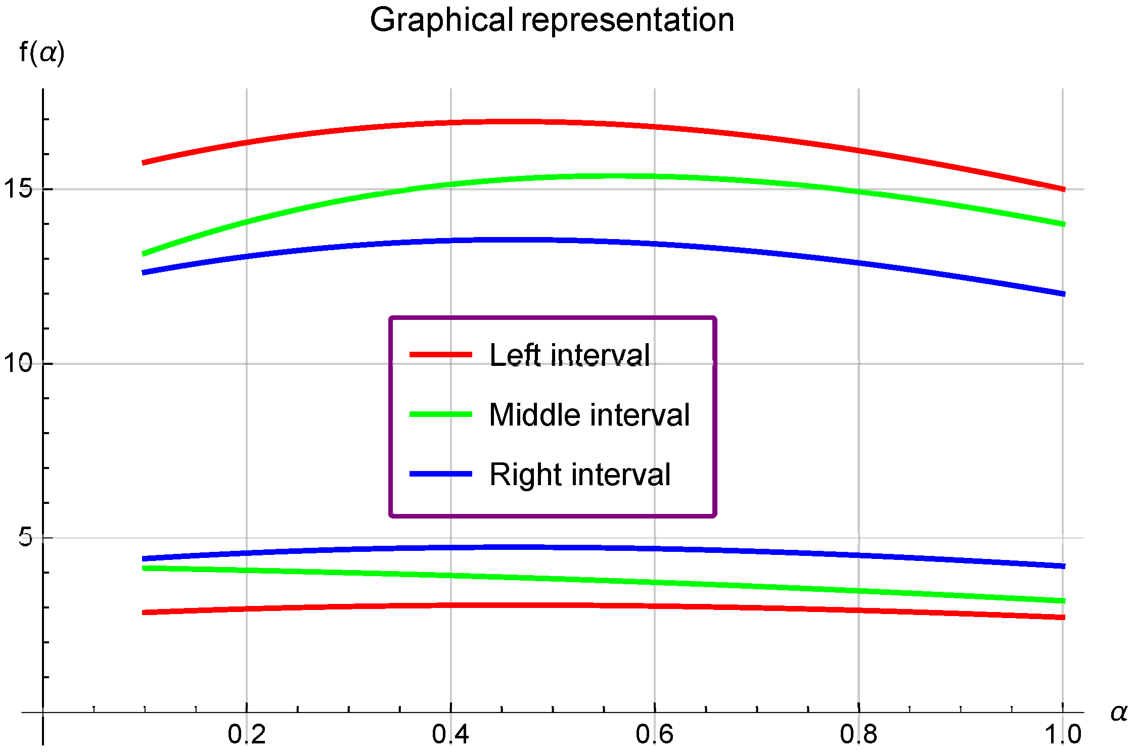
f v 1 + v 2 2 E μ , α + 1 , w , l γ , δ , k , c ( w ( v 2 v 1 ) μ ; p ) B ( α ) 2 α ( v 2 v 1 ) α ϵ μ , α , l , w , v 1 + γ , δ , k , c { f ( v 2 ; p ) } + ϵ μ , α , l , w , v 2 γ , δ , k , c { f ( v 1 ; p ) } ( 1 α ) B ( α ) ( f ( v 1 ) + f ( v 2 ) ) ( f ( v 1 ) + f ( v 2 ) ) 2 E μ , α + 1 , w , l γ , δ , k , c ( w ( v 2 v 1 ) μ ; p ) .
Example 1.
We set n = 0 , p = 0 , a n d α = 1 in Theorem 1. If f ( x ) = [ e x , 3 x 2 + 6 x + 12 ] and ζ ( v 2 , v 1 ) = v 2 v 1 , with v 1 = 0 and v 2 = 2 , then
f 2 v 1 + ζ ( v 2 , v 1 ) 2 E μ , α + 1 , w , l γ , δ , k , c ( w ( ζ ( v 2 , v 1 ) ) μ ; p ) = [ 2.72, 15 ] , B ( α ) 2 α ( ζ ( v 2 , v 1 ) ) α ϵ μ , α , l , w , v 1 + γ , δ , k , c { f ( v 1 + ζ ( v 2 , v 1 ) ; p ) } + ϵ μ , α , l , w , ( v 1 + ζ ( v 2 , v 1 ) ) γ , δ , k , c { f ( v 1 ; p ) } ( 1 α ) B ( α ) ( f ( v 1 ) + f ( v 1 + ζ ( v 2 , v 1 ) ) ) = 1 Γ ( α ) ( ζ 1 ( v 2 , v 1 ) ) α v 1 v 1 + ζ 1 ( v 1 , v 2 ) ( v 1 + ζ 1 ( v 1 , v 2 ) x ) α 1 f ( x ) d x + v 1 v 1 + ζ 1 ( v 1 , v 2 ) ( x v 1 ) α 1 f ( x ) d x = 1 2 α Γ ( α ) 0 2 ( 2 x ) α 1 [ 2 x 4 , 3 x 2 + 10 x + 2 ] d x + 0 2 ( x 0 ) α 1 [ 2 x 4 , 3 x 2 + 10 x + 2 ] d x = [ 3.19, 14 ] ( f ( v 1 ) + f ( v 1 + ζ ( v 2 , v 1 ) ) ) 2 E μ , α + 1 , w , l γ , δ , k , c ( w ( ζ ( v 2 , v 1 ) ) μ ; p ) = [ 4.19, 12 ] .
That implies that
[ 2.72, 15 ] [ 3.19, 14 ] [ 4.19, 12 ] .
Moreover, it gives the verification of Theorem 1.
  • If we choose n = 0 and p = 0 ζ ( v 2 , v 1 ) = v 2 v 1 , with v 1 = 0 , v 2 = 2 , α ( 0 , 1 ) , and f ( x ) = [ e x , 3 x 2 + 6 x + 12 ] in Theorem 1, then (see Figure 1).
Now, we derive a mid-point fractional analog of Hermite–Hadamard inequality.
Theorem 2.
Under the hypothesis considered in Theorem 1, the following inclusion relations hold true:
f 2 v 1 + ζ v 2 , v 1 2 E μ , α + 1 , w , l γ , δ , k , c w ζ v 2 , v 1 2 μ ; p 2 α 1 B ( α ) α ( ζ ( v 2 , v 1 ) ) α ϵ μ , α , l , w , 2 v 1 + ζ ( v 2 , v 1 ) 2 + γ , δ , k , c f ( v 1 + ζ ( v 2 , v 1 ) ; p ) + ϵ μ , α , l , w , 2 v 1 + ζ ( v 2 , v 1 ) 2 γ , δ , k , c { f ( v 1 ; p ) } ( 1 α ) B ( α ) ( f ( v 1 ) + f ( v 1 + ζ ( v 2 , v 1 ) ) ) f ( v 1 ) + f ( v 2 ) 2 E μ , α + 1 , w , l γ , δ , k , c ( w ( ζ ( v 2 , v 1 ) ) μ ; p ) .
Proof. 
In view of the interval-valued preinvexity of the function f, if we consider to take x = v 1 + 2 τ 2 ζ ( v 2 , v 1 ) and y = v 1 + τ 2 ζ ( v 2 , v 1 ) , as well as τ = 1 2 , then we know that
f 2 v 1 + ζ ( v 2 , v 1 ) 2 1 2 f v 1 + τ 2 ζ ( v 2 , v 1 ) + f v 1 + 2 τ 2 ζ ( v 2 , v 1 ) .
Multiplying both sides of (4) by ( τ 2 ) α 1 E μ , α , w , l γ , δ , k , c ( ( w ( ζ ( v 2 , v 1 ) ) μ ( τ 2 ) μ ; p ) and integrating the resulting inclusion with regard to τ on [ 0 , 1 ] , it yields that
f 2 v 1 + ζ ( v 2 , v 1 ) 2 0 1 τ 2 α 1 E μ , α , w , l γ , δ , k , c ( ( w ( ζ ( v 2 , v 1 ) ) μ τ 2 μ ; p ) d τ 1 2 0 1 τ 2 α 1 E μ , α , w , l γ , δ , k , c ( w ( ζ ( v 2 , v 1 ) ) μ τ 2 μ ; p ) f v 1 + τ 2 ζ ( v 2 , v 1 ) d τ + 0 1 τ 2 α 1 E μ , α , w , l γ , δ , k , c ( ( w ( ζ ( v 2 , v 1 ) ) μ τ 2 μ ; p ) f v 1 + 2 τ 2 ζ ( v 2 , v 1 ) d τ .
By means of the change in the variable and some calculations, we acquire that
f 2 v 1 + ζ ( v 2 , v 1 ) 2 E μ , α + 1 , w , l γ , δ , k , c w ζ v 2 , v 1 2 μ ; p 2 α 1 ( ζ ( v 2 , v 1 ) ) α 2 v 1 + ζ ( v 2 , v 1 ) 2 v 1 + ζ ( v 2 , v 1 ) ( v 1 + ζ ( v 2 , v 1 ) x ) α 1 E μ , α , w , l γ , δ , k , c ( w ( v 1 + ζ ( v 2 , v 1 ) x ) μ ; p ) d x + v 1 2 v 1 + ζ ( v 2 , v 1 ) 2 ( x v 1 ) α 1 E μ , α , w , l γ , δ , k , c ( w ( x v 1 ) μ ; p ) d x .
Hence,
f 2 v 1 + ζ ( v 2 , v 1 ) 2 E μ , α + 1 , w , l γ , δ , k , c w ζ v 2 , v 1 2 μ ; p 2 α 1 B ( α ) α ( ζ ( v 2 , v 1 ) ) α ϵ μ , α , l , w , 2 v 1 + ζ ( v 2 , v 1 ) 2 + γ , δ , k , c f ( v 1 + ζ ( v 2 , v 1 ) ; p ) + ϵ μ , α , l , w , 2 v 1 + ζ ( v 2 , v 1 ) 2 γ , δ , k , c { f ( v 1 ; p ) } ( 1 α ) B ( α ) ( f ( v 1 ) + f ( v 1 + ζ ( v 2 , v 1 ) ) ) .
Thich is the first inclusion relation.
For the proof of the second inequality, taking into account the interval-valued preinvexity of the function f, we know that
f v 1 + 2 τ 2 ζ ( v 2 , v 1 ) 1 2 [ τ f ( v 1 ) + ( 2 τ ) f ( v 2 ) ] ; f v 1 + τ 2 ζ ( v 2 , v 1 ) 1 2 [ ( 2 τ ) f ( v 1 ) + τ f ( v 2 ) ] .
Adding these relations above, we can deduce that
f v 1 + τ 2 ζ ( v 2 , v 1 ) + f v 1 + 2 τ 2 ζ ( v 2 , v 1 ) f ( v 1 ) + f ( v 2 )
Multiplying both sides of (5) by τ 2 α 1 E μ , α , w , l γ , δ , k , c ( ( w ( ζ ( v 2 , v 1 ) ) μ ( τ 2 ) μ ; p ) and integrating the resulting inclusion with regard to τ on [ 0 , 1 ] , it yields that
0 1 τ 2 α 1 E μ , α , w , l γ , δ , k , c ( ( w ( ζ ( v 2 , v 1 ) ) μ τ 2 μ ; p ) f v 1 + τ 2 ζ ( v 2 , v 1 ) d τ + 0 1 τ 2 α 1 E μ , α , w , l γ , δ , k , c ( ( w ( ζ ( v 2 , v 1 ) ) μ τ 2 μ ; p ) f v 1 + 2 τ 2 ζ ( v 2 , v 1 ) d τ [ f ( v 1 ) + f ( v 2 ) ] 0 1 τ 2 α 1 E μ , α , w , l γ , δ , k , c ( ( w ( ζ ( v 2 , v 1 ) ) μ τ 2 μ ; p ) d τ .
Changing variables, it yields that
2 α 1 B ( α ) α ( ζ ( v 2 , v 1 ) ) α ϵ μ , α , l , w , 2 v 1 + ζ ( v 2 , v 1 ) 2 + γ , δ , k , c f ( v 1 + ζ ( v 2 , v 1 ) ; p ) + ϵ μ , α , l , w , 2 v 1 + ζ ( v 2 , v 1 ) 2 γ , δ , k , c { f ( v 1 ; p ) } ( 1 α ) B ( α ) ( f ( v 1 ) + f ( v 1 + ζ ( v 2 , v 1 ) ) ) f ( v 1 ) + f ( v 2 ) 2 E μ , α + 1 , w , l γ , δ , k , c w ζ v 2 , v 1 2 μ ; p .
Thus, proof is accomplished. □
Special case
If we take ζ ( v 2 , v 1 ) = v 2 v 1 in Theorem 2, we acquire
f v 1 + v 2 2 E μ , α + 1 , w , l γ , δ , k , c w v 2 v 1 2 μ ; p 2 α 1 B ( α ) α ( v 2 v 1 ) α ϵ μ , α , l , w , v 1 + v 2 2 + γ , δ , k , c f ( v 2 ; p ) + ϵ μ , α , l , w , v 1 + v 2 2 γ , δ , k , c { f ( v 1 ; p ) } ( 1 α ) B ( α ) ( f ( v 1 ) + f ( v 2 ) ) f ( v 1 ) + f ( v 2 ) 2 E μ , α + 1 , w , l γ , δ , k , c w v 2 v 1 2 μ ; p .
Our next results are connected to Pachpatte-type inequalities.
Theorem 3.
Suppose that the two functions f , Ψ : [ v 1 , v 1 + ζ ( v 2 , v 1 ) ] R I + are both interval-valued preinvex and f ( x ) = [ f ̲ ( x ) , f ¯ ( x ) ] and Ψ ( x ) = [ g ̲ ( x ) , g ¯ ( x ) ] . Then, the successive inclusion relation holds true:
B ( α ) α ( ζ ( v 2 , v 1 ) ) α ϵ μ , α , l , w , v 1 + γ , δ , k , c { f ( v 1 + ζ ( v 2 , v 1 ) ; p ) Ψ ( v 1 + ζ ( v 2 , v 1 ) ; p ) } + ϵ μ , α , l , w , ( v 1 + ζ ( v 2 , v 1 ) ) γ , δ , k , c { f ( v 1 ; p ) Ψ ( v 1 ; p ) } ( 1 α ) B ( α ) ( f ( v 1 ) Ψ ( v 1 ) + f ( v 1 + ζ ( v 2 , v 1 ) ) Ψ ( v 1 + ζ ( v 2 , v 1 ) ) ) 2 E 0 [ P ( v 1 , v 2 ) + Q ( v 1 , v 2 ) ] + P ( v 1 , v 2 ) E μ , α + 1 , w , l γ , δ , k , c ( w ( ζ ( v 2 , v 1 ) ) μ ; p ) ,
where
P ( v 1 , v 2 ) : = f ( v 1 ) Ψ ( v 1 ) + f ( v 2 ) Ψ ( v 2 ) , Q ( v 1 , v 2 ) : = f ( v 1 ) Ψ ( v 2 ) + f ( v 2 ) Ψ ( v 1 ) , E 0 : = n = 0 β p ( γ + n k , c γ ) β ( γ , c γ ) ( c ) n k ( μ n + α + 1 ) ( μ n + α + 2 ) Γ ( μ n + α ) τ n ( l ) n δ .
Proof. 
Applying the preinvexity of the interval-valued functions f and Ψ , we have
f ( v 1 + τ ζ ( v 2 , v 1 ) ) τ f ( v 1 ) + ( 1 τ ) f ( v 2 ) ,
and
Ψ ( v 1 + τ ζ ( v 2 , v 1 ) ) τ Ψ ( v 1 ) + ( 1 τ ) Ψ ( v 2 ) ,
Multiplying (7) and (8), we obtain
f ( v 1 + τ ζ ( v 2 , v 1 ) ) Ψ ( v 1 + τ ζ ( v 2 , v 1 ) ) τ 2 f ( v 1 ) Ψ ( v 1 ) + ( 1 τ ) 2 f ( v 2 ) Ψ ( v 2 ) + τ ( 1 τ ) [ f ( v 1 ) Ψ ( v 2 ) + f ( v 2 ) Ψ ( v 1 ) ]
Similarly, we have
f ( v 1 + ( 1 τ ) ζ ( v 2 , v 1 ) ) Ψ ( v 1 + ( 1 τ ) ζ ( v 2 , v 1 ) ) ( 1 τ ) 2 f ( v 1 ) Ψ ( v 1 ) + τ 2 f ( v 2 ) Ψ ( v 2 ) + τ ( 1 τ ) [ f ( v 1 ) Ψ ( v 2 ) + f ( v 2 ) Ψ ( v 1 ) ]
Adding (9) and (10), we obtain
f ( v 1 + τ ζ ( v 2 , v 1 ) ) Ψ ( v 1 + τ ζ ( v 2 , v 1 ) ) + f ( v 1 + ( 1 τ ) ζ ( v 2 , v 1 ) ) Ψ ( v 1 + ( 1 τ ) ζ ( v 2 , v 1 ) ) [ τ 2 + ( 1 τ ) 2 ] [ f ( v 1 ) Ψ ( v 1 ) + f ( v 2 ) Ψ ( v 2 ) ] + 2 τ ( 1 τ ) [ f ( v 1 ) Ψ ( v 2 ) + f ( v 2 ) Ψ ( v 1 ) ] = ( 2 τ 2 2 τ + 1 ) P ( v 1 , v 2 ) + ( 2 τ 2 + 2 τ ) Q ( v 1 , v 2 )
Multiplying both sides by τ α 1 E μ , α , w , l γ , δ , k , c ( ( w ( ζ ( v 2 , v 1 ) ) μ τ μ ; p ) and integrating the resulting inclusion with regard to τ on [ 0 , 1 ] , we have
0 1 τ α 1 E μ , α , w , l γ , δ , k , c ( ( w ( ζ ( v 2 , v 1 ) ) μ τ μ ; p ) f ( v 1 + τ ζ ( v 2 , v 1 ) ) Ψ ( v 1 + τ ζ ( v 2 , v 1 ) ) d τ + 0 1 τ α 1 E μ , α , w , l γ , δ , k , c ( ( w ( ζ ( v 2 , v 1 ) ) μ τ μ ; p ) f ( v 1 + ( 1 τ ) ζ ( v 2 , v 1 ) ) Ψ ( v 1 + ( 1 τ ) ζ ( v 2 , v 1 ) ) d τ P ( v 1 , v 2 ) 0 1 τ α 1 E μ , α , w , l γ , δ , k , c ( ( w ( ζ ( v 2 , v 1 ) ) μ τ μ ; p ) ( 2 τ 2 2 τ + 1 ) d τ + Q ( v 1 , v 2 ) 0 1 τ α 1 E μ , α , w , l γ , δ , k , c ( ( w ( ζ ( v 2 , v 1 ) ) μ τ μ ; p ) ( 2 τ 2 + 2 τ ) d τ
By means of changes in variables and simple calculation, we obtained the required result. □
Special case
If we take ζ ( v 2 , v 1 ) = v 2 v 1 in Theorem 3, we obtain the result for the interval-valued convex function.
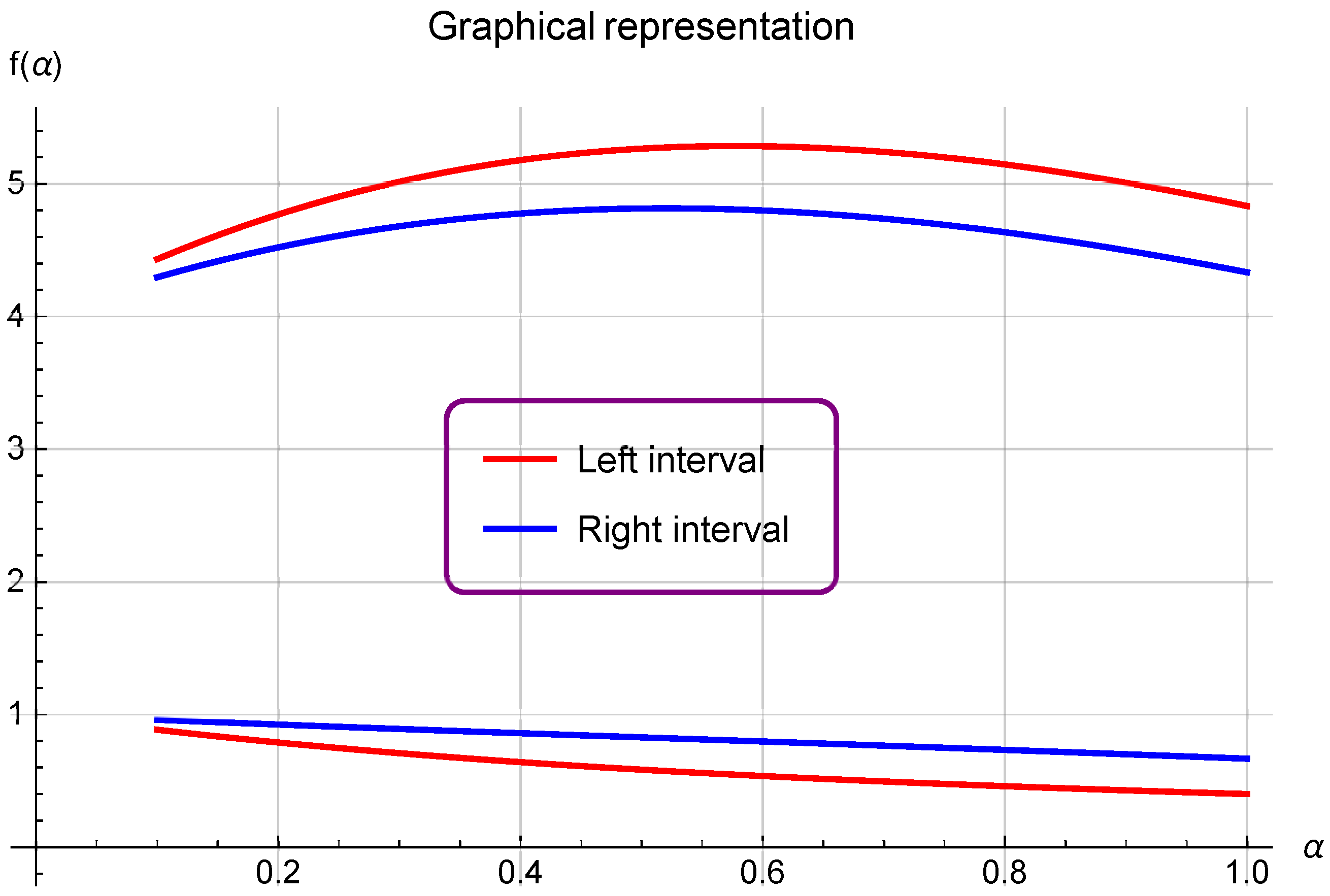
B ( α ) α ( v 2 v 1 ) α ϵ μ , α , l , w , v 1 + γ , δ , k , c { f ( v 2 ; p ) Ψ ( v 2 ; p ) } + ϵ μ , α , l , w , v 2 γ , δ , k , c { f ( v 1 ; p ) Ψ ( v 1 ; p ) } ( 1 α ) B ( α ) ( f ( v 1 ) Ψ ( v 1 ) + f ( v 2 ) Ψ ( v 2 ) ) 2 E 0 [ P ( v 1 , v 2 ) + Q ( v 1 , v 2 ) ] + P ( v 1 , v 2 ) E μ , α + 1 , w , l γ , δ , k , c ( w ( v 2 v 1 ) μ ; p ) ,
Example 2.
We set n = 0 , p = 0 , and α = 1 in Theorem 3. If f ( x ) = [ x 2 , 2 x 2 ] and Ψ ( x ) = [ x 2 , x + 1 ] and ζ ( v 2 , v 1 ) = v 2 v 1 , with v 1 = 0 and v 2 = 1 , then
B ( α ) α ( ζ ( v 2 , v 1 ) ) α ϵ μ , α , l , w , v 1 + γ , δ , k , c { f ( v 1 + ζ ( v 2 , v 1 ) ; p ) Ψ ( v 1 + ζ ( v 2 , v 1 ) ; p ) } + ϵ μ , α , l , w , ( v 1 + ζ ( v 2 , v 1 ) ) γ , δ , k , c { f ( v 1 ; p ) Ψ ( v 1 ; p ) } ( 1 α ) B ( α ) ( f ( v 1 ) Ψ ( v 1 ) + f ( v 1 + ζ ( v 2 , v 1 ) ) Ψ ( v 1 + ζ ( v 2 , v 1 ) ) ) = [ 0.4, 4.84] P ( v 1 , v 2 ) = f ( v 1 ) Ψ ( v 1 ) + f ( v 2 ) Ψ ( v 2 ) = [ 1 , 4 ] , Q ( v 1 , v 2 ) = f ( v 1 ) Ψ ( v 2 ) + f ( v 2 ) Ψ ( v 1 ) = [ 0 , 5 ] .
That implies that
[ 0.4, 4.84] [ 0.67, 4.33]
which gives the verification of Theorem 3.
  • If we choose n = 0 , p = 0 , and ζ ( v 2 , v 1 ) = v 2 v 1 , with v 1 = 0 , v 2 = 2 , α ( 0 , 1 ) , f ( x ) = [ x 2 , 2 x 2 ] , and Ψ ( x ) = [ x 2 , x + 1 ] in Theorem 3, then (see Figure 2).
Figure 2. This is an image showing the comparison between left and right sides of Theorem 3.
Symmetry 15 01012 g002
Theorem 4.
Under the same hypothesis mentioned in Theorem 3, the following successive inclusion relation holds true:
f 2 v 1 + ζ ( v 2 , v 1 ) 2 Ψ 2 v 1 + ζ ( v 2 , v 1 ) 2 E μ , α + 1 , w , l γ , δ , k , c ( w ( ζ ( v 2 , v 1 ) ) μ ; p ) B ( α ) 4 α ( ζ ( v 2 , v 1 ) ) α ϵ μ , α , l , w , v 1 + γ , δ , k , c { f ( v 1 + ζ ( v 2 , v 1 ) ; p ) Ψ ( v 1 + ζ ( v 2 , v 1 ) ; p ) } + ϵ μ , α , l , w , ( v 1 + ζ ( v 2 , v 1 ) ) γ , δ , k , c { f ( v 1 ; p ) Ψ ( v 1 ; p ) } ( 1 α ) B ( α ) ( f ( v 1 ) Ψ ( v 1 ) + f ( v 1 + ζ ( v 2 , v 1 ) ) Ψ ( v 1 + ζ ( v 2 , v 1 ) ) ) + 1 2 E 0 [ P ( v 1 , v 2 ) Q ( v 1 , v 2 ) ] + 1 4 Q ( v 1 , v 2 ) E μ , α + 1 , w , l γ , δ , k , c ( w ( ζ ( v 2 , v 1 ) ) μ ; p ) .
Proof. 
For τ [ 0 , 1 ] , we have
2 v 1 + ζ ( v 2 , v 1 ) 2 = v 1 + τ ζ ( v 2 , v 1 ) 2 + v 1 + ( 1 τ ) ζ ( v 2 , v 1 ) 2 .
Since f and Ψ are non-negative interval-valued preinvex functions, we have
f 2 v 1 + ζ ( v 2 , v 1 ) 2 Ψ 2 v 1 + ζ ( v 2 , v 1 ) 2 = f v 1 + τ ζ ( v 2 , v 1 ) 2 + v 1 + ( 1 τ ) ζ ( v 2 , v 1 ) 2 × Ψ v 1 + τ ζ ( v 2 , v 1 ) 2 + v 1 + ( 1 τ ) ζ ( v 2 , v 1 ) 2 1 4 [ f ( v 1 + τ ζ ( v 2 , v 1 ) ) + f ( v 1 + ( 1 τ ) ζ ( v 2 , v 1 ) ) ] [ Ψ ( v 1 + τ ζ ( v 2 , v 1 ) ) + Ψ ( v 1 + ( 1 τ ) ζ ( v 2 , v 1 ) ) ] = 1 4 [ f ( v 1 + τ ζ ( v 2 , v 1 ) ) Ψ ( v 1 + τ ζ ( v 2 , v 1 ) ) + f ( v 1 + ( 1 τ ) ζ ( v 2 , v 1 ) ) Ψ ( v 1 + τ ζ ( v 2 , v 1 ) ) + f ( v 1 + τ ζ ( v 2 , v 1 ) ) Ψ ( v 1 + ( 1 τ ) ζ ( v 2 , v 1 ) ) + f ( v 1 + ( 1 τ ) ζ ( v 2 , v 1 ) ) Ψ ( v 1 + ( 1 τ ) ζ ( v 2 , v 1 ) ) ] 1 4 [ f ( v 1 + τ ζ ( v 2 , v 1 ) ) Ψ ( v 1 + τ ζ ( v 2 , v 1 ) ) + f ( v 1 + ( 1 τ ) ζ ( v 2 , v 1 ) ) Ψ ( v 1 + ( 1 τ ) ζ ( v 2 , v 1 ) ) ] 1 4 [ ( 2 τ 2 + 2 τ ) P ( v 1 , v 2 ) + ( 2 τ 2 2 τ + 1 ) Q ( v 1 , v 2 ) ] .
Multiplying both sides by τ α 1 E μ , α , w , l γ , δ , k , c ( ( w ( ζ ( v 2 , v 1 ) ) μ τ μ ; p ) and integrating the resulting inclusion with regard to τ on [ 0 , 1 ] , we have
f 2 v 1 + ζ ( v 2 , v 1 ) 2 Ψ 2 v 1 + ζ ( v 2 , v 1 ) 2 0 1 τ α 1 E μ , α , w , l γ , δ , k , c ( ( w ( ζ ( v 2 , v 1 ) ) μ τ μ ; p ) d τ 1 4 0 1 τ α 1 E μ , α , w , l γ , δ , k , c ( ( w ( ζ ( v 2 , v 1 ) ) μ τ μ ; p ) f ( v 1 + τ ζ ( v 2 , v 1 ) ) Ψ ( v 1 + τ ζ ( v 2 , v 1 ) ) d τ + 1 4 0 1 τ α 1 E μ , α , w , l γ , δ , k , c ( ( w ( ζ ( v 2 , v 1 ) ) μ τ μ ; p ) f ( v 1 + ( 1 τ ) ζ ( v 2 , v 1 ) ) Ψ ( v 1 + ( 1 τ ) ζ ( v 2 , v 1 ) ) d τ + 1 4 P ( v 1 , v 2 ) 0 1 τ α 1 E μ , α , w , l γ , δ , k , c ( ( w ( ζ ( v 2 , v 1 ) ) μ τ μ ; p ) ( 2 τ 2 + 2 τ ) d τ + 1 4 Q ( v 1 , v 2 ) 0 1 τ α 1 E μ , α , w , l γ , δ , k , c ( ( w ( ζ ( v 2 , v 1 ) ) μ τ μ ; p ) ( 2 τ 2 2 τ + 1 ) d τ .
By means of changes in variables and some calculations, we obtained the required result. □
Special case
If we take ζ ( v 2 , v 1 ) = v 2 v 1 in Theorem 4, we obtain the result for the interval-valued convex function.
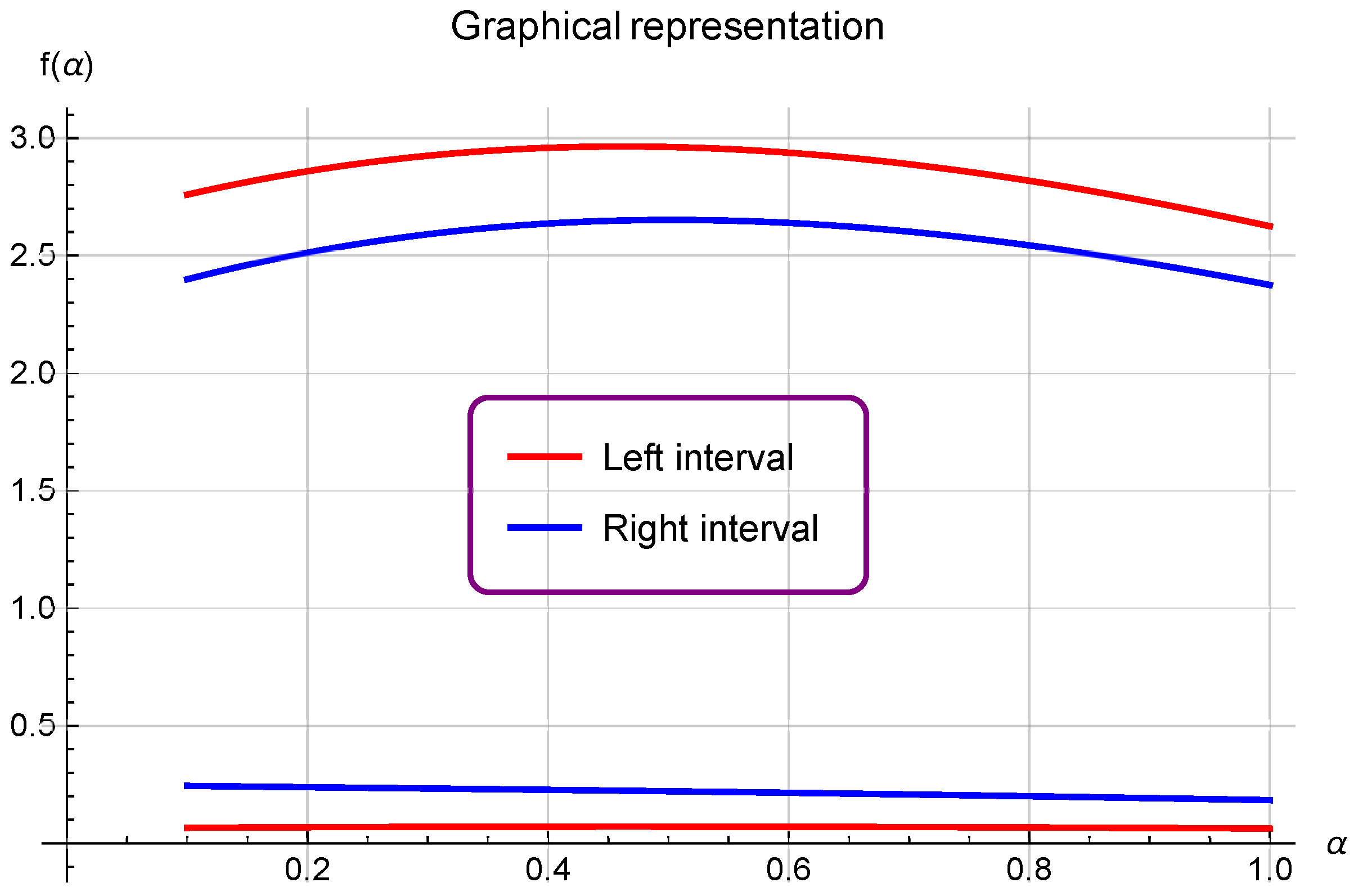
f v 1 + v 2 2 Ψ v 1 + v 2 2 E μ , α + 1 , w , l γ , δ , k , c ( w ( v 2 v 1 ) μ ; p ) B ( α ) 4 α ( v 2 v 1 ) α ϵ μ , α , l , w , v 1 + γ , δ , k , c { f ( v 2 ; p ) Ψ ( v 2 ; p ) } + ϵ μ , α , l , w , v 2 γ , δ , k , c { f ( v 1 ; p ) Ψ ( v 1 ; p ) } ( 1 α ) B ( α ) ( f ( v 1 ) Ψ ( v 1 ) + f ( v 2 ) Ψ ( v 2 ) + 1 2 E 0 [ P ( v 1 , v 2 ) Q ( v 1 , v 2 ) ] + 1 4 Q ( v 1 , v 2 ) E μ , α + 1 , w , l γ , δ , k , c ( w ( v 2 v 1 ) μ ; p ) .
Example 3.
We set n = 0 , p = 0 , a n d α = 1 in Theorem 4. If f ( x ) = [ x 2 , 2 x 2 ] and Ψ ( x ) = [ x 2 , x + 1 ] and ζ ( v 2 , v 1 ) = v 2 v 1 , with v 1 = 0 and v 2 = 1 , then
f 2 v 1 + ζ ( v 2 , v 1 ) 2 Ψ 2 v 1 + ζ ( v 2 , v 1 ) 2 E μ , α + 1 , w , l γ , δ , k , c ( w ( ζ ( v 2 , v 1 ) ) μ ; p ) = [ 0.0625, 2.625] , B ( α ) 4 α ( ζ ( v 2 , v 1 ) ) α ϵ μ , α , l , w , v 1 + γ , δ , k , c { f ( v 1 + ζ ( v 2 , v 1 ) ; p ) Ψ ( v 1 + ζ ( v 2 , v 1 ) ; p ) } + ϵ μ , α , l , w , ( v 1 + ζ ( v 2 , v 1 ) ) γ , δ , k , c { f ( v 1 ; p ) Ψ ( v 1 ; p ) } ( 1 α ) B ( α ) ( f ( v 1 ) Ψ ( v 1 ) + f ( v 1 + ζ ( v 2 , v 1 ) ) Ψ ( v 1 + ζ ( v 2 , v 1 ) ) ) + 1 2 E 0 [ P ( v 1 , v 2 ) Q ( v 1 , v 2 ) ] + 1 4 Q ( v 1 , v 2 ) E μ , α + 1 , w , l γ , δ , k , c ( w ( ζ ( v 2 , v 1 ) ) μ ; p ) = [ 0.183, 2.377] P ( v 1 , v 2 ) = f ( v 1 ) Ψ ( v 1 ) + f ( v 2 ) Ψ ( v 2 ) = [ 1 , 4 ] , Q ( v 1 , v 2 ) = f ( v 1 ) Ψ ( v 2 ) + f ( v 2 ) Ψ ( v 1 ) = [ 0 , 5 ] .
That implies that
[ 0.0625, 2.625] [ 0.183, 2.377]
which gives the verification of Theorem 4.
  • If we choose n = 0 and p = 0 , ζ ( v 2 , v 1 ) = v 2 v 1 , with v 1 = 0 , v 2 = 2 , α ( 0 , 1 ) , f ( x ) = [ x 2 , 2 x 2 ] , and Ψ ( x ) = [ x 2 , x + 1 ] in Theorem 4, then (see Figure 3).
Finally, we investigate new fractional Hermite–Hadamard–Fejer-type inclusions for interval-valued preinvex functions.
Theorem 5.
Suppose that f : K R R I + is a given interval-valued preinvex function defined over [ v 1 , v 1 + ζ ( v 2 , v 1 ) ] together with 0 v 1 < v 1 + ζ ( v 2 , v 1 ) , and f ( x ) = [ f ̲ ( x ) , f ¯ ( x ) ] . If the function Φ : [ v 1 , v 1 + ζ ( v 2 , v 1 ) ] R R is non-negative-integrable and symmetric with respect to 2 v 1 + ζ ( v 2 , v 1 ) 2 , i.e., Φ ( 2 v 1 + ζ ( v 2 , v 1 ) x ) = Φ ( x ) , then we have
f 2 v 1 + ζ ( v 2 , v 1 ) 2 ϵ μ , α , l , w , v 1 + γ , δ , k , c { Φ ( v 1 + ζ ( v 2 , v 1 ) ; p ) } + ϵ μ , α , l , w , ( v 1 + ζ ( v 2 , v 1 ) ) γ , δ , k , c { Φ ( v 1 ) ; p ) } ( 1 α ) B ( α ) ( Φ ( v 1 + ζ ( v 2 , v 1 ) ) + Φ ( v 1 ) ) ϵ μ , α , l , w , v 1 + γ , δ , k , c { f ( v 1 + ζ ( v 2 , v 1 ) ; p ) Φ ( v 1 + ζ ( v 2 , v 1 ) ; p ) } + ϵ μ , α , l , w , ( v 1 + ζ ( v 2 , v 1 ) ) γ , δ , k , c { f ( v 1 ; p ) Φ ( v 1 ; p ) } ( 1 α ) B ( α ) ( f ( v 1 + ζ ( v 2 , v 1 ) ) Φ ( v 1 + ζ ( v 2 , v 1 ) ) + f ( v 1 ) Φ ( v 1 ) ) f ( v 1 ) + f ( v 2 ) 2 ϵ μ , α , l , w , v 1 + γ , δ , k , c { Φ ( v 1 + ζ ( v 2 , v 1 ) ; p ) } + ϵ μ , α , l , w , ( v 1 + ζ ( v 2 , v 1 ) ) γ , δ , k , c { Φ ( v 1 ; p ) } ( 1 α ) B ( α ) ( Φ ( v 1 ) + Φ ( v 1 + ζ ( v 2 , v 1 ) ) ) .
Proof. 
Proceeding from the relation (2) within the proof of Theorem 1, multiplying both sides of it with 2 τ α 1 E μ , α , w , l γ , δ , k , c ( ( w ( ζ ( v 2 , v 1 ) ) μ τ μ ; p ) Φ ( v 1 + τ ζ ( v 2 , v 1 ) ) and integrating the resulting inclusion with regard to τ on [ 0 , 1 ] , we derive that
2 f 2 v 1 + ζ ( v 2 , v 1 ) 2 0 1 τ α 1 E μ , α , w , l γ , δ , k , c ( ( w ( ζ ( v 2 , v 1 ) ) μ τ μ ; p ) Φ ( v 1 + τ ζ ( v 2 , v 1 ) ) d τ 2 2 0 1 τ α 1 E μ , α , w , l γ , δ , k , c ( w ( ζ ( v 2 , v 1 ) ) μ τ μ ; p ) Φ ( v 1 + τ ζ ( v 2 , v 1 ) ) f ( v 1 + τ ζ ( v 2 , v 1 ) ) d τ + 0 1 0 1 τ α 1 s β 1 E μ , α , w , l γ , δ , k , c ( ( w ( ζ ( v 2 , v 1 ) ) μ τ μ ; p ) Φ ( v 1 + τ ζ ( v 2 , v 1 ) ) f ( v 1 + ( 1 τ ) ζ ( v 2 , v 1 ) ) d τ .
Taking into consideration the change in the variable, we acquire that
2 f 2 v 1 + ζ ( v 2 , v 1 ) 2 ( ζ ( v 2 , v 1 ) ) α v 1 v 1 + ζ ( v 2 , v 1 ) ( v 1 + ζ ( v 2 , v 1 ) x ) α 1 E μ , α , w , l γ , δ , k , c ( ( w ( v 1 + ζ ( v 2 , v 1 ) x ) μ ; p ) Φ ( x ) d x 1 ( ζ ( v 2 , v 1 ) ) α v 1 v 1 + ζ ( v 2 , v 1 ) ( v 1 + ζ ( v 2 , v 1 ) x ) α 1 E μ , α , w , l γ , δ , k , c ( w ( v 1 + ζ ( v 2 , v 1 ) x ) μ ; p ) f ( x ) Φ ( x ) d x + v 1 v 1 + ζ ( v 2 , v 1 ) ( x v 1 ) α 1 E μ , α , w , l γ , δ , k , c ( w ( x v 1 ) μ ; p ) f ( x ) Φ ( x ) d x .
In accordance with the symmetry of the function Φ ( x ) , it yields that
B ( α ) f 2 v 1 + ζ ( v 2 , v 1 ) 2 α β ( ζ ( v 2 , v 1 ) ) α ϵ μ , α , l , w , v 1 + γ , δ , k , c { Φ ( v 1 + ζ ( v 2 , v 1 ) ; p ) } + ϵ μ , α , l , w , ( v 1 + ζ ( v 2 , v 1 ) ) γ , δ , k , c { Φ ( v 1 ; p ) } ( 1 α ) B ( α ) ( Φ ( v 1 + ζ ( v 2 , v 1 ) + Φ ( v 1 ) ) B ( α ) α ( ζ ( v 2 , v 1 ) ) α ϵ μ , α , l , w , v 1 + γ , δ , k , c { f ( v 1 + ζ ( v 2 , v 1 ) ; p ) Φ ( v 1 + ζ ( v 2 , v 1 ) } + ϵ μ , α , l , w , ( v 1 + ζ ( v 2 , v 1 ) ) γ , δ , k , c { f ( v 1 ; p ) Φ ( v 1 ; p ) } ( 1 α ) B ( α ) ( f ( v 1 + ζ ( v 2 , v 1 ) ) Φ ( v 1 + ζ ( v 2 , v 1 ) ) + f ( v 1 ) Φ ( v 1 ) ) .
This ends the proof of the first inclusion relation.
To establish the second inclusion relation, we will build upon inclusion relation (3) from the proof of Theorem 1. We begin by multiplying both sides of (3) with τ α 1 E μ , α , w , l γ , δ , k , c ( w ( ζ ( v 2 , v 1 ) ) μ τ μ ; p ) Φ ( v 1 + τ ζ ( v 2 , v 1 ) ) . Then, we integrate the resulting inclusion with respect to τ over the interval [ 0 , 1 ] , leading to the following conclusion:
0 1 τ α 1 E μ , α , w , l γ , δ , k , c ( w ( ζ ( v 2 , v 1 ) ) μ τ μ ; p ) Φ ( v 1 + τ ζ ( v 2 , v 1 ) ) [ f ( v 1 + τ ζ ( v 2 , v 1 ) ) + f ( v 1 + ( 1 τ ) ζ ( v 2 , v 1 ) ) ] d τ [ f ( v 1 ) + f ( v 2 ) ] 0 1 τ α 1 E μ , α , w , l γ , δ , k , c ( w ( ζ ( v 2 , v 1 ) ) μ τ μ ; p ) Φ ( v 1 + τ ζ ( v 2 , v 1 ) ) d s d τ .
Changing variables, it yields that
ϵ μ , α , l , w , v 1 + γ , δ , k , c { f ( v 1 + ζ ( v 2 , v 1 ) ; p ) Φ ( v 1 + ζ ( v 2 , v 1 ) ; p ) } + ϵ μ , α , l , w , ( v 1 + ζ ( v 2 , v 1 ) ) γ , δ , k , c { f ( v 1 ; p ) Φ ( v 1 ; p ) } ( 1 α ) B ( α ) ( f ( v 1 + ζ ( v 2 , v 1 ) ) Φ ( v 1 + ζ ( v 2 , v 1 ) ) + f ( v 1 ) Φ ( v 1 ) ) f ( v 1 ) + f ( v 2 ) 2 ϵ μ , α , l , w , v 1 + γ , δ , k , c { Φ ( v 1 + ζ ( v 2 , v 1 ) ; p ) } + ϵ μ , α , l , w , ( v 1 + ζ ( v 2 , v 1 ) ) γ , δ , k , c { Φ ( v 1 ; p ) } ( 1 α ) B ( α ) ( Φ ( v 1 ) + Φ ( v 1 + ζ ( v 2 , v 1 ) ) ) .
Thus, the proof is completed. □
Special case
If we take ζ ( v 2 , v 1 ) = v 2 v 1 in Theorem 5, we obtain the result for the interval-valued convex function.
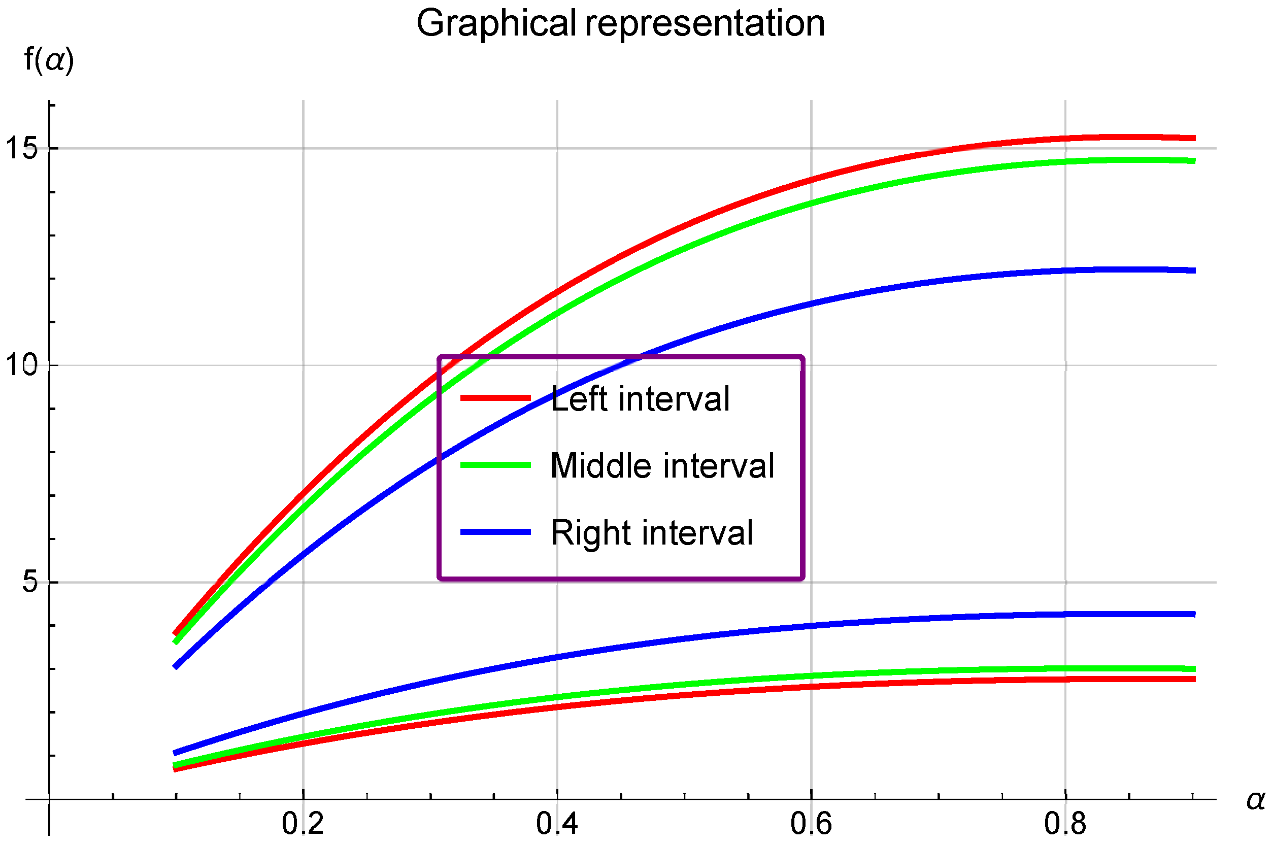
f v 1 + v 2 2 ϵ μ , α , l , w , v 1 + γ , δ , k , c { Φ ( v 2 ; p ) } + ϵ μ , α , l , w , v 2 γ , δ , k , c { Φ ( v 1 ) ; p ) } ( 1 α ) B ( α ) ( Φ ( v 2 ) + Φ ( v 1 ) ) ϵ μ , α , l , w , v 1 + γ , δ , k , c { f ( v 2 ; p ) Φ ( v 2 ; p ) } + ϵ μ , α , l , w , v 2 γ , δ , k , c { f ( v 1 ; p ) Φ ( v 1 ; p ) } ( 1 α ) B ( α ) ( f ( v 2 ) Φ ( v 2 ) + f ( v 1 ) Φ ( v 1 ) ) f ( v 1 ) + f ( v 2 ) 2 ϵ μ , α , l , w , v 1 + γ , δ , k , c { Φ ( v 2 ; p ) } + ϵ μ , α , l , w , v 2 γ , δ , k , c { Φ ( v 1 ; p ) } ( 1 α ) B ( α ) ( Φ ( v 1 ) + Φ ( v 2 ) ) .
Example 4.
We set n = 0 , p = 0 , and α = 1 in Theorem 5. If f ( x ) = [ e x 2 , 3 x 2 + 6 x + 12 ] and
Φ ( x ) = x , x [ 0 , 1 ] x + 2 , x [ 0 , 1 ] .
and ζ ( v 2 , v 1 ) = v 2 v 1 , with v 1 = 0 and v 2 = 2 , then
f v 1 + v 2 2 2 0 2 Φ ( x ) d x = [ 5.44, 30 ] 2 0 2 f ( x ) Φ ( x ) d x = [ 5.9, 29 ] f ( v 1 ) + f ( v 2 ) 2 2 0 2 Φ ( x ) d x = [ 8.39, 24 ] .
That implies that
[ 5.44, 30 ] [ 5.9, 29 ] [ 8.39, 24 ]
which gives the verification of Theorem 5.
  • If we choose n = 0 , p = 0 , and ζ ( v 2 , v 1 ) = v 2 v 1 , with v 1 = 0 , v 2 = 2 , α ( 0 , 1 ) , and f ( x ) = [ e x 2 , 3 x 2 + 6 x + 12 ] in Theorem 5, then (see Figure 4).

3. Conclusions

In recent years, the theory of inequality has expanded at a very fast rate considering the convexity characteristics of the functions specifically in fractional domains. Several new operators have been introduced incorporating the nonsingular kernels. By making use of these operators, several fractional variants of renowned integral inequalities have been established in the literature. Motivated by these kinds of aspects, we have devised a new family of fractional operators involving generalized Mittag-Leffler functions, consisting of seven parameters in the Ab sense. This paper has introduced novel Hermite–Hadamard-, Hermite–Hadamard–Fejer-, and Pachpatte-type inclusions in the fractional setting utilizing extended Mittag-Leffler functions as a kernel. Additionally, special cases and numerical examples have been presented. Going forward, our future research aims to derive new fuzzy variants of Hermite–Hadamard-type inequalities and Hermite–Hadamard–Mercer-type inequalities using newly developed integral operators and higher-order convexity. We hope that our work will spark the interest of readers and encourage further research in this area.

Author Contributions

Conceptualization, M.Z.J., M.U.A. and M.A.N.; methodology, M.U.A.; software, B.B.-M. and M.Z.J.; validation, M.U.A., M.V.M. and H.B.; formal analysis, M.Z.J., M.U.A., M.V.M., H.B. and A.G.K.; investigation, M.Z.J., M.U.A., M.V.M. and H.B.; writing—original draft preparation, B.B.-M., M.Z.J., M.U.A., M.V.M., H.B., A.G.K. and M.A.N.; writing—review and editing, M.Z.J. and M.U.A. supervision, M.U.A. All authors have read and agreed to the published version of the manuscript.

Funding

This Research is supported by Researchers Supporting Project number (RSP2023R158), King Saud University, Riyadh, Saudi Arabia.

Data Availability Statement

No data were used to support this study.

Acknowledgments

The authors are thankful to the editor and the anonymous reviewers for their valuable comments and suggestions.

Conflicts of Interest

The authors declare that they have no conflict of interest.

References

  1. Dragomir, S.S.; Pearce, C.E.M. Selected Topics on Hermite-Hadamard Inequalities and Applications; RGMIA Victoria University: Melbourne, Australia, 2000. [Google Scholar]
  2. Cerone, P.; Dragomir, S.S. On some inequalities for the expectation and variance. Korean J. Comput. Appl. Math. 2000, 2, 357–380. [Google Scholar] [CrossRef] [Green Version]
  3. Pečarič, J.E.; Proschan, F.; Tong, Y.L. Convex Functions, Partial Ordering and Statistical Applications; Academic Press: New York, NY, USA, 1991. [Google Scholar]
  4. Weir, T.; Mond, B. Preinvex functions in multiple objective optimization. J. Math. Anal. Appl. 1988, 136, 29–38. [Google Scholar] [CrossRef] [Green Version]
  5. Mohan, M.S.; Neogy, S.K. On invex sets and preinvex functions. J. Math. Anal. Appl. 1995, 189, 901–908. [Google Scholar] [CrossRef] [Green Version]
  6. Breckner, W.W. Continuity of generalized convex and generalized concave set-valued functions. Rev. D’Anal. Numer. Theor. L’Approx. 1993, 22, 39–51. [Google Scholar]
  7. Sharma, N.; Singh, S.K.; Mishra, S.K.; Hamdi, A. Hermite-Hadamard-type inequalities for interval-valued preinvex functions via Riemann-Liouville fractional integrals. J. Inequalities Appl. 2021, 2021, 98. [Google Scholar] [CrossRef]
  8. Farid, G.; Akbar, S.B.; Rehman, S.U.; Pecaric, J. Boundedness of fractional integral operators containing Mittag-Leffler functions via (s,m)-convexity. Aims Math. 2020, 5, 966–978. [Google Scholar] [CrossRef]
  9. Atangana, A.; Baleanu, D. New Fractional Derivatives with Non-Local and Non-Singular Kernel: Theory and Application to Heat Transfer Model. Therm. Sci. 2016, 20, 763–769. [Google Scholar] [CrossRef] [Green Version]
  10. Du, T.; Zhou, T. On the fractional double integral inclusion relations having exponential kernels via interval-valued co-ordinated convex mappings. Chaos Solitons Fractals 2022, 156, 111846. [Google Scholar] [CrossRef]
  11. Sarikaya, M.Z.; Set, E.; Yaldiz, H.; Basak, N. Hermite-Hadamard’s inequalities for fractional integrals and related fractional inequalities. Math. Comput. Model. 2013, 57, 2403–2407. [Google Scholar] [CrossRef]
  12. Mohammed, P.O.; Sarikaya, M.Z.; Baleanu, D. On the generalized Hermite-Hadamard inequalities via the tempered fractional integrals. Symmetry 2020, 12, 595. [Google Scholar] [CrossRef] [Green Version]
  13. Mohammed, P.O.; Brevik, I. A new version of the Hermite-Hadamard inequality for Riemann-Liouville fractional integrals. Symmetry 2020, 12, 610. [Google Scholar] [CrossRef] [Green Version]
  14. Akdemir, A.O.; Butt, S.I.; Nadeem, M.; Ragusa, M.A. New general variants of Chebyshev type inequalities via generalized fractional integral operators. Mathematics 2021, 9, 122. [Google Scholar] [CrossRef]
  15. Set, E.; Butt, S.I.; Akdemir, A.O.; Karaoglan, A.; Abdeljawad, T. New integral inequalities for differentiable convex functions via Atangana-Baleanu fractional integral operators. Chaos Solitons Fractals 2021, 143, 110554. [Google Scholar] [CrossRef]
  16. Butt, S.I.; Tariq, M.; Aslam, A.; Ahmad, H.; Nofal, T.A. Hermite-Hadamard type inequalities via generalized harmonic exponential convexity and applications. J. Funct. Spaces 2021, 2021, 5533491. [Google Scholar] [CrossRef]
  17. Chalco-Cano, Y.; Flores-Franulic, A.; Roman-Flores, H. Ostrowski type inequalities for interval-valued functions using generalized Hukuhara derivative. Comput. Appl. Math. 2012, 31, 457–472. [Google Scholar]
  18. Chalco-Cano, Y.; Lodwick, W.A.; Condori-Equice, W. Ostrowski type inequalities and applications in numerical integration for interval-valued functions. Soft Comput. 2015, 19, 3293–3300. [Google Scholar] [CrossRef]
  19. Costa, T.M.; Román-Flores, H. Some integral inequalities for fuzzy-interval-valued functions. Inf. Sci. 2017, 420, 110–125. [Google Scholar] [CrossRef]
  20. Roman-Flores, H.; Chalco-Cano, Y.; Lodwick, W. Some integral inequalities for interval-valued functions. Comput. Appl. Math. 2018, 37, 1306–1318. [Google Scholar] [CrossRef]
  21. Zhang, J.; Zheng, Q.; Ma, X.; Li, L. Relationships between interval-valued vector optimization problems and vector variational inequalities. Fuzzy Optim. Decis. Mak. 2016, 15, 33–55. [Google Scholar] [CrossRef]
  22. Zhao, D.; An, T.; Ye, G.; Liu, W. New Jensen and Hermite-Hadamard type inequalities for h-convex interval-valued functions. J. Inequalities Appl. 2018, 2018, 302. [Google Scholar] [CrossRef] [Green Version]
  23. Zhao, D.; Tianqing, A.; Guoju, Y.; Wei, L. Chebyshev type inequalities for interval-valued functions. Fuzzy Sets Syst. 2020, 396, 82–101. [Google Scholar] [CrossRef]
  24. Budak, H.; Tunc, T.; Sarikaya, M. Fractional Hermite-Hadamard-type inequalities for interval-valued functions. Proc. Am. Math. Soc. 2020, 148, 705–718. [Google Scholar] [CrossRef] [Green Version]
  25. Abdeljawad, T.; Rashid, S.; Khan, H.; Chu, Y.M. On new fractional integral inequalities for p-convexity within interval-valued functions. Adv. Differ. Equ. 2020, 2020, 330. [Google Scholar] [CrossRef]
  26. Khan, M.B.; Treana, S.; Budak, H. Generalized p-Convex Fuzzy-Interval-Valued Functions and Inequalities Based upon the Fuzzy-Order Relation. Fractal Fract. 2022, 6, 63. [Google Scholar] [CrossRef]
  27. Liu, X.; Ye, G.; Zhao, D.; Liu, W. Fractional Hermite-Hadamard type inequalities for interval-valued functions. J. Inequalities Appl. 2019, 2019, 266. [Google Scholar] [CrossRef] [Green Version]
  28. Younus, A.; Asif, M.; Alzabut, J.; Ghaffar, A.; Nisar, K.S. A new approach to interval-valued inequalities. Adv. Differ. Equ. 2020, 2020, 319. [Google Scholar] [CrossRef]
  29. Kara, H.; Ali, M.A.; Budak, H. Hermite-Hadamard-type inequalities for interval-valued co-ordinated convex functions involving generalized fractional integrals. Math. Methods Appl. Sci. 2021, 44, 104–123. [Google Scholar] [CrossRef]
  30. Kalsoom, H.; Ali, M.A.; Idrees, M.; Agarwal, P.; Arif, M. New post quantum analogues of Hermite-Hadamard type inequalities for interval-valued convex functions. Math. Probl. Eng. 2021, 2021, 5529650. [Google Scholar] [CrossRef]
  31. Kalsoom, H.; Latif, M.A.; Khan, Z.A.; Vivas-Cortez, M. Some New Hermite-Hadamard-Fejer fractional type inequalities for h-convex and harmonically h-Convex interval-valued Functions. Mathematics 2021, 10, 74. [Google Scholar] [CrossRef]
  32. Afzal, W.; Shabbir, K.; Botmart, T. Generalized version of Jensen and Hermite-Hadamard inequalities for interval-valued (h1,h2)-Godunova-Levin functions. AIMS Math. 2022, 7, 19372–19387. [Google Scholar] [CrossRef]
  33. Bin-Mohsin, B.; Rafique, S.; Cesarano, C.; Javed, M.Z.; Awan, M.U.; Kashuri, A.; Noor, M.A. Some General Fractional Integral Inequalities Involving LR-Bi-Convex Fuzzy Interval-Valued Functions. Fractal Fract. 2022, 6, 565. [Google Scholar] [CrossRef]
  34. Bin-Mohsin, B.; Awan, M.U.; Javed, M.Z.; Budak, H.; Khan, A.G.; Noor, M.A. Inclusions Involving Interval-Valued Harmonically Co-Ordinated Convex Functions and Raina’s Fractional Double Integrals. J. Math. 2022, 2022, 5815993. [Google Scholar]
  35. Khan, M.B.; Macias-Díaz, J.E.; Treanta, S.; Soliman, M.S. Some Fejer-Type Inequalities for Generalized Interval-Valued Convex Functions. Mathematics 2022, 10, 3851. [Google Scholar] [CrossRef]
  36. Stojiljkovic, V.; Ramaswamy, R.; Ashour Abdelnaby, O.A.; Radenovic, S. Riemann-Liouville Fractional Inclusions for Convex Functions Using Interval Valued Setting. Mathematics 2022, 10, 3491. [Google Scholar] [CrossRef]
Figure 1. This is an image showing the comparison between the left, middle, and right sides of Theorem 1.
Symmetry 15 01012 g001
Figure 3. This is an image showing the comparison between left and right sides of Theorem 4.
Symmetry 15 01012 g003
Figure 4. This is an image showing the comparison between left, middle, and right sides of Theorem 5.
Symmetry 15 01012 g004
Disclaimer/Publisher’s Note: The statements, opinions and data contained in all publications are solely those of the individual author(s) and contributor(s) and not of MDPI and/or the editor(s). MDPI and/or the editor(s) disclaim responsibility for any injury to people or property resulting from any ideas, methods, instructions or products referred to in the content.

