1. Introduction
In the context of spatial kinematics, the trajectories of oriented lines embedded in a moving rigid body are generally ruled surfaces. The importance of the ruled surface lies in the reality that it is utilized in numerous areas of manufacturing and engineering, including modeling of apparel, automobile parts and ship hulls (see, e.g., [
1,
2,
3,
4]). One of the most convenient processes for considering the movement of the line space seems to find a relationship through this space and dual numbers. Via the E. Study map in screw and dual number algebra, the set of all oriented lines in Euclidean 3-space
is immediately linked to the set of points on the dual unit sphere in the dual 3-space
. The E. Study map allows a perfect generalization of the mathematical statement for a spherical point geometry to a spatial line geometry by manner of dual number extension, that is, replacing all ordinary quantities by the corresponding dual number quantities. There exists a vast literature on the E. Study map, including several monographs, for example, [
1,
2,
3,
4,
5,
6,
7,
8].
In the Minkowski 3-space
the study of the ruled surfaces is more interesting than the Euclidean case; Lorentzian distance can be negative, positive or zero, whereas the Euclidean distance can only be positive. Then, if we occupy the Minkowski 3-space
as a substitutional of the Euclidean 3-space
the E. Study map can be presented as follows: The timelike (spacelike) oriented lines are represented with the timelike (spacelike) dual points on hyperbolic (Lorentzian) dual unit sphere in the Lorentzian Dual 3-space
. A spacelike regular curve on
matches a timelike ruled surface at
. Similarly the spacelike (timelike) curve on
matches the timelike (spacelike) ruled surface at
. In view of its connections with engineering and physical sciences in Minkowski space, a considerable number of geometers and engineers have studied and purchased many of the ruled surfaces (see [
9,
10,
11,
12,
13,
14]).
The paper studies the kinematic geometry of a timelike line in a one-parameter hyperbolic spatial movement by means of the E. Study map. Then, some unprecedented and well known formulae of surface theory concerning hyperbolic line space and their geometrical explanations are presented. Afterward, the corresponding timelike Plücker conoid associated with the movement is acquired. In addition, a sufficient and necessary condition for a timelike line to be a stationary Disteli-axis is introduced and examined in detail.
2. Preliminaries
In this section, we give a brief outline of the dual numbers and dual vectors (see [
1,
2,
3,
4,
5,
6,
7,
8,
15,
16]): A directed (non-null) line
L in Minkowski 3-space
can be identified by a point
and a normalized vector
of
L; that is,
. To have coordinates for
L, one arranges the moment vector
in connection with the origin point in
. If
is changed by any point
,
on
L, this reveals that
x is independent of
on
L. The two non-null vectors
and
are dependent; they satisfy the following two equations:
The six components of and define the normalized Plucker coordinates of L. Hence, the two non-null vectors and locate the directed line
A dual number
is a number
, where
in
and
is a dual unit with
and
. Then, the set
with the Lorentzian scalar product
forms the dual Lorentzian 3-space
. Then,
where
,
and
are the dual base at the origin point
of the dual Lorentzian 3-space
. Then, a point
has dual coordinates
. If
the norm
of
is
So, the vector
defines a timelike (spacelike) dual unit vector if
(
). Then,
The hyperbolic and Lorentzian (de Sitter space) dual unit spheres with the center
, respectively, are:
and
Hence, we have the following map (E. Study’s map): The ring shaped hyperboloid compatibility with the set of spacelike lines, the common asymptotic cone matching the set of null lines and the oval shaped hyperboloid matching with the set of timelike lines (see
Figure 1). Therefore, a regular curve on
matches a timelike ruled surface in
. Moreover, a regular curve on
matches a spacelike or timelike ruled surface in
.
Definition 1. For any two (non-null) dual vectors and in [9,10,11,12,13,14], we have: - (i)
If and are two dual spacelike vectors, then:
If they define a dual spacelike plane, there is a single dual number ; and such that . This number is named the spacelike dual angle from to .
If they define a dual timelike plane; there is a single dual number such that , where or via or , respectively. This number is named the central dual angle from to .
- (ii)
If and are dual timelike vectors, then there is a single dual number such that , where or via and have different time-direction or the same time-direction, respectively. This dual number is named the Lorentzian timelike dual angle from to .
- (iii)
If is dual spacelike and is dual timelike, then there is a single dual number 0 such that , where or via or . This number is named the Lorentzian timelike dual angle from to .
Definition 2. A set of non-null oriented lines satisfies:where ) is named a spacelike (timelike) line complex when and is a spacelike (timelike) singular line complex when ,and . Geometrically, a non-null singular line complex is a set of all non-null lines intersecting the non-null line . Then, we can realize a non-null line congruence by mutual lines of any two non-null line complexes. The mutual lines of two non-null line congruences forms a differentiable set of non-null lines in realized as a non-null ruled surface. Non-null ruled surfaces (such as cones and cylinders ) include non-null lines in which the tangent plane touches the surface over the non-null generator (ruling). Such non-null lines are named non-null torsal lines.
3. One-Parameter Hyperbolic Dual Spherical Movements
Let us have two hyperbolic dual unit spheres
and
. Let
be the mutual center and two orthonormal dual frames
;
timelike
} and
;
(timelike),
,
} be rigidly tied to
and
respectively. We keep
as it is, whereas the set
are functions of a real parameter
(say the time). Then, we say that the
elements of the set moves with respect to
. Such movement is a one-parameter hyperbolic dual spherical movements and is indicated by
. If
and
act as the hyperbolic line spaces
and
, respectively, then
act as the one-parameter hyperbolic spatial movements
. Then,
is the movable hyperbolic space with respect to the stationary hyperbolic space
. Suppose
and the dual matrix
; we can perform
as follows:
Then, the signature matrix
describing the inner product in
is given by:
The dual matrix
has the property that
. So, we have
where
I is the
unit matrix. This outcome indicates that if a one-parameter hyperbolic spatial movement is given in
, we can find a dual orthogonal
matrix
, where
are dual functions of one parameter
. As the set of real orthogonal matrices, the set of dual orthogonal
matrices, specified by
, create a group with matrix multiplication as the group operation (real hyperbolic orthogonal matrices are a subgroup of hyperbolic dual orthogonal matrices). The identity element of
is the
unit matrix. Since the center of the hyperbolic dual unit sphere in
has to stay stationary, the transformation group in
(the resemblance of hyperbolic movements in the Minkowski 3-space
) does not depend on any translations.
The Lie algebra
of the group
of
positive orthogonal dual matrices
is the algebra of skew-adjoint
dual matrices
Then,
is realized by
is the instantaneous dual rotation vector of . and are the instantaneous rotational differential velocity vector and the instantaneous translational differential velocity vector of the movement , respectively.
3.1. The Blaschke Approach for Timelike Ruled Surface
Through the movement
, any fixed point
, normally, drawing a spacelike dual curve
on
acts as a timelike ruled surface in
. Let us mark this surface by (
). Therefore, (
) is parametrized by a spacelike dual curve
. As usual, the Blaschke frame {
,
,
is:
The dual unit vectors
,
and
act out three concurrent mutually orthogonal oriented lines in
and they meet at a point
on (
) named the central point. The trajectory of the central point traces the striction curve
on (
). Then, the Blaschke formula is found as:
where
, and
are the Blaschke invariants of the timelike dual curve
. The tangent of the striction curve is:
The curvature functions of (
) are:
The geometric clarifications of
,
and
are as follows:
is the spherical curvature of the image curve
;
is the angle through the tangent to the striction curve and the ruling of (
); and
is its distribution parameter at the ruling. Thus, a timelike ruled surface can be performed by
The timelike Disteli-axis or evolute of
is defined as:
Thus, at any instant
, we gain
Then, the timelike Disteli-axis is the instantaneous screw axis () of the movement . Consequently, we have:
Proposition 1. At any instant , the pitch of the Blaschke frame along the is Furthermore, we have:
- (1)
The timelike Disteli-axis can be located via Equation (6). - (2)
The dual angular speed can be designed as .
- (3)
If is a point on the timelike Disteli-axis , then
is a non-developable timelike ruled surface .
In the case of
, that is, the movement
is pure rotation, then
whereas if
and
, then
is a timelike line. However, if
0, that is, the movement
is pure translational, we let
for arbitrary
such that
; in other cases,
can be an arbitrary selection, too.
Let
be the dual radius of curvature from
to
(see
Figure 2). Then,
where
From Equations (4), (8) and (12), we obtain:
The first expression is due to Hamilton and the second one is due to Mannhiem, (see [
1,
2,
3,
4]).
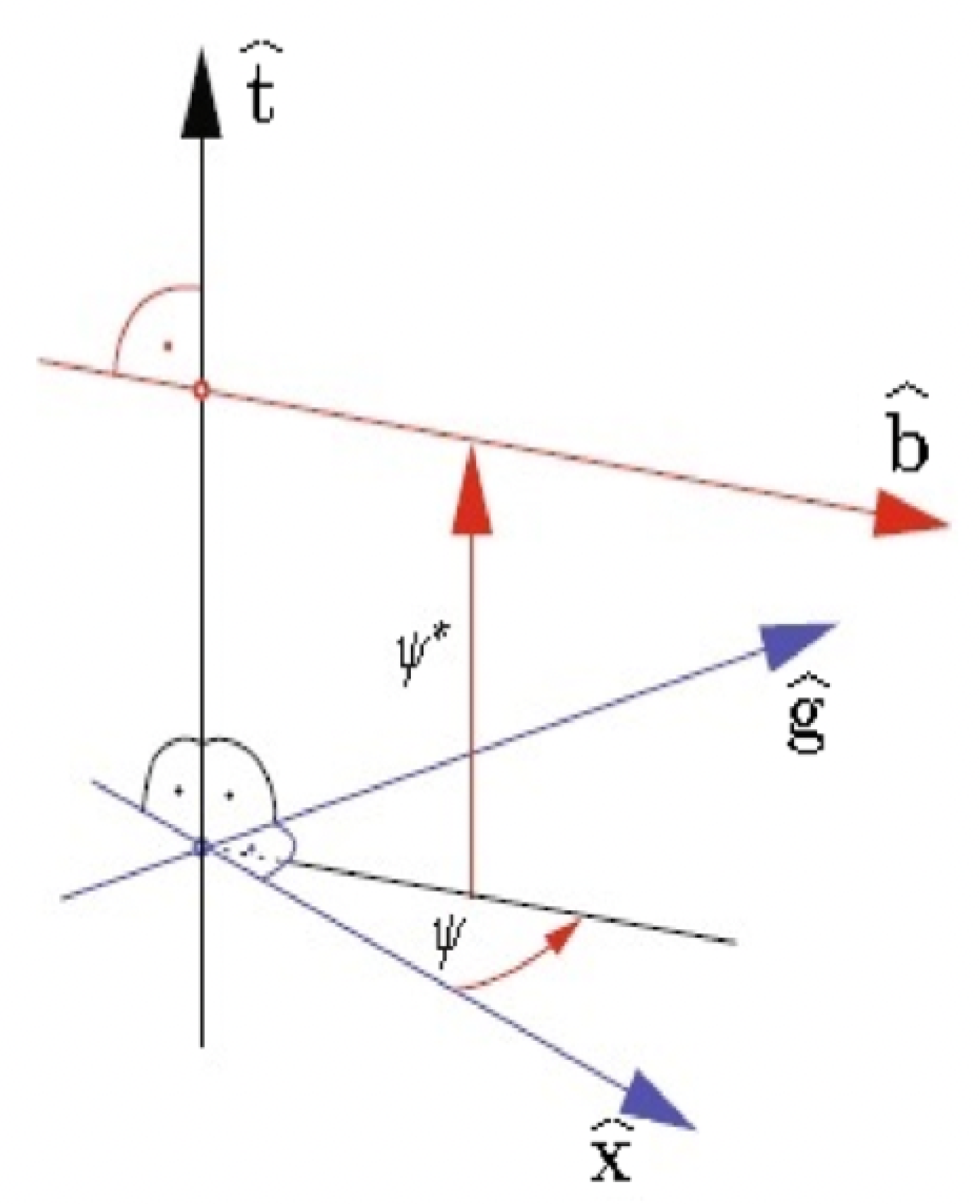
3.2. Timelike Plücker’s Conoid
We now are dealing with the kinematics-geometrical of the Hamilton and Mannhiem formulae. To this aim, the surface
is a Minkowski version of the well known Plücker conoid or cylindroid as follows: let
use the
y-axis of a stationary hyperbolic frame
and let the location of
be designated by angle
and distance
on the positive orientation of the
y-axis. The dual unit vectors
timelike) and
spacelike) can be taken with the
x- and
z-axes, respectively. Then, {
,
} identifies the coordinate system of the timelike Plücker conoid (
Figure 2). Here
represents a directed mutual perpendicular of the given lines
and
as well as the sign of
and
is related to the orientation of
. In view of Equations (9) and (11), we have
from which we have
By an easy calculation, we gain
which is the algebraic equation for
. It is clear that Equation (
15) is based only on the two integral invariants of the first order;
,
(
Figure 3). Further, one can obtain a second-order algebraic equation in
as
For the limits of
we put
. Thus, the two boundaries of
are:
Equation (
17) gives two isotropic torsal timelike planes, each of which contains one isotropic torsal timelike line
L. Hence, the geometric aspects of
are as follows:
- (i)
If , then we have two rulings through the point ; and for the two limit isotropic torsal timelike planes , the rulings and the principal axes are identical.
- (ii)
If
then we have two torsal isotropic timelike lines
,
specified as
Equation (
18) shows that the two-isotropic torsal timelike lines
and
are orthogonal to each other. So, if
and
are equal, then the timelike Plücker conoid degenerates to a family of timelike lines in the origin “
” in the timelike torsal plane
. In this case,
and
are the principal axes of an elliptic timelike line congruence. However, if
and
have opposite signs, then
and
are coincident with the principal axes of a timelike hyperbolic line congruence.
However, to transform from polar coordinates to Cartesian, we use the transformation
into Hamilton’s formula; we obtain the equation
of a hyperbolic conic section. This conic section is a Minkowski form of Dupin’s indicatrix of the surface theory in Euclidean 3-space
.
Serret–Frenet Frame
In Equation (
3), if
, then
is a timelike tangential developable ruled surface. In this case, Dupin’s indicatrix is a set of parallel isotropic timelike lines located via
. Let
u be an arc length parameter of
and
,
,
,
be the usual movable Serret–Frenet frame. Then,
where
Therefore, the curvature function
is the radius of curvature of the timelike striction curve
. Then,
(b) If
, then the striction curve is tangent to
; it is normal to the ruling through
, where
,
,
. In this case, (
) a timelike binormal ruled surface. Moreover, the Dupin’s indicatrix is a set of parallel spacelike lines located via
. Similarly, we have
where
Then, the curvature function
is the radius of torsion of the spacelike striction curve
. Similarly, we have:
3.3. Timelike Ruled Surface with Stationary Disteli-Axis
In the following, when we say () is a timelike ruled surface with stationary timelike Disteli-axis, we mean that all the rulings of () have a stationary dual angle from its Disteli-axis.
Let
define the dual arc length of
. Then, we have
By employing
instead of
t, from Equations (2) and (19), we have:
where
,
is the dual spherical curvature of
. Then,
where
is the dual curvature and
is the dual torsion of the dual curve
.
Height Dual Functions
In analogy with [
17,
18], a dual point
of
will be said to be a
evolute of the dual curve
on
; for all
i such that
,
, but
. Here
signalizes the i-th derivatives of
with respect to the dual arc length of
on
. For the first evolute
of
, we have
and
. So,
is at least a
evolute of
.
We now address a regular dual function , by . We call a height dual function on . We use for any stationary point .
Proposition 2. Let be a dual curve in with . Then, the following holds:
1-h will be stationary in the first approximation iff ,; that is,for some dual numbers and . 2-h will be stationary in the second approximation iff is evolute of ; that is, 3-h will be stationary in the third approximation iff is evolute of ; that is, 4-h will be stationary in the fourth approximation iff is evolute of ; that is, Proof. For the first derivative of
h, we obtain:
So, we obtain:
for some dual numbers
and
, the result is clear.
2-Derivation of Equation (
22) leads to:
3-Derivation of Equation (
23) leads to:
4-By similar arguments, we can also obtain:
The proof is completed. □
According to the above proposition, we obtain the following:
- (a)
The osculating circle
of
in
is specified by the equations
which are gained from the condition that the osculating circle must be at least 3rd order at
iff
.
- (b)
The osculating circle and the curve in are at least 4th order at iff and .
In this way, by taking into consideration the evolutes of in , we can gain a sequence of evolutes , , …,. The ownerships and the connection through these evolutes and their involutes are very interesting problems. For example, it is simple to see that when and , exist, is dual constant relative to . In this case, the timelike Disteli-axis is stationary up to second order and the line moves over it with stationary pitch. Thus, the timelike ruled surface () with stationary timelike Disteli-axis is created by timelike line located at a Lorentzian stationary distance and Lorentzian stationary angle with respect to the timelike Disteli-axis .
Theorem 1. A non-developable timelike ruled surface is a stationary timelike Disteli-axis if and only if = constant, and = constant.
We will now construct a timelike ruled surface with stationary timelike Disteli-axis. From Equation (20), we have ODE . The general solution of this equation is:where . Therefore, we have: From Equations (11) and (26), we have: This indicates that the timelike Disteli-axis is coincident with . From the real and the dual parts of in Equation (25), we obtain Let y be a point on . Since y, we have that the system of linear equations in (i = 1, 2, 3 and are the coordinates ofy): The matrix of coefficients of unknowns is the skew symmetric matrixand thus its rank is 2 with (k is an integer). The rank of the augmented matrixis also 2. Then, this system has infinite solutions given by Since can be arbitrary, we may take . In this case, Equation (30) becomes If we set and φ as the movement parameter, then is timelike ruled in -space. We now simply find the base curve as It can be shown that ; () so the base curve of () is its striction curve. The curvature and torsion of can be given bywhich means that is a spacelike () or timelike () circular helix. From Equations (26) and (32), it can be found that Hence, the major geometrical characteristics of can be described as follows: is a stationary timelike Disteli-axis ruled surface, is constant, is constant and is a spacelike () or timelike () circular helix.
Theorem 2. Let be any non-developable ruled surface in Minkowski 3-space . Then, is a timelike ruled Weingarten surface if and only if is a stationary timelike Disteli-axis ruled.
On the the other hand, let be a point on the timelike oriented line . Then, from Equations (28) and (32), we gain The constants h, ψ and can control the shape of the surface . The timelike ruled surface can be classified into four types according to their striction curves:
- (1)
Timelike helicoidal surface with its striction curve is a spacelike cylindrical helix: for , , , and (Figure 4). - (2)
Lorentzian sphere with its striction curve is a spacelike circle: for , , and (Figure 5). - (3)
Timelike Archimedes with its striction curve is a timelike line: for , , , and (Figure 6). - (4)
Timelike circular cone with its striction curve is a fixed point: for , , and (Figure 7).
4. Conclusions
In this work, we utilized E. Study’s map as a direct procedure for inspecting the kinematic geometry of a timelike ruled surface with stationary timelike Disteli-axis by the similarity with hyperbolic dual spherical kinematics. This provides the ability to have a set of curvature functions that locate the local shape of timelike ruled surface. Hence, the hyperbolic version of the well known equation of the Plücker conoid has been presented and its properties are explained in details. In addition, a characterization for a timelike line to be a stationary timelike Disteli-axis is inspected and outlined. Our results in this paper can contribute to the field of spatial kinematics and have practical applications in mechanical mathematics and engineering. In future work, we plan to proceed to study some applications of kinematic geometry of one parameter hyperbolic spatial movement combine with skew timelike axes such that at any instant the contact points are located on a timelike line and so forth, offered in [
19,
20,
21,
22]. Moreover, we believe this work can be used to study some applications of kinematic geometry of one parameter hyperbolic spatial movement combine with singularity theory and submanifold theory; visualizing data can help especially in the field of relativity, mathematical physics, etc. More new results and properties can be found at [
23,
24,
25].
Author Contributions
Conceptualization R.A.A.-B.; formal analysis F.M.; investigation, R.A.A.-B. and F.M.; methodology, R.A.A.-B.; project administration and funding F.M.; validation, R.A.A.-B. and F.M.; writing original draft R.A.A.-B. and F.M. All authors have read and agreed to the published version of the manuscript.
Funding
The author, F.M., expresses her gratitude to Princess Nourah bint Abdulrahman University Researchers Supporting Project number (PNURSP2023R27), Princess Nourah bint Abdulrahman University, Riyadh, Saudi Arabia.
Data Availability Statement
No data were used to support this study.
Acknowledgments
Princess Nourah bint Abdulrahman University Researchers Supporting Project number (PNURSP2023R27), Princess Nourah bint Abdulrahman University, Riyadh, Saudi Arabia.
Conflicts of Interest
The authors declare no conflict of interest.
References
- Bottema, O.; Roth, B. Theoretical Kinematics; North-Holland Press: New York, NY, USA, 1979. [Google Scholar]
- Karger, A.; Novak, J. Space Kinematics and Lie Groups; Gordon and Breach Science Publishers: New York, NY, USA, 1985. [Google Scholar]
- Pottman, H.; Wallner, J. Computational Line Geometry; Springer: Berlin/Heidelberg, Germany, 2001. [Google Scholar]
- Abdel-Baky, R.A.; Al-Solamy, F.R. A new geometrical approach to one-parameter spatial motion. J. Eng. Maths 2008, 60, 149–172. [Google Scholar] [CrossRef]
- Abdel-Baky, R.A.; Al-Ghefari, R.A. On the one-parameter dual spherical motions. Comp. Aided Geom. Des. 2011, 28, 23–37. [Google Scholar] [CrossRef]
- Al-Ghefari, R.A.; Abdel-Baky, R.A. Kinematic geometry of a line trajectory in spatial motion. J. Mech. Sci. Technol. 2015, 29, 3597–3608. [Google Scholar] [CrossRef]
- Abdel-Baky, R.A. On the curvature theory of a line trajectory in spatial kinematics. Commun. Korean Math. Soc. 2019, 34, 333–349. [Google Scholar]
- Abdel-Baky, R.A.; Naghi, M.F. A study on a line congruence as surface in the space of lines. AIMS Math. 2021, 6, 11109–11123. [Google Scholar] [CrossRef]
- Ferhat, T.; Abdel-Baky, R.A. On a spacelike line congruence which has the parameter ruled surfaces as principal ruled surfaces. Int. Electron. J. Geom. 2019, 12, 135–143. [Google Scholar]
- Abdel-Baky, R.A. Timelike line congruence in the dual Lorentzian 3-space . J. Geom. Methods Mod. Phys. 2019, 16, 2. [Google Scholar]
- Alluhaibi, N.; Abdel-Baky, R.A. On the one-parameter Lorentzian spatial motions. Int. J. Geom. Methods Mod. 2019, 16, 2. [Google Scholar] [CrossRef]
- Abdel-Baky, R.A.; Unluturk, Y. A new construction of timelike ruled surfaces with stationarfy Disteli-axis. Honam Math. J. 2020, 42, 551–568. [Google Scholar]
- Alluhaibi, N.S.; Abdel-Baky, R.A.; Naghi, M.F. On the Bertrand offsets of timelike ruled surfaces in Minkowski 3-space. Symmetry 2022, 14, 673. [Google Scholar] [CrossRef]
- Abdel-Baky, R.A.; Mofarreh, F. A study on the Bertrand offsets of timelike ruled surfaces in Minkowski 3-space. Symmetry 2022, 14, 783. [Google Scholar] [CrossRef]
- O’Neil, B. Semi-Riemannian Geometry Geometry, with Applications to Relativity; Academic Press: New York, NY, USA, 1983. [Google Scholar]
- Walfare, J. Curves and Surfaces in Minkowski Space. Ph.D. Thesis, K.U. Leuven, Faculty of Science, Leuven, Belgium, 1995. [Google Scholar]
- Bruce, J.W.; Giblin, P.J. Curves and Singularities, 2nd ed.; Cambridge University Press: Cambridge, UK, 1992. [Google Scholar]
- Cipolla, R.; Giblin, P.J. Visual Motion of Curves and Surfaces; Cambridge University Press: Cambridge, UK, 2000. [Google Scholar]
- McCarthy, J.M.; Roth, B. The Curvature Theory of Line Trajectories in Spatial Kinematics. J. Mech. Des. 1981, 103, 718–724. [Google Scholar] [CrossRef]
- Stachel, H. On Spatial Involute Gearing. In Proceedings of the 6th International Conference on Applied Informatics, Eger, Hungary, 27–31 January 2004. [Google Scholar]
- Figlioini, G.; Stachel, H.; Angeles, J. The Computational Fundamentals of Spatial Cycloidal Gearing. In Computational Kinematics: Proceedings of the 5th Internat Workshop on Computational Kinematic; Springer: Berlin/Heidelberg, Germany, 2009; pp. 375–384. [Google Scholar]
- Alluhaibi, N.A.; Abdel-Baky, R.A. On the kinematic geometry of one-parameter Lorentzian spatial movement. Inter. J. Adv. Manuf. Tech. 2022, 121, 7721–7731. [Google Scholar] [CrossRef]
- Li, Y.; Tuncer, O. On (contra) pedals and (anti)orthotomics of frontals in de Sitter 2-space. Math. Meth. Appl. Sci. 2023, 1, 1–15. [Google Scholar] [CrossRef]
- Li, Y.; Aldossary, M.T.; Abdel-Baky, R.A. Spacelike Circular Surfaces in Minkowski 3-Space. Symmetry 2023, 15, 173. [Google Scholar] [CrossRef]
- Li, Y.; Chen, Z.; Nazra, S.H.; Abdel-Baky, R.A. Singularities for Timelike Developable Surfaces in Minkowski 3-Space. Symmetry 2023, 15, 277. [Google Scholar] [CrossRef]
| Disclaimer/Publisher’s Note: The statements, opinions and data contained in all publications are solely those of the individual author(s) and contributor(s) and not of MDPI and/or the editor(s). MDPI and/or the editor(s) disclaim responsibility for any injury to people or property resulting from any ideas, methods, instructions or products referred to in the content. |
© 2023 by the authors. Licensee MDPI, Basel, Switzerland. This article is an open access article distributed under the terms and conditions of the Creative Commons Attribution (CC BY) license (https://creativecommons.org/licenses/by/4.0/).


