A Fractional-Order Density-Dependent Mathematical Model to Find the Better Strain of Wolbachia

Abstract

The primary objective of the current study was to create a mathematical model utilizing fractional-order calculus for the purpose of analyzing the symmetrical characteristics of $\mathit{Wolbachia}$ dissemination among $\mathit{Aedesaegypti}$ mosquitoes. We investigated various strains of $\mathit{Wolbachia}$ to determine the most sustainable one through predicting their dynamics. $\mathit{Wolbachia}$ is an effective tool for controlling mosquito-borne diseases, and several strains have been tested in laboratories and released into outbreak locations. This study aimed to determine the symmetrical features of the most efficient strain from a mathematical perspective. This was accomplished by integrating a density-dependent death rate and the rate of cytoplasmic incompatibility (CI) into the model to examine the spread of $\mathit{Wolbachia}$ and non-$\mathit{Wolbachia}$ mosquitoes. The fractional-order mathematical model developed here is physically meaningful and was assessed for equilibrium points in the presence and absence of disease. Eight equilibrium points were determined, and their local and global stability were determined using the Routh–Hurwitz criterion and linear matrix inequality theory. The basic reproduction number was calculated using the next-generation matrix method. The research also involved conducting numerical simulations to evaluate the behavior of the basic reproduction number for different equilibrium points and identify the optimal CI value for reducing disease spread.

1. Introduction

In the realm of biology, it is quite common to observe the prevalence of symmetrical characteristics in various organisms. Mathematical biology is a vast area of research that will provide insight into most relevant real-world biological problems. The most important symmetrical property, i.e., the structure of disease spread among a particular species or among more than one species can be studied through mathematical models. Our study mainly concentrated on finding a biological control to suppress mosquito-borne diseases via mathematical tools. The mosquito leads the world’s deadliest animals list by causing more than 0.7 million deaths per annum. Recent data show that annually, 390 million cases of mosquito-borne diseases are recorded. It is estimated that 0.5 million people face severe dengue illness; among them, nearly 3% of people die [1,2]. Mosquito-borne diseases include DENV, yellow fever virus, Zika virus, West Nile virus, Japanese encephalitis, Chikungunya, etc. Dengue is the most common and life-threatening disease among mosquito-borne diseases [3,4]. The primary vector is Aedes aegypti, and the secondary vector is Aedes albopictus [5]. If a virus-carrying mosquito bites an uninfected human, that human will become infectious after the latent period (2–4 days). If an uninfected mosquito bites an infected human, then the mosquito will become infectious [6,7].

There is no effective vaccination strategy against dengue due to its four variants (DENV-1, DENV-2, DENV-3, DENV-4). The reason is the invented vaccinations are able to control only one of the variants each. This leads to the fact that there may be a chance of getting a severe infection from other virus variants. The preventive measures are using bed nets, insecticides, repellents, medical intervention, etc. Regardless, these methods are not sustainable, and nowadays mosquitoes are not reacting to insecticides [8,9]. In [10], the authors studied the effectiveness of implementing vaccination against various mosquito-borne diseases. We can thus find a novel and long-lasting strategy to manage illnesses spread by mosquitoes.

Currently, the research focuses on the intervention strategies, such as genetic modifications, the release of sterile mosquitoes, and the release of $\mathit{Wolbachia}$-infected mosquitoes [11]. Currently, the most promising way to control mosquito-borne diseases is releasing the endosymbiotic bacterium called $\mathit{Wolbachia}$ into the dengue outbreak areas [12,13]. $\mathit{Wolbachia}$ controls the spread of the virus among mosquitoes and the human population in two ways: population suppression and virus blocking. When a $\mathit{Wolbachia}$-infected mosquito bites a virus-infected human, it may become infectious, but there is no possibility for virus transmission from that mosquito to an uninfected human. This bacterium stops the virus’s replication and blocks the virus inside the salivary gland. The article [14] studies the important properties of the pathogen blocking of $\mathit{Wolbachia}$ in the Aedes aegypti population. This property of $\mathit{Wolbachia}$ is called virus blocking. The $\mathit{Wolbachia}$ bacterium induces cytoplasmic incompatibility in mosquito populations [14]. That is,

• When a $\mathit{Wolbachia}$-infected male mosquito mates with the wild female, the produced eggs will not hatch (CI).
• When a $\mathit{Wolbachia}$-infected female mates with a wild male, then the produced offspring will have $\mathit{Wolbachia}$ infection (CI rescue).

Due to the effective properties of $\mathit{Wolbachia}$, this bacterium could provide mosquito-borne disease control methods [15]. More mathematical models are being developed to study the release strategies, such as male release [16], female release [17,18], the constant release strategy, the adaptive release strategy, and the crude adaptive release strategy [19].

Mathematical modeling is an effective tool for understanding and analyzing and may be used to find an optimal way to control the situation [20,21,22,23]. The research listed below shows how fractional mathematical models can be used to investigate and manage mosquito-borne diseases through $\mathit{Wolbachia}$ intervention. These models could shed light on how to create efficient prevention plans for diseases, including dengue fever, the Zika virus, and chikungunya. In [18], for the propagation of $\mathit{Wolbachia}$ in mosquito populations, the authors suggested a fractional-order differential equation model. They demonstrated that the model accurately predicts the phenomena of $\mathit{Wolbachia}$-induced cytoplasmic incompatibility, and they used numerical simulations to illustrate how efficient $\mathit{Wolbachia}$ is as a preventative measure. In [24], the authors explore the use of fractional calculus models in understanding the complex dynamics of biological tissues. The authors proposed a model that incorporates both fractional-order derivatives and spatial diffusion and investigated its behavior using numerical simulations. In [25], the authors presented a study on a variable-order fractional version of the Benjamin–Bona–Mahony–Burger equation. The authors employed a pseudo-spectral method to numerically investigate the equation and obtain accurate solutions. The study is important for understanding the behavior of variable-order fractional differential equations, which have applications in various areas of science and engineering. In [26,27], the authors proposed a hybrid collocation method for solving multi-term, time-fractional partial differential equations and presented numerical solutions of variable-order, time-fractional (1+1)- and (1+2)-dimensional advection-dispersion and diffusion models. Throughout history, researchers have done research to eradicate mosquito-borne diseases in various aspects. For example, in [28,29,30,31,32,33,34,35], the interaction between wild mosquitoes and sterile mosquitoes (genetically modified male mosquitoes, when a wild female mosquito mates with a sterile male mosquito, the eggs produced will not hatch) is modeled in several situations, such as two-stage life cycles, incomplete sterility and a density-dependent model. The authors of [36], analyzed the interaction model at various release strategies. In [37], the authors of developed a three-compartmental model by dividing wild mosquito populations into aquatic and adult stages as two compartments and released genetically modified mosquitoes (sterile male mosquitoes) as a third compartment. The method used in the sterile insect release technique was utilized to model the interaction between $\mathit{Wolbachia}$-infected mosquitoes and wild mosquitoes, including the human population in [38,39,40,41,42]. The effects of using vaccination incorporated with a $\mathit{Wolbachia}$ releasing strategy was studied in [43,44]. How the stochastic environment affects the $\mathit{Wolbachia}$ transmission dynamics, and an impulsive release strategy using integer and fractional-order models, were studied in [18,45], respectively. Researchers modeled the transmission dynamics as different compartmental models considering only adults (females and males) in the aquatic stage; females and males (common groups containing both $\mathit{Wolbachia}$ and wild); wild aquatic and $\mathit{Wolbachia}$ aquatic wild females and males; $\mathit{Wolbachia}$-infected females and males; etc., with the continuous time model [46] and the discrete time model [47]. Larvae as one compartment and adult as another compartment were considered, and impulsive release of sterile mosquitoes was studied in [48].

In nature, there exist more $\mathit{Wolbachia}$ strains, such as wMel—partial CI or none (native host: Drosophila melanogaster); wMelPop—partial CI or none (Drosophila melanogaster); wAu—no CI, (Drosophila simulans); wMelCS—low or none (Drosophila melanogaster); wInn—male killing, no CI (Drosophila innubila); wPip—high CI (Culex pipiens); and wAlbB—high CI (Aedes albopictus) [49].

Motivated by the existing literature, our main aim was to find the answer to, ’What is the best strain of $\mathit{Wolbachia}$ to control mosquito-borne diseases?’ Secondly, we studied whether when we release laboratory-reared mosquitoes into the wild mosquito population, there will exist some decay in both mosquitoes population due to the competition developed by density.

Main contributions of this article are listed as follows:

• The failure of integer order systems to accurately predict certain phenomena is a widely recognized issue, and thus, the use of fractional-order systems is a natural extension in many fields. This article presents a novel 10-compartmental, fractional-order, density dependent mathematical model. Then, we checked the model’s eligibility by performing various mathematical analyses.
• A new parameter describing the CI mechanism in both the mosquito population and controlling the disease spread by reducing the population size of wild mosquitoes is introduced. Owing to this parameter’s inclusion, we are able to find the better strain in the sense of having perfect CI.
• In the existing literature, vaccination strategies are included while developing a model. However, we neglected the vaccination strategy because there exists a licensed vaccination called Dengvaxia (CYD-TDV), and five more are in trials. Regardless, WHO recommends these vaccines to people who have a history of dengue infection. Although there are four different stereotypes of dengue virus (DENV-1, DENV-2, DENV-3, DENV-4), the invented vaccinations are not able to control all four DENVs. They provide immunity against one and do not provide immunity against the other three. For this reason, there is a chance of having severe dengue infection by the remaining three variants. This aspect of vaccination is considered seriously and neglected in the vaccination strategy from the disease-controlling process.
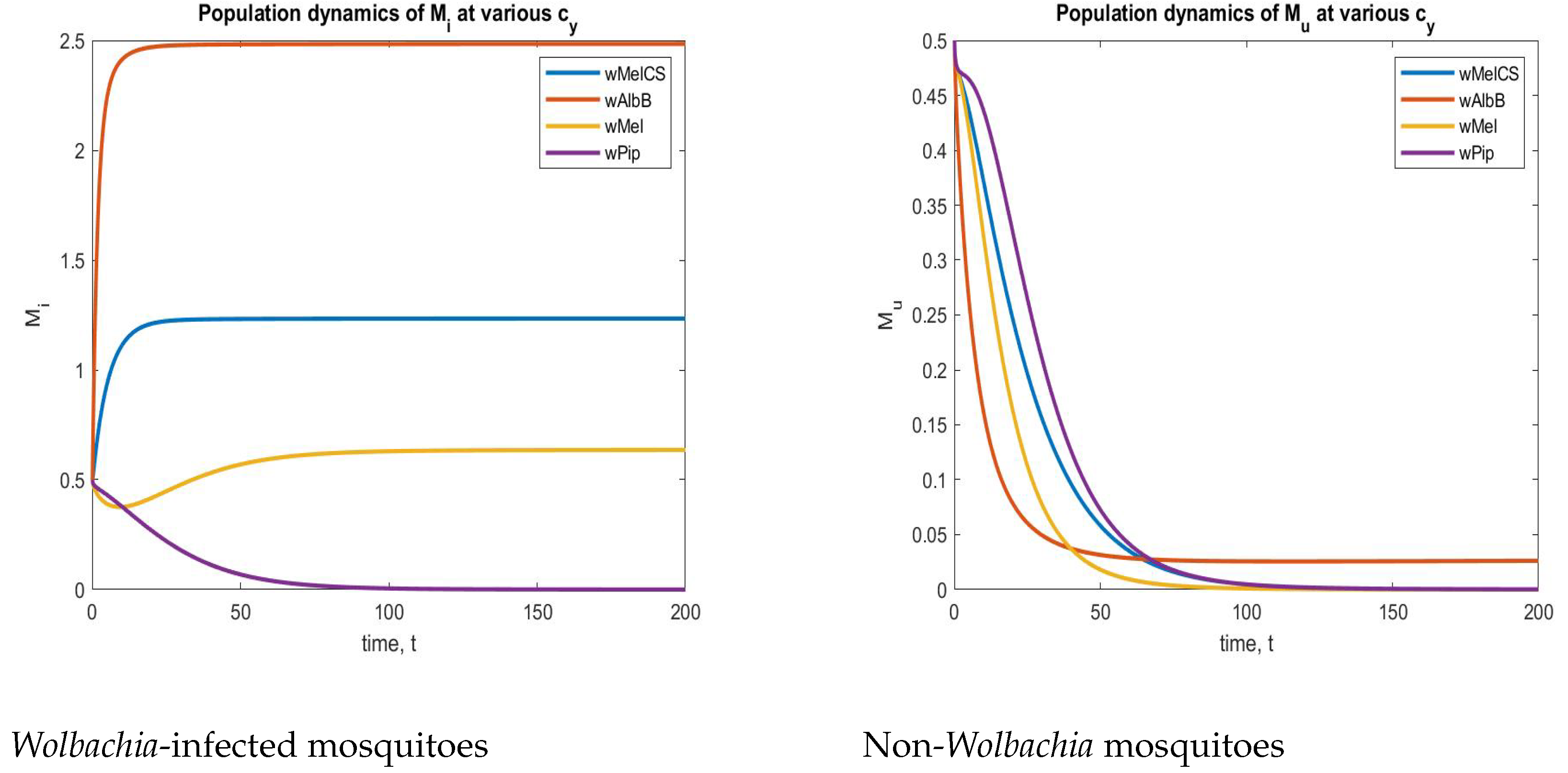
• Our proposed model shows that when there is the existence of $\mathit{Wolbachia}$-infected mosquitoes, there is a notable change in the spread of disease. We derived the basic reproduction number of the disease and analyzed it at possible equilibrium points. The derived numerical results show that our releasing strategy is physically meaningful, and at some point, it works as a better strategy to control mosquito-borne diseases.
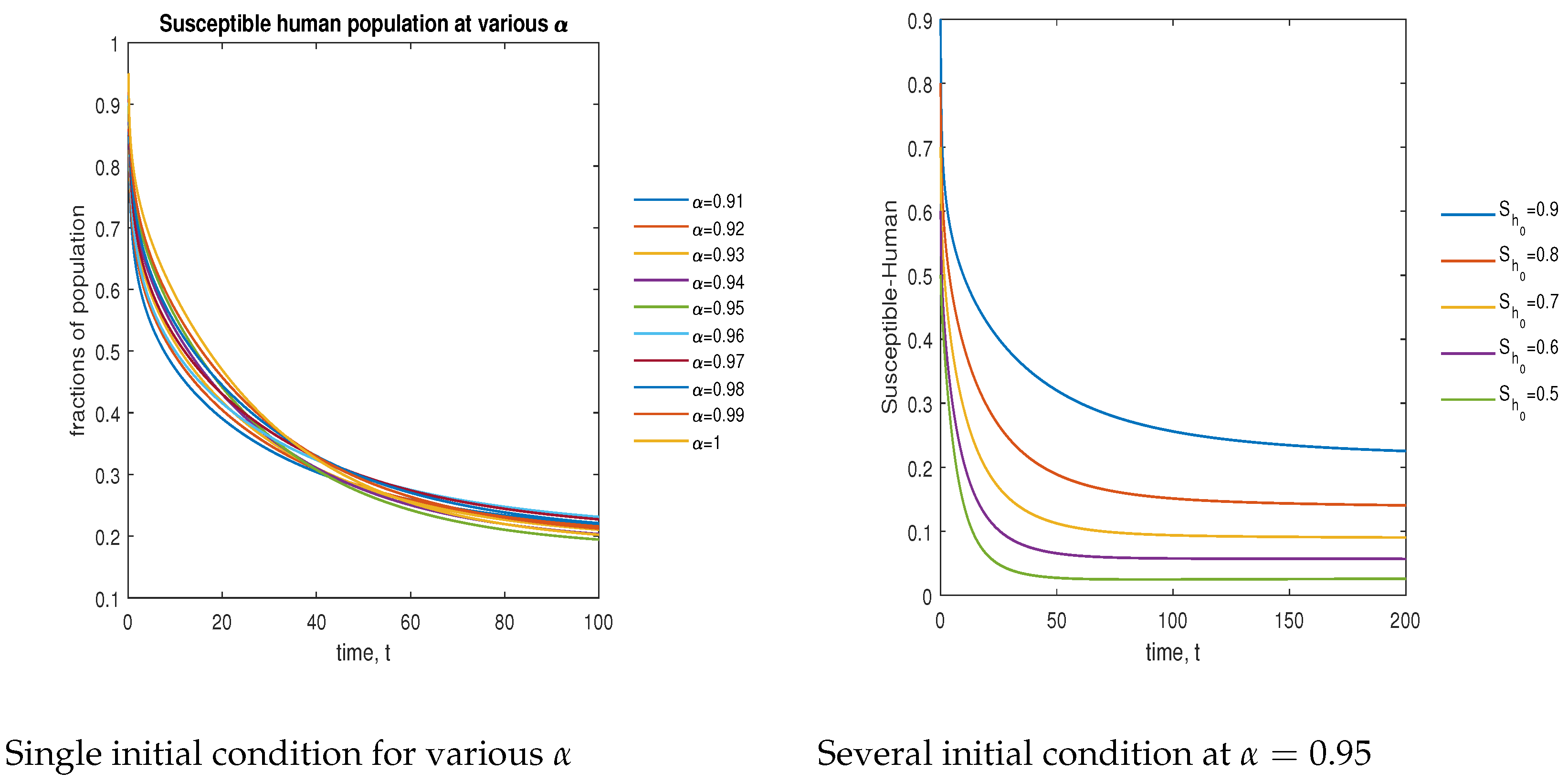
• Dynamical analysis of the proposed model is depicted as a time-series plot by numerically solving our model.

This article is structured as follows: The detailed methodology is presented in Section 2. Preliminaries take place in Section 3, and complete information about the development of integer and fractional-order models is presented in Section 4. Section 5 is about some properties of the proposed fractional-order model. Analysis of the model in terms of basic reproduction number, disease free equilibria, endemic equilibria, and their local and global stabilities is presented in Section 6. In Section 7, the sensitivity of the parameters is discussed. Numerical simulations are presented in Section 8, and the results are concluded in Section 9.

2. Methodology

(i)

First we propose a fractional-order mathematical model using Caputo fractional derivative to expose the interaction dynamics of $\mathit{Wolbachia}$-infected, $\mathit{Wolbachia}$-uninfected mosquitoes and humans. Moreover, the influences of imperfect maternal transmission and density-dependent death rates are considered in mosquito populations.

(ii)

To find the basic reproduction number, we used a next-generation method [50].

(iii)

The local stability of four cases of the disease-free equilibrium and three cases of endemic equilibrium are analyzed by finding determinants and traces of the corresponding Jacobian matrix (Routh–Hurwitz criterion).

(iv)

The global stability of the developed model is derived from linear matrix inequality theory and Lyapunov theory.

(v)

Numerical simulations to prove the effectiveness of the parameters used in the model formulations and to show how the system dynamics are influenced by various $\mathit{Wolbachia}$ strains.

3. Preliminaries

Definition 1.

(Caputo derivative) [51] M. Caputo in [52] derived a certain solution for a fractional-order differential equation as

$$\begin{array}{ccc}\hfill {}_b^c{D}_t^{\alpha }g\left(t\right)& =& \frac{1}{\Gamma (\alpha -m)}{\int }_b^t\frac{g^{\left(n\right)}\left(s\right)ds}{{(t-s)}^{\alpha +1-m}},m-1<\alpha <m.\hfill \end{array}$$

For $\alpha \to m$, the Caputo derivative becomes a conventional $m^{th}$ derivative of $g\left(t\right)$. Here, the operator ${}_b^c{D}_t^{\alpha }g\left(t\right)$ represents a fractional operator with an initial condition b, independent variable t, fractional-order α and c denoting that it is Caputo-sense.

Lemma 1

([51]). The following equation denotes the fractional differential equation in a Caputo sense:

$$\begin{array}{ccc}\hfill {}_a^c{D}_t^{\alpha }x\left(t\right)& =& f(t,x(t\left)\right)\hfill \\ \hfill x\left(t_0\right)& =& x_0\hfill \end{array}$$

The above equation is said to have an equilibrium point or fixed point $x^{*}$ if it satisfies $f(t,x^{*})=0$.

Lemma 2

([53]). $A_1$, $A_2$ and $A_3$ are $n\times n$ matrices with $A_1=A_1^{\top }>0$ and $A_2=A_2^{\top }>0$. Then,

$$\begin{array}{ccc}\hfill A_1+A_3^{\top }{A}_2^{-1}{A}_3& <& 0\hfill \end{array}$$

if and only if

$$\begin{array}{c}\hfill \left[\begin{array}{cc}{A}_1& A_3^{\top }\\ A_3& -A_2\end{array}\right]<0\end{array}$$

or

$$\begin{array}{c}\hfill \left[\begin{array}{cc}-A_2& A_3\\ A_3^{\top }& A_1\end{array}\right]<0.\end{array}$$

Lemma 3

([54]).

$$\begin{array}{ccc}\hfill {\Phi }^{\top }\left(t\right)\Theta F(\Phi \left(t\right))& \le & \frac{1}{2\sigma }{\Phi }^{\top }\left(t\right)(\Theta {\Theta }^{\top })\Phi \left(t\right)+\frac{\sigma }{2}{F}^{\top }(\Phi \left(t\right))F(\Phi \left(t\right))\hfill \end{array}$$

where $\sigma >0$ be scalar, $\Phi ,F(\Phi \left(t\right))\in {\mathbb{R}}^n$ and $\Theta$ is a matrix.

Definition 2.

(Laplace transformation) The Laplace transformation of the function which is defined in the sense of a Caputo derivative is as follows:

$$\begin{array}{ccc}\hfill \mathfrak{L}\{{}_a^c{D}_t^{\alpha }G\left(t\right),r\}& =& r^{\alpha }G\left(r\right)-\sum _{j=0}^{n-1}{r}^{\alpha -j-1}{G}^{\left(j\right)}\left(0\right),\hfill \end{array}$$

where $\alpha \in (n-1,n)$ and n is a natural number.

The Mittag–Leffler function is shown by

$$\begin{array}{ccc}\hfill E_{a,b}& =& \sum _{j=0}^{\infty }\frac{g^j}{\Gamma (aj+b)}\hfill \end{array}$$

and the Laplace transform is

$$\begin{array}{ccc}\hfill \mathfrak{L}\left[t^b{E}_{a,b}\left(\pm a{t}^a\right)\right]& =& \frac{u^{a-b}}{u^a\mp a}\hfill \end{array}$$

4. Model Formulation

The present section is devoted to developing a mathematical model as close as possible to a real-life situation to analyze the symmetrical features. To ensure this, the density-dependent death rate with a fitness cost and the effectiveness of CI are incorporated. Through the developed model, we tried to find the answers to the following questions:

• How does the release of $\mathit{Wolbachia}$-mosquitoes affect the wild mosquito population in the sense of reducing the lifespan, occupying the habitats, male feminization, and CI?
• What is the best $\mathit{Wolbachia}$ strain to be used in the real world?
• How CI will influence the disease-spread dynamics?

Before developing a physically meaningful mathematical model, a few hypotheses are necessary.

(H1)

The three populations in the model are:

M_i 

$\mathit{Wolbachia}$-infected mosquitoes (both laboratory-reared and offspring having $\mathit{Wolbachia}$ after CI rescue).

M_u 

Non-$\mathit{Wolbachia}$ mosquitoes (both local and offspring produced by weak CI).

H 

Human population.

In contrast to mosquitoes, which are believed to have a variable population size, humans have a steady population size. as, in contrast to a single human generation, mosquitoes have many generations over that period.

(H2)

People of all ages and all genders make up the human population.

(H3)

The host population is monolithically intermingled. This implies that all individuals, irrespective of age, genetic development, sociocultural context, or geographic region, have almost the same pathogenic traits.

(H4)

Only mature females were taken into account for modeling. As they require a blood meal to warm and develop the eggs before they can lay eggs, only sexually active female mosquitoes will engage with people.

(H5)

Mosquitoes are divided into six groups representing the state variables: aquatic stage (eggs, larvae, pupae) of $\mathit{Wolbachia}$ as $M_i$ and non-$\mathit{Wolbachia}$ as $M_u$. Adult female mosquitoes are divided into four groups: $\mathit{Wolbachia}$-infected and susceptible to virus—$M_{i,s}$; $\mathit{Wolbachia}$-infectious (virus)—$M_{i,i}$; non-$\mathit{Wolbachia}$-infected and susceptible to virus—$M_{u,s}$; and non-$\mathit{Wolbachia}$-infected (virus)—$M_{u,i}$. The human population is divided into four compartments as susceptible $S_h$, infectious $I_h$, hospitalized $H_h$, and recovered $R_h$. In both populations, we neglected the latent period (exposed) because the time span of latency is much smaller compared with the total life span of the human population and the mosquito population. Additionally, we assumed that $S_h+I_h+H_h+R_h=T_h\left(Constant\right)$ and $M_{i,s}+M_{i,i}+M_{u,s}+M_{u,i}=T_{m_i}+T_{m_u}=T_m$ (function of time).

(H6)

All newborns are susceptible to the virus; there is no vertical transmission of the disease or heredity in the human population or mosquitoes.

(H7)

However, in the case of $\mathit{Wolbachia}$ spread. there is vertical transmission and heredity in mosquitoes. Notably, there is no horizontal transmission of $\mathit{Wolbachia}$ between mosquito and human population.

(H8)

A mosquito acquires an infection when it bites an infected individual, and a person who has been bitten by an infected mosquito contracts the infection as well. Male mosquitoes do not participate in this activity, since they solely feed on nectar.

(H9)

There is a chance to generate a density-dependent concurrence for food, habitats, etc., when we intentionally introduce $\mathit{Wolbachia}$-infected mosquitoes as eggs in the form of ’Zancu KIT’ and adult mosquitoes via drones, transportation, and manual release into mosquito-borne disease epidemic areas. This fact causes both $\mathit{Wolbachia}$ and non-$\mathit{Wolbachia}$ mosquitoes to die in a density-dependent manner.

(H10)

The parameter $c_y$ denotes the cytoplasmic incompatibility (CI) induced by $\mathit{Wolbachia}$. This CI will serve as a main component in reducing the population size of mosquitoes. As CI is the process that makes the males feminized and reduce the possibility of producing viable progeny. There exist many $\mathit{Wolbachia}$ strains, such as $wPop$, $wMel$, $wAlbA$, $wAlbB$, $wAu$ and $wAuWpip$. Among these strains, the superinfected strain $wAlbB$ has the highest CI [55].

4.1. Integer-Order Model

Motivated by [38], we have developed a $\mathit{Wolbachia}$, non-$\mathit{Wolbachia}$ and human population interaction model to study symmetrical features:

Wolbachia mosquitoes:

$$\begin{array}{c}\hfill \left\{\begin{array}{cc}\frac{d{M}_i}{dt}\hfill & ={\Lambda }_1+r_m\eta M_i-{\lambda }_{i_a}{M}_i-{\lambda }_{d_i}\left[M_i+M_u\right]M_i-t_w{M}_i\hfill \\ \frac{d{M}_{i,s}}{dt}\hfill & =t_w{T}_{m_i}-\frac{{\alpha }_i{\rho }_{m_h}{I}_h}{T_h}{M}_{i,s}-{\lambda }_{m_i}{M}_{i,s}\hfill \\ \frac{d{M}_{i,i}}{dt}\hfill & =\frac{{\alpha }_i{\rho }_{m_h}{I}_h}{T_h}{M}_{i,s}-{\lambda }_{m_i}{T}_m{M}_{i,i}\hfill \end{array}\right.\end{array}$$

Non-Wolbachia mosquitoes:

$$\begin{array}{c}\hfill \left\{\begin{array}{cc}\frac{d{M}_u}{dt}\hfill & ={\Lambda }_2+r_m(1-\eta )M_i-{\lambda }_{u_a}{M}_u-{\lambda }_{d_u}\left[M_i+M_u\right]M_i-t_w{M}_u\hfill \\ \hfill & +r_m(1-c_y)M_u\frac{M_i}{M_i+M_u}-r_m{M}_u\frac{M_u}{M_i+M_u}\hfill \\ \frac{d{M}_{u,s}}{dt}\hfill & =t_w\left(1-\frac{T_{m_i}}{T_m}\right)T_{m_u}-\frac{{\alpha }_u{\rho }_{m_h}{I}_h}{T_h}{M}_{u,s}-{\lambda }_{m_u}{M}_{u,s}\hfill \\ \frac{d{M}_{u,i}}{dt}\hfill & =\frac{{\alpha }_u{\rho }_{m_h}{I}_h}{T_h}{M}_{u,s}-{\lambda }_{m_u}{T}_m{M}_{u,i}\hfill \end{array}\right.\end{array}$$

Human:

$$\begin{array}{c}\hfill \left\{\begin{array}{cc}\frac{d{S}_h}{dt}\hfill & =r_h-\frac{{\alpha }_i{\rho }_{m_i}{M}_{i,i}}{T_h}{S}_h-\frac{{\alpha }_u{\rho }_{m_u}{M}_{u,i}}{T_h}{S}_h-{\lambda }_h{S}_h\hfill \\ \frac{d{I}_h}{dt}\hfill & =\frac{{\alpha }_i{\rho }_{m_i}{M}_{i,i}}{T_h}{S}_h+\frac{{\alpha }_u{\rho }_{m_u}{M}_{u,i}}{T_h}{S}_h-{\eta }_h{I}_h-{\gamma }_{h_1}{I}_h-{\lambda }_h{I}_h\hfill \\ \frac{d{H}_h}{dt}\hfill & ={\eta }_h{I}_h-{\gamma }_{h_2}{H}_h-{\lambda }_h{H}_h\hfill \\ \frac{d{R}_h}{dt}\hfill & ={\gamma }_{h_1}{I}_h+{\gamma }_{h_2}{H}_h-{\lambda }_h{R}_h,\hfill \end{array}\right.\end{array}$$

(1)

where the initial conditions are $M_i\ge 0$, $M_u\ge 0$, $M_{i,s}\ge 0$, $M_{i,i}\ge 0$, $M_{u,s}\ge 0$, $M_{u,i}\ge 0$, $S_h\ge 0$, $I_h\ge 0$, $H_h\ge 0$, and $R_h\ge 0$. Additionally, the populations are represented as $T_h:[0,\infty )\to \mathbb{R}$ and $T_m:[0,\infty )\to \mathbb{R}$ and each $M_{i,s},M_{i,i},M_{u,s},M_{u,i},S_h,I_h,H_h,R_h:[0,\infty )\to \mathbb{R}$. For instance, refer Figure 1 to understand the structure of the model (1). The descriptions of variables and parameters are listed in

Table 1. Descriptions of variables.

Variables	Description
$M_i$	The number of $\mathit{Wolbachia}$-infected mosquitoes at time ‘t’
$M_{i,s}$	The number of $\mathit{Wolbachia}$-infected mosquitoes susceptible
	to Dengue virus at a time ‘t’
$M_{i,i}$	The number of $\mathit{Wolbachia}$-infected mosquitoes infected by
	Dengue virus at time ‘t’
$M_u$	The number of non-$\mathit{Wolbachia}$ mosquitoes at time ‘t’
$M_{u,s}$	The number of non-$\mathit{Wolbachia}$ mosquitoes susceptible to
	Dengue virus at time ‘t’
$M_{u,i}$	The number of non-$\mathit{Wolbachia}$ mosquitoes infected by
	Dengue virus at time ‘t’
$S_h$	The number of the susceptible human population at a time ‘t’
$I_h$	The number of the infectious human population at a time ‘t’
$H_h$	The number of hospitalized human population at a time ‘t’
$R_h$	The number of recovered human population at a time ‘t’

and

Table 2. Descriptions of parameters.

Parameters	Description	Values	Unit	Source
$t_w$	Reproduction rate of mosquitoes	$1.25$	1/day	[38]
${\Lambda }_2$	Reproduction rate of wild mosquitoes	$1.25$	1/day	[38]
${\Lambda }_1$	Reproduction rate of $\mathit{Wolbachia}$ mosquitoes	$0.95\times {\Lambda }_2$	1/day	[56]
$r_m$	Reproduction rate of mated female mosquitoes	$0.4$	1/day	[39]
$\eta$	fraction of produced offspring having $\mathit{Wolbachia}$ infection	$(0,1)$	NA	[39]
$r_m(1-\eta )$	Fraction of produced offspring not having $\mathit{Wolbachia}$ infection	$0.9\times (1-\eta )$	NA	[39]
${\lambda }_{i_a}$	Natural death rate of $\mathit{Wolbachia}$ aquatic mosquitoes	$1/14$	1/day	[39]
${\lambda }_{d_i}$	Density-dependent death rate of $\mathit{Wolbachia}$ aquatic mosquitoes		1/day
${\lambda }_{u_a}$	Natural death rate of non-$\mathit{Wolbachia}$ aquatic mosquitoes	$1/14$	1/day	[57]
${\lambda }_{d_u}$	Density dependent death rate of non-$\mathit{Wolbachia}$ aquatic mosquitoes		1/day
$t_w$	Maturation rate of aquatic stage mosquitoes from which adult mosquitoes emerge	$0.1$	1/day	[57]
${\alpha }_u$	The average bitting rate of non-$\mathit{Wolbachia}$ mosquitoes	$0.63$	1/day	[58]
${\alpha }_i$	Average bitting rate of $\mathit{Wolbachia}$ mosquitoes	$0.95\times {\alpha }_u$	1/day	[59]
${\rho }_{m_h}$	Probability virus transmission from infected human to $\mathit{Wolbachia}$ and non-$\mathit{Wolbachia}$ mosquitoes	$0.2614$	NA	[39]
${\rho }_{m_i}$	Virus transmission probability from infected $\mathit{Wolbachia}$ mosquitoes to susceptible human	$0.5\times {\rho }_{m_h}$	NA	[60]
${\rho }_{m_u}$	Virus transmission probability from infected non-$\mathit{Wolbachia}$ mosquitoes to susceptible human	$0.2614$	NA	[39]
${\lambda }_{m_u}$	Mortality rate of non-$\mathit{Wolbachia}$ adult mosquitoes	$1/14$	1/day	[57]
${\lambda }_{m_i}$	Mortality rate of $\mathit{Wolbachia}$ adult mosquitoes	$1.1\times {\lambda }_{m_u}$	1/day	[56,61]
$r_h$	Birth rate of human	$0.000012$	1/day	[62]
${\lambda }_h$	Natural death rate of human population	$0.000012$	1/day	[62]
${\eta }_h$	Hospitalization rate of identified infected human	$0.0904$	1/day	[63]
${\gamma }_{h_1}$	The rate of natural recovery of infected human due to immunity	$0.0154$	1/day	[63]
${\gamma }_{h_2}$	The rate of recovery due to hospitalization	$0.0840$	1/day	[63]

. In this work, all the parameters are assumed to be positive. The terms $r_m\eta$ and $r_m(1-\eta )$ are the rates at which adult mosquitoes emerge with the possibility of having and not having $\mathit{Wolbachia}$. $\frac{{\alpha }_i{\rho }_{m_h}}{T_h}$ is the rate at which $\mathit{Wolbachia}$ mosquitoes become infectious after taking a blood meal from infected human, and $\frac{{\alpha }_u{\rho }_{m_h}}{T_h}$ is the rate at which non-$\mathit{Wolbachia}$ mosquitoes become infectious after taking a blood meal from infected human. The term $\frac{{\alpha }_i{\rho }_{m_i}}{T_h}+\frac{{\alpha }_u{\rho }_{m_u}}{T_h}$ is the rate at which a susceptible human becomes infectious after getting bitten by a infected $\mathit{Wolbachia}$ and non-$\mathit{Wolbachia}$ mosquitoes. $t_w{T}_{m_i}$ is the emergence rate of $\mathit{Wolbachia}$-infected mosquitoes from $M_i,M_{i,s}$ and $M_{i,i}$ compartments (including hereditary). Finally, $t_w\left(1-\frac{T_{m_i}}{T_m}\right)T_{m_u}$ is the term representing the emergence rate of non-$\mathit{Wolbachia}$ mosquitoes from $M_u,M_{u,s}$ and $M_{u,i}$ compartments, i.e., a lack of CI.

4.2. Factional-Order Model—Caputo Sense

System (1) in terms of the integral form is followed by substituting the value of the kernel as a power-law correlation function. After applying the Caputo fractional derivative of order $\alpha -1$, we obtain

$$\begin{array}{ccc}\hfill {}_a^c{D}_t^{\alpha -1}\left[\frac{d{M}_i}{dt}\right]& =& {}_a^c{D}_t^{\alpha -1}{I}_t^{\alpha -1}\left[{\Lambda }_1+r_m\eta M_i-{\lambda }_{i_a}{M}_i-{\lambda }_{d_i}\left[M_i+M_u\right]M_i-t_w{M}_i\right]\hfill \\ \hfill {}_a^c{D}_t^{\alpha -1}\left[\frac{d{M}_{i,s}}{dt}\right]& =& {}_a^c{D}_t^{\alpha -1}{I}_t^{\alpha -1}\left[t_w{T}_{m_i}-\frac{{\alpha }_i{\rho }_{m_h}{I}_h}{T_h}{M}_{i,s}-{\lambda }_{m_i}{T}_m{M}_{i,s}\right]\hfill \\ \hfill {}_a^c{D}_t^{\alpha -1}\left[\frac{d{M}_{i,i}}{dt}\right]& =& {}_a^c{D}_t^{\alpha -1}{I}_t^{\alpha -1}\left[\frac{{\alpha }_i{\rho }_{m_h}{I}_h}{T_h}{M}_{i,s}-{\lambda }_{m_i}{T}_m{M}_{i,i}\right]\hfill \\ \hfill {}_a^c{D}_t^{\alpha -1}\left[\frac{d{M}_u}{dt}\right]& =& {}_a^c{D}_t^{\alpha -1}{I}_t^{\alpha -1}[{\Lambda }_2+r_m(1-\eta )M_i-{\lambda }_{u_a}{M}_u-{\lambda }_{d_u}\left[M_i+M_u\right]M_i-t_w{M}_u\hfill \\ \hfill & & +r_m(1-c_y)M_u\frac{M_i}{M_i+M_u}-r_m{M}_u\frac{M_u}{M_i+M_u}]\hfill \\ \hfill {}_a^c{D}_t^{\alpha -1}\left[\frac{d{M}_{u,s}}{dt}\right]& =& {}_a^c{D}_t^{\alpha -1}{I}_t^{\alpha -1}\left[t_w\left(1-\frac{T_{m_i}}{T_m}\right)T_{m_u}-\frac{{\alpha }_u{\rho }_{m_h}{I}_h}{T_h}{M}_{u,s}-{\lambda }_{m_u}{T}_m{M}_{u,s}\right]\hfill \\ \hfill {}_a^c{D}_t^{\alpha -1}\left[\frac{d{M}_{u,i}}{dt}\right]& =& {}_a^c{D}_t^{\alpha -1}{I}_t^{\alpha -1}\left[\frac{{\alpha }_u{\rho }_{m_h}{I}_h}{T_h}{M}_{u,s}-{\lambda }_{m_u}{T}_m{M}_{u,i}\right]\hfill \\ \hfill {}_a^c{D}_t^{\alpha -1}\left[\frac{d{S}_h}{dt}\right]& =& {}_a^c{D}_t^{\alpha -1}{I}_t^{\alpha -1}\left[r_h-\frac{{\alpha }_i{\rho }_{m_i}{M}_{i,i}}{T_h}{S}_h-\frac{{\alpha }_u{\rho }_{m_u}{M}_{u,i}}{T_h}{S}_h-{\lambda }_h{S}_h\right]\hfill \\ \hfill {}_a^c{D}_t^{\alpha -1}\left[\frac{d{I}_h}{dt}\right]& =& {}_a^c{D}_t^{\alpha -1}{I}_t^{\alpha -1}\left[\frac{{\alpha }_i{\rho }_{m_i}{M}_{i,i}}{T_h}{S}_h+\frac{{\alpha }_u{\rho }_{m_u}{M}_{u,i}}{T_h}{S}_h-{\eta }_h{I}_h-{\gamma }_{h_1}{I}_h-{\lambda }_h{I}_h\right]\hfill \\ \hfill {}_a^c{D}_t^{\alpha -1}\left[\frac{d{H}_h}{dt}\right]& =& {}_a^c{D}_t^{\alpha -1}{I}_t^{\alpha -1}\left[{\eta }_h{I}_h-{\gamma }_{h_2}{H}_h-{\lambda }_h{H}_h\right]\hfill \\ \hfill {}_a^c{D}_t^{\alpha -1}\left[\frac{d{R}_h}{dt}\right]& =& {}_a^c{D}_t^{\alpha -1}{I}_t^{\alpha -1}\left[{\gamma }_{h_1}{I}_h+{\gamma }_{h_2}{H}_h-{\lambda }_h{R}_h\right]\hfill \end{array}$$

Then, the Caputo-sense fractional-order model for virus transmission dynamics is as follows:

$$\begin{array}{ccc}\hfill {}_a^c{D}_t^{\alpha }{M}_i& =& {\Lambda }_1+r_m\eta M_i-{\lambda }_{i_a}{M}_i-{\lambda }_{d_i}\left[M_i+M_u\right]M_i-t_w{M}_i\hfill \\ \hfill {}_a^c{D}_t^{\alpha }{M}_{i,s}& =& t_w{T}_{m_i}-\frac{{\alpha }_i{\rho }_{m_h}{I}_h}{T_h}{M}_{i,s}-{\lambda }_{m_i}{T}_m{M}_{i,s}\hfill \\ \hfill {}_a^c{D}_t^{\alpha }{M}_{i,i}& =& \frac{{\alpha }_i{\rho }_{m_h}{I}_h}{T_h}{M}_{i,s}-{\lambda }_{m_i}{T}_m{M}_{i,i}\hfill \\ \hfill {}_a^c{D}_t^{\alpha }{M}_u& =& {\Lambda }_2+r_m(1-\eta )M_i-{\lambda }_{u_a}{M}_u-{\lambda }_{d_u}\left[M_i+M_u\right]M_i-t_w{M}_u\hfill \\ \hfill & & +r_m(1-c_y)M_u\frac{M_i}{M_i+M_u}-r_m{M}_u\frac{M_u}{M_i+M_u}\hfill \\ \hfill {}_a^c{D}_t^{\alpha }{M}_{u,s}& =& t_w\left(1-\frac{T_{m_i}}{T_m}\right)T_{m_u}-\frac{{\alpha }_u{\rho }_{m_h}{I}_h}{T_h}{M}_{u,s}-{\lambda }_{m_u}{T}_m{M}_{u,s}\hfill \\ \hfill {}_a^c{D}_t^{\alpha }{M}_{u,i}& =& \frac{{\alpha }_u{\rho }_{m_h}{I}_h}{T_h}{M}_{u,s}-{\lambda }_{m_u}{T}_m{M}_{u,i}\hfill \\ \hfill {}_a^c{D}_t^{\alpha }{S}_h& =& r_h-\frac{{\alpha }_i{\rho }_{m_i}{M}_{i,i}}{T_h}{S}_h-\frac{{\alpha }_u{\rho }_{m_u}{M}_{u,i}}{T_h}{S}_h-{\lambda }_h{S}_h\hfill \\ \hfill {}_a^c{D}_t^{\alpha }{I}_h& =& \frac{{\alpha }_i{\rho }_{m_i}{M}_{i,i}}{T_h}{S}_h+\frac{{\alpha }_u{\rho }_{m_u}{M}_{u,i}}{T_h}{S}_h-{\eta }_h{I}_h-{\gamma }_{h_1}{I}_h-{\lambda }_h{I}_h\hfill \\ \hfill {}_a^c{D}_t^{\alpha }{H}_h& =& {\eta }_h{I}_h-{\gamma }_{h_2}{H}_h-{\lambda }_h{H}_h\hfill \\ \hfill {}_a^c{D}_t^{\alpha }{R}_h& =& {\gamma }_{h_1}{I}_h+{\gamma }_{h_2}{H}_h-{\lambda }_h{R}_h\hfill \end{array}$$

(2)

with initial conditions $M_u\left(0\right)=M_u^0\ge 0$, $M_i\left(0\right)=M_i^0\ge 0$, $M_{u,s}\left(0\right)=M_{u,s}^0\ge 0$, $M_{u,i}\left(0\right)=M_{u,i}^0\ge 0$, $M_{i,s}\left(0\right)=M_{i,s}^0\ge 0$, $M_{i,i}\left(0\right)=M_{i,i}^0\ge 0$, $S_h\left(0\right)=S_h^0\ge 0$, $I_h\left(0\right)=I_h^0\ge 0$, $H_h\left(0\right)=H_h^0\ge 0$ and $R_h\left(0\right)=S_h^0\ge 0$.

The total human population is $T_h=S_h+I_h+H_h+R_h$. The mosquito population is $T_m=M_i+M_u$ and the total adult female mosquito populations are $T_{m_i}=M_{i,s}+M_{i,i}$ and $T_{m_u}=M_{u,s}+M_{u,i}$.

5. Fundamental Properties

In this section, some fundamental properties of solutions of the proposed model are analyzed for boundedness and positivity.

5.1. Positivity of the Solution

In a feasible domain, the dynamics of viruses propagation according to the Caputo fractional model (1) are investigated. Let us consider $R\subset R_{+}^2\times R_{+}^2\times R_{+}^2\times R_{+}^4$ such that

$$\begin{array}{ccc}\hfill R& =& \{T_m=(M_i,M_u)\in R_{+}^2,T_{m_i}=(M_{i,s},M_{i,i})\in R_{+}^2,T_{m_u}=(M_{u,s},M_{u,i})\in R_{+}^2,\hfill \\ \hfill & & T_h=(S_h,I_h,H_h,R_h)\in R_{+}^4\}\hfill \end{array}$$

Theorem 1.

For every positive initial condition, the solution of (2) remains positive for all $t>0$ in R.

Proof. 

After summing the components of the human population in a model (2), we obtain a total human population as follows:

$$\begin{array}{ccc}\hfill {}_a^c{D}_t^{\alpha }{T}_h& =& {}_a^c{D}_t^{\alpha }{S}_h+{}_a^c{D}_t^{\alpha }{I}_h+{}_a^c{D}_t^{\alpha }{H}_h+{}_a^c{D}_t^{\alpha }{R}_h\hfill \end{array}$$

and we have

$$\begin{array}{ccc}\hfill {}_a^c{D}_t^{\alpha }{T}_h& =& r_h-{\lambda }_h{T}_h\hfill \\ \hfill {}_a^c{D}_t^{\alpha }{T}_h+{\lambda }_h{T}_h& =& r_h\hfill \end{array}$$

Let us take Laplace’s transformation for the above equation as

$$\begin{array}{ccc}\hfill T_h\left(u\right)& =& \frac{r_h}{u(u^{\alpha }+{\lambda }_h)}+T_h\left(0\right)\frac{u^{\alpha -1}}{u^{\alpha }+{\lambda }_h}\hfill \end{array}$$

Now, using inverse Laplace’s transformation,

$$\begin{array}{ccc}\hfill T_h\left(t\right)& =& T_h\left(0\right)\underset{Positive}{\underbrace{E_{\alpha ,1}\left({\lambda }_h{t}^{\alpha }\right)}}+\underset{Positive}{\underbrace{r_h{t}^{\alpha }{E}_{\alpha ,\alpha +1}\left({\lambda }_h{t}^{\alpha }\right)}}\hfill \end{array}$$

Therefore, if the initial condition $T_h\left(0\right)\ge 0$, then the solution $T_h>0$.

As a result, the model’s solution in R with the non-negative criteria continues to be in R. Therefore, all of the solution ${\mathbb{R}}_{+}^4$ is drawn to the region R, which is positively invariant.

For $\mathit{Wolbachia}$-infected mosquitoes,

$$\begin{array}{ccc}\hfill {}_a^c{D}_t^{\alpha }{T}_{m_i}& =& {}_a^c{D}_t^{\alpha }{M}_{i,s}+{}_a^c{D}_t^{\alpha }{M}_{i,i}\hfill \\ & =& t_m{T}_{m_i}-{\lambda }_{m_i}{T}_{m_i^2}\hfill \\ & =& \left[t_w-{\lambda }_{m_i}{T}_{m_i}\right]T_{m_i}\hfill \\ & \le & t_w-{\lambda }_{m_i}{T}_{m_i}\hfill \\ \hfill {}_a^c{D}_t^{\alpha }{T}_{m_i}+{\lambda }_{m_i}{T}_{m_i}& \le & t_w.\hfill \end{array}$$

By using Laplace and inverse Laplace transforms,

$$\begin{array}{ccc}\hfill {}_a^c{D}_t^{\alpha }{T}_{m_i}+{\lambda }_{m_i}{T}_{m_i}& \le & t_w\hfill \\ \hfill T_{m_i}\left(u\right)& \le & \frac{t_m}{u(u^{\alpha }+{\lambda }_{m_i})}+T_{m_i}\left(0\right)\frac{u^{\alpha -1}}{u^{\alpha }+{\lambda }_{m_i}}\hfill \\ \hfill T_{m_i}\left(u\right)& \le & T_{m_i}\left(0\right)\underset{Positive}{\underbrace{E_{\alpha ,1}\left(t_w{t}^{\alpha }\right)}}+\underset{Positive}{\underbrace{{\lambda }_{m_i}{t}^{\alpha }{E}_{\alpha ,\alpha +1}\left({\lambda }_{m_i}{t}^{\alpha }\right)}}\hfill \end{array}$$

Therefore, if the initial condition $T_{m_i}\left(0\right)\ge 0$, then the solution $T_{m_i}>0$.

Similarly, for the solutions of non-$\mathit{Wolbachia}$ compartments,

$$\begin{array}{ccc}\hfill {}_a^c{D}_t^{\alpha }{T}_{m_u}& =& {}_a^c{D}_t^{\alpha }{M}_{u,s}+{}_a^c{D}_t^{\alpha }{M}_{u,i}\hfill \\ & =& t_m{T}_{m_u}-{\lambda }_{m_u}{T}_{m_u^2}\hfill \\ & =& \left[t_w-{\lambda }_{m_u}{T}_{m_u}\right]T_{m_u}\hfill \\ & \le & t_w-{\lambda }_{m_u}{T}_{m_u}\hfill \\ \hfill {}_a^c{D}_t^{\alpha }{T}_{m_u}+{\lambda }_{m_u}{T}_{m_u}& \le & t_w.\hfill \end{array}$$

By using Laplace and inverse Laplace transforms,

$$\begin{array}{ccc}\hfill {}_a^c{D}_t^{\alpha }{T}_{m_i}+{\lambda }_{m_i}{T}_{m_i}& \le & t_w\hfill \\ \hfill T_{m_i}\left(u\right)& \le & \frac{t_m}{u(u^{\alpha }+{\lambda }_{m_i})}+T_{m_i}\left(0\right)\frac{u^{\alpha -1}}{u^{\alpha }+{\lambda }_{m_i}}\hfill \\ \hfill T_{m_i}\left(u\right)& \le & T_{m_u}\left(0\right)\underset{Positive}{\underbrace{E_{\alpha ,1}\left(t_w{t}^{\alpha }\right)}}+\underset{Positive}{\underbrace{{\lambda }_{m_u}{t}^{\alpha }{E}_{\alpha ,\alpha +1}\left({\lambda }_{m_u}{t}^{\alpha }\right)}}\hfill \end{array}$$

Therefore, if the initial condition $T_{m_u}\left(0\right)\ge 0$, then the solution $T_{m_u}>0$. □

5.2. Positive Invariant Region

Now, let us discuss the system solution’s positive aspects.

Proposition 1.

The solution of the model (2) is non-negative and bounded for all positive initial conditions for $t>0$.

Proof. 

It is necessary to demonstrate that every hyper-plane enclosing the positive orthant has a vector field point in order to demonstrate that the model’s solution is non-negative ${\mathbb{R}}_{+}^2$, ${\mathbb{R}}_{+}^2$, ${\mathbb{R}}_{+}^2$, ${\mathbb{R}}_{+}^4$. From system (2), we have

$$\begin{array}{ccc}\hfill {}_a^c{D}_t^{\alpha }{M}_i|{}_{M_i=0}& =& {\Lambda }_1>0\hfill \\ \hfill {}_a^c{D}_t^{\alpha }{M}_{i,s}|{}_{M_{i,s}=0}& =& t_w{T}_{m_i}\ge 0\hfill \\ \hfill {}_a^c{D}_t^{\alpha }{M}_{i,i}|{}_{M_{i,i}=0}& =& \frac{{\alpha }_i{\rho }_{m_h}{I}_h}{T_h}{M}_{i,s}\ge 0.\hfill \end{array}$$

Now, ${}_a^c{D}_t^{\alpha }{M}_u|{}_{M_u=0}={\Lambda }_2+r_m(1-\eta )M_i-{\lambda }_{d_u}{M}_i^2\ge 0$, if the density-dependent death rate of wild mosquitoes will be less than or equal to the sum of the reproduction rate of wild mosquitoes and the rate at which fraction of wild mosquitoes produced due to the imperfect maternal transmission. That is, if the following inequality holds

$$\begin{array}{ccc}\hfill {\Lambda }_2+r_m(1-\eta )& \ge & {\lambda }_{d_u}{M}_i\hfill \end{array}$$

then ${}_a^c{D}_t^{\alpha }{M}_u|{}_{M_u=0}={\Lambda }_2+r_m(1-\eta )-{\lambda }_{d_u}{M}_i\ge 0$.

The negative sign on the left-hand side will not affect the positivity of the system. As $\eta$ denotes the probability of having $\mathit{Wolbachia}$. It takes the values between $[0,1]$. This implies that the value of $(1-\eta )$ is always greater than equal to 0.

$$\begin{array}{ccc}\hfill {}_a^c{D}_t^{\alpha }{M}_{u,s}|{}_{M_{u,s}=0}& =& t_w{T}_{m_u}\ge 0\hfill \\ \hfill {}_a^c{D}_t^{\alpha }{M}_{u,i}|{}_{M_{u,i}=0}& =& \frac{{\alpha }_u{\rho }_{m_h}{I}_h}{T_h}{M}_{u,s}\ge 0\hfill \\ \hfill {}_a^c{D}_t^{\alpha }{S}_h|{}_{S_h=0}& =& r_h>0\hfill \\ \hfill {}_a^c{D}_t^{\alpha }{I}_h|{}_{I_h=0}& =& \frac{{\alpha }_i{\rho }_{m_i}{M}_{i,i}}{T_h}+\frac{{\alpha }_u{\rho }_{m_u}{M}_{u,i}}{T_h}\ge 0\hfill \\ \hfill {}_a^c{D}_t^{\alpha }{C}_h|{}_{H_h=0}& =& {\eta }_h{I}_h\ge 0\hfill \\ \hfill {}_a^c{D}_t^{\alpha }{R}_h|{}_{R_h=0}& =& {\gamma }_{h_1}{I}_h+{\gamma }_{h_2}{H}_h\ge 0\hfill \end{array}$$

The solution of the system will remain in ${\mathbb{R}}_{+}^2$, ${\mathbb{R}}_{+}^2$, ${\mathbb{R}}_{+}^2$ and ${\mathbb{R}}_{+}^4$. □

6. Analysis of the Model

This section is devoted to examining the model for various characteristics, such as basic reproduction number, local stability (Routh–Hurwitz criterion) and global stability (Lyapunov and LMI theories).

6.1. Basis Reproduction Number

In the proposed model (2), the infected compartments are $M_{i,i}$, $M_{u,i}$ and $I_h$. Let us denote $y={(M_{i,i},M_{u,i},I_h)}^{\top }$. Then, we have

$$\begin{array}{ccc}\hfill \frac{dy}{dt}& =& \mathfrak{F}-\mathfrak{V},\hfill \end{array}$$

where

$$\begin{array}{ccc}\hfill \mathfrak{F}& =& \left(\begin{array}{c}\frac{{\alpha }_i{\rho }_{m_h}{I}_h^{*}}{T_h}{M}_{i,s}^{*}\\ \frac{{\alpha }_u{\rho }_{m_h}{I}_h^{*}}{T_h}{M}_{u,s}^{*}\\ \frac{{\alpha }_i{\rho }_{m_i}{M}_{i,i}^{*}}{T_h}{S}_h^{*}+\frac{{\alpha }_u{\rho }_{m_u}{M}_{u,i}^{*}}{T_h}{S}_h^{*}\end{array}\right)\hfill \end{array}$$

$$\begin{array}{ccc}\hfill \mathfrak{V}& =& \left(\begin{array}{c}{\lambda }_{m_i}{M}_{i,i}^{*}\\ {\lambda }_{m_u}{M}_{u,i}^{*}\\ {\eta }_h{I}_h^{*}+{\gamma }_{h_i}{I}_h^{*}+{\lambda }_h{I}_h^{*}\end{array}\right)\hfill \end{array}$$

From this, we can derive F and V as

$$\begin{array}{c}\hfill F=\left(\begin{array}{ccc}0& 0& \frac{{\alpha }_i{M}_{i_s}^{*}{\rho }_{m_h}}{T_h}\\ 0& 0& \frac{{\alpha }_u{M}_{u_s}^{*}{\rho }_{m_h}}{T_h}\\ \frac{{\alpha }_i{S}_h^{*}{\rho }_{m_i}}{T_h}& \frac{{\alpha }_u{S}_h^{*}{\rho }_{m_u}}{T_h}& 0\end{array}\right);V=\left(\begin{array}{ccc}{\lambda }_{m_i}& 0& 0\\ 0& {\lambda }_{m_u}& 0\\ 0& 0& {\eta }_h+{\gamma }_{h_1}+{\lambda }_h\end{array}\right);\end{array}$$

The basic reproduction number $\left(R_0\right)$ is the spectral radius of the matrix $\left(F{V}^{-1}\right)$. Here,

$$\begin{array}{ccc}\hfill V^{-1}& =& \left[\begin{array}{ccc}\frac{1}{{\lambda }_{m_i}}& 0& 0\\ 0& \frac{1}{{\lambda }_{m_u}}& 0\\ 0& 0& \frac{1}{k_1}\end{array}\right]\hfill \end{array}$$

Let us consider $K_1={\eta }_h+{\gamma }_{h_1}+{\lambda }_h$. Now,

$$\begin{array}{c}\hfill F{V}^{-1}=\left[\begin{array}{ccc}0& 0& \frac{{\alpha }_i{\rho }_{m_h}{M}_{i_s}^{*}}{k_1{T}_h}\\ 0& 0& \frac{{\alpha }_u{\rho }_{m_h}{M}_{u_s}^{*}}{k_1{T}_h}\\ \frac{S_h^{*}{\alpha }_i{\rho }_{m_i}}{T_h{\lambda }_{m_i}}& \frac{S_h^{*}{\alpha }_u{\rho }_{m_u}}{T_h{\lambda }_{m_u}}& 0\end{array}\right].\end{array}$$

Eigenvalues of $F{V}^{-1}$ are $\{0,-\frac{\sqrt{S_h^{*}}\sqrt{{\rho }_{m_h}}\sqrt{{\alpha }_i^2{\rho }_{m_i}{M}_{i_s}^{*}{\lambda }_{m_u}+{\alpha }_u^2{\lambda }_{m_i}{\rho }_{m_u}{M}_{u_s}^{*}}}{\sqrt{k_1}{T}_h\sqrt{{\lambda }_{m_i}}\sqrt{{\lambda }_{m_u}}},$ $\frac{\sqrt{S_h^{*}}\sqrt{{\rho }_{m_h}}\sqrt{{\alpha }_i^2{\rho }_{m_i}{M}_{i_s}{\lambda }_{m_u}+{\alpha }_u^2{\lambda }_{m_i}{\rho }_{m_u}{M}_{u_s}^{*}}}{\sqrt{k_1}{T}_h\sqrt{{\lambda }_{m_i}}\sqrt{{\lambda }_{m_u}}}\}$.

The basic reproduction number $R_0$ is the spectral radius of $F{V}^{-1}$.

That is,

$$\begin{array}{ccc}\hfill R_0& =& \frac{1}{T_h}\sqrt{\frac{S_h^{*}{\rho }_{m_h}\left({\alpha }_i^2{\rho }_{m_i}{M}_{i_s}^{*}{\lambda }_{m_u}+{\alpha }_u^2{\lambda }_{m_i}{\rho }_{m_u}{M}_{u_s}^{*}\right)}{k_1{\lambda }_{m_i}{\lambda }_{m_u}}}\hfill \end{array}$$

(3)

To find the equilibrium point of the fractional model (2), we equate the left-hand side to zero. That is, ${}_a^c{D}_t^{\alpha }{M}_{i,s}=$${}_a^c{D}_t^{\alpha }{M}_{i,i}=$${}_a^c{D}_t^{\alpha }{M}_{u,s}=$${}_a^c{D}_t^{\alpha }{M}_{u,i}=$${}_a^c{D}_t^{\alpha }{S}_h=$ ${}_a^c{D}_t^{\alpha }{I}_h=$${}_a^c{D}_t^{\alpha }{C}_h=$${}_a^c{D}_t^{\alpha }{R}_h=0$.

6.1.1. Disease-Free Equilibrium:

The case where there is no disease spread among all three populations is called the disease-free equilibrium. That is, $M_{i,i}^{*}=0$, $M_{u,i}^{*}=0$, $I_h^{*}=0$, $C_h^{*}=0$ and $R_h^{*}=0$. Then, the model transformed as:

$$\begin{array}{ccc}\hfill {}_a^c{D}_t^{\alpha }{M}_{i,s}& =& t_w{M}_{i,s}-{\lambda }_{m_i}(M_{i,s}+M_{u,s})M_{i,s}\hfill \\ \hfill {}_a^c{D}_t^{\alpha }{M}_{u,s}& =& t_w\left(1-\frac{M_{i,s}}{M_{i,s}+M_{u,s}}\right)M_{u,s}-{\lambda }_{m_u}(M_{i,s}+M_{u,s})M_{u,s}\hfill \\ \hfill {}_a^c{D}_t^{\alpha }{S}_h& =& r_h-\frac{{\alpha }_i{\rho }_{m_i}{M}_{i,i}}{T_h}{S}_h-\frac{{\alpha }_u{\rho }_{m_u}{M}_{u,i}}{T_h}{S}_h-{\lambda }_h{S}_h,\hfill \end{array}$$

(4)

since $T_m=M_{i,s}+M_{i,i}+M_{u,s}+M_{u,i}$, $T_{m_i}=M_{i,s}+M_{i,i}$ and $T_{m_u}=M_{u,s}+M_{u,i}$. Then, the corresponding disease-free equilibrium point is

$$\begin{array}{ccc}\hfill {}^j{\Sigma }_0& =& \left(M_{i,s}^{*},0,M_{u,s}^{*},0,S_h^{*},0,0,0\right),j=1,2,3,4.\hfill \end{array}$$

To find the equilibrium points, equate the right-hand sides to zero.

$$\begin{array}{ccc}\hfill r_h-\frac{{\alpha }_i{\rho }_{m_i}{M}_{i,i}^{*}}{T_h}{S}_h^{*}-\frac{{\alpha }_u{\rho }_{m_u}{M}_{u,i}^{*}}{T_h}{S}_h^{*}-{\lambda }_h{S}_h^{*}& =& 0.\hfill \end{array}$$

Here, $M_{i,i}^{*}=M_{u,i}^{*}=0.$ This implies that

$$\begin{array}{ccc}\hfill r_h-{\lambda }_h{S}_h^{*}& =& 0\hfill \\ \hfill S_h^{*}& =& \frac{r_h}{{\lambda }_h}.\hfill \end{array}$$

(5)

when we analyze the disease-free equilibrium for mosquito species, there are four possible cases that exist. They are classified and analyzed as follows:

• Annihilation of both wild and Wolbachia mosquitoes: If both mosquitoes are completely destructed, then the possible equilibrium point is

  $$\begin{array}{ccc}\hfill {}^1{\Sigma }_0& =& \left(0,0,0,0,\frac{r_h}{{\lambda }_h},0,0,0\right).\hfill \end{array}$$
• Annihilation of Wild mosquito only: The equilibrium point when there is a successful replacement of wild mosquitoes by $\mathit{Wolbachia}$-infected mosquitoes is derived as

  $$\begin{array}{c}\hfill {}^2{\Sigma }_0=\left(\frac{t_w}{{\lambda }_{m_i}},0,0,0,\frac{r_h}{{\lambda }_h},0,0,0\right).\end{array}$$
• Annihilation of Wolbachia-infected mosquitoes only: If the rate of an imperfect maternal transmission increases, then after some period, the sustainability of $\mathit{Wolbachia}$ will be reduced to zero. For this zero $\mathit{Wolbachia}$-mosquitoes case, the equilibrium point is

  $$\begin{array}{c}\hfill {}^3{\Sigma }_0=\left(0,0,\frac{t_w}{{\lambda }_{m_u}},0,\frac{r_h}{{\lambda }_h},0,0,0\right).\end{array}$$
• Co-existence of all wild and Wolbachia-infected mosquitoes with humans: An equilibrium point when all populations co-exist in a common environment is derived as

  $$\begin{array}{c}\hfill {}^4{\Sigma }_0=\left(\frac{T_{m_i}{t}_w}{{\lambda }_{m_i}{P}_1{T}_{m_u}},0,\frac{t_w}{P_1^2{\lambda }_{m_u}},0,\frac{r_h}{{\lambda }_h},0,0,0\right).\end{array}$$

  where $P_1=\frac{T_m}{T_{m_u}}$.

6.1.2. Endemic Equilibrium

There are two cases of endemic equilibrium corresponding to ${}^2{\Sigma }_0$ and ${}^3{\Sigma }_0$, as follows.

• Successful replacement of wild mosquitoes by Wolbachia-infected mosquitoes: ${}^2{\Sigma }_1=(M_{i,s}^{*},M_{i,i}^{*},0,0,$$S_h^{*},I_h^{*},H_h^{*},R_h^{*})$.
• Annihilation of Wolbachia-infected mosquitoes: ${}^3{\Sigma }_1=\left(0,0,M_{u,s}^{*},M_{u,i}^{*},S_h^{*},I_h^{*},H_h^{*},R_h^{*}\right)$.

Now, take the following two cases.

1.

Successful replacement of wild mosquitoes by $\mathit{Wolbachia}$-infected mosquitoes: That is, $M_{u,s}^{*}=M_{u,i}^{*}=0$. Then, the model (2) is reduced as follows:

$$\begin{array}{ccc}\hfill {}_a^c{D}_t^{\alpha }{M}_{i,s}& =& t_w{T}_{m_i}-\frac{{\alpha }_i{\rho }_{m_h}{I}_h{M}_{i,s}}{T_h}-{\lambda }_{m_i}{T}_{m_i}{M}_{i,s}\hfill \\ \hfill {}_a^c{D}_t^{\alpha }{M}_{i,i}& =& \frac{{\alpha }_i{\rho }_{m_h}{I}_h{M}_{i,s}}{T_h}-{\lambda }_{m_i}{T}_{m_i}{M}_{i,i}\hfill \\ \hfill {}_a^c{D}_t^{\alpha }{S}_h& =& r_h-\frac{{\alpha }_i{\rho }_{m_i}{M}_{i,i}}{T_h}{S}_h-{\lambda }_h{S}_h\hfill \end{array}$$

$$\begin{array}{ccc}\hfill {}_a^c{D}_t^{\alpha }{I}_h& =& \frac{{\alpha }_i{\rho }_{m_i}{M}_{i,i}}{T_h}{S}_h-{\eta }_h{I}_h-{\gamma }_{h_1}{I}_h-{\lambda }_h{I}_h\hfill \\ \hfill {}_a^c{D}_t^{\alpha }{H}_h& =& {\eta }_h{I}_h-{\gamma }_{h_2}{H}_h-{\lambda }_h{H}_h\hfill \\ \hfill {}_a^c{D}_t^{\alpha }{R}_h& =& {\gamma }_{h_1}{I}_h+{\gamma }_{h_2}{H}_h-{\lambda }_h{R}_h\hfill \end{array}$$

(6)

By adding the first two equations and adding the last four equations, we obtain

$$\begin{array}{ccc}\hfill {}_a^c{D}_t^{\alpha }{T}_{m_i}& =& t_w{T}_{m_i}-{\lambda }_{m_i}{T}_{m_i}^2\hfill \\ \hfill {}_a^c{D}_t^{\alpha }{T}_h& =& r_h-{\lambda }_h{T}_h.\hfill \end{array}$$

By solving for ${}_a^c{D}_t^{\alpha }{T}_{m_i}=0={}_a^c{D}_t^{\alpha }{T}_h$, we obtain $T_{m_i}^{*}=\frac{t_w}{{\lambda }_{m_i}}$ and $T_h^{*}=\frac{r_h}{{\lambda }_h}$.

Let us equate the RHS of each equation in (6) to zero. After some manipulations, we obtain the following equilibrium point (${}^5{\Sigma }_0$):

$$\begin{array}{ccc}\hfill M_{i,s}^{*}& =& \frac{r_h{t}_w^2}{{\lambda }_{m_i}\left(I_h^{*}{\lambda }_h{\alpha }_i{\rho }_{m_h}+r_h{t}_w\right)};\hfill \\ \hfill M_{i,i}^{*}& =& \frac{I_h^{*}{t}_w{\alpha }_i{\lambda }_h{\rho }_{m_h}}{{\lambda }_{m_i}\left(r_h{t}_w+I_h^{*}{\alpha }_i{\lambda }_h{\rho }_{m_h}\right)};\hfill \\ \hfill S_h^{*}& =& \frac{r_h^2{\lambda }_{m_i}\left(I_h^{*}{\lambda }_h{\alpha }_i{\rho }_{m_h}+r_h{t}_w\right)}{I_h^{*}{\lambda }_h^2{r}_h{\alpha }_i{\rho }_{m_h}{\lambda }_{m_i}+I_h^{*}{\lambda }_h^2{\alpha }_i^2{t}_w{\rho }_{m_h}{\rho }_{m_i}+{\lambda }_h{r}_h^2{t}_w{\lambda }_{m_i}};\hfill \\ \hfill I_h^{*}& =& \frac{r_h{t}_w\left({\lambda }_h{\alpha }_i^2{\rho }_{m_h}{\rho }_{m_i}-k_1{r}_h{\lambda }_{m_i}\right)}{k_1{\lambda }_h{\alpha }_i{\rho }_{m_h}\left(r_h{\lambda }_{m_i}+{\alpha }_i{t}_w{\rho }_{m_i}\right)}\hfill \\ \hfill H_h^{*}& =& \frac{I_h^{*}{\eta }_h}{{\gamma }_{h_2}+{\lambda }_h};\hfill \\ \hfill R_h^{*}& =& \frac{I_h^{*}\left({\gamma }_{h_1}\left({\gamma }_{h_2}+{\lambda }_h\right)+{\gamma }_{h_2}{\eta }_h\right)}{{\lambda }_h\left({\gamma }_{h_2}+{\lambda }_h\right)};\hfill \end{array}$$

2.

Annihilation of $\mathit{Wolbachia}$-infected mosquitoes:

That is, $M_{i,s}^{*}=M_{i,i}^{*}=0$. Then, the model (2) is reduced as follows:

$$\begin{array}{ccc}\hfill {}_a^c{D}_t^{\alpha }{M}_{u,s}& =& t_w{T}_m-\frac{{\alpha }_u{\rho }_{m_h}{I}_h}{T_h}{M}_{u,s}-{\lambda }_{m_u}{T}_m{M}_{u,s}\hfill \\ \hfill {}_a^c{D}_t^{\alpha }{M}_{u,i}& =& \frac{{\alpha }_u{\rho }_{m_h}{I}_h}{T_h}{M}_{u,s}-{\lambda }_{m_u}{T}_{m_u}{M}_{u,i}\hfill \\ \hfill {}_a^c{D}_t^{\alpha }{S}_h& =& r_h-\frac{{\alpha }_u{\rho }_{m_u}{M}_{u,i}}{T_h}{S}_h-{\lambda }_h{S}_h\hfill \end{array}$$

(7)

$$\begin{array}{ccc}\hfill {}_a^c{D}_t^{\alpha }{I}_h& =& \frac{{\alpha }_u{\rho }_{m_u}{M}_{u,i}}{T_h}{S}_h-{\eta }_h{I}_h-{\gamma }_{h_1}{I}_h-{\lambda }_h{I}_h\hfill \end{array}$$

$$\begin{array}{ccc}\hfill {}_a^c{D}_t^{\alpha }{H}_h& =& {\eta }_h{I}_h-{\gamma }_{h_2}{H}_h-{\lambda }_h{H}_h\hfill \\ \hfill {}_a^c{D}_t^{\alpha }{R}_h& =& {\gamma }_{h_1}{I}_h+{\gamma }_{h_2}{H}_h-{\lambda }_h{R}_h\hfill \end{array}$$

(8)

Adding the first two equations, and adding the last four equations, we obtain

$$\begin{array}{ccc}\hfill {}_a^c{D}_t^{\alpha }{T}_{m_u}& =& t_w{T}_{m_u}-{\lambda }_{m_u}{T}_{m_u}^2\hfill \\ \hfill {}_a^c{D}_t^{\alpha }{T}_h& =& r_h-{\lambda }_h{T}_h.\hfill \end{array}$$

By solving for ${}_a^c{D}_t^{\alpha }{T}_{m_u}=0={}_a^c{D}_t^{\alpha }{T}_h$, we obtain $T_{m_u}^{*}=\frac{t_w}{{\lambda }_{m_u}}$ and $T_h^{*}=\frac{r_h}{{\lambda }_h}$.

Let us equate the RHS of each equation in (7) to zero. After some manipulations, we obtain the following equilibrium point (${}^6{\Sigma }_0$).

$$\begin{array}{ccc}\hfill M_{u,s}^{*}& =& \frac{r_h{t}_w^2}{{\lambda }_{m_u}\left(I_h^{*}{\lambda }_h{\alpha }_u{\rho }_{m_h}+r_h{T}_{m_u}{\lambda }_{m_u}\right)};\hfill \\ \hfill M_{u,i}^{*}& =& \frac{I_h^{*}{\lambda }_h{t}_w^2{\alpha }_u{\rho }_{m_h}}{T_{m_u}{\lambda }_{m_u}^2\left(I_h^{*}{\lambda }_h{\alpha }_u{\rho }_{m_h}+r_h{T}_{m_u}{\lambda }_{m_u}\right)};\hfill \\ \hfill S_h^{*}& =& \frac{r_h^2{T}_{m_u}{\lambda }_{m_u}^2\left(I_h^{*}{\lambda }_h{\alpha }_u{\rho }_{m_h}+r_h{T}_{m_u}{\lambda }_{m_u}\right)}{{\lambda }_h\left(r_h{T}_{m_u}{\lambda }_{m_u}^2\left(I_h^{*}{\lambda }_h{\alpha }_u{\rho }_{m_h}+r_h{T}_{m_u}{\lambda }_{m_u}\right)+I_h^{*}{\lambda }_h{t}_w^2{\alpha }_u^2{\rho }_{m_h}{\rho }_{m_u}\right)};\hfill \\ \hfill I_h^{*}& =& \frac{r_h\left({\lambda }_h{t}_w^2{\alpha }_u^2{\rho }_{m_h}{\rho }_{m_u}-k_1{r}_h{T}_{m_u}^2{\lambda }_{m_u}^3\right)}{k_1{\lambda }_h{\alpha }_u{\rho }_{m_h}\left(r_h{T}_{m_u}{\lambda }_{m_u}^2+t_w^2{\alpha }_u{\rho }_{m_u}\right)};\hfill \\ \hfill H_h^{*}& =& \frac{I_h^{*}{\eta }_h}{{\gamma }_{h_2}+{\lambda }_h};\hfill \\ \hfill R_h^{*}& =& \frac{I_h^{*}\left({\gamma }_{h_2}{\eta }_h+{\gamma }_{h_1}\left({\gamma }_{h_2}+{\lambda }_h\right)\right)}{{\lambda }_h\left({\gamma }_{h_2}+{\lambda }_h\right)};\hfill \end{array}$$

6.1.3. Basis Reproduction Number at Disease-Free Equilibrium

There are four possible cases of equilibrium points, as we derived above.

(i)

${}^1{\Sigma }_0=\left(0,0,0,0,\frac{r_h}{{\lambda }_h},0,0,0\right)$.

(ii)

${}^2{\Sigma }_0=\left(\frac{t_w}{{\lambda }_{m_i}},0,0,0,\frac{r_h}{{\lambda }_h},0,0,0\right)$.

(iii)

${}^3{\Sigma }_0=\left(0,0,\frac{t_w}{{\lambda }_{m_u}},0,\frac{r_h}{{\lambda }_h},0,0,0\right)$.

(iv)

${}^4{\Sigma }_0=\left(\frac{T_{m_i}{t}_w}{{\lambda }_{m_i}{P}_1{T}_{m_u}},0,\frac{t_w}{P_1^2{\lambda }_{m_u}},0,\frac{r_h}{{\lambda }_h},0,0,0\right).$.

For an equilibrium point ${}^1{\Sigma }_0$, the basic reproduction number is ${}^1{R}_0=0$. There is no disease spread. For an equilibrium point ${}^2{\Sigma }_0$, the basic reproduction number is ${}^1{R}_0=0$. Since it is the disease-free, the equilibrium value is $T_h=S_h^{*}$. In this case,

$$\begin{array}{ccc}\hfill \mathfrak{F}& =& \left(\begin{array}{c}\frac{{\alpha }_i{\rho }_{m_h}{I}_h^{*}}{S_h^{*}}{M}_{i,s}^{*}\\ \frac{{\alpha }_u{\rho }_{m_h}{I}_h^{*}}{S_h^{*}}{M}_{u,s}^{*}\\ \frac{{\alpha }_i{\rho }_{m_i}{M}_{i,i}^{*}}{S_h^{*}}{S}_h^{*}+\frac{{\alpha }_u{\rho }_{m_u}{M}_{u,i}^{*}}{S_h^{*}}{S}_h^{*}\end{array}\right)\hfill \end{array}$$

$$\begin{array}{ccc}\hfill \mathfrak{V}& =& \left(\begin{array}{c}{\lambda }_{m_i}{M}_{i,i}^{*}\\ {\lambda }_{m_u}{M}_{u,i}^{*}\\ {\eta }_h{I}_h^{*}+{\gamma }_{h_i}{I}_h^{*}+{\lambda }_h{I}_h^{*}\end{array}\right)\hfill \end{array}$$

From this, we can derive F and V as

$$\begin{array}{c}\hfill F=\left(\begin{array}{ccc}0& 0& \frac{{\alpha }_i{M}_{i_s}^{*}{\rho }_{m_h}}{S_h^{*}}\\ 0& 0& \frac{{\alpha }_u{M}_{u_s}^{*}{\rho }_{m_h}}{S_h^{*}}\\ {\alpha }_i{\rho }_{m_i}& {\alpha }_u{S}_h^{*}{\rho }_{m_u}& 0\end{array}\right);V=\left(\begin{array}{ccc}{\lambda }_{m_i}& 0& 0\\ 0& {\lambda }_{m_u}& 0\\ 0& 0& k_1\end{array}\right);\end{array}$$

The basic reproduction number $\left({}^2{R}_0\right)$ is the spectral radius of the matrix $\left(F{V}^{-1}\right)$. Here,

$$\begin{array}{ccc}\hfill V^{-1}& =& \left[\begin{array}{ccc}\frac{1}{{\lambda }_{m_i}}& 0& 0\\ 0& \frac{1}{{\lambda }_{m_u}}& 0\\ 0& 0& \frac{1}{k_1}\end{array}\right]\hfill \end{array}$$

Here,

$$\begin{array}{c}\hfill F{V}^{-1}=\left[\begin{array}{ccc}0& 0& \frac{{\alpha }_i{\rho }_{m_h}{M}_{i_s}}{k_1{S}_h^{*}}\\ 0& 0& \frac{{\alpha }_u{\rho }_{m_h}{M}_{u_s}}{k_1{S}_h^{*}}\\ \frac{{\alpha }_i{\rho }_{m_i}}{{\lambda }_{m_i}}& \frac{{\alpha }_u{\rho }_{m_u}}{{\lambda }_{m_u}}& 0\end{array}\right]\end{array}$$

$$\begin{array}{ccc}\hfill {}^2{R}_0& =& \sqrt{\frac{{\lambda }_h{\alpha }_i^2{t}_w{\rho }_{m_h}{\rho }_{m_i}}{k_1{r}_h{\lambda }_{m_i}^2}}.\hfill \end{array}$$

In Figure 2, we can observe that the value of the basic reproduction number ${}^2{R}_0$ at an equilibrium point ${}^2{\Sigma }_0$ is less than one. There is no disease spread when only $\mathit{Wolbachia}$ mosquitoes exist. Next, for the equilibrium point ${}^3{\Sigma }_0$, the basic reproduction number is

$$\begin{array}{ccc}\hfill {}^3{R}_0& =& spectralradius\left(F{V}^{-1}{|}_{{}^3{\Sigma }_0}\right).\hfill \end{array}$$

That is,

$$\begin{array}{ccc}\hfill {}^3{R}_0& =& \sqrt{\frac{{\lambda }_h{t}_w{\alpha }_u^2{\rho }_{m_h}{\rho }_{m_u}}{k_1{r}_h{\lambda }_{m_u}^2}}.\hfill \end{array}$$

In Figure 3, we can observe that the values the basic reproduction number ${}^3{R}_0$ at an equilibrium point ${}^3{\Sigma }_0$ is less than one.

Similarly, for an equilibrium point ${}^4{\Sigma }_0$, the basic reproduction number is

$$\begin{array}{ccc}\hfill {}^4{R}_0& =& spectralradius\left(F{V}^{-1}{|}_{{}^4{\Sigma }_0}\right).\hfill \end{array}$$

That is,

$$\begin{array}{ccc}\hfill {}^4{R}_0& =& \sqrt{\frac{{\lambda }_h{t}_w{\rho }_{m_h}\left({\alpha }_i^2{\rho }_{m_i}\left({\lambda }_{m_i}-{\lambda }_{m_u}\right)+{\alpha }_u^2{\lambda }_{m_i}{\rho }_{m_u}\right)}{k_1{r}_h{\lambda }_{m_i}^3}}.\hfill \end{array}$$

In Figure 4, we can observe that the value of the basic reproduction number ${}^4{R}_0$ at an equilibrium point ${}^4{\Sigma }_0$ is near to one. That is, when there are both $\mathit{Wolbachia}$ and non-$\mathit{Wolbachia}$ mosquitoes, then the disease spread is controlled by increasing the release of $\mathit{Wolbachia}$-infected mosquitoes. We can maintain the spread under the threshold.

That is, for disease-free equilibrium in all four cases, $R_0<1$.

6.1.4. Local Stability

Theorem 2.

The disease-free equilibrium points ${}^i{\Sigma }_0$ are locally asymptotically stable if the corresponding basic reproduction number ${}^i{R}_0<1$ for $i=2,3.$ Otherwise, the system is unstable.

The Jacobian for system (2) is

$$\begin{array}{ccc}\hfill J& =& \left(\begin{array}{cccccccc}-J_{11}& 0& 0& 0& 0& -J_{16}& 0& 0\\ J_{21}& -J_{22}& 0& 0& 0& J_{26}& 0& 0\\ 0& 0& -J_{33}& 0& 0& -J_{36}& 0& 0\\ 0& 0& J_{43}& -J_{44}& 0& J_{46}& 0& 0\\ 0& -J_{52}& 0& -J_{54}& -J_{55}& 0& 0& 0\\ 0& J_{62}& 0& J_{64}& J_{65}& -J_{66}& 0& 0\\ 0& 0& 0& 0& 0& J_{76}& -J_{77}& 0\\ 0& 0& 0& 0& 0& J_{86}& J_{87}& -J_{88}\end{array}\right),\hfill \end{array}$$

where $J_{11}=\frac{I_h{\alpha }_i{\rho }_{m_h}}{T_h}-T_m{\lambda }_{m_i}$; $J_{16}=\frac{M_{i,s}{\alpha }_i{\rho }_{m_h}}{T_h}$; $J_{21}=\frac{I_h{\alpha }_i{\rho }_{m_h}}{T_h}$; $J_{22}=T_m{\lambda }_{m_i}$; $J_{26}=\frac{M_{i,s}{\alpha }_i{\rho }_{m_h}}{T_h}$; $J_{33}=\frac{I_h{\alpha }_u{\rho }_{m_h}}{T_h}-T_m{\lambda }_{m_u}$; $J_{36}=\frac{M_{u,s}{\alpha }_u{\rho }_{m_h}}{T_h}$; $J_{43}=\frac{I_h{\alpha }_u{\rho }_{m_h}}{T_h}$; $J_{44}=T_m{\lambda }_{m_u}$; $J_{46}=\frac{M_{u,s}{\alpha }_u{\rho }_{m_h}}{T_h}$; $J_{52}=\frac{S_h{\alpha }_i{\rho }_{m_i}}{T_h}$; $J_{54}=\frac{S_h{\alpha }_u{\rho }_{m_u}}{T_h}$; $J_{55}=\frac{M_{i,i}{\alpha }_i{\rho }_{m_i}}{T_h}-{\lambda }_h-\frac{M_{u,i}{\alpha }_u{\rho }_{m_u}}{T_h}$; $J_{62}=\frac{S_h{\alpha }_i{\rho }_{m_i}}{T_h}$; $J_{64}=\frac{S_h{\alpha }_u{\rho }_{m_u}}{T_h}$; $J_{65}=\frac{M_{i,i}{\alpha }_i{\rho }_{m_i}}{T_h}+\frac{M_{u,i}{\alpha }_u{\rho }_{m_u}}{T_h}$; $J_{66}=k_1$; $J_{76}={\eta }_h$; $J_{77}={\gamma }_{h_2}+{\lambda }_h$; $J_{86}={\gamma }_{h_1}$; $J_{87}={\gamma }_{h_2}$; $J_{88}={\lambda }_h$.

(i)

The Jacobian at disease-free equilibrium ${}^2{\Sigma }_0$:

$$\begin{array}{ccc}\hfill J_{{}^3{\Sigma }_0}& =& \left(\begin{array}{cccccccc}-t_w& 0& 0& 0& 0& -\frac{{\lambda }_h{\alpha }_i{t}_w{\rho }_{m_h}}{r_h{\lambda }_{m_i}}& 0& 0\\ 0& -t_w& 0& 0& 0& \frac{{\lambda }_h{\alpha }_i{t}_w{\rho }_{m_h}}{r_h{\lambda }_{m_i}}& 0& 0\\ 0& 0& -\frac{t_w{\lambda }_{m_u}}{{\lambda }_{m_i}}& 0& 0& 0& 0& 0\\ 0& 0& 0& -\frac{t_w{\lambda }_{m_u}}{{\lambda }_{m_i}}& 0& 0& 0& 0\\ 0& -{\alpha }_i{\rho }_{m_i}& 0& -{\alpha }_u{\rho }_{m_u}& -{\lambda }_h& 0& 0& 0\\ 0& {\alpha }_i{\rho }_{m_i}& 0& {\alpha }_u{\rho }_{m_u}& 0& {\theta }_{77}& 0& 0\\ 0& 0& 0& 0& 0& {\eta }_h& -{\gamma }_{h_2}-{\lambda }_h& 0\\ 0& 0& 0& 0& 0& {\gamma }_{h_1}& {\gamma }_{h_2}& -{\lambda }_h\end{array}\right)\hfill \end{array}$$

where $-{\gamma }_{h_1}-{\eta }_h-{\lambda }_h$.

Here, $|J_{{}^2{\Sigma }_0}|=\frac{{\lambda }_h^2{t}_w^4\left({\gamma }_{h_2}+{\lambda }_h\right){\lambda }_{m_u}^2\left(k_1{r}_h{\lambda }_{m_i}-{\lambda }_h{\alpha }_i^2{\rho }_{m_h}{\rho }_{m_i}\right)}{r_h{\lambda }_{m_i}^3}>0$ if $(1-{}^2{R}_0)>0$ (i.e.,) ${}^2{R}_0<1$ and the trace of $J_{{}^2{\Sigma }_0}=-\left({\gamma }_{h_2}+3{\lambda }_h+\frac{2t_w{\lambda }_{m_u}}{{\lambda }_{m_i}}+k_1+2t_w\right)<0$. Hence, by Routh Hurwitz’s theorem, our system at disease-free equilibrium point ${}^2{\Sigma }_0$ is locally asymptotically stable when ${}^2{R}_0<1$.

(ii)

The Jacobian at disease-free equilibrium ${}^3{\Sigma }_0$:

$$\begin{array}{ccc}\hfill J_{{}^3{\Sigma }_0}& =& \left(\begin{array}{cccccccc}-\frac{t_w{\lambda }_{m_i}}{{\lambda }_{m_u}}& 0& 0& 0& 0& 0& 0& 0\\ 0& -\frac{t_w{\lambda }_{m_i}}{{\lambda }_{m_u}}& 0& 0& 0& 0& 0& 0\\ 0& 0& -t_w& 0& 0& -\frac{{\lambda }_h{t}_w{\alpha }_u{\rho }_{m_h}}{r_h{\lambda }_{m_u}}& 0& 0\\ 0& 0& 0& -t_w& 0& \frac{{\lambda }_h{t}_w{\alpha }_u{\rho }_{m_h}}{r_h{\lambda }_{m_u}}& 0& 0\\ 0& -{\alpha }_i{\rho }_{m_i}& 0& -{\alpha }_u{\rho }_{m_u}& -{\lambda }_h& 0& 0& 0\\ 0& {\alpha }_i{\rho }_{m_i}& 0& {\alpha }_u{\rho }_{m_u}& 0& -k_1& 0& 0\\ 0& 0& 0& 0& 0& {\eta }_h& -{\gamma }_{h_2}-{\lambda }_h& 0\\ 0& 0& 0& 0& 0& {\gamma }_{h_1}& {\gamma }_{h_2}& -{\lambda }_h\end{array}\right)\hfill \end{array}$$

Here, $|J_{{}^3{\Sigma }_0}|=\frac{{\lambda }_h^2{t}_w^4\left({\gamma }_{h_2}+{\lambda }_h\right){\lambda }_{m_i}^2\left(1-\frac{{\lambda }_h{\alpha }_u^2{\rho }_{m_h}{\rho }_{m_u}}{k_1{r}_h{\lambda }_{m_u}}\right)}{r_h{\lambda }_{m_u}^3}>0$ if $(1-{}^3{R}_0)>0$ (i.e.,) ${}^3{R}_0<1$ and the trace of $J_{{}^3{\Sigma }_0}=-\left({\gamma }_{h_2}+3{\lambda }_h+\frac{2t_w{\lambda }_{m_i}}{{\lambda }_{m_u}}+k_1+2t_w\right)<0$. Hence, by Routh Hurwitz’s theorem, our system at disease-free equilibrium point ${}^3{\Sigma }_0$ is locally asymptotically stable when ${}^3{R}_0<1$.

6.1.5. Global Stability: LMI Approach

In this section, the global stability of the developed model is studied via the linearization process. For this, the following assumptions are made for model (2):

$$\begin{array}{ccc}\hfill \Psi & =& \left[\begin{array}{c}{M}_{i,s}-M_{i,s}^{*}\\ M_{i,i}-M_{i,i}^{*}\\ M_{u,s}-M_{u,s}^{*}\\ M_{u,i}-M_{u,i}^{*}\\ S_h-S_h^{*}\\ I_h-I_h^{*}\\ H_h-H_h^{*}\\ R_h-R_h^{*}\end{array}\right]\hfill \end{array}$$

Let us introduce the vector $\Psi ={\left[M_{i,s},M_{i,i},M_{u,s},M_{u,i},S_h,I_h,H_h,R_h\right]}^{\top }$.

Similarly, ${}_a^c{D}_t^{\alpha }\Psi ={\left[{}_a^c{D}_t^{\alpha }{M}_{i,s},{}_a^c{D}_t^{\alpha }{M}_{i,i},{}_a^c{D}_t^{\alpha }{M}_{u,s},{}_a^c{D}_t^{\alpha }{M}_{u,i},{}_a^c{D}_t^{\alpha }{S}_h,{}_a^c{D}_t^{\alpha }{I}_h,{}_a^c{D}_t^{\alpha }{H}_h,{}_a^c{D}_t^{\alpha }{R}_h\right]}^{\top }$.

The linearized system is derived as

$$\begin{array}{ccc}\hfill {}_a^c{D}_t^{\alpha }\Psi \left(t\right)& =& \omega \Psi \left(t\right)+F(\Psi (t\left)\right)\hfill \\ \hfill \Psi \left(t_0\right)& =& {\Psi }_0,\hfill \end{array}$$

(9)

where

$$\begin{array}{ccc}\hfill \omega & =& \left[\begin{array}{cccccccc}-J_{11}& 0& 0& 0& 0& -J_{16}& 0& 0\\ J_{21}& -J_{22}& 0& 0& 0& J_{26}& 0& 0\\ 0& 0& -J_{33}& 0& 0& -J_{36}& 0& 0\\ 0& 0& J_{43}& -J_{44}& 0& J_{46}& 0& 0\\ 0& -J_{52}& 0& -J_{54}& -J_{55}& 0& 0& 0\\ 0& J_{62}& 0& J_{64}& J_{65}& -J_{66}& 0& 0\\ 0& 0& 0& 0& 0& J_{76}& -J_{77}& 0\\ 0& 0& 0& 0& 0& J_{86}& J_{87}& -J_{88}\end{array}\right],\hfill \end{array}$$

where $J_{i,j}$’s i,j = 1, 2, 3,…, 8 are explained in Section 6.1.4.

$$\begin{array}{ccc}\hfill F(\Psi (t\left)\right)& =& \left[\begin{array}{c}-\frac{{\alpha }_i{\rho }_{m_h}{\Psi }_1{\Psi }_6}{T_h}\\ \frac{{\alpha }_i{\rho }_{m_h}{\Psi }_1{\Psi }_6}{T_h}\\ -\frac{{\alpha }_u{\rho }_{m_h}{\Psi }_3{\Psi }_6}{T_h}\\ \frac{{\alpha }_u{\rho }_{m_h}{\Psi }_3{\Psi }_6}{T_h}\\ -\frac{{\alpha }_i{\rho }_{m_i}{\Psi }_2{\Psi }_5}{T_h}-\frac{{\alpha }_u{\rho }_{m_u}{\Psi }_4{\Psi }_5}{T_h}\\ \frac{{\alpha }_i{\rho }_{m_i}{\Psi }_2{\Psi }_5}{T_h}+\frac{{\alpha }_u{\rho }_{m_u}{\Psi }_4{\Psi }_5}{T_h}\\ 0\\ 0\end{array}\right].\hfill \end{array}$$

Theorem 3.

The system (9) is assumed to be satisfy that the function $F(\Psi (t\left)\right)$ is Lipschitz-bounded. That is, for any ${\mu }_1$, ${\mu }_2\in {\mathbb{R}}^n$ there exists θ such that

$$\begin{array}{ccc}\hfill ||F\left({\mu }_1\right)-F\left({\mu }_2\right)||& \le & ||\theta ({\mu }_1-{\mu }_2)||.\hfill \end{array}$$

(10)

Then, there exists a positive definite matrix $\Theta$ and a scalar $\sigma >0$ that satisfies the below-mentioned inequality:

$$\begin{array}{ccc}\hfill \tilde{\Pi }& =& \left[\begin{array}{ccc}2\Theta \omega & \Theta & \sigma \theta \\ \star & -\sigma & 0\\ \star & \star & -\sigma \end{array}\right]\hfill \end{array}$$

(11)

such that our system (9) is globally stable.

Proof. 

By the following transformation function, $\Phi \left(t\right)=\Psi \left(t\right)-{\psi }^{*}$, we modified system (9) as

$$\begin{array}{ccc}\hfill {}_a^c{D}_t^{\alpha }\Phi \left(t\right)& =& \omega \Phi \left(t\right)+F(\Phi (t\left)\right)\hfill \\ \hfill \Phi \left(t_0\right)& =& {\Phi }_0\in {\mathbb{Z}}^{*},\hfill \end{array}$$

(12)

where $\Phi \left(t\right)={\left[{\Psi }_1\left(t\right),{\Psi }_2\left(t\right),{\Psi }_3\left(t\right),{\Psi }_4\left(t\right),{\Psi }_5\left(t\right),{\Psi }_6\left(t\right),{\Psi }_7\left(t\right),{\Psi }_8\left(t\right)\right]}^{\top }$,

$F(\Phi \left(t\right))={\left[F\left({\Psi }_1\left(t\right)\right),F\left({\Psi }_2\left(t\right)\right),F\left({\Psi }_3\left(t\right)\right),F\left({\Psi }_4\left(t\right)\right),F\left({\Psi }_5\left(t\right)\right),F\left({\Psi }_6\left(t\right)\right),F\left({\Psi }_7\left(t\right)\right),F\left({\Psi }_8\left(t\right)\right)\right]}^{\top }$ and ${\Phi }_0={\Psi }_0-{\Psi }^{*}$. Let us consider a Lyapunov candidate as:

$$\begin{array}{ccc}\hfill \mathcal{V}\left(t\right)& =& {\Phi }^{\top }\left(t\right)\Theta \Phi \left(t\right)\hfill \end{array}$$

(13)

Let us derive the time derivative of the system, along with the trajectory, as

$$\begin{array}{ccc}\hfill {}_a^c{D}_t^{\alpha }\mathcal{V}\left(t\right)& \le & {}_a^c{D}_t^{\alpha }{\Phi }^{\top }\left(t\right)\Theta {}_a^c{D}_t^{\alpha }\Phi \left(t\right)\hfill \\ & =& {\Phi }^{\top }\left(t\right)2\Theta \left[\omega \Phi \left(t\right)+F(\Phi (t\left)\right)\right]\hfill \\ & =& {\Phi }^{\top }\left(t\right)(2\Theta \omega )\Phi \left(t\right)+{\Phi }^{\top }\left(t\right)(2\Theta )F(\Phi \left(t\right))\hfill \end{array}$$

(14)

By implementing Lemma 3,

$$\begin{array}{ccc}\hfill {\Phi }^{\top }\left(t\right)(2\Theta )F(\Phi \left(t\right))& \le & \frac{1}{\sigma }{\Phi }^{\top }\left(t\right)(\Theta {\Theta }^{\top })\Phi \left(t\right)+\sigma F^{\top }(\Phi \left(t\right))F(\Phi \left(t\right))\hfill \end{array}$$

(15)

Using the assumption of boundedness,

$$\begin{array}{ccc}\hfill F^{\top }(\Phi \left(t\right))F(\Phi \left(t\right))& =& \langle F(\Psi \left(t\right))-F\left({\Psi }^{*}\right),F(\Psi \left(t\right))-F\left({\Psi }^{*}\right)\rangle \hfill \\ & =& \langle F(\Phi \left(t\right)+{\Psi }^{*})-F\left({\Psi }^{*}\right),F(\Phi \left(t\right)+{\Psi }^{*})-F\left({\Psi }^{*}\right)\rangle \hfill \\ & \le & {\Phi }^{\top }\left(t\right){\theta }^{\top }\theta \Phi \left(t\right)\hfill \end{array}$$

(16)

By substituting (15) and (16) into (14), we obtain

$$\begin{array}{ccc}\hfill {}_a^c{D}_t^{\alpha }\mathcal{V}\left(t\right)& \le & {\Phi }^{\top }\left(t\right)(2\Theta \omega )\Phi \left(t\right)+{\Phi }^{\top }\left(t\right)({\sigma }^{-1}\Theta {\Theta }^{-1})\Phi \left(t\right)+{\Phi }^{\top }\left(t\right)\left(\sigma {\theta }^{\top }\theta \right)\Phi \left(t\right)\hfill \\ & =& {\Phi }^{\top }\left(t\right)(2\Theta \omega +{\sigma }^{-1}\Theta {\Theta }^{\top }+\sigma {\theta }^{\top }\theta )\Phi \left(t\right)\hfill \end{array}$$

(17)

Let us consider

$$\begin{array}{ccc}\hfill \Pi & =& 2\Theta \omega +{\sigma }^{-1}\Theta {\Theta }^{\top }+\sigma {\theta }^{\top }\theta \hfill \end{array}$$

and we can rewrite it as

$$\begin{array}{ccc}\hfill \Pi & =& \left[\begin{array}{ccc}2\Theta \omega & \Theta & \theta \\ \star & -\sigma & 0\\ \star & \star & {\sigma }^{-1}\end{array}\right]\hfill \end{array}$$

By pre- and post-multiplying $diag\{I,I,\sigma \}$ with $\tilde{\Pi }$, we derive

$$\begin{array}{ccc}\hfill \tilde{\Pi }& =& \left[\begin{array}{ccc}2\Theta \omega & \Theta & \sigma \theta \\ \star & -\sigma & 0\\ \star & \star & -\sigma \end{array}\right]\hfill \end{array}$$

Finally, $\tilde{\Pi }<0$ (Schur compliment Lemma 2). This implies that

$$\begin{array}{ccc}\hfill {}_a^c{D}_t^{\alpha }\mathcal{V}\left(t\right)& \le & {\Phi }^{\top }\left(t\right)\tilde{\Pi }\Phi \left(t\right)\hfill \\ & =& -[{\Phi }^{\top }\left(t\right){\Theta }^{\frac{1}{2}}(-{\Theta }^{-\frac{1}{2}}\tilde{\Pi }{\Theta }^{-\frac{1}{2}}){\Theta }^{\frac{1}{2}}\Phi \left(t\right)].\hfill \end{array}$$

Denote $\xi ={\lambda }_{min}(-{\Theta }^{-\frac{1}{2}}\tilde{\Pi }{\Theta }^{-\frac{1}{2}})$. Then, we obtain

$$\begin{array}{ccc}\hfill {}_a^c{D}_t^{\alpha }\mathcal{V}\left(t\right)& \le & -\xi \mathcal{V}\left(t\right).\hfill \end{array}$$

(18)

Since, $\mathcal{V}\left(t\right)={\Phi }^{\top }\left(t\right)\Theta \Phi \left(t\right)$. Here, $\mathcal{V}\left(t\right)\ge 0$ and ${}_a^c{D}_t^{\alpha }\mathcal{V}\left(t\right)\le 0$. By the Lyapunov direct method, our system is globally stable, hence the proof. □

7. Sensitivity Analysis

This section is devoted to analyzing the sensitivity of the model to its parameters. By the partial-rank correlation coefficient method, we have analyzed system (2) to find sensitive parameters. For that, we considered $k_1=0.000012+0.0904+0.0154$, $S_h=0.8$, $T_h=1$, ${\alpha }_i=0.5985$, ${\alpha }_u=0.76$, ${\rho }_{m_h}=0.24$, ${\lambda }_{m_i}=0.07854$, ${\rho }_{m_i}=0.90.27$, $M_{i,s}=0.4$, ${\lambda }_{m_u}=0.0714$, ${\rho }_{m_u}=0.01$ and $M_{u,s}=0.4$; and we found the partial derivative of $R_0$ with respect to the involved parameters.

That is, the basic reproduction number is

$$\begin{array}{ccc}\hfill R_0& =& \frac{1}{T_h}\sqrt{\frac{S_h^{*}{\rho }_{m_h}\left({\alpha }_i^2{\rho }_{m_i}{M}_{i_s}^{*}{\lambda }_{m_u}+{\alpha }_u^2{\lambda }_{m_i}{\rho }_{m_u}{M}_{u_s}^{*}\right)}{k_1{\lambda }_{m_i}{\lambda }_{m_u}}}\hfill \end{array}$$

(19)

$$\begin{array}{ccc}\hfill \partial R_0{|}_{{\rho }_{m_i}}& =& \frac{S_h{\alpha }_i^2{\rho }_{m_h}{M}_{i_s}}{2k_1{T}_h{\lambda }_{m_i}\sqrt{\frac{S_h{\rho }_{m_h}\left({\alpha }_i^2{\rho }_{m_i}{M}_{i_s}{\lambda }_{m_u}+{\alpha }_u^2{\lambda }_{m_i}{\rho }_{m_u}{M}_{u_s}\right)}{k_1{\lambda }_{m_i}{\lambda }_{m_u}}}}=1.78156,\hfill \end{array}$$

$$\begin{array}{ccc}\hfill \partial R_0{|}_{{\rho }_{m_u}}& =& \frac{S_h{\alpha }_u^2{\rho }_{m_h}{M}_{u_s}}{2k_1{T}_h{\lambda }_{m_u}\sqrt{\frac{S_h{\rho }_{m_h}\left({\alpha }_i^2{\rho }_{m_i}{M}_{i_s}{\lambda }_{m_u}+{\alpha }_u^2{\lambda }_{m_i}{\rho }_{m_u}{M}_{u_s}\right)}{k_1{\lambda }_{m_i}{\lambda }_{m_u}}}}=3.16003,\hfill \end{array}$$

$$\begin{array}{ccc}\hfill \partial R_0{|}_{{\rho }_{m_h}}& =& \frac{S_h\left({\alpha }_i^2{\rho }_{m_i}{M}_{i_s}{\lambda }_{m_u}+{\alpha }_u^2{\lambda }_{m_i}{\rho }_{m_u}{M}_{u_s}\right)}{2k_1{T}_h{\lambda }_{m_i}{\lambda }_{m_u}\sqrt{\frac{S_h{\rho }_{m_h}\left({\alpha }_i^2{\rho }_{m_i}{M}_{i_s}{\lambda }_{m_u}+{\alpha }_u^2{\lambda }_{m_i}{\rho }_{m_u}{M}_{u_s}\right)}{k_1{\lambda }_{m_i}{\lambda }_{m_u}}}}=1.9355,\hfill \end{array}$$

$$\begin{array}{ccc}\hfill \partial R_0{|}_{{\lambda }_{m_u}}& =& \frac{\frac{S_h{\alpha }_i^2{\rho }_{m_h}{\rho }_{m_i}{M}_{i_s}}{k_1{\lambda }_{m_i}{\lambda }_{m_u}}-\frac{S_h{\rho }_{m_h}\left({\alpha }_i^2{\rho }_{m_i}{M}_{i_s}{\lambda }_{m_u}+{\alpha }_u^2{\lambda }_{m_i}{\rho }_{m_u}{M}_{u_s}\right)}{k_1{\lambda }_{m_i}{\lambda }_{m_u}^2}}{2T_h\sqrt{\frac{S_h{\rho }_{m_h}\left({\alpha }_i^2{\rho }_{m_i}{M}_{i_s}{\lambda }_{m_u}+{\alpha }_u^2{\lambda }_{m_i}{\rho }_{m_u}{M}_{u_s}\right)}{k_1{\lambda }_{m_i}{\lambda }_{m_u}}}}=-0.442582,\hfill \end{array}$$

$$\begin{array}{ccc}\hfill \partial R_0{|}_{{\lambda }_{m_i}}& =& \frac{\frac{S_h{\alpha }_u^2{\rho }_{m_h}{\rho }_{m_u}{M}_{u_s}}{k_1{\lambda }_{m_i}{\lambda }_{m_u}}-\frac{S_h{\rho }_{m_h}\left({\alpha }_i^2{\rho }_{m_i}{M}_{i_s}{\lambda }_{m_u}+{\alpha }_u^2{\lambda }_{m_i}{\rho }_{m_u}{M}_{u_s}\right)}{k_1{\lambda }_{m_i}^2{\lambda }_{m_u}}}{2T_h\sqrt{\frac{S_h{\rho }_{m_h}\left({\alpha }_i^2{\rho }_{m_i}{M}_{i_s}{\lambda }_{m_u}+{\alpha }_u^2{\lambda }_{m_i}{\rho }_{m_u}{M}_{u_s}\right)}{k_1{\lambda }_{m_i}{\lambda }_{m_u}}}}=-5.51208,\hfill \end{array}$$

$$\begin{array}{ccc}\hfill \partial R_0{|}_{{\alpha }_u}& =& \frac{S_h{\alpha }_u{\rho }_{m_h}{\rho }_{m_u}{M}_{u_s}}{k_1{T}_h{\lambda }_{m_u}\sqrt{\frac{S_h{\rho }_{m_h}\left({\alpha }_i^2{\rho }_{m_i}{M}_{i_s}{\lambda }_{m_u}+{\alpha }_u^2{\lambda }_{m_i}{\rho }_{m_u}{M}_{u_s}\right)}{k_1{\lambda }_{m_i}{\lambda }_{m_u}}}}=0.0831588,\hfill \end{array}$$

$$\begin{array}{ccc}\hfill \partial R_0{|}_{{\alpha }_i}& =& \frac{S_h{\alpha }_i{\rho }_{m_h}{\rho }_{m_i}{M}_{i_s}}{k_1{T}_h{\lambda }_{m_i}\sqrt{\frac{S_h{\rho }_{m_h}\left({\alpha }_i^2{\rho }_{m_i}{M}_{i_s}{\lambda }_{m_u}+{\alpha }_u^2{\lambda }_{m_i}{\rho }_{m_u}{M}_{u_s}\right)}{k_1{\lambda }_{m_i}{\lambda }_{m_u}}}}=1.44668,\hfill \end{array}$$

$$\begin{array}{ccc}\hfill \partial R_0{|}_{T_h}& =& -\frac{\sqrt{\frac{S_h{\rho }_{m_h}\left({\alpha }_i^2{\rho }_{m_i}{M}_{i_s}{\lambda }_{m_u}+{\alpha }_u^2{\lambda }_{m_i}{\rho }_{m_u}{M}_{u_s}\right)}{k_1{\lambda }_{m_i}{\lambda }_{m_u}}}}{T_h^2}=-0.929038,\hfill \end{array}$$

According to the PRCC analysis (Ref. Figure 5), the most influential parameters are ${\alpha }_i$, ${\alpha }_u$, ${\rho }_{m_h}$, ${\rho }_{m_u}$ and ${\rho }_i$.

8. Numerical Simulation

By considering the numerical values quoted in Table 2, the following time series plots were evaluated using MATLAB and Mathematica software. The initial population sizes were $M_i=0.5,0.4$, $M_u=0.5,0.6$, $M_{i,s}=0.4,$, $M_{i,i}=0.1$, $M_{u,s}=0.4$, $M_{u,i}=0.1$, $S_h=0.8$, $I_h=0.1$, $H_h=0.1$ and $R_h=0$. The model was analyzed in five different initial conditions and compared with the single initial conditions.

In Figure 6, the phase plot portrays the time evaluation of aquatic stage $\mathit{Wolbachia}$-infected mosquitoes at various fractional states (left) and under various initial conditions (right). This phase portrays shows that the $M_i$ population is globally stable.

In Figure 7, the phase plot portrays the time evaluation of aquatic stage non-$\mathit{Wolbachia}$ mosquitoes at various fractional states (left) and under various initial conditions (right). This phase portrays shows that the $M_u$ population is globally stable.

In Figure 8, the phase plot portrays the time evaluation of susceptible $\mathit{Wolbachia}$-infected mosquitoes at various fractional states (left) and under various initial conditions (right). This phase portrait shows that the $M_{i,s}$ population is globally stable.

In Figure 9, the phase plot portrays the time evaluation of infectious $\mathit{Wolbachia}$-infected mosquitoes at various fractional states (left) and under various initial conditions (right). This phase portrait shows that the $M_{i,i}$ population is globally stable.

In Figure 10, the phase plot portrays the time evaluation of susceptible non-$\mathit{Wolbachia}$ mosquitoes at various fractional states (left) and under various initial conditions (right). This phase portrait shows that the $M_{u,s}$ population is globally stable.

In Figure 11, the phase plot portrays the time evaluation of infectious non-$\mathit{Wolbachia}$ mosquitoes at various fractional states (left) and under various initial conditions (right). This phase portrait shows that the $M_{u,1}$ population is globally stable.

In Figure 12, the phase plot portrays the time evaluation of the susceptible human population at various fractional states (left) and under various initial conditions (right). This phase portrait shows that the $S_h$ population is globally stable.

In Figure 13, the phase plot portrays the time evaluation of the infectious human population at various fractional states (left) and under various initial conditions (right). This phase portrait shows that the $I_h$ population is globally stable.

In Figure 14, the phase plot portrays the time evaluation of hospitalized human population at various fractional states (left) and under various initial conditions (right). This phase portrait shows that the $H_h$ population is globally stable.

In Figure 15, the phase plot portrays the time evaluation of the recovered human population at various fractional states (left) and under various initial conditions (right). This phase portrait shows that the $R_h$ population is globally stable.

To find a suitable strain, we included a parameter $c_y$ in both $M_i$ and $M_u$ to measure the cytoplasmic incompatibility created by an injected $\mathit{Wolbachia}$ strain. For instance, we considered five different strains of $\mathit{Wolbachia}$, as mentioned in [64]. The values were

These CI values from

Table 3. The values of CI created by various strains.

S. No	Strain	CI
1.	wMelCS	0.20–0.83
2.	wAlbB	0.20–0.88
3.	wMel	0.826–2.516
4.	wPip	0.367–0.681

were implemented in a system (2), and the corresponding time series plots are depicted in Figure 16. From Figure 16, we can understand that the $\mathit{Wolbachia}$ strain $wAlbB$ is the best strain economically because of its complete CI. In the above figure (left), the aquatic-stage mosquitoes with increased $\mathit{Wolbachia}$ for the CI value of $wAlbB$, and in the next figure (Right), the aquatic non-$\mathit{Wolbachia}$ mosquitoes are decreased and maintained at a particular level to sustain hereditary. Due to these reasons, the strain $wAlbB$ is one of the best strains economically in a real-world situation.

9. Conclusions

A novel density-dependent, fractional-order mathematical model incorporating the complete cytoplasmic incompatibility was developed. To analytically solve the proposed model, the Caputo fractional derivative was utilized. Various mathematical analyses, such as positiveness and boundedness, were performed to support the fact that our developed model is as similar to a real-world phenomenon as possible. In the light of next-generation matrix theory, the basic reproduction number (BRN) was derived. The BRNs of disease-free and endemic equilibriums were analyzed by eight possible cases. From this analysis, our model shows that whenever $\mathit{Wolbachia}$ mosquitoes exist, there is a notable decrease in disease spread, as the BRN is derived at $\mathit{Wolbachia}$ alone and the coexistence state (both $\mathit{Wolbachia}$ and non-$\mathit{Wolbachia}$) equilibrium points to the values of $R_0<1$. This means that zero disease transmission exists. In another case, suppose there exist non-$\mathit{Wolbachia}$ mosquitoes with values of $R_0>1$. There is a hike in the disease-spread rate. The local stability of the proposed equilibrium points was derived via the Routh–Hurwitz criterion, and the global stability results were proved via the LMI approach. Moreover, to understand the disease-spread’s dynamics, we can vary the fractional-order $\alpha$, and can see how gradually the population size increases and decreases. Through numerical analysis, we proved that the particular strain $wAlbB$ is the best strain among all existing strains by having high CI and a high ability to block the virus inside the mosquitoes. Through our results, we proved that $\mathit{Wolbachia}$ is an effective method to control Mosquito-borne diseases and $wAlbB$ is an economically suitable strain.

References

1. Bhatt, S.; Gething, P.W.; Brady, O.J.; Messina, J.P.; Farlow, A.W.; Moyes, C.L.; Drake, J.M.; Brownstein, J.S.; Hoen, A.G.; Sankoh, O. The global distribution and burden of dengue. Nature 2013, 496, 504–507. [Google Scholar] [CrossRef] [PubMed]
2. Cattarino, L.; Rodriguez-Barraquer, I.; Imai, N.; Cummings, D.A.T.; Ferguson, N.M. Mapping global variation in dengue transmission intensity. Sci. Transl. Med. 2020, 12, 105788. [Google Scholar] [CrossRef]
3. Evelyn, M.; Murray, A.; Quam, M.B.; Wilder-Smith, A. Epidemiology of dengue: Past, present and future prospects. Clin. Epidemiol. 2013, 5, 299. [Google Scholar]
4. Shepard, D.S.; Undurraga, E.A.; Halasa, Y.A.; Stanaway, J.D. The global economic burden of dengue: A systematic analysis. Lancet Infect. Dis. 2016, 16, 935–941. [Google Scholar] [CrossRef]
5. Souza-Neto, J.A.; Powell, J.R.; Bonizzoni, M. Aedes Aegypti Vector Competence Stud. A Rev. Infection. Genet. Sel. Evol. 2019, 67, 191–209. [Google Scholar] [CrossRef] [PubMed]
6. World Health Organization, Vector-Borne Diseases Fact Sheet. Available online: https://www.who.int/news-room/fact-sheets/detail/vector-borne-diseases (accessed on 12 December 2022).
7. Jose, S.A.; Raja, R.; Omede, B.I.; Agarwal, R.P.; Alzabut, J.; Cao, J.; Balas, V.E. Mathematical Modeling on Co-infection: Transmission Dynamics of Zika virus and Dengue fever. Nonlinear Dyn. 2022. [Google Scholar] [CrossRef]
8. Baldacchino, F.; Caputo, B.; Chandre, F.; Drago, A.; Torre, A.D.; Montarsi, F.; Rizzoli, A. Control methods against invasive Aedes mosquitoes in Europe: A review. Pest Manag. Sci. 2015, 71, 1471–1485. [Google Scholar] [CrossRef] [PubMed]
9. Somwang, P.; Yanola, J.; Suwan, W.; Walton, C.; Lumjuan, N.; Prapanthadara, L.A.; Somboon, P. Enzymes-based resistant mechanism in pyrethroid resistant and susceptible Aedes aegypti strains from northern Thailand. Parasitol. Res. 2011, 109, 531–537. [Google Scholar] [CrossRef]
10. Silva, J.V.J., Jr.; Lopes, T.R.R.; de Oliveira-Filho, E.F.; Oliveira, R.A.S.; Duraes-Carvalho, R.; Gil, L.H.V.G. Current status, challenges and perspectives in the development of vaccines against yellow fever, dengue, Zika, and chikungunya viruses. Acta Trop. 2018, 182, 257–263. [Google Scholar] [CrossRef]
11. Joubert, D.A.; Walker, T.; Carrington, L.B.; De Bruyne, J.T.; Kien, D.H.T.; Hoang, N.L.T.; Chau, N.V.V.; Iturbe-Ormaetxe, I.; Simmons, C.P.; O’Neill, S.L. Establishment of a Wolbachia superinfection in Aedes Aegypti Mosquitoes A Potential Approach Future Resist. Management. PLoS Pathog. 2016, 12, e1005434. [Google Scholar] [CrossRef] [PubMed]
12. World Mosquito Program, How Wolbachia Method Works. Available online: https://www.worldmosquitoprogram.org/en/work/wolbachia-method (accessed on 12 December 2022).
13. Xi, Z.; Khoo, C.C.; Dobson, S.L. Wolbachia establishment and invasion in an Aedes Aegypti Lab. Population. Science 2005, 310, 326–328. [Google Scholar] [CrossRef] [PubMed]
14. Jimenez, N.E.; Gerdtzen, Z.P.; Olivera-Nappa, A.; Salgado, J.C.; Concaa, C. Novel symbiotic genome-scale model reveals Wolbachia’s arboviral pathogen blocking mechanism in Aedes Aegypti. MBio 2021, 12, e01563-21. [Google Scholar] [CrossRef]
15. Hoffmann, A.A.; Montgomery, B.L.; Popovici, J.; Iturbeormaetxe, I.; Johnson, P.H.; Muzzi, F.; Greenfield, M.; Durkan, M.; Leong, Y.S.; Dong, Y. Successful establishment of Wolbachia in Aedes populations to suppress dengue transmission. Nature 2011, 476, 454–457. [Google Scholar] [CrossRef] [PubMed]
16. Crawford, J.E.; Clarke, D.W.; Criswell, V.; Desnoyer, M.; Cornel, D.; Deegan, B.; Gong, K.; Hopkins, K.C.; Howell, P.; Hyde, J.S.J.S. Efficient production of male Wolbachia-infected Aedes Aegypti Mosquitoes Enables Large-Scale Suppr. Wild Populations. Nat. Biotechnol. 2020, 38, 482–492. [Google Scholar] [CrossRef] [PubMed]
17. Dianavinnarasi, J.; Raja, R.; Alzabut, J.; Niezabitowski, M.; Selvam, G.; Bagdasar, O. An LMI Approach-Based Mathematical Model to Control Aedes Aegypti Mosquitoes Popul. Via Biol. Control. Math. Probl. Eng. 2021, 2021, 5565949. [Google Scholar] [CrossRef]
18. Dianavinnarasi, J.; Raja, R.; Alzabut, J.; Niezabitowski, M.; Bagdasar, O. Controlling Wolbachia transmission and invasion dynamics among Aedes aegypti population via impulsive control strategy. Symmetry 2021, 13, 434. [Google Scholar] [CrossRef]
19. Pagendam, D.E.; Trewin, B.J.; Snoad, N.; Ritchie, S.A.; Hoffmann, A.A.; Staunton, K.M.; Paton, C.; Beebe, N. Modelling the Wolbachia incompatible insect technique: Strategies for effective mosquito population elimination. BMC Biol. 2020, 18, 161. [Google Scholar] [CrossRef]
20. Jose, S.A.; Raja, R.; Dianavinnarasi, J.; Baleanu, D.; Jirawattanapanit, A. Mathematical Modeling of Chickenpox in Phuket: Efficacy of Precautionary Measures and Bifurcation Analysis. Biomed. Signal. Proces. 2023, 84, 104714. [Google Scholar] [CrossRef]
21. Sadek, L.; Sadek, O.; Alaoui, H.T.; Abdo, M.S.; Shah, K.; Abdeljawad, T. Fractional Order Modeling of Predicting COVID-19 with Isolation and Vaccination Strategies in Morocco. CMES-Comput. Model. Eng. Sci. 2023, 136, 1931–1950. [Google Scholar] [CrossRef]
22. Abdeljawad, T.; Abdo, M.S.; Shah, K. Theoretical and numerical analysis for transmission dynamics of COVID-19 mathematical model involving Caputo-Fabrizio derivative. Adv. Differ. Equ. 2021, 2021, 1–17. [Google Scholar]
23. Thirthar, A.A.; Abboubakar, H.; Khan, A.; Abdeljawad, T. Mathematical modeling of the COVID-19 epidemic with fear impact. AIMS Math. 2023, 8, 6447–6465. [Google Scholar] [CrossRef]
24. Magin, R.L. Fractional calculus models of complex dynamics in biological tissues. Comput. Math. Appl. 2010, 59, 1586–1593. [Google Scholar] [CrossRef]
25. Heydari, M.H.; Razzaghi, M.; Avazzadeh, Z. Numerical investigation of variable-order fractional Benjamin–Bona–Mahony–Burgers equation using a pseudo-spectral method. Math Meth. Appl. Sci. 2021, 1–15. [Google Scholar] [CrossRef]
26. Ghafoor, A.; Khan, N.; Hussain, M.; Ullah, R. A hybrid collocation method for the computational study of multi-term time fractional partial differential equations. Comput. Math. Appl. 2022, 128, 130–144. [Google Scholar] [CrossRef]
27. Haq, S.; Ghafoor, A.; Hussain, M. Numerical solutions of variable order time fractional (1+1)- and (1+2)-dimensional advection dispersion and diffusion models. Appl. Math. Comput. 2019, 360, 107–121. [Google Scholar] [CrossRef]
28. Barclay, H.J. The sterile insect release method on species with two-stage life cycles. Popul. Ecol. 1980, 21, 165–180. [Google Scholar] [CrossRef]
29. Barclay, H.J.; Mackauer, M. The sterile insect release method for pest control: A density-dependent model. Environ. Entomol. 1980, 9, 810–817. [Google Scholar] [CrossRef]
30. Barclay, H.J. Pest population stability under sterile releases. Popul. Ecol. 1982, 24, 405–416. [Google Scholar] [CrossRef]
31. Barclay, H.J. Modeling incomplete sterility in a sterile release program: Interactions with other factors. Popul. Ecol. 2001, 43, 197–206. [Google Scholar] [CrossRef]
32. Barclay, H.J. Mathematical models for the use of sterile insects, in Sterile Insect Technique. In Principles and Practice in Area-Wide Integrated Pest Management; Dyck, V.A., Hendrichs, J., Robinson, A.S., Eds.; Springer: Berlin/Heidelberg, Germany, 2005; pp. 147–174. [Google Scholar]
33. Dame, D.A.; Curtis, C.F.; Benedict, M.Q.; Robinson, A.S.; Knols, B.G. Historical applications of induced sterilization in field populations of mosquitoes. Malar. J. 2009, 8, S2. [Google Scholar] [CrossRef]
34. Ranathunge, T.; Harishchandra, J.; Maiga, H.; Bouyer, J.; Gunawardena, Y.I.N.S.; Hapugoda, M. Development of the Sterile Insect Technique to control the dengue vector Aedes Aegypti (Linnaeus) Sri Lanka. PLoS ONE 2022, 17, e0265244. [Google Scholar] [CrossRef] [PubMed]
35. Zhu, Z.; Yan, R.; Feng, X. Existence and stability of two periodic solutions for an interactive wild and sterile mosquitoes model. J. Biol. Dyn. 2022, 16, 277–293. [Google Scholar] [CrossRef] [PubMed]
36. Cai, L.; Ai, S.; Li, J. Dynamics of mosquitoes populations with different strategies for releasing sterile mosquitoes. SIAP 2014, 74, 1786–1809. [Google Scholar] [CrossRef]
37. Li, J. New revised simple models for interactive wild and sterile mosquito populations and their dynamics. J. Biol. Dyn. 2017, 11, 316–333. [Google Scholar] [CrossRef]
38. Ndii, M.Z.; Hickson, R.I.; Mercer, G.N. Modelling the introduction of Wolbachia into Aedes aegypti mosquitoes to reduce dengue transmission. ANZIAM J. 2012, 53, 213–227. [Google Scholar]
39. Ndii, M.Z.; Hickson, R.I.; Allingham, D.; Mercer, G.N. Modelling the transmission dynamics of dengue in the presence of Wolbachia. Math. Biosci. 2015, 262, 157–166. [Google Scholar] [CrossRef] [PubMed]
40. Ndii, M.Z.; Allingham, D.; Hickson, R.I.; Glass, K. The effect of Wolbachia on dengue outbreaks when dengue is repeatedly introduced. Theor. Popul. Biol. 2016, 111, 9–15. [Google Scholar] [CrossRef]
41. Ndii, M.Z.; Allingham, D.; Hickson, R.I.; Glass, K. The effect of Wolbachia on dengue dynamics in the presence of two serotypes of dengue: Symmetric and asymmetric epidemiological characteristics. Epidemiol. Infect. 2016, 144, 2874–2882. [Google Scholar] [CrossRef]
42. Ndii, M.Z.; Wiraningsih, E.D.; Anggriani, N.; Supriatna, A.K. Dengue Fever-a Resilient Threat in the Face of Innovation: Mathematical Model as a Tool for the Control of Vector-Borne Diseases: Wolbachia Example; Intechopen: London, UK, 2018. [Google Scholar]
43. Ndii, M.Z. Modelling the Use of Vaccine and Wolbachia on Dengue Transmission Dynamics. Infect. Dis. Trop. Med. 2020, 5, 78. [Google Scholar] [CrossRef]
44. Ndii, M.Z.; Messakh, J.J.; Djahi, B.S. Effects of vaccination on dengue transmission dynamics. JPCS 2020, 1490, 012048. [Google Scholar] [CrossRef]
45. Ndii, M.Z.; Supriatna, A.K. Stochastic Dengue Mathematical Model in the Presence of Wolbachia: Exploring the Disease Extinction. Nonlinear Dyn. Syst. Theory 2020, 20, 214–227. [Google Scholar]
46. Su, Y.; Zheng, B.; Zou, X. Wolbachia Dynamics in Mosquitoes with Incomplete CI and Imperfect Maternal Transmission by a DDE System. Bull. Math. Biol. 2022, 84–95. [Google Scholar] [CrossRef] [PubMed]
47. Yu, J.; Zheng, B. Modeling Wolbachia infection in mosquito population via discrete dynamical models. J. Differ. Equ. 2019, 25, 1549–1567. [Google Scholar] [CrossRef]
48. Ai, S.; Li, J.; Yu, J.; Zheng, B. Stage-structured models for interactive wild and periodically and impulsively released sterile mosquitoes. Discret. Contin. Dyn. Syst. Ser. B 2022, 27, 3039–3052. [Google Scholar] [CrossRef]
49. Hoffmann, A.A.; Ross, P.A.; Rasic, G. Wolbachia strains for disease control: Ecological and evolutionary considerations. Evol. Appl. 2015, 8, 751–768. [Google Scholar] [CrossRef]
50. Van-Driessche, D.; Watmough, J. Reproduction numbers and subthreshold endemic equilibria for compartmental models of disease transmission. Math. Biosci. 2002, 180, 29–48. [Google Scholar] [CrossRef] [PubMed]
51. Podlubny, I. An Introduction to Fractiorlal Derivatives, Fractiorlal Differential Eqnations, to Methods of Their Solutiori and Some of Their Applications; Academic Press: London, UK, 1999. [Google Scholar]
52. Caputo, M. Linear model of dissipation whose Q is almost frequency independent-II. Geophys. J. R. Astron. Soc. 1967, 13, 529–539. [Google Scholar] [CrossRef]
53. Boyd, S.; Ghaoui, L.; Feron, E.; Balakrishnan, V. Linear Matrix Inequalities in System and Control Theory; SIAM: Philadelphia, PA, USA, 1994. [Google Scholar]
54. Wu, H.; Zhang, X.; Xue, S.; Wang, L.; Wang, Y. LMI conditions to global Mittag–Leffler stability of fractional-order neural networks with impulses. Neurocomputing 2016, 193, 148–154. [Google Scholar] [CrossRef]
55. Ross, P.A.; Gu, X.; Robinson, K.L.; Yang, Q.; Cottingham, E.; Zhang, Y.; Yeap, H.L.; Xu, X.; Endersby-Harshman, N.M.; Hoffmann, A.A. A wAlbB Wolbachia Transinfection Displays Stable Phenotypic Effects across Divergent Aedes Aegypti Mosq. Backgrounds. Appl. Environ. Microbiol. 2021, 87, e0126421. [Google Scholar] [CrossRef]
56. Walker, T.; Johnson, P.H.; Moreira, L.A.; Iturbe-Ormaetxe, I.; Frentiu, F.D.; McMeniman, C.J.; Leong, Y.S.; Dong, Y.; Axford, J.; Kriesner, P.; et al. The wMel Wolbachia strain blocks dengue and invades caged Aedes aegypti populations. Nature 2011, 476, 450–453. [Google Scholar] [CrossRef]
57. Yang, H.M.; Macoris, M.L.G.; Galvani, K.C.; Andrighetti, M.T.M.; Wanderley, D.M.V. Assessing the effects of temperature on the population of Aedes aegypti, the vector of dengue. Epidemiol. Infect. 2009, 137, 1188–1202. [Google Scholar] [CrossRef] [PubMed]
58. Scott, T.W.; Amerasinghe, P.H.; Morrison, A.C.; Lorenz, L.H.; Clark, G.G.; Strickman, D.; Kittayapong, P.; Edman, J.D. Longitudinal studies of Aedes Aegypti (Diptera: Culicidae) Thail. Puerto Rico: Blood Feed. Frequency. J. Med. Entomol. 2000, 37, 89–101. [Google Scholar] [CrossRef]
59. Turley, A.P.; Moreira, L.A.; O’Neill, S.L.; McGraw, E.A. Wolbachia infection reduces blood-feeding success in the dengue fever mosquito, Aedes aegypti. PLoS Negl. Trop. Dis. 2009, 3, e516. [Google Scholar] [CrossRef] [PubMed]
60. Bian, G.; Xu, Y.; Lu, P.; Xie, Y.; Xi, Z. The endosymbiotic bacterium Wolbachia induces resistance to dengue virus in Aedes Aegypti. PLoS Pathog. 2010, 6, e1000833. [Google Scholar] [CrossRef]
61. Yeap, H.L.; Mee, P.; Walker, T.; Weeks, A.R.; O’Neill, S.L.; Johnson, P.; Ritchie, S.A.; Richardson, K.M.; Doig, C.; Endersby, N.M. Dynamics of the ‘popcorn’ Wolbachia infection in outbred Aedes aegypti informs prospects for mosquito vector control. Genetics 2011, 187, 583–595. [Google Scholar] [CrossRef] [PubMed]
62. United Nations, Human Birth and Death Rates. Available online: https://population.un.org/wpp/Download/Standard/Population/ (accessed on 12 December 2022).
63. Khan, M.A.; Fatmawati, C. Dengue infection modeling and its optimal control analysis in East Java, Indonesia. Heliyon 2021, 7, e06023. [Google Scholar] [CrossRef]
64. Liang, X.; Liu, J.; Bian, G.; Xi, Z. Wolbachia Inter-strain competition and inhibition of expression of cytoplasmic incompatibility in the mosquito. Front Microbiol. 2020, 11, 1638. [Google Scholar] [CrossRef] [PubMed]
Figure 1. Flow map of virus spread dynamics.
Symmetry 15 00845 g001
Figure 2. R 0 at disease-free equilibrium 2 Σ 0 .
Symmetry 15 00845 g002
Figure 3. R 0 at disease-free equilibrium 3 Σ 0 .
Symmetry 15 00845 g003
Figure 4. R 0 at disease-free equilibrium 4 Σ 0 .
Symmetry 15 00845 g004
Figure 5. Sensitivity of system parameters.
Symmetry 15 00845 g005
Figure 6. Phase plot of aquatic-stage Wolbachia -infected mosquitoes with various values of order, α .
Symmetry 15 00845 g006
Figure 7. Phase plot of aquatic-stage wild mosquitoes with various values of order α .
Symmetry 15 00845 g007
Figure 8. Phase plot of susceptible Wolbachia mosquitoes with various values of order α .
Symmetry 15 00845 g008
Figure 9. Phase plot of infectious Wolbachia mosquitoes with various values of order α .
Symmetry 15 00845 g009
Figure 10. Phase plot of susceptible wild mosquitoes with various values of order α .
Symmetry 15 00845 g010
Figure 11. Phase plot of infectious wild mosquitoes with various values of order α .
Symmetry 15 00845 g011
Figure 12. Phase plot of the susceptible human population with various values of order α .
Symmetry 15 00845 g012
Figure 13. Phase plot of the infectious human population with various values of order α .
Symmetry 15 00845 g013
Figure 14. Phase plot of hospitalized human population with various values of order α .
Symmetry 15 00845 g014
Figure 15. Phase plot of recovered human population with various values of order α .
Symmetry 15 00845 g015
Figure 16. Phase plots of both Wolbachia and non- Wolbachia mosquitoes for various strains.
Symmetry 15 00845 g016