Testing for Unit Roots in Nonlinear Dynamic Heterogeneous Panels with Logistic Smooth Breaks

Abstract

In this study, we investigate the validity of the purchasing power parity (PPP) proposition for 34 European and selected global countries. For this purpose, we propose a new unit root test for cross-sectionally dependent heterogeneous panels that allows for gradual structural breaks and symmetric nonlinear adjustment toward the equilibrium level. The alternative hypothesis stationary is obtained by symmetric adjustment due to exponential smooth transition autoregression (ESTAR) around a nonlinear trend. Moreover, we provide small sample properties extensively for the newly proposed test. Hence, this alternative hypothesis has been proven to characterize real exchange rate data (REER) correctly. Thus, the newly proposed tests provide an essential basis for modeling the REER series correctly. Finally, we also derive the approximate asymptotic distribution of the proposed tests using new techniques.

1. Introduction

Purchasing power parity (PPP) is one of the most commonly considered hypotheses in economics. The foundation of the purchasing power parity hypothesis lies in the law of one price, which expresses that the price of an asset (or a bunch of goods) should be the same in every country when indicated in a single currency, meaning that the same goods are sold for the same price in two distinct countries. Permitting the PPP hypothesis, nominal exchange rates move one-to-one at relative prices in the long run. Thus, the theory can be seen as a clustered version of the law of one price. The PPP theory assumes that there are no transaction costs, taxes, and trade barriers in international trade, and for some markets, it also assumes imperfect competition between two markets.

The importance of the PPP hypothesis for policymakers relies mainly on the following reasons: First, it is an anchor for real exchange rates in the long-term equilibrium, allowing policymakers to assess the balance in nominal exchange rates and take proper policy actions. Next, policymakers need to know the degree of persistence of real exchange rates. Shocks that have permanent effects on the economy are caused by the near unit root problem in the exchange rate arising from the real economy (high persistency or near unit root means that the autoregressive parameter takes a value close to 1) [1]. Conversely, if real exchange rates are less persistent, i.e., if the autoregressive parameter is high, the shocks come primarily from the total demand side. More importantly, as Taylor and Sarno [2] argue, the stationarity of the real exchange rate is an essential assumption in open economy macroeconomics; therefore, the nonstationarity of the real exchange rate renders open economy macroeconomic theories questionable. One final point to consider is that real exchange rates are used to compare the actual revenues of countries, and if there is no valid PPP hypothesis, such comparisons will become invalid. Consequently, it is vital to test the PPP hypothesis precisely.

Empirical assessments of the PPP hypothesis are usually based on the unit root test of the real exchange rate series. When looking at previous studies, it is clear that there is a great deal of work that does not support the PPP hypothesis [2,3,4]. These negative results stem from traditional unit root tests’ low power when used on a small sample. For this reason, researchers have started to search for alternative methods to test the stationarity of real exchange rates [5].

Three methods have been attempted to increase the power of traditional tests. The first is to improve the structure of real exchange rates by developing unit root tests with nonlinear forms. The second alternative is unit root tests that take into account the structural breaks. The third way is to increase the power of unit root tests by expanding the data sample size with panel methods. Finally, we come across nonlinear panel unit root test methods that combine these three methodologies.

Purchasing power parity may show nonlinear behavior for many reasons. The transaction costs might lead to the nonlinear convergence of real exchange rates to their mean [6,7,8,9]. Whereas minor deviations from the real exchange rate’s equilibrium level cannot be removed by commodity arbitrage, a large deviation will cause the PPP to return to the equilibrium level because it may cover the transaction costs. This behavioral structure shows a band around the mean of PPP. Along with transaction costs and trade barriers, official interventions in the foreign exchange markets, speculative attacks, the interaction of heterogeneous traders and price stickiness, and the presence of target regions can also lead to a nonlinear structure in the real exchange rate data-generating process. Most of the nonlinear studies reported that the results support the PPP hypothesis after permitting nonlinearity in unit root testing.

There was also some criticism of the PPP hypothesis, specifically for its long data set. When considering a long sample, the linear models may once again be insufficient, as the above-mentioned nonlinear structure may emerge in this long period. Hegwood and Papell [10] state that a very long data range covers both fixed and flexible exchange rate regimes, and therefore, linear models can produce false results due to regime changes. In addition, various exogenous shocks can cause the real exchange rate’s mean value to change over time. For example, oil price shocks in 1973 and the collapse of the socialist bloc in the 1990s may have changed these countries’ equilibrium real exchange rates. Perron [11] shows that when structural breaks occur, traditional unit root tests have yielded incorrect unit root test results even though the data were stationary. Hegwood and Papell [10] and Papell and Prodan [12] provide proof for approving the PPP hypothesis after permitting probable structural breaks in the real exchange rate series. More recently, Lundbergh et al. [13], Sollis et al. [14], and Christopoulos and Leon-Ledesma [15] debate that structural breaks and nonlinearity are not mutually exclusive, and that synchronized structural breaks and nonlinearity can better explain the realization of the real exchange rate. Indeed, Sollis et al. [14], Koop and Potter [16], Omay et al. [17], and similar studies in the literature reveal that both structural breaks and nonlinearity can adopt the time-series behavior of many economic variables. In this sense, Leybourne et al. [18] (henceforth, LNV) model the structural breaks in the real exchange rate with the logistic transition variable. The advantage of this approach over other types of structural break tests lies in its ability to capture a smooth transition from one regime to another, which may occur when individuals or countries do not move simultaneously, and the sharp transition with which they move together. Moreover, the nonlinear mean reversion explained above can best be captured by the Kapetanios et al. [19] (henceforth, KSS) unit root test. These two models are combined in the Omay and Yıldırım test [20] (hereafter, the OY test).

The first-generation panel unit root tests contribute to extending the sample size by considering both cross section and time observations. However, O’Connell [21] state that some deficiencies in the panel data approach were employed to test the PPP hypothesis. Moreover, Banerjee et al. [22] evaluated the small sample efficiency of the existing tests and found that once the errors were allowed to be correlated in the cross section, all the tests had serious type 1 errors. Therefore, the unit root test null hypothesis is frequently rejected, which falsely serves empirical results such that the real exchange rate follows a stationary process. Depending on the cross-section dependency (CSD), the asymptotic distributions of traditional panel unit root tests will be incorrect, and alternative distributions must be provided since the cross-section dependency exists in the data. Therefore, new (second-generation) panel tests have been developed for unit root tests that resolve this CSD problem. Different methods have been implemented to overcome the cross-section dependency problem in the testing process. Of these, unobserved and observed factors are included as additional regressors in the regression equation (see Refs. [23,24,25,26]). Alternatively, Maddala and Wu [27], Chang [28], Smith et al. [29], Cerrato and Sarantis [30], Ucar and Omay [31] (henceforth, UO), and Palm et al. [32] all employed bootstrap methods to solve the CSD problem and gather unbiased parameter estimations. The key idea behind the bootstrap technique is to resample the residuals to preserve the cross-section dependency pattern in the panel to converge to the sampling distribution of the original series (see Ref. [26]). An advantage of the bootstrap method over factor-based methodologies is the applicability to any unknown cross-section dependency form without knowing the functional structure of cross-section dependency [32]. For instance, in the study of Omay, Hasanov, and Shin [33] (henceforth, OHS), the advantages of using the sieve bootstrap method instead of factor methods in the logistics smooth transition panel unit root test are also extensively studied. One of the primary deficiencies of factor models is that the factor variable interacts with structural break trends and decreases the power of the test. In light of these issues, we used the sieve bootstrap methodology of Ucar and Omay [31]; Emirmahmutoğlu and Omay [34] (henceforth, EO); Çorakcı, Omay, and Emirmahmutoğlu [35] (henceforth, COE); Omay, Hasanov, and Shin [33]; and Omay, Çorakcı, and Emirmahmutoğlu [36] (henceforth, OCE). As a follow-up to these studies, we propose a new unit root testing procedure that considers both smooth transition structural breaks and nonlinear adjustment toward equilibrium to test the stationarity of the REER series. The proposed test solves the problems that may arise when testing the PPP hypothesis as described so far.

Moreover, this newly proposed unit root test procedure has robust features compatible with many economic time series’ theoretical and empirical dynamics, including real exchange rates’ dynamics. Small sample performances of the proposed tests are examined with Monte Carlo simulations; the results show that the proposed tests have very satisfactory size and power characteristics and perform better than other similar tests in reel exchange dynamics, which is extensively studied in the small sample performance section (Section 3). We use these and other tests to examine the stationarity of the REER series of selected world countries. The results provide evidence in favor of the PPP hypothesis of the REER series for the period 2010:7–2020:3 and 1994:1–2020:3 when using the newly proposed test. Moreover, the approximate limiting distribution of the newly proposed test is obtained in Appendix A.

The subsequent sections are as follows: Section 2 of this study develops the proposed test statistics and represents their critical values. Section 3 provides the small sample performance of the newly proposed test compared with nonlinear and linear panel unit root tests. Section 4 presents empirical applications, and Section 5 concludes.

2. The Model and Testing Framework

Let $y_{i,t}$ be a panel with changing trend function with smooth transition on the time domain $t=1,2,\dots ,T$ for the entities $i=1,2,\dots ,N$. $y_{i,t}$ produced by the subsequent model:

$$y_{i,t}={\mu }_i+{\varphi }_i\left(t\right)+w_{i,t}$$

(1)

$$w_{i,t}={\theta }_i{w}_{i,t-1}+{\epsilon }_{i,t}$$

(2)

where ${\mu }_i$ is the fixed effect. Here, ${\varphi }_i\left(t\right)$ represents the smoothly changing nonlinear trend function. Initially, we assume that the errors ${\epsilon }_{i,t}$ are a zero mean process distributed independently across both $i$ and $t$; that is, $E\left({\epsilon }_{i,t}\right)=0$ and $E\left({\epsilon }_{i,t}^2\right)={\sigma }^2$ cross-sectionally and serially uncorrelated, $E\left({\epsilon }_{i,t},{\epsilon }_{j,s}\right)\ne 0$ for $i\ne j$ and $t\ne s$. Considering the null hypothesis of unit root in ${\theta }_i=1$ for all i in Equation (2), we rewrite Equation (2) as

$$\Delta w_{i,t}={\varsigma }_i{w}_{i,t-1}+{\epsilon }_{i,t}$$

(3)

where ${\varsigma }_i=-\left(1-{\theta }_i\right)$. Now, the null hypothesis of unit root becomes: $H_0:{\varsigma }_i=0$, for all i, while the alternative hypothesis of stationarity $H_1:{\varsigma }_i<0$ for some i. Following Schmidt and Phillips [37], we represent the model as in Equation (1), which enables models to maintain the same deterministic trend under the null and alternative. Until here, we assume linear convergence to nonlinear trend; however, as stated in the introduction, we propose nonlinear convergence following the Kapetanios et al. [19] test. We will derive the nonlinear convergence to the nonlinear attractor in the second step using the ESTAR function. For the nonlinear trends, we used the following forms:

$$\begin{array}{c}\mathrm{MODEL}\mathrm{A}\\ y_{i,t}={\varphi }_i\left(t\right)+w_{i,t}\\ {\varphi }_i\left(t\right)={\alpha }_{1,i}+{\alpha }_{2,i}{S}_{i,t}\left({\gamma }_i,{\tau }_i\right)\\ y_{i,t}={\alpha }_{1,i}+{\alpha }_{2,i}{S}_{i,t}\left({\gamma }_i,{\tau }_i\right)+w_{i,t}\end{array}$$

(4)

$$\begin{array}{c}\mathrm{MODEL}\mathrm{B}\\ y_{i,t}={\varphi }_i\left(t\right)+w_{i,t}\\ {\varphi }_i\left(t\right)={\alpha }_{1,i}+{\beta }_{1,i}t+{\alpha }_{2,i}{S}_{i,t}\left({\gamma }_i,{\tau }_i\right)\\ y_{i,t}={\alpha }_{1,i}+{\beta }_{1,i}t+{\alpha }_{2,i}{S}_{i,t}\left({\gamma }_i,{\tau }_i\right)+w_{i,t}\end{array}$$

(5)

$$\begin{array}{c}\mathrm{MODEL}\mathrm{C}\\ y_{i,t}={\varphi }_i\left(t\right)+w_{i,t}\\ {\varphi }_i\left(t\right)={\alpha }_{1,i}+{\beta }_{1,i}t+{\alpha }_{2,i}{S}_{i,t}\left(\gamma ,\tau \right)+{\beta }_{2,i}t{S}_{i,t}\left(\gamma ,\tau \right)\\ y_{i,t}={\alpha }_{1,i}+{\beta }_{1,i}t+{\alpha }_{2,i}{S}_{i,t}\left(\gamma ,\tau \right)+{\beta }_{2,i}t{S}_{i,t}\left(\gamma ,\tau \right)+w_{i,t}\end{array}$$

(6)

where $S_{i,t}\left({\gamma }_i,{\tau }_i\right)$ is a logistic smooth transition function defined as follows:

$$S_{i,t}\left({\gamma }_i,{\tau }_i\right)={\left[1+\mathit{exp}\left\{-{\gamma }_i\left(t-{\tau }_{i}T\right)\right\}\right]}^{-1}, {\gamma }_i>0$$

(7)

In this modeling methodology, the structural break is designed as a smooth transition between different states rather than an instantaneous structural break (see [18]). (See also Sandberg [38] for another type of nonlinear trend. It is also very useful in and flexible in catching up to the smooth breaks.) The transition function $S_{i,t}\left({\gamma }_i,{\tau }_i\right)$ is a continuous function bounded between 1 and 0. Therefore, the smooth transition (ST) regression can be seen as a state-dependent model that permits for two regimes, accompanying the extreme values of the transition function, $S_{i,t}\left({\gamma }_i,{\tau }_i\right)=0$ and $S_{i,t}\left({\gamma }_i,{\tau }_i\right)=1$, while the transition from one regime to the other is slow. The parameter ${\gamma }_i$ controls the smoothness of the transition and, accordingly, the smoothness of transition from one state to the other. The two states are related to small and large values of the transition variable $t$ relative to the threshold ${\tau }_i$. For the large values of ${\gamma }_i$, $S_{i,t}\left({\gamma }_i,{\tau }_i\right)$ passes through the interval $\left(0,1\right)$ very rapidly, and as ${\gamma }_i$ approaches $+\infty$, this function changes value from 0 to 1 rapidly at time $t={\tau }_{i}T$. Therefore, if we assume that $w_{i,t}$ is a zero mean $I\left(0\right)$ process, and in the model A, $y_{i,t}$ is a stationary process around a mean that changes from initial value ${\alpha }_{1,i}$ to final value ${\alpha }_{1,i}+{\alpha }_{2,i}$; the LNV approach also provides the same conditions for the models B and C. In these models, no change and one instantaneous structural change are limiting cases, whereas this model is more general in that it includes a gradual structural break as well (for further discussion, see [19]).

Thus, we adapt their approach to the panel data, and our test is to have a two-step procedure.

Step 1. Run $y_{i,t}$ on the deterministic regressors via the nonlinear least squares (NLS) procedure, and hold the residuals for models A, B, and C, respectively.

$${\widehat{w}}_{i,t}=y_{i,t}-{\widehat{\alpha }}_{1.i}-{\widehat{\alpha }}_{2,i}{S}_{i,t}\left({\gamma }_i,{\tau }_i\right)$$

(8)

$${\widehat{w}}_{i,t}=y_{i,t}-{\widehat{\alpha }}_{1,i}-{\widehat{\beta }}_{1,i}t-{\widehat{\alpha }}_{2,i}{S}_{i,t}\left({\gamma }_i,{\tau }_i\right)$$

(9)

$${\widehat{w}}_{i,t}=y_{i,t}-{\widehat{\alpha }}_{1,i}+{\widehat{\beta }}_{1,i}t+{\widehat{\alpha }}_{2,i}{S}_{i,t}\left({\gamma }_i,{\tau }_i\right)+{\widehat{\beta }}_{2,i}t{S}_{i,t}\left({\gamma }_i,{\tau }_i\right)$$

(10)

Step 2. Construct panel logistic smooth transition trend model, i.e., LSTT-PESTAR (1), by imposing the residuals into the regression as the variables given below:

$${\widehat{w}}_{i,t}={\phi }_{1,i}{\widehat{w}}_{i,t-1}+{\phi }_{2,i}{\widehat{w}}_{i,t-1}\left[1-\mathit{exp}\left({\delta }_i{\widehat{w}}_{i,t-1}^2\right)\right]+{\upsilon }_{i,t}$$

(11)

where ${\delta }_i>0$ speed of transition is positive for all i. Following the UO testing framework, we set ${\phi }_{1,i}=0$ for all i, which leads to a unit root process in the middle regime (please see Ucar and Omay [31] for further details). Hence, the model becomes:

$${\widehat{w}}_{i,t}={\phi }_{2,i}{\widehat{w}}_{i,t-1}\left[1-\mathit{exp}\left({\delta }_i{\widehat{w}}_{i,t-1}^2\right)\right]+{\upsilon }_{i,t}$$

(12)

Notice here that the nonlinear panel data unit root test based on Equation (12) is simply to test ${\delta }_i>0$ for some i under the alternative. However, direct testing of ${\delta }_i>0$ is somewhat problematic because ${\delta }_i$ is not identified under the null ${\delta }_i=0$ (see Ucar and Omay [31] and Kapetanios et al. [19] for further details). This problem is achieved by applying first-order Taylor series approximation to the PESTAR (1) model around ${\delta }_i=0$. This leads us to arrive at the auxiliary regression as follows:

$$\Delta {\widehat{w}}_{i,t}={\widehat{\rho }}_i{\widehat{w}}_{i,t-1}^3+{\sum }_{j=1}^k{\widehat{\psi }}_{i,j}\Delta {\widehat{w}}_{it-j}+{\widehat{\eta }}_{i,t}$$

(13)

where ${\widehat{\rho }}_i={\delta }_i{\phi }_{2,i}$ and ${\widehat{\eta }}_{i,t}={\upsilon }_{i,t}-R_{i,t}$, where $R_{i,t}$ is residuals from Taylor approximation.

Use the simple test statistics for each cross-section observation,

$$t_{i,BRNL}=\frac{\Delta {\widehat{w}}_{\mathit{i}}^{\prime }{\mathit{M}}_{\mathit{t}}{\widehat{w}}_{\mathit{i},-1}^3}{{\widehat{\sigma }}_{\mathrm{î},BRNL}{\left({{\widehat{w}}^3}_{\mathit{i},-1}^{\prime }{\mathit{M}}_{\mathit{t}}{\widehat{w}}_{\mathit{i},-1}^3\right)}^{1/2}}$$

(14)

to test the hypothesis ${\rho }_i=0$ under the null, and the alternative is to be ${\rho }_i<0$ as they can be written formally,

$$\begin{array}{c}{H}_0:{\rho }_i=0, \mathrm{for} \mathrm{all} i \left(\mathrm{linear} \mathrm{nonstationary}\right)\\ H_a:{\rho }_i<0, \mathrm{for} \mathrm{some} i \left(\mathrm{nonlinear} \mathrm{and} \mathrm{stationary} \mathrm{around} \mathrm{nonlinear} \mathrm{trend} \mathrm{and} \mathrm{intercept}\right)\end{array}$$

where ${\widehat{\sigma }}_{i,BRNL}^2$ is the consistent estimator such that ${\widehat{\sigma }}_{i,BRNL}^2=\Delta {\widehat{\mathit{w}}}_{\mathit{i}}^{\prime }{\mathit{M}}_{\mathit{t}}\Delta {\widehat{\mathit{w}}}_{\mathit{i}}/(T-1)$, ${\mathit{M}}_{\mathit{t}}=I_T-{\tau }_T{\left({\tau }_T^{\prime }{\tau }_T\right)}^{-1}{\tau }_T^{\prime }$. Notice here also that $\Delta {\widehat{w}}_{\mathit{i}}={\left(\Delta {\widehat{w}}_{i,1},\Delta {\widehat{w}}_{i,2},\dots \Delta {\widehat{w}}_{i,T}\right)}^{\prime }$, ${\widehat{\mathit{w}}}_{\mathit{i},-1}^3=\left({\widehat{w}}_{i,0}^3,{\widehat{w}}_{i,1}^3,\dots ,{\widehat{w}}_{i,T-1}^3\right)$ and ${\tau }_T=(1,1,\dots ,1)$.

Calculate the data average t-statistic as below:

$${\overline{t}}_{BRNL,j}=N^{-1}{\sum }_{i=1}^N{t}_{i,BRNL}, j=\left\{A,B,C\right\}$$

(15)

The asymptotic distribution of individual t-statistic is to be in the following theorem:

Theorem 1.

Under the null hypothesis of unit root, the approximate asymptotic distribution of $t_{BRNL}$ is as follows:

$$t_{m,nlDff}\stackrel{d}{\to }\frac{{\int }_0^1{W}_m{\left(k_s^{fr}=0.11,k_c^{fr}=0.62,r\right)}^{3}dW\left(r\right)}{{\left({\int }_0^1{W}_m{\left(k_s^{fr}=0.11,k_c^{fr}=0.62,r\right)}^{6}dr\right)}^{1/2}}for m=\mu and \tau$$

where $W\left(r\right)$ is the Wiener process as defined over the interval $r\in \left[0,1\right]$. $W_i\left(k_s^{fr},k_c^{fr},r\right)$ for $i=\mu ,\tau$ is a de-meaned and de-trended Brownian motion, respectively.

Proof. 

See Appendix A. □

We serve the critical values of the average t-test for each model in the following

Table 1. Exact critical values of ${\overline{t}}_{BRNL,A}$ statistics model A without CSD.

T\N	5	10	15	20	25	50	100
	1%
30	−3.537	−3.164	−3.054	−2.948	−2.869	−2.749	−2.678
50	−3.334	−3.048	−2.951	−2.880	−2.823	−2.717	−2.626
70	−3.287	−3.015	−2.924	−2.839	−2.823	−2.699	−2.623
100	−3.325	−3.026	−2.912	−2.866	−2.826	−2.694	−2.595
	5%
30	−3.137	2.952	−2.863	−2.788	−2.762	−2.675	−2.619
50	−3.059	−2.860	−2.802	−2.746	−2.712	−2.619	−2.565
70	−3.058	−2.877	−2.790	−2.734	−2.697	−2.615	−2.551
100	−3.066	−2.854	−2.770	−2.734	−2.693	−2.612	−2.549
	10%
30	−2.976	−2.861	−2.779	−2.718	−2.687	−2.625	−2.583
50	−2.909	−2.765	−2.711	−2.675	−2.642	−2.577	−2.536
70	−2.929	−2.813	−2.701	−2.651	−2.637	−2.567	−2.525
100	−2.902	−2.772	2.701	−2.662	−2.627	−2.564	−2.515

,

Table 2. Exact critical values of ${\overline{t}}_{BRNL,B,}$ statistics model B without CSD.

T\N	5	10	15	20	25	50	100
				1%
30	−3.972	−3.673	−3.533	−3.453	−3.429	−3.287	−3.225
50	−3.807	−3.532	−3.420	−3.356	−3.319	−3.166	−3.082
70	−3.722	−3.445	−3.380	−3.309	−3.266	−3.148	−3.041
100	−3.720	−3.452	−3.304	−3.298	−3.230	−3.126	−3.059
				5%
30	−3.669	−3.466	−3.377	−3.310	−3.303	−3.193	−3.138
50	−3.525	−3.367	−3.257	−3.213	−3.180	−3.095	−3.032
70	−3.479	−3.308	−3.203	−3.183	−3.156	−3.065	−3.012
100	−3.455	−3.280	−3.196	−3.154	−3.126	−3.043	−2.992
				10%
30	−3.514	−3.350	−3.280	−3.245	−3.226	−3.143	−3.109
50	−3.396	−3.257	−3.174	−3.130	−3.113	−3.051	−3.008
70	−3.329	−3.208	−3.131	−3.111	−3.089	−3.015	−2.982
100	−3.314	−3.187	−3.119	−3.089	−3.075	−3.008	−2.961

and

Table 3. Exact critical values of ${\overline{t}}_{BRNL,C}$ statistics model C without CSD.

T\N	5	10	15	20	25	50	100
				1%
30	−4.299	−3.970	−3.757	−3.702	−3.689	−3.518	−3.442
50	−4.032	−3.752	−3.595	−3.550	−3.522	−3.388	−3.275
70	−3.967	−3.687	−3.537	−3.494	−3.446	−3.310	−3.235
100	−3.888	−3.642	−3.494	−3.470	−3.402	−3.257	−3.207
				5%
30	−3.947	−3.710	−3.611	−3.559	−3.545	−3.443	−3.355
50	−3.755	−3.559	−3.456	−3.406	−3.380	−3.292	−3.222
70	−3.693	−3.501	−3.408	−3.360	−3.328	−3.221	−3.188
100	−3.599	−3.481	−3.334	−3.323	−3.297	−3.173	−3.153
				10%
30	−3.758	−3.603	−3.524	−3.488	−3.473	−3.389	−3.327
50	−3.593	−3.438	−3.391	−3.335	−3.307	−3.239	−3.194
70	−3.536	−3.388	−3.325	−3.294	−3.262	−3.180	−3.162
100	−3.493	−3.369	−3.295	−3.253	−3.244	−3.120	−3.129

. These critical values can be used appropriately for the case that the researchers do not observe the cross-section dependency in the data.

3. Finite Sample Performance

We evaluate the size of the test statistics by designing the following data generating process (DGP):

$$\begin{array}{c}{y}_{i,t}=y_{i,t-1}+{\epsilon }_{i,t}, \mathrm{with} {\epsilon }_{i,0}=0\\ {\epsilon }_{i,t}={\lambda }_i{f}_t+u_{i,t},\end{array}$$

(16)

where $f_t~N\left(0,1\right),$ $u_{i,t}~iid.N\left(0,{\sigma }_i^2\right)$ with ${\sigma }_i^2~iid.U\left(0.5,1.5\right).$ 

We generate both the low and high levels of cross-section dependency with factor loadings ${\lambda }_i~iid.U\left(0.0,0.2\right)$ and ${\lambda }_i~iid.U\left(-1.0,3.0\right)$. We present the empirical size of the panel exponential smooth transition model with logistic smooth transition trend (i.e, LSTTESTAR (1)) unit root test in the

Table 4. The size of ${\overline{t}}_{BRNL,A}$ unit root test with no CSD remedy for model A.

T/N	5	25	50	100
Strong Cross-Section Dependency		(−1.0, 3.0)
30	0.089	0.198	0.258	0.304
50	0.091	0.212	0.264	0.328
70	0.098	0.217	0.271	0.339
100	0.099	0.219	0.282	0.361
Weak Cross-Section Dependency		(0.0, 2.0)
30	0.047	0.049	0.052	0.054
50	0.046	0.051	0.053	0.055
70	0.049	0.052	0.053	0.056
100	0.049	0.051	0.054	0.058
No Cross-Section Dependency		(0.0, 0.0)
30	0.045	0.045	0.046	0.045
50	0.047	0.048	0.049	0.048
70	0.052	0.050	0.049	0.051
100	0.051	0.052	0.051	0.050

Note: The Monte Carlo trials are taken as 2000.

given below.

The size analysis was conducted by following the methodology of Pesaran [25]. He conducted the size analysis with employing of the IPS test [39], truncated IPS test, p-test DF, and Z-test DF, and tried to show the size distortion resulting from these tests under cross-section dependency. IPS, truncated IPS, p-test DF, and Z-test DF are first-generation panel unit root tests that do not cover cross-section dependency remedies. As a result of his study, Pesaran found that no size distortion results occur in weak cross-section dependency, but all tests tend to over-reject, often by a substantial amount, in high cross-section dependency. Likewise, the PLSTTESTAR (1) test also suffers from oversize problems when no remedy is applied. However, this oversize situation is less than what is encountered in the study [25]. There are two reasons why the PLSTTESTAR (1) test has lesser size problems than the tests in the paper [25]. The first reason is a nonlinear time-varying trend; the other is state-dependent nonlinearity, which is included in the unit root testing model.

First of all, we discuss why the nonlinear treatment of the deterministic trend reduces the cross-section dependency, and then it will be debated how the nonlinear modeling of the stochastic part contributes to this. Looking at the size analysis of the work [25], the null hypothesis rejection rate for nominal size 5% for the IPS test N = 50 is around 34%, and for N = 100, it is 39%. These rates are 25% for the PLSTTESTAR (1) model A N = 50 and 30% for N = 100. As can be seen, the rate of rejecting the null hypothesis has decreased. The above-mentioned time-varying nonlinear trend is the first reason for reducing the oversize problem due to cross-section dependency. The explanations on this subject were first discussed by Fuertes and Smith [40] and Omay et al. [33]. In the study of [40], the cross-section dependency caused by common shocks can be confused with structural breaks. On the other hand, in the work of [33], a unit root test of the panel LSTT model type was proposed, and it was shown in simulation studies that the nonlinear trend reduces cross-section dependency. To strengthen this argument, we applied the same size analysis to PLSTTESTAR (1) models B and C. Interested researchers can see the results of this study in

Table 5. The size of ${\overline{t}}_{BRNL,B,}$ and ${\overline{t}}_{BRNL,C}$ unit root tests with no CSD remedy for models B and C.

T/N	5	25	50	100
Strong CSD Model B		(−1.0, 3.0)
30	0.084	0.176	0.242	0.302
50	0.088	0.194	0.247	0.321
70	0.092	0.207	0.268	0.335
100	0.093	0.209	0.278	0.349
Strong CSD Model C		(−1.0, 3.0)
30	0.068	0.174	0.230	0.299
50	0.072	0.185	0.238	0.308
70	0.077	0.192	0.242	0.319
100	0.081	0.199	0.267	0.329

Note: The Monte Carlo trials are taken as 2000.

below. For N = 50 T = 30, it was 24% in model B and 23% in model C. The most significant decrease occurred in N = 100 T = 100 model A at 36%, while model B decreased to 34% and model C to 30%. Similar results to what we found here can also be found in [33]. Therefore, we confirm the findings of the studies [33,40]. In addition to this evidence, it is useful to know that there will be decreases due to the state-dependent nonlinear model. Until here, we explain the time-dependent nonlinear structure that may eliminate cross-section dependency, but other sources eliminate CSD, such as the panel smooth transition model used in the study of Omay and Kan [41].

Their study is based on the model misspecification tests. They employed the Pesaran [42] CDLM test in the models, in which they put the linear model, linearized model, nonlinear model, and the factors considered in the Pesaran [43] model into nonlinear PSTR estimation. As a result of this model misspecification test, they showed that the degree of cross-section dependency falls slightly when the model is to have a nonlinear structure. However, it is seen from the diagnostic check that cross-section dependency cannot be eliminated without adding factors to the nonlinear model. In the study [41], the linearized model has the same structure as our proposed nonlinear panel unit root test’s ESTAR (1) part. They have shown that the linearized nonlinear model slightly reduces cross-section dependency. Therefore, it is evident that the linearized model will reduce cross-section dependency without adding factors. The size analysis confirms the facts we have explained here in light of this information.

Table 6. The size of ${\overline{t}}_{BRNL,C}$ unit root test with CCE factor.

T/N	5	25	50	100
Strong CSD		(−1.0, 3.0)
30	0.045	0.042	0.032	0.036
50	0.036	0.045	0.035	0.049
70	0.039	0.049	0.047	0.054
100	0.045	0.059	0.054	0.049
Weak CSD		(0.0, 2.0)
30	0.046	0.048	0.054	0.051
50	0.051	0.053	0.049	0.049
70	0.048	0.050	0.047	0.053
100	0.052	0.049	0.051	0.050

Note: The Monte Carlo trials are taken as 2000.

and

Table 7. The size of ${\overline{t}}_{BRNL,C}$ unit root test with sieve bootstrap.

T/N	5	25	50	100
Strong CSD		(−1.0, 3.0)
30	0.049	0.054	0.058	0.055
50	0.056	0.055	0.059	0.057
70	0.058	0.058	0.060	0.061
100	0.059	0.059	0.061	0.064
Weak CSD		(0.0, 2.0)
30	0.046	0.049	0.050	0.051
50	0.051	0.053	0.054	0.053
70	0.048	0.051	0.050	0.054
100	0.052	0.052	0.055	0.051

Note: The Mont Carlo trials are taken as 2000.

report the rejection probabilities of the null hypothesis for the newly proposed unit root test. Empirical sizes of both the panel LSTTESTAR (1) unit root test with the common correlated effect estimator and the bootstrap procedure are reasonably close to nominal size for weak and high cross-section dependency. The sieve bootstrap methodology tends to be slightly oversized concerning the CCE version of the proposed test. Overall, the version of CCE-based test statistics tends to display better size properties.

We perform simulation studies whose methodologies are summarized in the Technical Annex Appendix A. Fortunately, we see almost the same size analysis results in Omay et al. [33]. The size analysis employed here, Appendix A, and the analysis in [33] size analysis are consistent. Considering this situation, if an adjusted power analysis is performed, the proposed test’s sieve bootstrap and CCE versions will show the same power characteristics.

Considering these reasons, it is thought that a comparison with other tests will contribute more to the existing nonlinear panel unit root literature. In addition, this research will shed better light on which tests can better test the PPP hypothesis we examined.

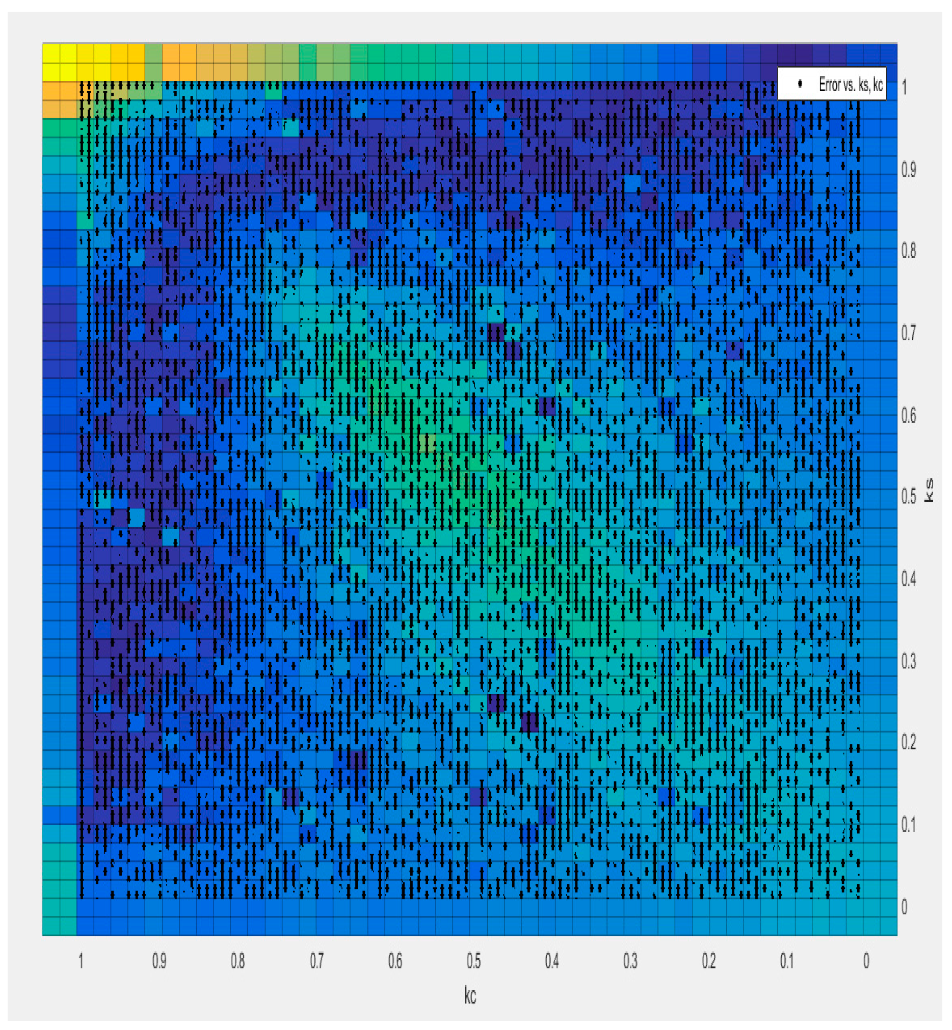
Therefore, we will concentrate on contributing to the economic theory of how the proposed test behaves in different parameter regions by using very extensive parameter regions. This power analysis is primarily designed to shed light on the alleged behavioral pattern in financial markets. The economic events that cause financial markets’ nonlinear convergence behavior are listed as market friction, transaction cost, spread between financial prices, short sales, borrowing restrictions, the interaction of heterogeneous agents, herd behavior, and momentum trading. These economic events make arbitrage unprofitable in small changes and converge to equilibrium for large arbitrages [19]. Therefore, a return to equilibrium only occurs when the deviations from this equilibrium are large, and thus, arbitrage activities are profitable [19]. That is to say, the dynamic behavior of financial variables will differ according to the size of the deviation from equilibrium, regardless of the sign of this deviation. Band TAR and ESTAR functions are available in the literature as functional structures to consider such behaviors.

For this reason, the ESTAR function has been used in many studies to test the exchange rates and PPP hypothesis. Power analysis, which we will discuss below, is primarily designed to compare this behavior at first. The advantages and disadvantages of the proposed test in contrast to other panel unit root tests will be compared. This analysis will be handled when there is a moderate break structure, and how the ESTAR model behaves in high persistence and more nonlinear behavior regions or vice versa will be examined. In order to make comparisons of the proposed new test, initially, the tests closest to the ESTAR convergence containing the logistic trend were selected. The power analysis included in [36] for the panel unit root test considers TAR convergence with a logistics smooth trend. As can be seen, this study is the closest study to the band TAR study mentioned above. In addition, it is the closest test to the proposed test in this study. The sieve bootstrap method was used to eliminate the cross-section dependency as in [33]. Leybourne et al. [18] suggested including intercept and trend test versions when they have not covered any structural break in the UO test. The linear Im, Pesaran, and Shin [39] panel unit root test, which is the initiator of panel unit root tests, was included in the power analysis to compare the parameter regions where linearity increased. Finally, the analysis included the Omay, Hasanov, and Shin [33] panel unit root test with the logistic trend. In this way, all components of the proposed test were also included in the power comparison separately. In their panel unit root test, sieve bootstrap and common correlated error methods were used for remedying cross-section dependency, and it was discussed in detail that the sieve bootstrap method is a better remedy. In light of these explanations, it is clear that if the selected parameters provide high persistence and nonlinearity in power comparison, these parameter regions are the regions where we observe real exchange behavior. When we decrease the high persistence and nonlinearity parameters, the power of the proposed test is expected to decrease and vice versa. Therefore, by using the below data-generating process, we employ an extensive power analysis:

$$y_{it}={\alpha }_{1,i}+{\alpha }_{2,i}{S}_{i,t}\left({\gamma }_i,{\tau }_i\right)+w_{i,t}$$

(17)

$${\widehat{w}}_{it}={\phi }_{2,i}{\widehat{w}}_{i,t-1}\left(1-\mathit{exp}\left[-{\delta }_i{\widehat{w}}_{i,t-1}^2\right]\right)+{\upsilon }_{i,t}$$

(18)

The parameter regions are given in

Table 8. The power comparison of alternative tests.

	${\alpha }_{2,i}=5.0\hspace{1em}\hspace{1em}{\gamma }_i=0.5\hspace{1em}\hspace{1em}{\tau }_i=0.5\hspace{1em}\hspace{1em}{\phi }_{2,i}=-0.1\hspace{1em}\hspace{1em}{\delta }_i=0.01$
T/N	N = 5						N = 25
	${\overline{t}}_{BRNL}$	${\overline{t}}_{NL}$	${\overline{t}}_{IPS}$	${\overline{t}}_{BR}$	${\overline{t}}_{BrTt}$	${\overline{F}}_{BrTF}$	${\overline{t}}_{BRNL}$	${\overline{t}}_{NL}$	${\overline{t}}_{IPS}$	${\overline{t}}_{BR}$	${\overline{t}}_{BrTt}$	${\overline{F}}_{BrTF}$
30	0.082	0.001	0.001	0.035	0.056	0.052	0.148	0.018	0.011	0.108	0.122	0.123
50	0.148	0.018	0.011	0.108	0.122	0.123	0.185	0.022	0.016	0.122	0.131	0.141
70	0.185	0.022	0.016	0.122	0.130	0.134	0.224	0.041	0.018	0.126	0.211	0.223
100	0.224	0.041	0.018	0.136	0.201	0.201	0.297	0.103	0.042	0.153	0.226	0.233
T/N	N = 50						N = 100
	${\overline{t}}_{BRNL}$	${\overline{t}}_{NL}$	${\overline{t}}_{IPS}$	${\overline{t}}_{BR}$	${\overline{t}}_{BrTt}$	${\overline{F}}_{BrTF}$	${\overline{t}}_{BRNL}$	${\overline{t}}_{NL}$	${\overline{t}}_{IPS}$	${\overline{t}}_{BR}$	${\overline{t}}_{BrTt}$	${\overline{F}}_{BrTF}$
30	0.214	0.025	0.021	0.136	0.142	0.159	0.259	0.032	0.026	0.145	0.153	0.177
50	0.222	0.036	0.025	0.146	0.184	0.194	0.283	0.053	0.032	0.151	0.248	0.265
70	0.263	0.063	0.035	0.168	0.241	0.305	0.302	0.079	0.042	0.185	0.267	0.387
100	0.372	0.165	0.062	0.188	0.291	0.332	0.483	0.227	0.084	0.274	0.325	0.431
	${\alpha }_{2,i}=5.0\hspace{1em}\hspace{1em}{\gamma }_i=0.5\hspace{1em}\hspace{1em}{\tau }_i=0.5\hspace{1em}\hspace{1em}{\phi }_{2,i}=-0.1\hspace{1em}\hspace{1em}{\delta }_i=1.0$
T/N	N = 5						N = 25
	${\overline{t}}_{BRNL}$	${\overline{t}}_{NL}$	${\overline{t}}_{IPS}$	${\overline{t}}_{BR}$	${\overline{t}}_{BrTt}$	${\overline{F}}_{BrTF}$	${\overline{t}}_{BRNL}$	${\overline{t}}_{NL}$	${\overline{t}}_{IPS}$	${\overline{t}}_{BR}$	${\overline{t}}_{BrTt}$	${\overline{F}}_{BrTF}$
30	0.299	0.001	0.001	0.194	0.183	0.185	0.397	0.062	0.061	0.385	0.332	0.348
50	0.356	0.002	0.001	0.288	0.254	0.273	0.428	0.107	0.093	0.419	0.361	0.379
70	0.401	0.012	0.011	0.340	0.325	0.336	0.697	0.256	0.257	0.537	0.324	0.384
100	0.451	0.036	0.034	0.398	0.394	0.361	0.951	0.694	0.689	0.898	0.759	0.858
T/N	N = 50						N = 100
	${\overline{t}}_{BRNL}$	${\overline{t}}_{NL}$	${\overline{t}}_{IPS}$	${\overline{t}}_{BR}$	${\overline{t}}_{BrTt}$	${\overline{F}}_{BrTF}$	${\overline{t}}_{BRNL}$	${\overline{t}}_{NL}$	${\overline{t}}_{IPS}$	${\overline{t}}_{BR}$	${\overline{t}}_{BrTt}$	${\overline{F}}_{BrTF}$
30	0.638	0.077	0.068	0.613	0.514	0.512	0.865	0.106	0.071	0.860	0.683	0.847
50	0.647	0.116	0.105	0.631	0.363	0.449	0.898	0.217	0.118	0.872	0.705	0.806
70	0.875	0.417	0.409	0.836	0.474	0.604	0.989	0.718	0.639	0.977	0.711	0.939
100	0.996	0.928	0.923	0.992	0.934	0.946	1.000	0.985	0.980	1.000	0.989	1.000
	${\alpha }_{2,i}=5.0\hspace{1em}\hspace{1em}{\gamma }_i=0.5\hspace{1em}\hspace{1em}{\tau }_i=0.5\hspace{1em}\hspace{1em}{\phi }_{2,i}=-1.0\hspace{1em}\hspace{1em}{\delta }_i=0.01$
T/N	N = 5						N = 25
	${\overline{t}}_{BRNL}$	${\overline{t}}_{NL}$	${\overline{t}}_{IPS}$	${\overline{t}}_{BR}$	${\overline{t}}_{BrTt}$	${\overline{F}}_{BrTF}$	${\overline{t}}_{BRNL}$	${\overline{t}}_{NL}$	${\overline{t}}_{IPS}$	${\overline{t}}_{BR}$	${\overline{t}}_{BrTt}$	${\overline{F}}_{BrTF}$
30	0.301	0.001	0.001	0.238	0.235	0.237	0.566	0.134	0.102	0.474	0.401	0.406
50	0.366	0.005	0.004	0.338	0.332	0.337	0.707	0.344	0.174	0.647	0.422	0.439
70	0.478	0.017	0.015	0.387	0.378	0.385	0.957	0.681	0.426	0.795	0.573	0.648
100	0.718	0.081	0.045	0.488	0.474	0.484	1.000	0.982	0.951	0.986	0.982	0.985
T/N	N = 50						N = 100
	${\overline{t}}_{BRNL}$	${\overline{t}}_{NL}$	${\overline{t}}_{IPS}$	${\overline{t}}_{BR}$	${\overline{t}}_{BrTt}$	${\overline{F}}_{BrTF}$	${\overline{t}}_{BRNL}$	${\overline{t}}_{NL}$	${\overline{t}}_{IPS}$	${\overline{t}}_{BR}$	${\overline{t}}_{BrTt}$	${\overline{F}}_{BrTF}$
30	0.677	0.178	0.168	0.621	0.517	0.543	0.958	0.436	0.151	0.956	0.819	0.927
50	0.898	0.548	0.281	0.862	0.666	0.719	0.997	0.839	0.374	0.992	0.905	0.972
70	0.996	0.909	0.732	0.975	0.834	0.882	0.999	0.997	0.929	0.999	0.963	0.996
100	0.999	0.994	0.986	0.999	0.996	0.997	1.000	1.000	1.000	1.000	1.000	1.000
	${\alpha }_{2,i}=5.0\hspace{1em}\hspace{1em}{\gamma }_i=0.5\hspace{1em}\hspace{1em}{\tau }_i=0.5\hspace{1em}\hspace{1em}{\phi }_{2,i}=-1.0\hspace{1em}\hspace{1em}{\delta }_i=1.0$
T/N	N = 5						N = 25
	${\overline{t}}_{BRNL}$	${\overline{t}}_{NL}$	${\overline{t}}_{IPS}$	${\overline{t}}_{BR}$	${\overline{t}}_{BrTt}$	${\overline{F}}_{BrTF}$	${\overline{t}}_{BRNL}$	${\overline{t}}_{NL}$	${\overline{t}}_{IPS}$	${\overline{t}}_{BR}$	${\overline{t}}_{BrTt}$	${\overline{F}}_{BrTF}$
30	1.000	0.383	0.562	0.999	0.999	1.000	1.000	1.000	1.000	1.000	1.000	1.000
50	1.000	0.972	0.993	1.000	1.000	1.000	1.000	1.000	1.000	1.000	1.000	1.000
70	1.000	0.994	0.998	1.000	1.000	1.000	1.000	1.000	1.000	1.000	1.000	1.000
100	1.000	0.998	0.995	1.000	1.000	1.000	1.000	1.000	1.000	1.000	1.000	1.000
T/N	N = 50						N = 100
	${\overline{t}}_{BRNL}$	${\overline{t}}_{NL}$	${\overline{t}}_{IPS}$	${\overline{t}}_{BR}$	${\overline{t}}_{BrTt}$	${\overline{F}}_{BrTF}$	${\overline{t}}_{BRNL}$	${\overline{t}}_{NL}$	${\overline{t}}_{IPS}$	${\overline{t}}_{BR}$	${\overline{t}}_{BrTt}$	${\overline{F}}_{BrTF}$
30	1.000	1.000	1.000	1.000	1.000	1.000	1.000	1.000	1.000	1.000	1.000	1.000
50	1.000	1.000	1.000	1.000	1.000	1.000	1.000	1.000	1.000	1.000	1.000	1.000
70	1.000	1.000	1.000	1.000	1.000	1.000	1.000	1.000	1.000	1.000	1.000	1.000
100	1.000	1.000	1.000	1.000	1.000	1.000	1.000	1.000	1.000	1.000	1.000	1.000

Note:  ${\overline{t}}_{BRNL}$ indicates the PLSTTESTAR newly proposed test, ${\overline{t}}_{NL}$ is PESTAR UO (2009) test, ${\overline{t}}_{IPS}$ is IPS (2003) test, ${\overline{t}}_{BR}$ is PLSTT OHS (2018) test, and ${\overline{t}}_{BrTt}$ ${\overline{F}}_{BrTF}$ are PLSTTTAR OCE (2018) tests. The Monte Carlo trials are 2000.

. This table is devoted to the ESTAR (1) component of the newly proposed test: state-dependent nonlinear behavior around a nonlinear attractor, namely, a logistic smooth transition trend. Therefore, in the first part of the power analysis, we investigate the financial variable behaviors in high persistence and nonlinearity regions.

As the transition speed parameter delta ${\delta }_i$ in the ESTAR (1) part of the newly proposed test becomes smaller, the power increases in the newly proposed test are greater than the linear models. This situation increases the power of the panel unit root test, independent of other parameters that determine the structure of the test. Kapetanios et al. [19] observed this power relationship between the KSS and ADF tests. Among the panel unit root tests we discussed here, this relationship is similar to that between the proposed and OHS tests (panel logistic smooth transition trend). For example, power analysis results were obtained as 0.224 and 0.136 for N = 5, T = 100, and ${\delta }_i$ = 0.01 values for PLSTTESTAR (1) and PLSTT unit root tests, respectively. Meanwhile, 0.451 and 0.398 were obtained for N = 5, T = 100, and ${\delta }_i$ = 1.0 values. If the ratio of the power result obtained for the new test and the OHS test results is 1.64 times higher when ${\delta }_i$ is small (N = 5, T = 100 and gamma 0.01), it decreases to 1.13 times when ${\delta }_i$ is large (N = 5, T = 100 and gamma 1.0). This relationship is seen in all parameters and N and T combinations. The generated series converges toward a linear process as ${\delta }_i$ grows, so the remaining part in the nonlinear de-trend series becomes linear. In addition, the persistence of the series increases as ${\phi }_{2,i}$ increases. As the transition rate parameter ${\phi }_{2,i}$ in the ESTAR (1) part of the proposed test increases, the power increases more than all other tests. This situation increases the power of the newly proposed panel unit root test, independent of other parameters that determine the structure of the test. Therefore, the proposed test has higher power in more persistent data generation areas. The power analysis reveals that the proposed test captures the financial data’s high persistence and nonlinear characteristics well. Power analysis will be continued within the framework of the economic relationship of the PPP hypothesis with structural breaks. Most empirical studies accepted the PPP hypothesis by using structural break unit root testing.

Regarding this issue, Hegwood and Papell [10] state that a very long data range covers both fixed and floating exchange rate regimes and may produce spurious results due to regime changes. In another example, Edison and Kloveland [44] note that, although the homogeneity assumption behind the standard view of PPP is valid only in the long run, long data streams can encounter regime changes in tastes and technology, which means permanent movements in the equilibrium of exchange rates. However, they stated that if the equilibrium reel exchange rate deviations are permanent, it will cause the quasi-PPP hypothesis.

Nevertheless, they emphasize that the standard PPP will still be valid under the temporary break condition. In addition, various external shocks may cause the equilibrium value of the real exchange rate to change over time and continue at a different equilibrium real exchange rate. For example, the oil price shocks of 1973 and the collapse of the socialist bloc in the 1990s may have altered the equilibrium real exchange rates of oil-importing and transition countries, respectively. Even though these structural changes come with shocks, the changes in the exchange rate take time. Thus, they can be better captured by smooth transition models. This power analysis section will show that the PPP hypothesis can be tested more strongly with the correct structural break test. Hegwood and Papell [10] stated that another crucial structural break model is the model in which the long-term PPP hypothesis remains valid by proposing a temporary structural break instead of the quasi-PPP hypothesis. Sollis [14] modeled the pre-appreciation and post-depreciation periods with a temporary break using the exponential smooth transition trend (ESTT) model. Çorakcı et al. [35] evaluated the ESTT model as a monotone function and criticized the Fourier function used in the article [14]. The main goal of these studies is to determine the long-term PPP hypothesis when there is a temporary break. However, since break structures will be found in a wide variety of structures, they are insufficient to analyze short-term data. For the long-run PPP hypothesis, the sample needs to be very long, and the structural break is expected to cause a temporary change in the exchange rate equilibrium. The validity of the test remains very limited under these restrictive assumptions. The hypothesis of Hegwood and Papell [10] and their follower Sollis [14] that the real exchange rate should have an equal, constant mean before and after the structural change is a very limiting hypothesis compared with the quasi-PPP hypothesis. The logistic smooth transition model C we use can capture such structures, albeit partially, and shows whether the long-term PPP hypothesis is valid or not. In this respect, additional information on this subject will be given in the empirical part. In the power analysis section, we will examine the power performances of our test by comparing it with some other tests for different logistic smooth transition parameters.

There are three parameters of the logistic smooth transition trend. The first of these parameters, the ${\alpha }_{2,i}$ parameter, determines the magnitude of the structural break; the transition speed ${\gamma }_i$ parameter determines the speed of the transition from one real exchange rate equilibrium to the next (it determines the duration); and, finally, the threshold ${\tau }_i$ parameter determines the location of the structural break. Smooth, moderate, and sharp breaks can be obtained from combinations of these three parameters. In addition, the permanent break can be obtained with the LST trend, and the model C structure has the flexibility to imitate the temporary break structure. As we mentioned above, the quasi- PPP hypothesis is a more general hypothesis that reveals the superiority of the LSTT function in testing this hypothesis. We mentioned that smooth-transition breaks have better test properties than instant structural breaks because heterogeneous agents cannot take action simultaneously in financial markets. Therefore, this structure leads to a smooth or rather long-duration break structure. In the LSTT function, this feature is provided by the transition speed parameter ${\gamma }_i$. As shown in

Table 9. The power comparison of alternative tests.

	${\alpha }_{2,i}=5.0\hspace{1em}\hspace{1em}{\gamma }_i=0.5\hspace{1em}\hspace{1em}{\tau }_i=0.5\hspace{1em}\hspace{1em}{\phi }_{2,i}=-1.0\hspace{1em}\hspace{1em}{\delta }_i=1.0$
T\N	N = 5						N = 25
	${\overline{t}}_{BRNL}$	${\overline{t}}_{NL}$	${\overline{t}}_{IPS}$	${\overline{t}}_{BR}$	${\overline{t}}_{BrTt}$	${\overline{F}}_{BrTF}$	${\overline{t}}_{BRNL}$	${\overline{t}}_{NL}$	${\overline{t}}_{IPS}$	${\overline{t}}_{BR}$	${\overline{t}}_{BrTt}$	${\overline{F}}_{BrTF}$
30	0.065	0.008	0.005	0.053	0.053	0.048	0.147	0.107	0.101	0.141	0.129	0.111
50	0.088	0.009	0.007	0.082	0.083	0.079	0.194	0.118	0.111	0.158	0.149	0.122
70	0.095	0.014	0.008	0.088	0.086	0.082	0.380	0.190	0.181	0.274	0.242	0.193
100	0.143	0.054	0.026	0.149	0.118	0.104	0.807	0.345	0.338	0.532	0.359	0.349
T\N	N = 50						N = 100
	${\overline{t}}_{BRNL}$	${\overline{t}}_{NL}$	${\overline{t}}_{IPS}$	${\overline{t}}_{BR}$	${\overline{t}}_{BrTt}$	${\overline{F}}_{BrTF}$	${\overline{t}}_{BRNL}$	${\overline{t}}_{NL}$	${\overline{t}}_{IPS}$	${\overline{t}}_{BR}$	${\overline{t}}_{BrTt}$	${\overline{F}}_{BrTF}$
30	0.185	0.120	0.119	0.145	0.138	0.121	0.241	0.186	0.179	0.219	0.216	0.205
50	0.199	0.154	0.151	0.197	0.184	0.175	0.298	0.201	0.198	0.285	0.262	0.258
70	0.404	0.224	0.219	0.396	0.387	0.239	0.578	0.326	0.322	0.557	0.406	0.401
100	0.863	0.505	0.502	0.848	0.562	0.551	0.989	0.697	0.692	0.979	0.724	0.954
	${\alpha }_{2,i}=5.0\hspace{1em}\hspace{1em}{\gamma }_i=5.0\hspace{1em}\hspace{1em}{\tau }_i=0.5\hspace{1em}\hspace{1em}{\phi }_{2,i}=-0.1\hspace{1em}\hspace{1em}{\delta }_i=1.0$
T\N	N = 5						N = 25
	${\overline{t}}_{BRNL}$	${\overline{t}}_{NL}$	${\overline{t}}_{IPS}$	${\overline{t}}_{BR}$	${\overline{t}}_{BrTt}$	${\overline{F}}_{BrTF}$	${\overline{t}}_{BRNL}$	${\overline{t}}_{NL}$	${\overline{t}}_{IPS}$	${\overline{t}}_{BR}$	${\overline{t}}_{BrTt}$	${\overline{F}}_{BrTF}$
30	0.109	0.005	0.001	0.081	0.021	0.024	0.127	0.009	0.003	0.098	0.025	0.035
50	0.132	0.010	0.005	0.102	0.072	0.085	0.249	0.029	0.025	0.117	0.080	0.098
70	0.146	0.015	0.010	0.117	0.065	0.079	0.772	0.417	0.402	0.574	0.479	0.505
100	0.239	0.027	0.021	0.232	0.138	0.158	0.957	0.645	0.633	0.806	0.716	0.791
T\N	N = 50						N = 100
	${\overline{t}}_{BRNL}$	${\overline{t}}_{NL}$	${\overline{t}}_{IPS}$	${\overline{t}}_{BR}$	${\overline{t}}_{BrTt}$	${\overline{F}}_{BrTF}$	${\overline{t}}_{BRNL}$	${\overline{t}}_{NL}$	${\overline{t}}_{IPS}$	${\overline{t}}_{BR}$	${\overline{t}}_{BrTt}$	${\overline{F}}_{BrTF}$
30	0.181	0.011	0.005	0.109	0.044	0.048	0.262	0.014	0.009	0.130	0.063	0.073
50	0.434	0.039	0.031	0.164	0.149	0.155	0.671	0.051	0.039	0.252	0.218	0.236
70	0.798	0.428	0.424	0.552	0.518	0.536	0.963	0.621	0.612	0.848	0.713	0.798
100	0.971	0.914	0.905	0.992	0.741	0.844	1.000	0.996	0.992	1.000	0.998	1.000
	${\alpha }_{2,i}=5.0\hspace{1em}\hspace{1em}{\gamma }_i=5.0\hspace{1em}\hspace{1em}{\tau }_i=0.2\hspace{1em}\hspace{1em}{\phi }_{2,i}=-0.1\hspace{1em}\hspace{1em}{\delta }_i=1.0$
T\N	N = 5						N = 25
	${\overline{t}}_{BRNL}$	${\overline{t}}_{NL}$	${\overline{t}}_{IPS}$	${\overline{t}}_{BR}$	${\overline{t}}_{BrTt}$	${\overline{F}}_{BrTF}$	${\overline{t}}_{BRNL}$	${\overline{t}}_{NL}$	${\overline{t}}_{IPS}$	${\overline{t}}_{BR}$	${\overline{t}}_{BrTt}$	${\overline{F}}_{BrTF}$
30	0.032	0.005	0.002	0.006	0.009	0.007	0.058	0.024	0.022	0.028	0.037	0.033
50	0.059	0.017	0.010	0.019	0.018	0.029	0.085	0.042	0.040	0.045	0.055	0.052
70	0.081	0.053	0.024	0.055	0.064	0.062	0.380	0.270	0.255	0.278	0.289	0.284
100	0.147	0.123	0.064	0.128	0.132	0.130	0.813	0.710	0.701	0.718	0.725	0.722
T\N	N = 50						N = 100
	${\overline{t}}_{BRNL}$	${\overline{t}}_{NL}$	${\overline{t}}_{IPS}$	${\overline{t}}_{BR}$	${\overline{t}}_{BrTt}$	${\overline{F}}_{BrTF}$	${\overline{t}}_{BRNL}$	${\overline{t}}_{NL}$	${\overline{t}}_{IPS}$	${\overline{t}}_{BR}$	${\overline{t}}_{BrTt}$	${\overline{F}}_{BrTF}$
30	0.078	0.035	0.033	0.058	0.067	0.063	0.078	0.035	0.033	0.058	0.067	0.063
50	0.177	0.151	0.148	0.165	0.175	0.171	0.177	0.151	0.148	0.165	0.175	0.171
70	0.468	0.377	0.356	0.395	0.401	0.399	0.468	0.377	0.356	0.395	0.401	0.399
100	0.898	0.824	0.820	0.856	0.868	0.865	0.978	0.911	0.901	0.946	0.958	0.956
	${\alpha }_{2,i}=10.0\hspace{1em}\hspace{1em}{\gamma }_i=5.0\hspace{1em}\hspace{1em}{\tau }_i=0.5\hspace{1em}\hspace{1em}{\phi }_{2,i}=-0.1\hspace{1em}\hspace{1em}{\delta }_i=1.0$
T\N	N = 5						N = 25
	${\overline{t}}_{BRNL}$	${\overline{t}}_{NL}$	${\overline{t}}_{IPS}$	${\overline{t}}_{BR}$	${\overline{t}}_{BrTt}$	${\overline{F}}_{BrTF}$	${\overline{t}}_{BRNL}$	${\overline{t}}_{NL}$	${\overline{t}}_{IPS}$	${\overline{t}}_{BR}$	${\overline{t}}_{BrTt}$	${\overline{F}}_{BrTF}$
30	0.138	0.000	0.000	0.024	0.026	0.023	0.144	0.000	0.000	0.056	0.059	0.046
50	0.149	0.000	0.000	0.029	0.038	0.034	0.245	0.030	0.000	0.114	0.124	0.111
70	0.197	0.000	0.000	0.081	0.085	0.079	0.817	0.062	0.000	0.306	0.326	0.302
100	0.238	0.019	0.000	0.220	0.225	0.201	0.986	0.098	0.000	0.724	0.729	0.721
T\N	N = 50						N = 100
	${\overline{t}}_{BRNL}$	${\overline{t}}_{NL}$	${\overline{t}}_{IPS}$	${\overline{t}}_{BR}$	${\overline{t}}_{BrTt}$	${\overline{F}}_{BrTF}$	${\overline{t}}_{BRNL}$	${\overline{t}}_{NL}$	${\overline{t}}_{IPS}$	${\overline{t}}_{BR}$	${\overline{t}}_{BrTt}$	${\overline{F}}_{BrTF}$
30	0.185	0.009	0.000	0.086	0.089	0.085	0.294	0.028	0.001	0.178	0.198	0.177
50	0.599	0.056	0.000	0.217	0.221	0.216	0.819	0.076	0.005	0.305	0.316	0.304
70	0.879	0.083	0.000	0.506	0.511	0.504	0.984	0.124	0.011	0.722	0.734	0.730
100	0.996	0.102	0.000	0.815	0.823	0.814	1.000	0.206	0.017	0.933	0.936	0.932

Note: ${\overline{t}}_{BRNL}$ indicates the PLSTTESTAR newly proposed test, ${\overline{t}}_{NL}$ is PESTAR UO (2009) test, ${\overline{t}}_{IPS}$ is IPS (2003) test, ${\overline{t}}_{BR}$ is PLSTT OHS (2018) test, and ${\overline{t}}_{BrTt}$ and ${\overline{F}}_{BrTF}$ are PLSTTTAR OCE (2018) tests. The Monte Carlo trials are 2000.

, the power of unit root tests with the LSTT function increases as the transition speed parameter ${\gamma }_i$ becomes smaller. In addition, as the size of the break parameter ${\alpha }_{2,i}$ increases, the power performance of the tests with the LSTT function increases, compared with the tests without structural breaks. Another interesting result is that while the structural break parameters approach the middle of the sample, the power performance of panel unit root tests, including LSTT, increases. In the Table 9, we consider three different cases depending on the magnitudes of the structural break parameter ${\alpha }_{2,i}$. For the small or moderate break with ${\alpha }_{2,i}$ = 5.0, the IPS or any other panel unit root test without any structural component has better power features than higher structural break parameters. See also similar results documented in Leybourne et al. [18], Sollis [14], and Omay and Yıldırım [20]. The power of all the tests is negatively associated with the ${\gamma }_i$ parameter. Furthermore, the threshold location parameter, ${\tau }_i$, also negatively affects the power of the smooth transition-type tests. In particular, when the threshold is located at the beginning of the sample, LST trend unit root tests tend to display lower power performance with respect to ${\tau }_i$ = 0.5. As expected, in all of the parameter region, the panel LSTTESTAR (1) test becomes more powerful than the other tests in which the ESTAR (1) parameter is selected to imitate the high persistency and nonlinear structure of financial markets. Hence, we may conclude that the logistic smooth transition function can capture the small, moderate, and sharper breaks. Finally, when the structural break parameter is substantially large, the IPS and UO tests lose power. The performance of the smooth transition-type de-trending tests improves when the value of the structural break parameter increases. Therefore, the panel LSTTESTAR (1), PLSTT, and panel threshold autoregressive with logistic smooth transition trend (i.e PLSTTTAR) test should become more powerful in this region. Therefore, the PLSTTESTAR (1) test outperforms other tests for the cases with moderate, high structural breaks and high transition speeds with the threshold located in the middle. The unit root test procedures proposed in this article have excellent features compatible with the theoretical and empirical dynamics of many economic time series, including real exchange rates. The proposed tests allow for permanent and temporary structural breaks, whereas shifts between regimes might be relatively gradual.

4. Cross-Section Dependency (CSD)

A generally faced problem in panel regression models is the presence of CSD. CSD can arise because of spatial correlations, spill-over effects, economic distance, omitted global variables, and common unobserved shocks. Correlated errors through individuals make the classical unit root and cointegration testing procedure invalid in panel data models. Banerjee et al. [22] assess the finite sample performance of the available tests and find that all tests experience severe size distortions when panel members are cointegrated. To overcome this issue, some tests based on the regression equation, including the unobserved or observed factors as the additional regressors, have been suggested in recent years (e.g., [23,24,25,41,45,46]).

On the other hand, Maddala and Wu [27], Chang [28], and Ucar and Omay [31] consider the bootstrap-based tests to obtain good size properties. In this study, we used two methods to deal with the cross-section dependency problem. One is the common correlated effect (henceforth, CCE) estimator proposed by Pesaran [25], and the other is the bootstrap method. In the bootstrap method, we impose the methodology of the UO test.

The CCE estimation procedure has the advantage that the least number of squares can compute it to auxiliary regression, where the observed regressors are augmented with cross-sectional averages of the dependent variable, individual-specific regressors, and state-dependent variables. This augmentation leads to a new set of estimators mentioned in Pesaran (2006), referred to as the common correlated effects (CCE) estimators, that can be computed by running smooth transition panel regressions augmented with cross-section averages of the dependent and independent variables. The CCE procedure applies to panels with single or multiple unobserved factors so long as the number of unobserved factors is fixed.

Let ${\widehat{w}}_{i,t}$ be a panel exponential smooth transition autoregressive process de-trended by the logistic smooth transition trend of order 1 (PESTAR (1)) on the time domain t = 1, 2, …, T for the cross-section units i = 1, 2, …, N. Consider ${\widehat{w}}_{i,t}$ generated by the following PESTAR (1) process:

$$\Delta {\widehat{w}}_{it}={\phi }_{1,i}{\widehat{w}}_{i,t-1}+{\phi }_{2,i}{\widehat{w}}_{i,t-1}\left(1-\mathit{exp}\left[-{\delta }_i{\widehat{w}}_{i,t-1}^2\right]\right)+{\upsilon }_{i,t}$$

(19)

where $d=1$ is the delay parameter and ${\delta }_i\ge 0$ represents the speed of transition for all units, and ${\upsilon }_{i,t}$ is a serially and cross-sectionally uncorrelated disturbance term with zero mean and variance ${\sigma }_i^2$.

By considering the previous literature, Ucar and Omay [31] set ${\phi }_{1,i}=0$ for all i and $d=1$, which gives the specific PESTAR (1) model:

$$\Delta {\widehat{w}}_{it}={\phi }_{2,i}{\widehat{w}}_{i,t-1}\left(1-\mathit{exp}\left[-{\delta }_i{\widehat{w}}_{i,t-1}^2\right]\right)+{\upsilon }_{i,t}$$

(20)

A nonlinear panel data unit root based on regression (19) with augmented lag variables in empirical application is simply to test the null hypothesis ${\delta }_i=0$ for all i against ${\delta }_i\ge 0$ for some i under the alternative.

However, directly testing the null is problematic since ${\delta }_i$ is not identified under the null. This problem can be solved by taking first-order Taylor series expansion to the PESTAR (1) model around ${\delta }_i=0$ for all i. Hence, the obtained auxiliary regression is given by:

$$\Delta {\widehat{w}}_{i,t}={\rho }_i{\widehat{w}}_{i,t-1}^3+{\sum }_{j=1}^k{\delta }_{i,j}\Delta {\widehat{w}}_{i,t-j}+{\widehat{\eta }}_{i,t}$$

(21)

In empirical application, Equation (18) was augmented by lagged variables of a dependent variable by using Akaike information criteria (AIC) and Schwarz–Bayesian information criteria (SBC). Now, if we include the factor structure into the nonlinear model with a single factor:

$$\Delta {\widehat{w}}_{i,t}={\rho }_i{\widehat{w}}_{i,t-1}^3+{\eta }_{i,t}$$

(22)

$${\eta }_{i,t}={\lambda }_i{f}_t+u_{i,t}$$

(23)

$$u_{i,t}\sim iid.N\left(0,{\sigma }_i^2\right), \mathrm{and} f_t\sim N\left(0,{\sigma }_f^2\right)$$

(24)

Notice here that $f_t$ is the unobserved common factor, ${\lambda }_i$ are the factor loadings, and $u_{i,t}$s are idiosyncratic error terms assumed to be independently distributed across i and t. Note that ${\widehat{w}}_{i,t}$ are de-trended series from Equations (8)–(10). Thus, following the article of Pesaran [25], we obtain the below auxiliary regression for approximating the unobserved factors:

$$\Delta {\widehat{w}}_{i,t}={\rho }_i{\widehat{w}}_{i,t-1}^3+{\Phi }_i{\overline{\widehat{w}}}_{t-1}^3+{\iota }_i{\overline{\Delta \widehat{w}}}_t+{\eta }_{i,t}$$

(25)

Now we can obtain the critical values by using this transformation to eliminate cross-section dependency for the statistic:

$${\overline{t}}_{BRNL,j}^{CCE}=N^{-1}{\sum }_{i=1}^N{t}_{i,BRNL}^{CCE}\hspace{1em}\hspace{1em}j=\left\{A,B,C\right\}$$

(26)

Table 10. Exact critical values of ${\overline{t}}_{BRNL,A}^{CCE}$ statistics model A under CSD.

T\N	5	10	15	20	25	50	100
	1%
30	−3.426	−3.071	−2.955	−2.888	−2.843	−2.731	−2.659
50	−3.420	−3.051	−2.952	−2.882	−2.829	−2.728	−2.655
70	−3.346	−3.042	−2.950	−2.879	−2.817	−2.726	−2.653
100	−3.296	−3.028	−2.943	−2.873	−2.812	−2.725	−2.636
	5%
30	−3.033	−2.854	−2.797	−2.736	−2.709	−2.635	−2.577
50	−3.018	−2.848	−2.782	−2.729	−2.699	−2.630	−2.560
70	−3.017	−2.844	−2.777	−2.724	−2.694	−2.629	−2.550
100	−3.015	−2.839	−2.770	−2.716	−2.689	−2.626	−2.548
	10%
30	−2.879	−2.751	−2.700	−2.666	−2.650	−2.586	−2.577
50	−2.864	−2.743	−2.698	−2.659	−2.635	−2.581	−2.534
70	−2.860	−2.712	−2.690	−2.655	−2.627	−2.578	−2.556
100	−2.853	−2.703	−2.687	−2.652	−2.621	−2.576	−2.551

,

Table 11. Exact critical values of ${\overline{t}}_{BRNL,B}^{CCE}$ statistics model B under CSD.

T\N	5	10	15	20	25	50	100
				1%
30	−3.882	−3.577	−3.491	−3.448	−3.369	−3.208	−3.170
50	−3.863	−3.496	−3.374	−3.295	−3.251	−3.183	−3.090
70	−3.832	−3.416	−3.369	−3.271	−3.212	−3.123	−3.056
100	−3.730	−3.447	−3.356	−3.249	−3.248	−3.118	−3.056
				5%
30	−3.588	−3.366	−3.285	−3.229	−3.214	−3.121	−3.075
50	−3.498	−3.301	−3.189	−3.152	−3.134	−3.069	−3.007
70	−3.466	−3.249	−3.186	−3.146	−3.119	−3.059	−3.007
100	−3.426	−3.242	−3.178	−3.141	−3.118	−3.050	−3.000
				10%
30	−3.384	−3.260	−3.196	−3.152	−3.139	−3.073	−3.035
50	−3.326	−3.186	−3.109	−3.078	−3.076	−3.015	−2.981
70	−3.294	−3.158	−3.094	−3.077	−3.058	−3.011	−2.973
100	−3.291	−3.136	−3.025	−3.076	−3.058	−3.010	−2.973

and

Table 12. Exact critical values of ${\overline{t}}_{BRNL,C}^{CCE}$ statistics model C under CSD.

T\N	5	10	15	20	25	50	100
				1%
30	−4.102	−3.852	−3.691	−3.627	−3.556	−3.449	−3.320
50	−4.043	−3.745	−3.613	−3.499	−3.458	−3.331	−3.228
70	−3.945	−3.636	−3.544	−3.479	−3.424	−3.329	−3.198
100	−3.875	−3.612	−3.509	−3.457	−3.399	−3.217	−3.108
				5%
30	−3.664	−3.592	−3.521	−3.455	−3.416	−3.352	−3.296
50	−3.656	−3.493	−3.430	−3.375	−3.336	−3.264	−3.210
70	−3.590	−3.434	−3.378	−3.345	−3.302	−3.234	−3.152
100	−3.517	−3.426	−3.348	−3.320	−3.281	−3.192	−3.081
				10%
30	−3.497	−3.479	−3.412	−3.366	−3.342	−3.298	−3.256
50	−3.486	−3.378	−3.332	−3.295	−3.266	−3.217	−3.182
70	−3.457	−3.323	−3.287	−3.256	−3.237	−3.192	−3.124
100	−3.427	−3.316	−3.269	−3.243	−3.215	−3.178	−3.001

provide the critical values for different models since the true DGP is generated with cross sectionally dependent data.

In this paper, we also examine the UO test and hence apply the sieve bootstrap method to deal with the cross-section dependency problem. Note that ${\widehat{w}}_{i,t}$ are de-trended series from Equations (8)–(10); therefore, the deterministic term ${\varphi }_i\left(t\right)$ is also included in our computations.

• The following OLS regression is considered for each entity, which allows for different lag orders  $p_i$

  $$\Delta {\widehat{w}}_{i,t}={\rho }_i{\widehat{w}}_{i,t-1}^3+{\sum }_{j=1}^{p_i}{\psi }_{i,j}\Delta {\widehat{w}}_{i,t-j}+{\eta }_{i,t}$$

  (27)
• The null of no unit root is imposed to generate samples of residuals. Errors are estimated as below:

  $${\widehat{\eta }}_{i,t}=\Delta {\widehat{w}}_{i,t}-{\sum }_{j=1}^{p_i}{\varpi }_{i,j}\Delta {\widehat{w}}_{i,t-j}$$

  (28)
• Stine (1987) offers that the residuals have to be centered with

  $${\tilde{\eta }}_t={\widehat{\eta }}_t-\frac{1}{\left(T-p-2\right)}{\sum }_{t=p+2}^T{\widehat{\eta }}_t$$

  (29)

  where ${\widehat{\eta }}_t=({\widehat{\eta }}_{1,t},{\widehat{\eta }}_{2,t},\dots ,{\widehat{\eta }}_{N,t}{)}^{\prime }$ and $p=\underset{i}{max}\left(p_i\right)$. Moreover, we construct the $NxT\left[{\tilde{\eta }}_{i,t}\right]$ matrix from these residuals. We select the residuals column randomly with replacement at a time to preserve the cross-section structure of the errors. The bootstrap residuals are denoted as ${\tilde{\eta }}_{i,t}^{*}$, where $t=1,2,\dots .,T^{*}$ and $T^{*}=2T$.
• We first generate stationary bootstrap samples  $\Delta {\widehat{w}}_{i,t}^{*}$ recursively from

  $$\Delta {\widehat{w}}_{i,t}^{*}={\sum }_{j=1}^{p_i}{\kappa }_{i,j}\Delta {\widehat{w}}_{i,t-j}^{*}+{\tilde{\eta }}_{i,t}^{*}$$

  (30)

  where the initial values of $\Delta w_{i,t-j}^{*}$ are set to zero. We then generate $w_{i,t}^{*}$ as the partial sum process

  $${\widehat{w}}_{i,t}^{*}={\sum }_{k=1}^t\Delta {\widehat{w}}_{i,k}^{*}$$

  (31)

The bootstrap statistics ${\overline{t}}_{BRNL,j}^{*}$   $j=\left\{A,B,C\right\}$ are computed for each bootstrap replication by running the regression equation

$$\Delta {\widehat{w}}_{i,t}^{*}={\rho }_i{{\widehat{w}}^3}_{i,t-1}^{*}+\sum _{j=1}^{p_i}{\vartheta }_{i,j}\Delta {\widehat{w}}_{i,t-j}^{*}+v_{i,t}$$

(32)

The empirical distribution of these statistics is produced through 2000 replications. Thus, their p-values are generated using this methodology.

5. Empirical Application

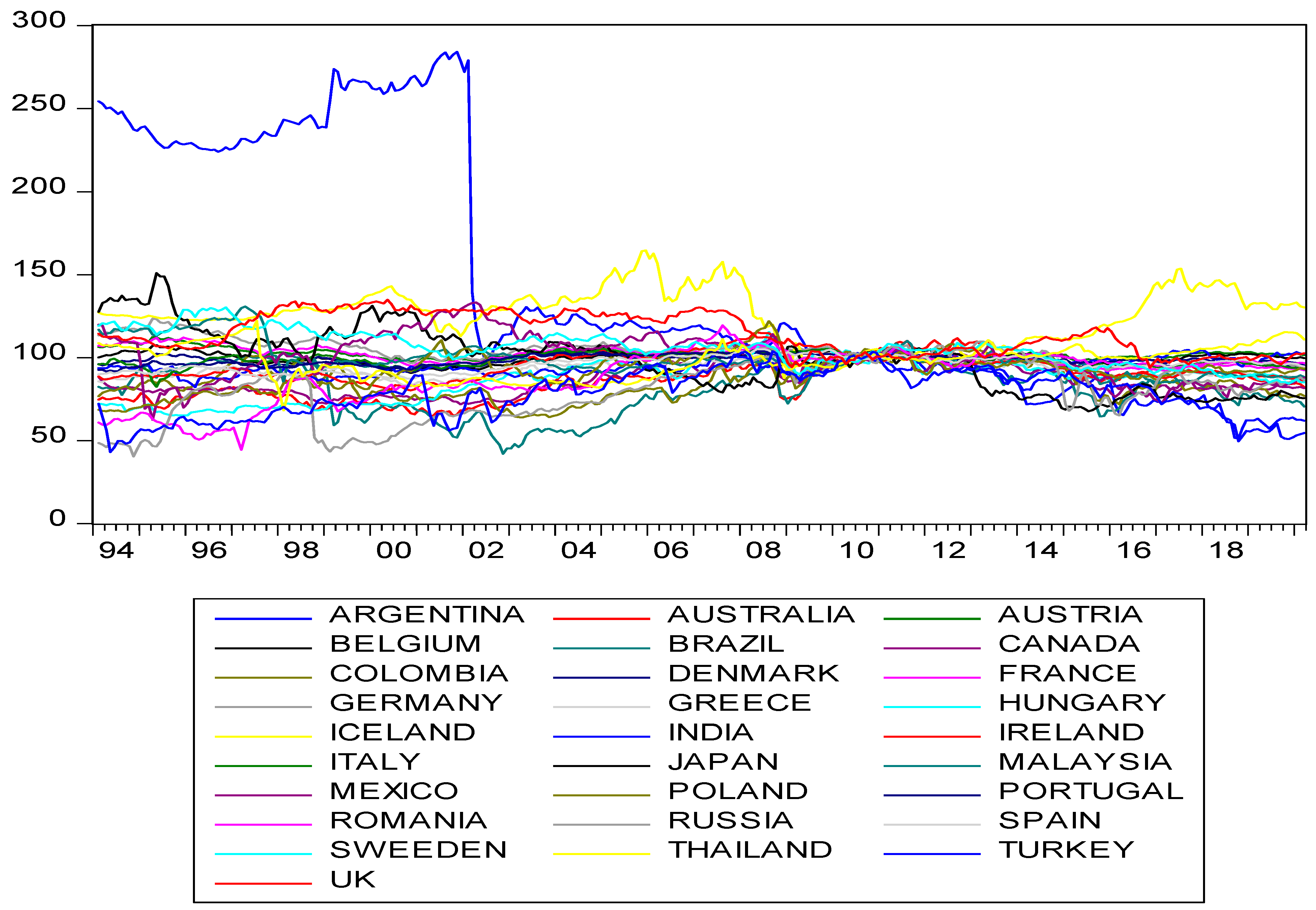
In this study, we selected European and worldwide countries to represent the categories of developed and developing countries. The 34 countries selected are as follows: Argentina, Australia, Austria, Belgium, Brazil, Canada, Colombia, Denmark, France, Germany, Greece, Hungary, Iceland, India, Ireland, Italy, Japan, Malaysia, Mexico, Netherlands, New Zealand, Poland, Portugal, Romania, Russia, Saudi Arabia, South Korea, Slovakia, Spain, Sweden, Switzerland, Thailand, Turkey, and the UK, covering the period 2010:7–2020:3 for the short T panel and 1994:1–2020:3 for the long T panel. Our primary concern in this section is to assess the unit root features of the European and selected representative countries’ real exchange rate, thereby, the PPP hypothesis.

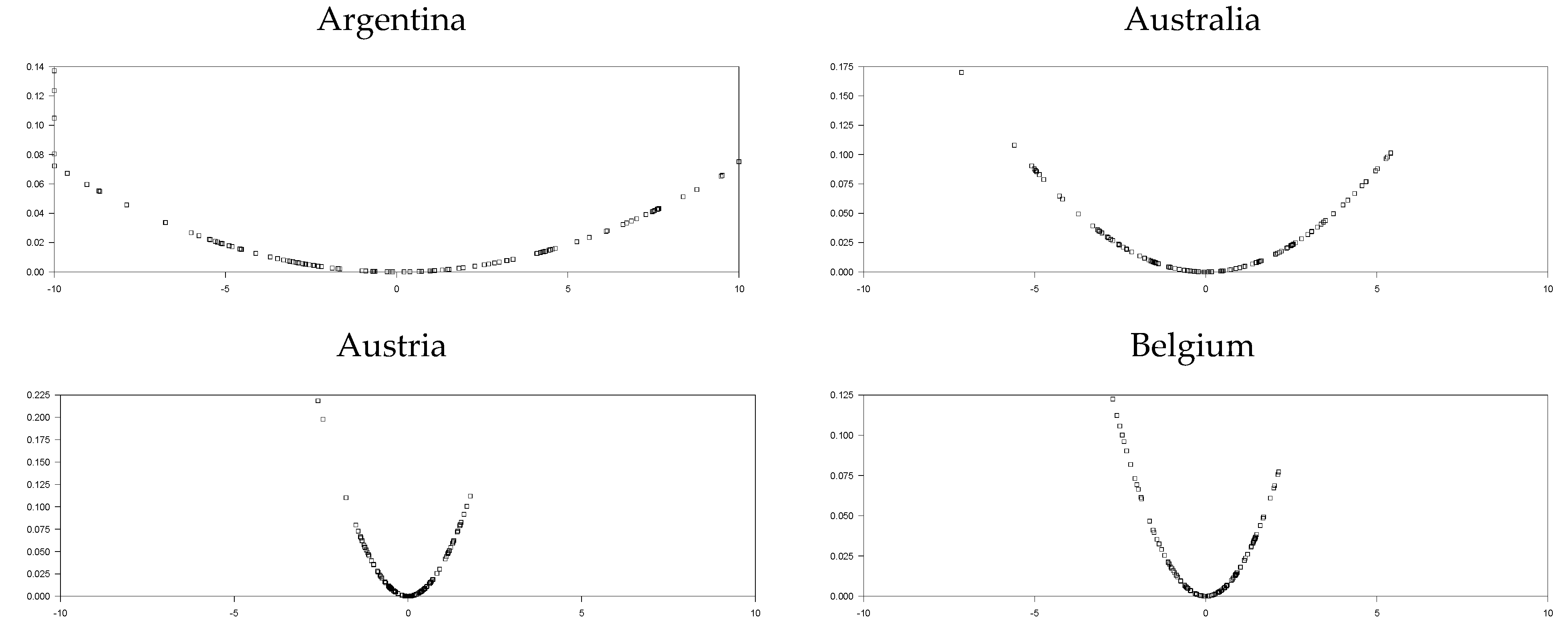
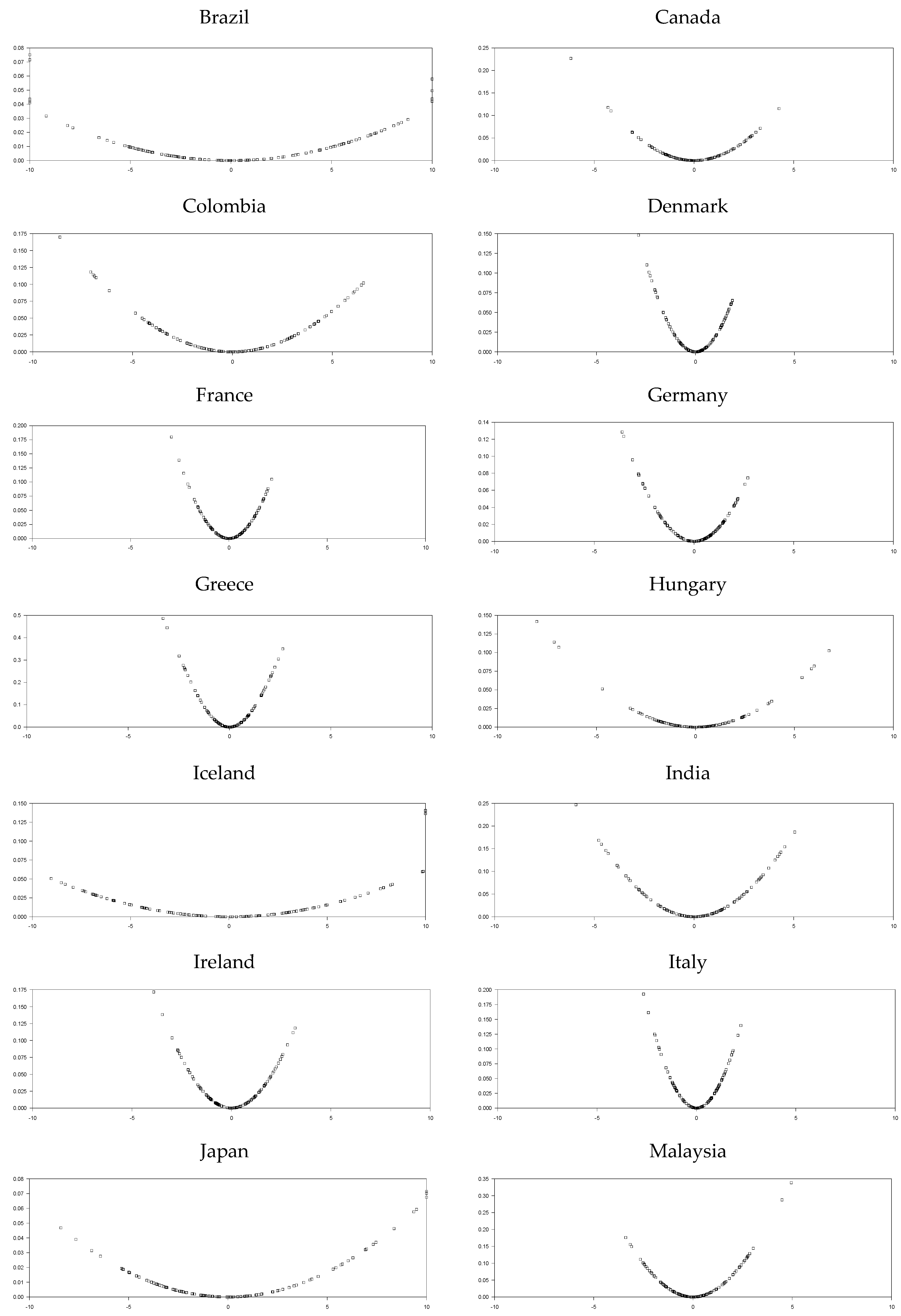
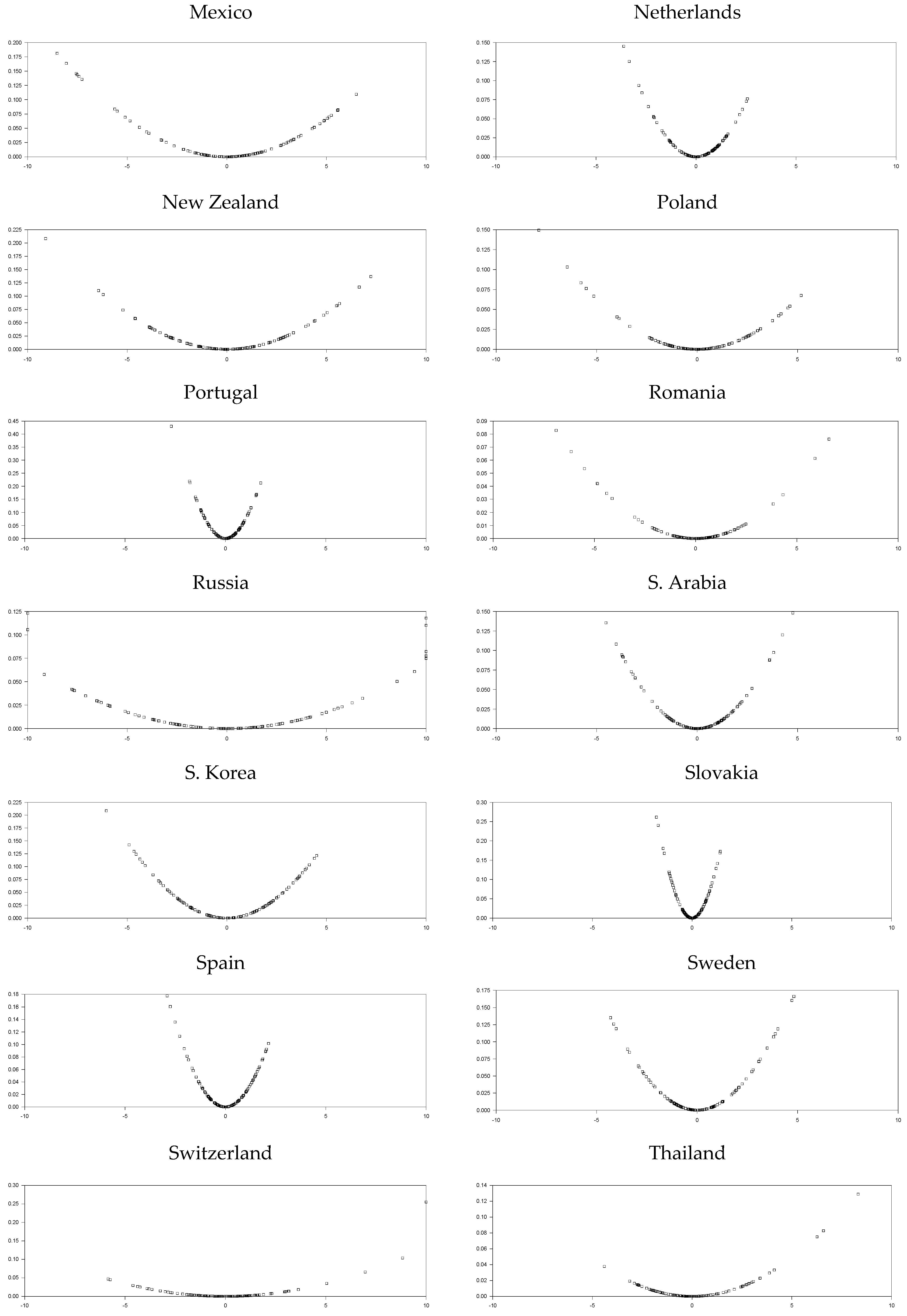
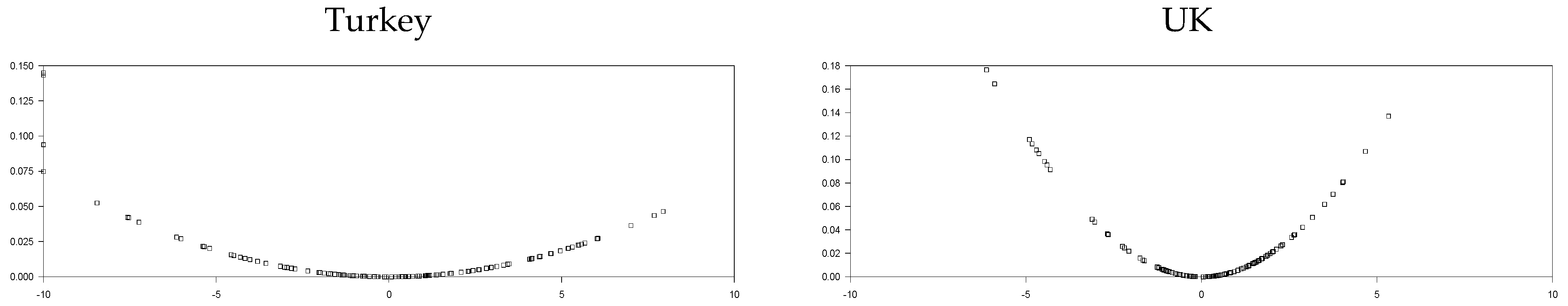
The base year is 2010, which is obviously depicted from Figure 1. We used the sample period of 2010:7–2020:3 in order to remove the base year effect for the short T panel. In the empirical part of the study, we will use different types of panel unit root tests. In addition to the tests we employ in the power analysis section, other panel unit root tests already recommended in the literature will better reveal the REER series structure. In addition to the test we proposed in this study, we will make some comparisons using EO, UO, IPS, OHS, and OCE tests. The EO test does not use the CCE estimator for remedying cross-section dependency. In addition, as stated in Omay et al. [33] (OHS), the CCE estimator catches structural breaks if there are homogeneous structural breaks. In short, it captures the structural break instead of correcting the cross-section dependency. The problem of incorrect decomposition in this estimator (CCE) will lead to difficulties in interpreting the results. Ultimately, a test without a structural break will work as a test with a structural break, giving us false information about the real exchange rate series under consideration. For these reasons, we will compare the results of tests using the sieve bootstrap method in the empirical part to control the cross-section dependency problem.

As can be seen from

Table 13. Panel unit root test results for short T panel: 2010:1–2020:3.

	Intercept	Intercept and Trend
IPS (Linear)	−1.596 (0.572)	−2.477 (0.299)
UO (ESTAR (1))	−2.284 (0.043)	−2.700 (0.047)
EO (AESTAR (1))	3.539 (0.079)	4.670 (0.063)
	Model A	Model B	Model C
OHS (PLSTT)	−3.444 (0.022)	−3.725 (0.102)	−4.014 (0.021)
OCE (PLSTT_TAR)	6.471 (0.065)	7.198 (0.150)	8.832 (0.000)
PLSTT_ESTAR	−3.526 (0.000)	−3.742 (0.000)	−3.837 (0.000)

Note: The p-values are obtained with 2000 bootstrap draws.

, all tests accepted the PPP hypothesis except for the linear sieve bootstrap IPS test. However, it is not known from these results which countries cause significant stationarity. For this reason, it is necessary to understand which test captures the dynamics of the real exchange rate series more meaningfully and differentiates the countries as stationary and nonstationary. Abuaf and Jorion [47], Frankel and Rose [48], Oh [49], Wu [50], and Papell [51], among others, used panel data to increase the number of observations and, thus, the power of the unit root tests. However, Taylor [3] pointed out that conventional panel unit root tests do not provide explicit guidance on the identity of the stationary panel members. They argue that rejecting the null hypothesis of a unit root in panel data implies that at least one of the series is mean reverting but not that all the series under consideration are stationary. In addition, testing stationarity in panels may be complicated by cross-sectional correlation and possible cross-unit cointegration. It is now well established that ignoring cross-sectional correlation or cross-unit cointegration may lead to severe size and power distortions, invalidating inferences drawn from panel tests [52]. In time-series unit root tests, which will be considered individually, common shocks or spillover effects can be seen as structural breaks or nonlinear data generation processes, since they do not control cross-section dependency. Therefore, time-series analysis poses a problem due to this cross-section dependency, which is not controlled by the real exchange rate dynamics.

To consider the cross-section dependency problem, we will continue the empirical part by combining the sequential panel selection method (SPSM) suggested by Chortareas and Kapetanios [53] for our sieve bootstrap estimation. If the panel unit root test finds the full sample stationary, we can continue with SPSM. First, we applied the SPSM method to the tests without a break. Since the sieve bootstrap IPS test without a break in the test procedure did not have a stationary, the SPS method was abandoned, and it was concluded that it did not accept the PPP hypothesis. Fortunately, state-dependent tests were stationary in the full sample for only intercept, intercept, and trend cases. For the validity of the PPP hypothesis, the intercept-only case is consistent with the theory; hence, we continue SPSM with the intercept-only case. As seen from the UO test, only the test, including the intercept, gave more significant results than the intercept and trend case. Selecting a more significant test value for the SPS methodology will increase the number of stationary countries obtained. However, we considered it appropriate to include the SPS methodology to test structures following economic theory rather than statistical significance. Therefore, while the intercept and trend form of the EO test is more significant than the intercept-only case, we performed SPSM by considering the case with intercept-only, as we explained above.

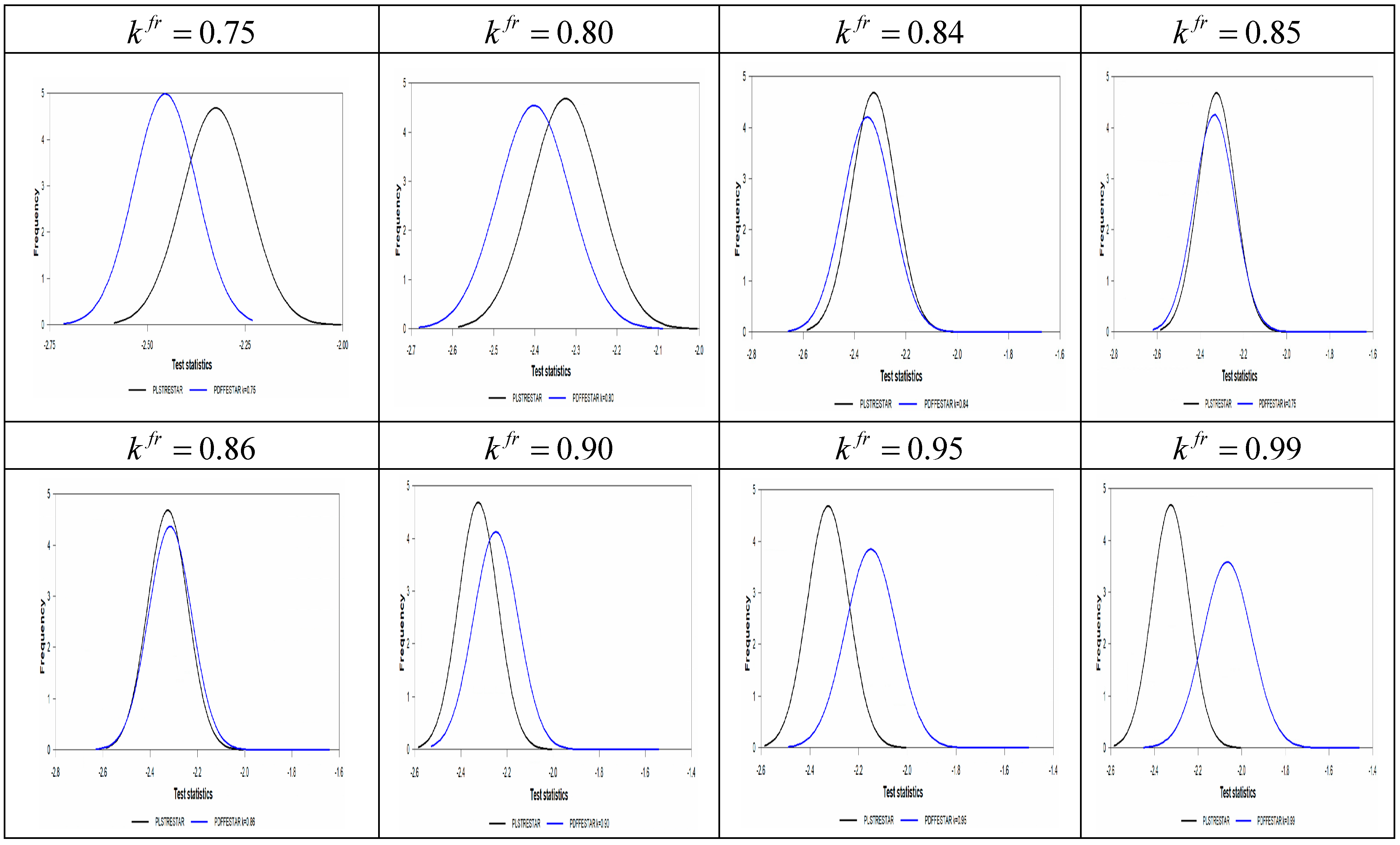
For the short T panel, the UO test with symmetrical state-dependent size nonlinearity ESTAR (1) matched with more country data than the EO test, including asymmetric state-dependent size nonlinearity AESTAR (1), and the validity of the PPP hypothesis was accepted for 5 countries with the EO test and for 12 countries with the UO test. By applying the SPS methodology, we saw how many countries in the ESTAR (1)-type state-dependent size nonlinearity panel sample are compatible with this functional structure. This good fit, provided in 12 of 34 countries, corresponds to approximately 35% of the entire sample. Distributions of empirical test results are given in the bottom row of each test in

Table 14. State-dependent nonlinear SPSM results for short T panel: 2010:1–2020:3.

	UO		EO
Switzerland	−2.285 (0.043)	Switzerland	3.539 (0.079)
Netherlands	−2.175 (0.055)	Portugal	3.098 (0.089)
Portugal	−2.145 (0.059)	New Zealand	3.004 (0.091)
Germany	−2.113 (0.064)	Malaysia	2.922 (0.098)
Spain	−2.081 (0.071)	Netherlands	2.839 (0.111)
Malaysia	−2.047 (0.077)	Germany	2.767
Italy	−2.018 (0.085)	Spain	2.696
Russia	−1.988 (0.088)	Italy	2.623
Denmark	−1.958 (0.091)	Russia	2.556
Romania	−1.934 (0.096)	Romania	2.502
Iceland	−1.909 (0.098)	France	2.445
Ireland	−1.885 (0.102)	Ireland	2.403
France	−1.862	UK	2.359
S. Korea	−1.837	Denmark	2.312
New Zealand	−1.811	Iceland	2.262
Austria	−1.784	S. Korea	2.214
Poland	−1.754	Greece	2.162
Turkey	−1.725	Australia	2.107
Belgium	−1.703	Thailand	2.051
Slovakia	−1.678	Austria	2.000
Mexico	−1.652	Poland	1.951
S. Arabia	−1.621	India	1.901
Greece	−1.593	Belgium	1.861
India	−1.567	S. Arabia	1.820
Japan	−1.540	Slovakia	1.776
Argentina	−1.507	Turkey	1.733
Hungary	−1.470	Mexico	1.681
Brazil	−1.434	Hungary	1.624
Colombia	−1.394	Japan	1.556
Canada	−1.351	Argentina	1.472
UK	−1.288	Canada	1.435
Australia	−1.206	Brazil	1.383
Thailand	−1.151	Sweden	1.382
Sweden	−1.074	Colombia	1.380
12		5

. Among these distributions, the nonlinearity of the ESTAR (1) structure explains the real exchange rate dynamics better than the nonlinearity of the AESTAR (1) type, which shows itself with the UO test results being closer to the normal distribution, while the EO test results are skewed to the left.

In Section 3, where we detailed the small sample characteristics, we explained why tests with structural breaks should be used, and the quasi-PPP and PPP hypotheses were met in the case of permanent and temporary breaks. The PPP hypothesis is valid under the fixed mean condition depending on the theoretical findings. It is well known that the quasi-PPP hypothesis may emerge if the sample data faced crises or other economic phenomena, such as rapid technology change, leading to a structural break in the real exchange rate variable.

This structural break change leads to permanent long-run mean change as well. Finally, it is also discussed in Sollis’s [14] study that a temporary break structure due to appreciation and depreciation of the real exchange rate that returns to the same fixed long-run means can provide the original PPP hypothesis. In this study, we tried to evaluate the results by model C of the logistic smooth transition trend that best captures temporary and permanent breaks. The model C structure, by its nature, can model the permanent break, while it can also model temporary break behaviors. Therefore, the model C structure will better compare the obtained results, such as original PPP, quasi-PPP (permanent break), or quasi-PPP (temporary break), which can be classified as original PPP. Therefore, the SPS method employed model C of the panel unit root test, including the structural break in their testing procedure. In

Table 15. Time-dependent and hybrid SPSM results for short T panel: 2010:1–2020:3.

	PLSTTESTAR (1)		PLSTTTAR		PLSTT
Greece	−3.837 (0.000)	Greece	8.833 (0.000)	Greece	−3.992 (0.000)
Malaysia	−3.768 (0.000)	Iceland	8.335 (0.000)	Sweden	−3.900 (0.000)
Switzerland	−3.699 (0.000)	Canada	8.094 (0.002)	Malaysia	−3.871 (0.042)
Portugal	−3.634 (0.000)	UK	7.909 (0.033)	India	−3.842 (0.072)
India	−3.586 (0.000)	Sweden	7.741 (0.087)	Russia	−3.814 (0.096)
Argentina	−3.540 (0.000)	India	7.597 (0.103)	Portugal	−3.790 (0.128)
Turkey	−3.501 (0.000)	Turkey	7.448	Canada	−3.763
Iceland	−3.464 (0.000)	Portugal	7.293	Mexico	−3.737
S. Korea	−3.431 (0.000)	Malaysia	7.144	Brazil	−3.711
Sweden	−3.400 (0.000)	S. Arabia	7.001	New Zealand	−3.684
Canada	−3.369 (0.000)	Mexico	6.858	UK	−3.655
Colombia	−3.342 (0.000)	New Zealand	6.729	S. Arabia	−3.625
S. Arabia	−3.315 (0.000)	Hungary	6.621	Turkey	−3.595
Russia	−3.287 (0.000)	Slovakia	6.510	Hungary	−3.564
Spain	−3.261 (0.002)	Russia	6.406	Slovakia	−3.531
Slovakia	−3.236 (0.018)	Spain	6.308	Spain	−3.500
Thailand	−3.213 (0.026)	Poland	6.208	Thailand	−3.468
Belgium	−3.188 (0.039)	Thailand	6.107	Netherlands	−3.433
UK	−3.160 (0.045)	Argentina	5.994	Poland	−3.394
New Zealand	−3.132 (0.057)	Netherlands	5.900	S. Korea	−3.359
Austria	−3.099 (0.068)	Brazil	5.809	Argentina	−3.324
Mexico	−3.062 (0.085)	Ireland	5.705	Ireland	−3.294
Italy	−3.024 (0.095)	S. Korea	5.584	Australia	−3.264
Hungary	−2.993 (0.121)	Belgium	5.498	Japan	−3.233
Australia	−2.960	Italy	5.430	Italy	−3.205
Poland	−2.932	Denmark	5.361	Switzerland	−3.178
Brazil	−2.897	Australia	5.278	Austria	−3.144
Ireland	−2.854	Austria	5.183	Denmark	−3.103
Denmark	−2.800	Switzerland	5.100	Colombia	−3.057
Germany	−2.758	Japan	5.002	Romania	−3.001
Japan	−2.705	Romania	4.878	Germany	−2.930
Netherlands	−2.671	Germany	4.732	Belgium	−2.827
Romania	−2.608	Colombia	4.558	France	−2.629
France	−2.560	France	4.178	Iceland	−2.477
	23		5		5

, SPSM results of the tests based on model C, including the structural break, are given as mentioned above. The full sample results show that the PLSTTESTAR and PLSTTTAR models are significant at 1%, and the PLSTT unit root test is significant at the 5% level. However, when the SPS methodology is applied, the number of stationary and nonstationary countries shows that the PLSTTESTAR test fits the data much better than the other two tests.

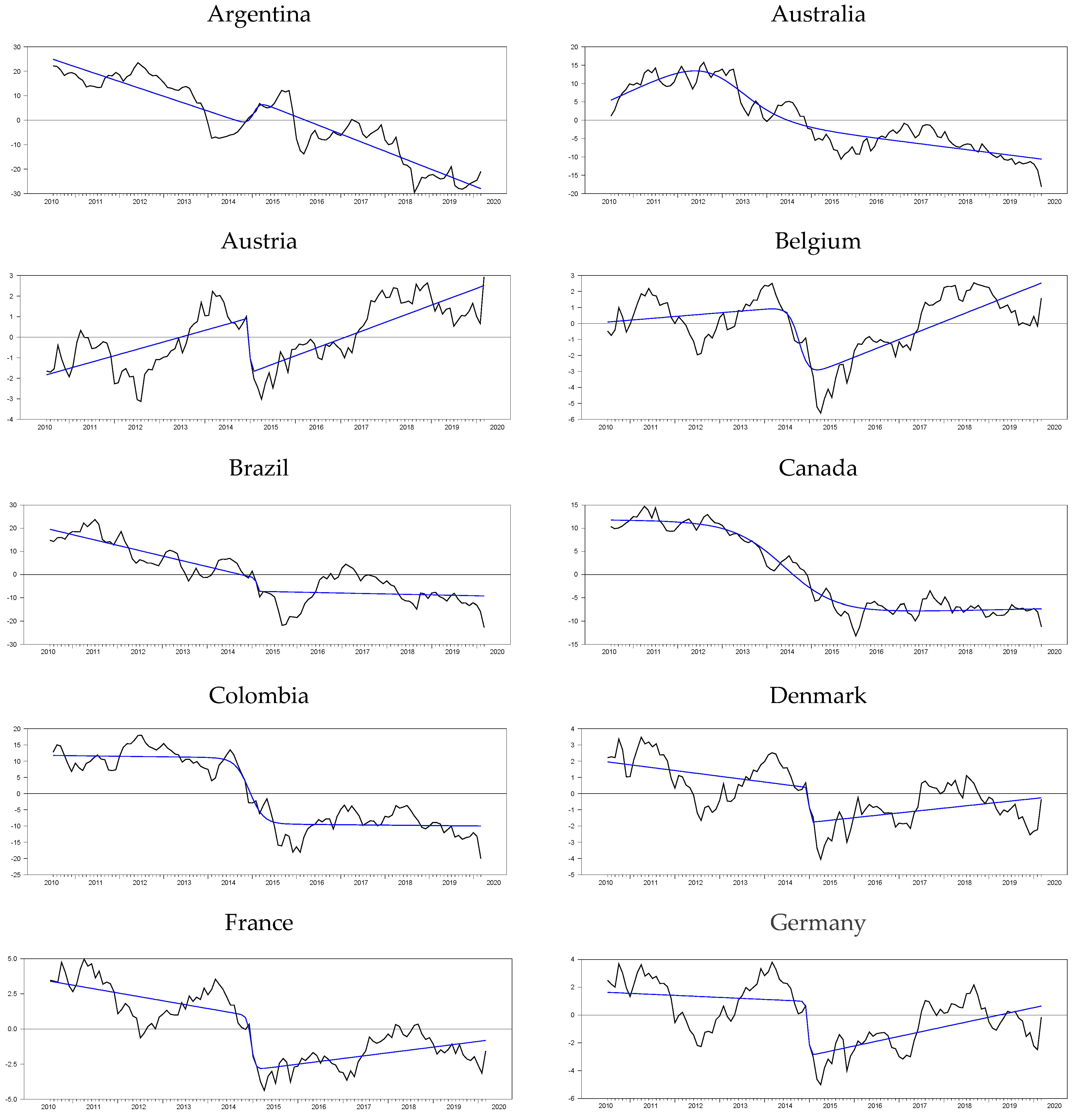
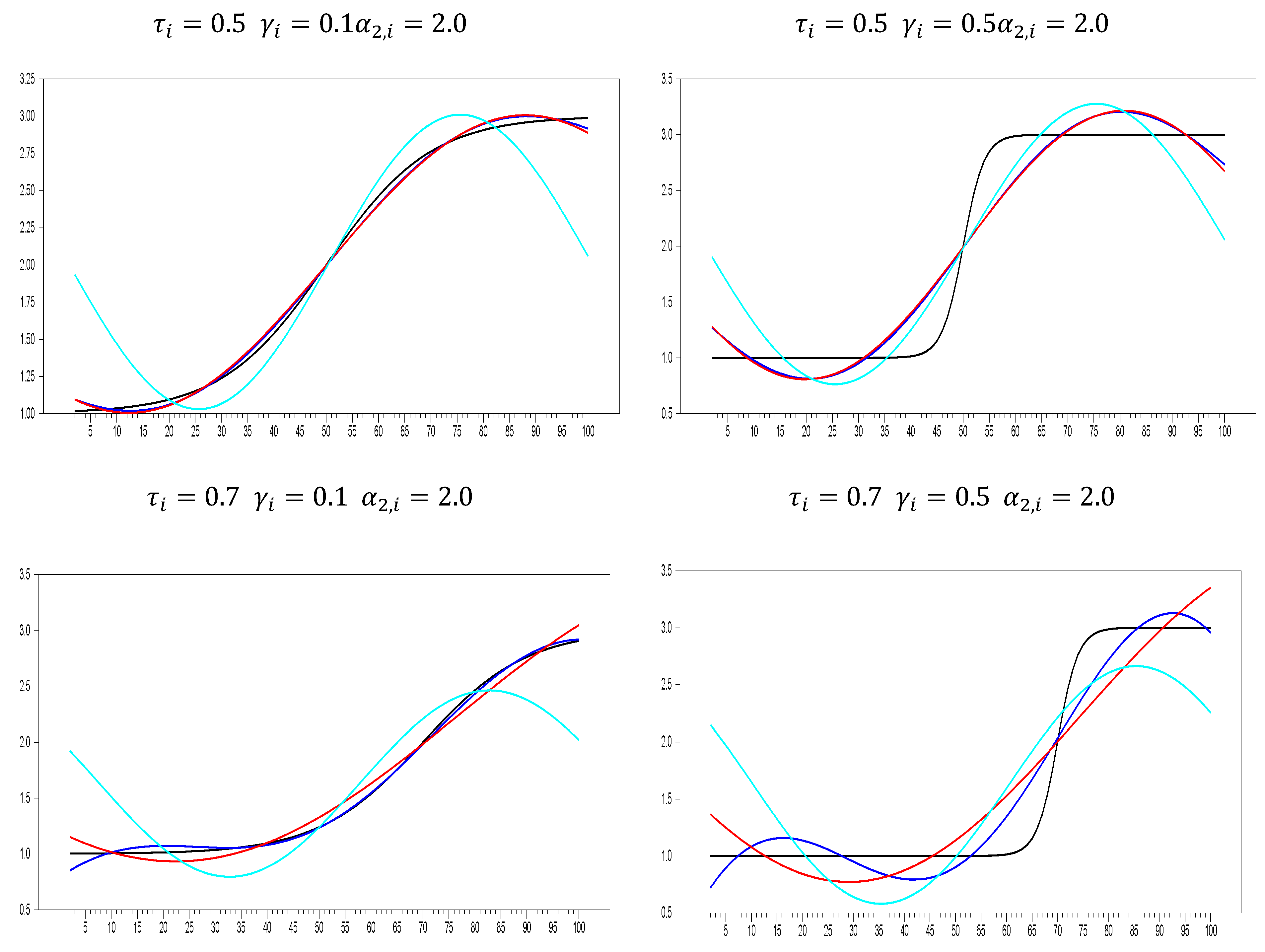
Although it is also seen that the logistic smooth transition model C structure better captures the features of the real exchange rate data as represented graphically in Figure 2, this good fit is not general enough to cover all countries. In addition, it is seen that TAR-type nonlinearity is very insufficient to explain the real exchange rate dynamics compared with ESTAR (1) nonlinearity. While the PLSTTESTAR test found 23 stationary countries, five-country stationary is found in the PLSTTTAR unit root test. These countries are almost identical to those in the PLSTT test (Greece, Canada, Sweden, and the UK). Here, TAR nonlinearity had a significant effect only on Iceland, and while it was the worst significant in the PLSTT test, it ranked the second-best significant test result in the PLSTTTAR test. Therefore, it is seen that the TAR structure is only a good fit for the Icelandic real exchange rate data. If we compare the SPSM results of the UO and EO tests with the PLSTTESTAR test, the situation does not change much; it is understood that the model or functional structures that provide the best compatibility with the real exchange rate series are in the PLSTTESTAR unit root test. PLSTTESTAR explains about 67% of the full sample, while its closest follower, the UO test, explains 35%. In order to better interpret these results, it is useful to make nonlinear parameter estimations of the sample at hand. If we show its consistency with the results in the section where we discussed the power analysis, it will be evident that the unit root test we propose fits better with the real exchange rate dynamics than the current linear or nonlinear panel unit root tests. For this purpose, the break parameters obtained from the structural break tests will be evaluated according to the results we obtained in the power analysis. Later, whether the PLSTTESTAR test in power analysis is close to the estimated parameters in the high-power regions will be discussed. Depending on the two-stage test procedure, in the second stage, after removing the nonlinear trend, how well the real exchange series fit the ESTAR (1)-type structure will be investigated by making nonlinear parameter estimations.

In the power analysis section, we saw that different parameters of the logistic smooth transition trend increase the power of the proposed test. A break size of 5 units is used for the moderate break and 10 for the higher break in the power analysis. When we look at the country-by-country estimates here, the value of the break parameter is very high in almost all countries as shown in

Table 16. Logistic smooth transition (model C) parameter estimates.

	${\widehat{\mathit{\alpha }}}_{1,\mathit{i}}$	${\widehat{\mathit{\alpha }}}_{2,\mathit{i}}$	${\widehat{\mathit{\beta }}}_{1,\mathit{i}}$	${\widehat{\mathit{\beta }}}_{2,\mathit{i}}$	${\mathit{\gamma }}_{\mathit{i}}$	${\mathit{\tau }}_{\mathit{i}}$	$\left|{\widehat{\mathit{\alpha }}}_{2,\mathit{i}}-{\widehat{\mathit{\alpha }}}_{1,\mathit{i}}\right|$	Difference
Arg.	25.354	15.463	−0.503	−0.085	1.256	0.473	9.891	52.801
Aust.	4.995	−0.689	0.468	−0.596	0.169	0.280	5.684	16.044
Austria *	−1.883	−3.599	0.051	0.017	13.027	0.469	1.716	−4.338
Belgium *	0.069	−8.397	0.019	0.074	0.734	0.447	8.465	−2.436
Brazil	19.895	−25.261	−0.383	0.350	12.882	0.479	45.156	28.733
Canada	11.789	−21.080	−0.008	0.025	0.144	0.410	32.870	19.088
Col.	11.764	−20.521	−0.014	0.003	0.523	0.463	32.285	21.742
Den *	1.985	−5.113	−0.030	0.054	13.143	0.470	7.099	2.215
France	3.442	−8.202	−0.046	0.080	1.981	0.466	11.644	4.211
Germany	1.648	−7.716	−0.012	0.070	3.711	0.467	9.364	0.988
Greece	8.146	−11.245	−0.132	0.125	1.036	0.456	19.391	12.028
Hungary	7.633	−11.394	−0.117	0.122	0.476	0.420	19.027	10.708
Iceland	−26.267	220.933	−1.261	−0.193	0.044	0.517	247.200	−21.400
India *	6.875	−7.017	−0.417	0.451	0.274	0.423	13.892	2.598
Ireland	6.499	−9.785	−0.071	0.065	1.060	0.458	16.284	10.404
Italy	1.872	−4.371	0.012	−0.004	0.814	0.454	6.242	3.428
Japan	27.417	−27.159	−0.701	0.638	0.539	0.554	54.576	33.806
Malaysia	7.326	−18.016	−0.056	0.108	1.212	0.521	25.342	11.799
Mexico	7.454	−30.928	0.056	0.092	0.256	0.529	38.381	13.588
Neth *	−0.249	−5.903	0.036	0.028	1.428	0.463	5.654	−1.601
New Z *	−5.170	9.684	0.272	−0.348	0.533	0.465	14.854	−0.543
Poland	5.161	−16.725	−0.077	0.172	0.391	0.527	21.885	5.483
Portugal	1.712	−2.417	−0.019	0.017	1.021	0.422	4.129	2.646
Rom *	1.778	−9.199	0.007	0.050	0.258	0.535	10.977	2.477
Russia	11.825	−34.130	0.030	0.116	1.551	0.445	45.956	17.108
S. Arabia	−10.665	26.363	0.124	−0.230	0.334	0.481	37.028	−13.787
S. Korea	−7.790	13.155	0.019	−0.040	0.245	0.340	20.945	−10.692
Slovakia *	0.077	−6.037	0.045	0.011	0.524	0.464	6.115	−0.503
Spain *	2.118	−7.657	−0.006	0.051	1.294	0.461	9.775	2.336
Sweden	6.208	2.826	0.091	−0.266	0.404	0.390	3.383	17.755
Swit *	1.000	10.128	−0.060	−0.063	13.267	0.466	9.127	4.201
Thailand	−4.681	−22.362	0.098	0.222	0.548	0.543	17.680	−14.882
Turkey	15.924	18.955	−0.232	−0.272	1.141	0.437	3.031	39.741
UK *	−6.127	−5.752	0.260	−0.183	0.598	0.604	0.376	−2.921
Total					76.817	15.799	815.423
Average					2.259	0.465	23.983

Note: (*) indicates the countries having temporary breaks.

.

The average of 34 countries for the break parameter was 23.983. The result obtained in Table 16 signifies to a high break parameter vlue. With this break parameter, it is evident that the tests without a structural break, especially the IPS test, have very little power against this data structure. As a matter of fact, as a result of the test, the bootstrap IPS test could not provide stationarity either in the intercept or in the intercept and trend models. The second parameter we will examine is the transition rate parameter. As the transition speed parameter decreases, the power of the tests with logistic smooth transition increases. The first thing to note here is that the larger the break parameter, the higher the value of the gamma parameter, which adjusts the smoothness of this transition speed. For break magnitude values of 5 and 10, 5 transition slopes correspond to a relatively high transition speed, while in the case of a higher break size such as 24, 5 transition slopes correspond to a relatively low value. In this sense, 2.259 average transition speeds indicate a smooth transition according to the size of the break.

For this reason, the power of the PLSTTESTAR test and the other tests, including logistic smooth transition, is increasing. Finally, we observed that the threshold value being relatively in the middle of the sample increases the power of the tests containing the logistic smooth transition trend. Therefore, we see that almost all countries experience a break around 0.5, that is, at the midpoint of the sample. As for the threshold location, the country with the break structure at the beginning of the sample is Australia, at 0.280 points of the sample, while the latest break day belongs to UK data with 0.604. The average of the 34 countries was found to be 0.465. The break size is 23.983, the transition rate is 2.259, and the threshold value is 0.465. According to these results, the power of the tests, including logistic smooth transition, will be high. If we look at the empirical test results, the tests, including logistic smooth transition, have rejected the null hypothesis more significantly than any other test structure. The most significant of these tests is the model C structure, in which they reject the null hypothesis. PLSTT, PLSTTAR, and PLSTESTAR tests rejected the null hypothesis at 0.021, 0.000, and 0.000 significance levels. Likewise, while the state-dependent unit root tests UO and EO rejected the null hypothesis at 0.047 and 0.063 significance levels, the IPS test could not reject the PPP hypothesis with 0.299. These results show us that logistic smooth transition alone can capture the dynamics of the PPP hypothesis or real exchange data. In addition, when we compare the tests that include structural breaks with those that do not, it is understood that the tests containing breaks yield results in line with the above-mentioned power analysis and reject the null hypothesis at a higher significance level. The EO and UO tests are asymmetrical and symmetrical versions of the ESTAR (1) structure. When the test results are examined, it is seen that the EO test can reject the null hypothesis at a 0.063 significance level, while the UO test provides a better fit with the data with a 0.047 significance level. The explanation for this situation shows that the behavior of the real exchange rate variable is more suitable for the symmetrical ESTAR (1) structure and the power of the EO test is lower than the UO test, which has the ESTAR (1) structure in the symmetrical structure since unnecessary parameter estimation is made. The rejection of the null hypothesis by the UO test indicates that some countries in the panel sample can be modeled with the ESTAR (1) structure, and thus, the PPP hypothesis can be confirmed for these countries.

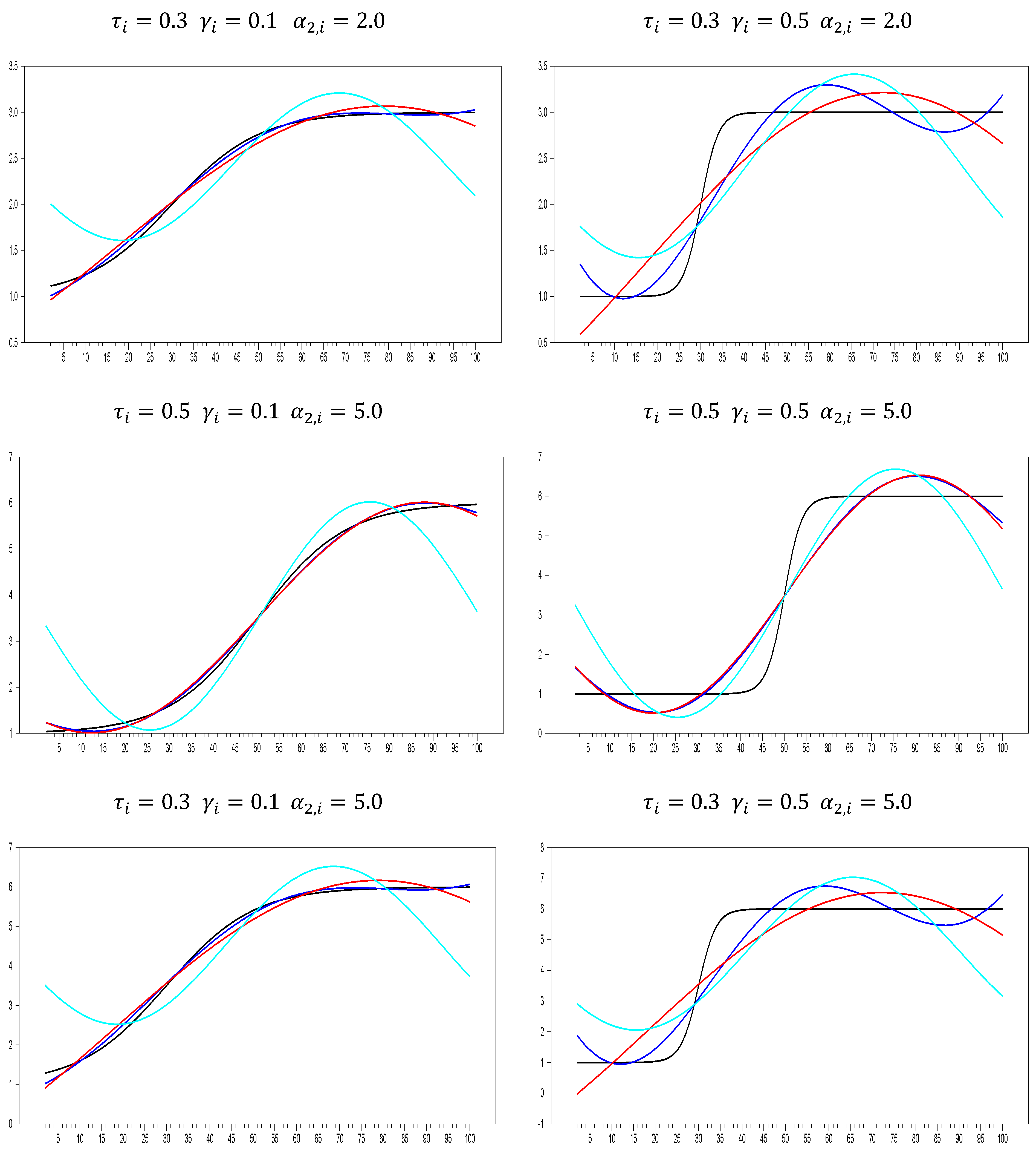
The fact that six countries are stationary in the PLSTTTAR model C with SPS methodology shows that nonlinearity in TAR type does not comply with exchange rate dynamics. In addition, the UO test, which includes the ESTAR (1) model, showed that 12 countries have stationary in SPSM analysis and better adapt to exchange rate dynamics. For this reason, it is useful to investigate how much ESTAR (1)-type nonlinear structure remains in the remaining part after the logistic smooth transition de-trend series is estimated. Accordingly, estimations were performed as suggested in the article [19] and discussed in the power analysis of the ESTAR (1) structure. The results obtained in

Table 17. ESTAR parameter estimates.

Countries	${\mathit{\delta }}_{\mathit{i}}$	$\mathit{t}-\mathit{s}\mathit{t}\mathit{a}\mathit{t}$  $\mathbf{for} {\mathit{\delta }}_{\mathit{i}}$
Argentina	7.51 × 10−4	2.831
Australia	0.004	3.340
Austria	0.037	2.453
Belgium	0.018	2.907
Brazil	3.81 × 10−4	2.372
Canada	0.007	2.489
Colombia	0.003	3.567
Denmark	0.019	3.155
France	0.023	3.032
Germany	0.011	2.258
Greece	0.062	5.142
Hungary	0.002	1.725
Iceland	6.34 × 10−4	1.799
India	0.008	4.086
Ireland	0.012	3.083
Italy	0.030	3.338
Japan	6.78 × 10−4	2.073
Malaysia	0.017	5.604
Mexico	0.003	2.875
Netherlands	0.012	2.423
New Zealand	0.003	3.273
Poland	0.003	1.966
Portugal	0.077	4.396
Romania	0.002	2.094
Russia	7.07 × 10−4	2.411
S. Arabia	0.007	3.421
S. Korea	0.006	3.832
Slovakia	0.095	3.773
Spain	0.023	3.106
Sweden	0.008	3.077
Switzerland	0.001	2.431
Thailand	0.002	1.507
Turkey	7.55 × 10−4	2.000
UK	0.005	3.089
Average	1.48 × 10−2

support the power analysis.

The transition rate parameter ${\delta }_i$ estimate average is 0.01 for 34 countries. This situation corresponds to the area of high power of the proposed test. In addition, the low transition speed rate in nonlinearity in the state-dependent structure increases the power of the tests with ESTAR (1) nonlinearity. The graphs of the ESTAR (1) estimations given in Figure 3 strikingly demonstrate this low transition speed (slope) rate. As discussed in Kapetanios et al. [19], it has been shown that for low transition speed rates, the power is low for Enders and Granger [54] (EG) tests, which deal with TAR-type nonlinearity, and the ADF test, which has a linear structure. In the analysis here, the linear ADF test corresponds to the PLSTT test, while the EG test corresponds to the PLSTTAR test. In line with the nonlinear model estimates obtained in Table 16 and Table 17, it can be easily understood that both the PLSTT test and the PLSTTAR test face data with a low power structure, with their testing procedure including linear and TAR-type nonlinearity for the stochastic process. SPSM test results also confirm this result.

With the sequential panel selection method (SPSM), although the null hypothesis was rejected at the border, the number of countries rejecting this hypothesis can be determined. Thus, it can be concluded that other methodologies should be proposed to enable more realistic testing of the PPP hypothesis. How many countries contributed to rejecting the null hypothesis in a panel data sample that concludes that the model under consideration increases the power of explaining economic events that much? In this sense, whether or not the newly proposed test has undertaken this task, it has tried to examine it using SPSM methodology. It is evident from the test results (Table 13, Table 14, Table 15, Table 16 and Table 17) that the functional structures of both the logistics smooth transition trend and the exponential smooth transition type play an active role in the real exchange rate dynamics. However, more importantly, the PLSTTESTAR test, which includes both functional structures at a significance level of less than 1%, leads to the acceptance of the PPP hypothesis that supports the proposed test. We cannot see the same success from its closest competitor, the PLSTTTAR model. When the SPSM comparison of these two tests is made, it is understood that the PLSTTTAR test is high due to the individual test results obtained in Greece, Iceland, and Canada, which are 27,084, 15,699, and 14,776, respectively.

On the other hand, when we return back to the Table 16, it is indeed serving empiriacal distribution which is a left-skewed so that many test values are small. The last two rows of Table 16 show the distribution of empirical test results for PLSTTESTAR and PLST tests. Since these two tests are t-tests, higher test values are seen as values that go to the left of the distribution. PLST empirical test results are also relatively right-skewed and have extreme values. The empirical test value distribution of the PLSTTESTAR test is nearly normally distributed and has no extreme value. This empirical test value distribution shows that the PLSTTESTAR test homogeneously obtains empirical test value results close to high values, thus conducive to the stationarity of many more countries in the SPSM methodology. The UO test is relatively high in all countries, with a balance similar to the empirical test result distribution in the PLSTTESTAR test, and provided the PPP hypothesis in 12 countries, while the PLSTT model provided the PPP hypothesis in only 6 countries. While the PLSTT and UO tests separately provided the PPP hypothesis in 6 and 12 countries, the PLSTTESTAR test, which was used together, provided the PPP hypothesis in 23 countries. This case shows us that the functional structures proposed in the PLSTTESTAR test in the short T panel better adapt to the real exchange rate dynamics. In order to better illustrate this situation, the ESTAR (1) model estimates and nonlinear parameter estimates of the PLSTT model are discussed in [18]. In the section where we explained the small sample characteristics, we explained why tests with structural breaks should be used, and the quasi-PPP and PPP hypotheses were met in the case of permanent and temporary breaks. We mentioned this issue at the beginning of the empirical part.

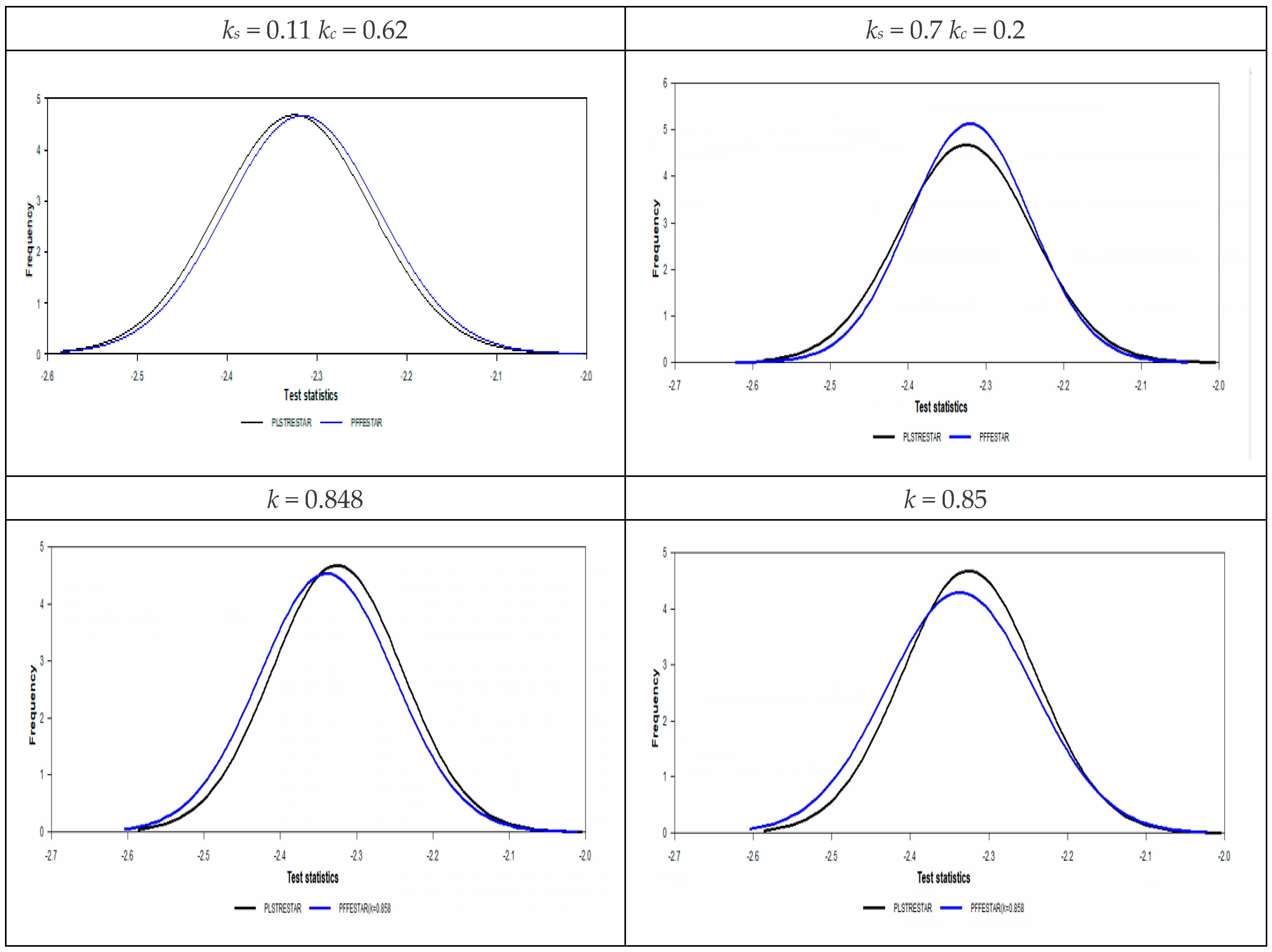
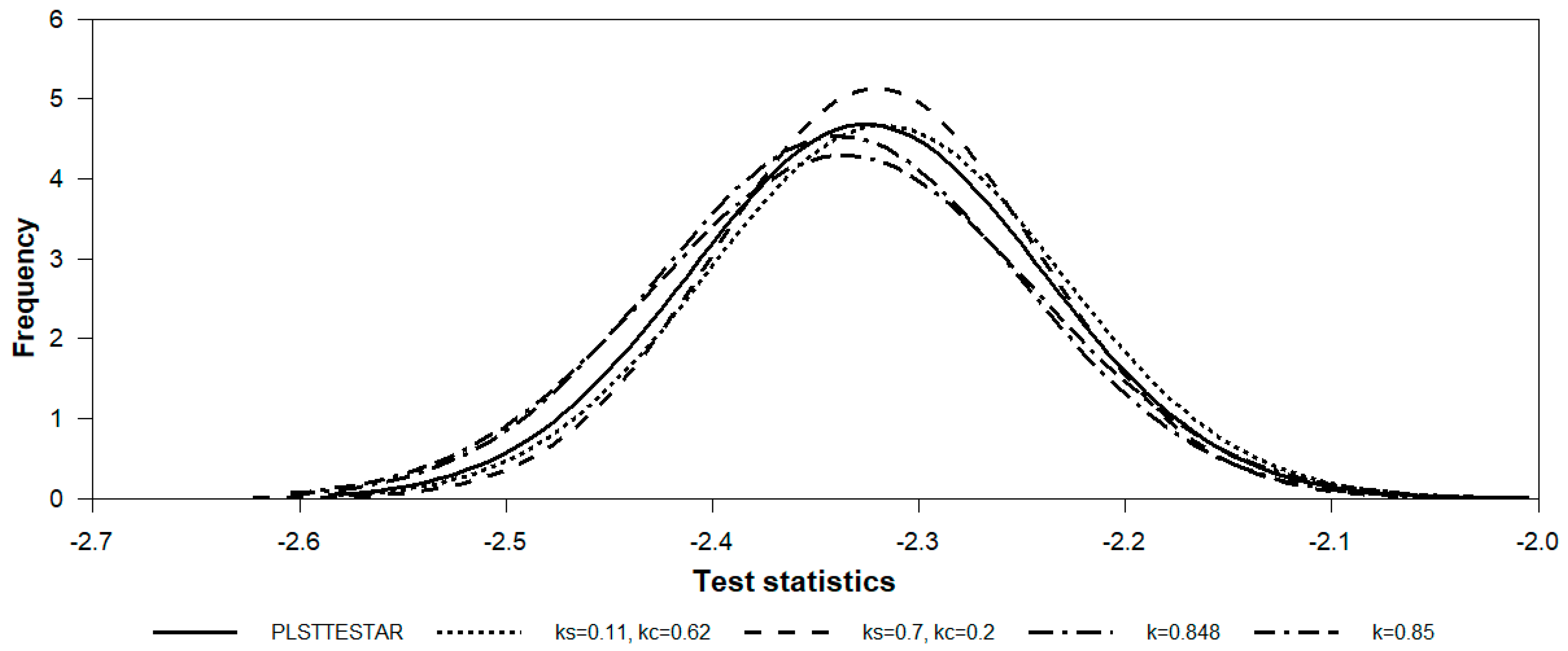
In order to better understand this issue, we add a column named as“difference” in Table 16. Estimates in this column are obtained by subtracting the start and endpoints of the nonlinear trends for the logistic smooth transition model C. As this difference value grows, it is understood that the nonlinear trend catches a permanent break, and as it becomes smaller, a temporary break occurs. Moreover, examples of the temporary break structure can be seen in Figure 3. Belgium, India, Slovakia, and the UK are a good example of this temporary break situation. If we look at the logistics and smooth transition trends of these countries, they all have a temporary break structure in such a way that the starting and ending points are close to each other and form a U shape. To illustrate this better, we compute the differences of the logistic smooth transition start and endpoints from the last column of Table 16, which are −2.436, 2.598, −0.503, and −2.921 for Belgium, India, Slovakia, and the UK, respectively. While these countries exhibit a temporary break structure, Canada and Colombia are good examples of the permanent break, with difference values of 28,733 and 19,088, respectively. Although countries such as Belgium, India, Slovakia, and the UK are stationary with the PLSTTESTAR (1) model, it can be concluded that the original PPP hypothesis is met within the temporary break structure proposed in the article. The results obtained based on these distinctions are summarized in

Table 18. Summary of SPSM results for short T panel: 2010:1–2020:3.

	PLSTESTAR	ESTAR	AESTAR	PLSTTAR	PLSTT
Argentina	+					Quasi-PPP
Australia						Not
Austria	+					Quasi-PPP
Belgium *	+					Quasi-PPP *
Brazil						Not
Canada	+			+		Quasi-PPP
Colombia	+					Quasi-PPP
Denmark		+				PPP
France						Not
Germany		+				PPP
Greece	+			+	+	Quasi-PPP
Hungary						Not
Iceland	+	+		+		Quasi-PPP
India *	+			+	+	Quasi-PPP *
Ireland		+				PPP
Italy	+	+				PPP
Japan						Not
Malaysia	+	+	+		+	PPP
Mexico	+					Quasi-PPP
Netherlands		+	+			PPP
New Zealand	+		+			PPP
Poland						Not
Portugal	+	+	+		+	PPP
Romania		+				PPP
Russia	+	+			+	PPP
S. Arabia	+					Quasi-PPP
S. Korea	+					Quasi-PPP
Slovakia *	+					Quasi-PPP *
Spain	+	+				PPP
Sweden	+			+	+	Quasi-PPP
Switzerland	+	+	+			PPP
Thailand	+					Quasi-PPP
Turkey	+					Quasi-PPP
UK *	+			+		Quasi-PPP *

Note: (+) indicates the convenient models for each country and (*) implies that Belgium, India, Slovakia, and the UK are stationary with the PLSTTESTAR (1) model with having temporary break.

.

We repeated the short T panel analysis in the long T panel, provided as Appendix A. The results for this period covering the years 1994:1–2020:3 are the same as those obtained for the short T panel. In the long term, the significance levels of all tests increased, and even in the linear model, the sieve-bootstrap IPS test resulted in the acceptance of the PPP hypothesis in 11 countries. If we look at the summary tables, PLSTTESTAR accepted the PPP hypothesis in 31 of 34 countries, while its closest follower, the UO test, remained in 25 countries. In terms of ranking, the status of the other tests remained the same as in the short panel T. The EO test results increased from 5 to 25 stationary countries, while the PLSTT test result went from 6 to 17 stationary countries, and the PLSTTTAR test results from 6 to 17 countries. Estimations for the nonlinear parameters of the logistic smooth transition gave results similar to those of the short T panel. The mean break size was found to be 15,152 for 34 countries, the mean of the transition speed parameter was 0.688, and the mean of the threshold was 0.443. This parameter combination belongs to a more powerful PLSTTESTAR test region; hence, the acceptance rate increased from 23 countries to 31 countries. All the comments we made in the short T panel are valid in the long T panel. The transition speed of the ESTAR (1) function is also almost the same as the 0.01 value we found for the short T panel. It is evident that the PLSTTESTAR test reflects the real exchange rate dynamics better than other tests. In the long T panel, the temporary break search is performed over the difference value. The results are indicated as quasi-PPP* in the Table 18. The results obtained from the long T panel show that the unit root test in the PLSTTESTAR structure we recommend best captures the real exchange rate dynamics, regardless of whether they are short (local) or long term. Therefore, we have clearly shown that the quasi-PPP* hypothesis and the logistic smooth transition trend structure can be used in theoretical and empirical studies for the real exchange rate dynamics. In addition to the ESTAR (1) structure, this logistic smooth transition model C structure has been identified as a significant complementary functional structure for testing the validity of PPP hypothesis.

6. Concluding Remarks

This study examines the validity of the PPP proposition for 34 European and selected global countries. For this purpose, we propose a new unit root test for cross-sectionally dependent heterogeneous panels that allows for both gradual structural breaks and symmetric nonlinear adjustment toward the equilibrium level.

The alternative hypothesis stationary is obtained by symmetric adjustment due to exponential smooth transition autoregression (ESTAR) around a nonlinear trend. This alternative hypothesis characterized the main features of the REER data. Moreover, we provided small sample properties for the newly proposed test. Therefore, the newly proposed tests fulfill the gaps in obtaining wrong conclusions due to the mismodeling of the REER series. Furthermore, cross-section dependency is another primary source of misspecifications in testing the PPP hypothesis. Open economies are faced with spillover effects, common shocks, and other sources of cross-section dependency. Therefore, by introducing a common correlated estimation and bootstrap algorithm for this highly nonlinear structure, we also gave solutions for these misspecifications in testing the PPP hypothesis. For further research, the researcher may employ our newly proposed test for different countries and sample periods for the REER series or other financial variables. Lastly and more importantly, we gave the approximate limiting distribution of the newly proposed test for the first time in the literature.

References

1. Rogoff, K. The purchasing power parity puzzle. J. Econ. Lit. 1996, 34, 647–668. [Google Scholar]
2. Taylor, M.P.; Sarno, L. The Behavior of Real Exchange Rates during the Post-Bretton Woods Period. J. Int. Econ. 1998, 46, 281–312. [Google Scholar] [CrossRef]
3. Corbae, D.; Ouliaris, S. Cointegration and tests of purchasing power parity. Rev. Econ. Stat. 1988, 70, 508–511. [Google Scholar] [CrossRef]
4. Fisher, E.O.N.; Park, J.Y. Testing purchasing power parity under the null hypothesis of co-integration. Econ. J. 1991, 101, 1476–1484. [Google Scholar] [CrossRef]
5. Froot, K.A.; Rogoff, K. Perspectives on PPP and long-run real exchange rates. Handb. Int. Econ. 1995, 3, 1647–1688. [Google Scholar]
6. Dumas, B. Dynamic equilibrium and the real exchange rate in a spatially separated world. Rev. Fin. Stud. 1992, 5, 153–180. [Google Scholar] [CrossRef]
7. Sercu, P.; Uppal, R.; Van Hulle, C. The exchange rate in the presence of transaction costs: Implications for tests of purchasing power parity. J. Financ. 1995, 50, 1309–1319. [Google Scholar] [CrossRef]
8. Michael, P.; Nobay, A.R.; Peel, D.A. Transactions costs and nonlinear adjustment in real exchange rates; An empirical investigation. J. Polit. Econ. 1997, 105, 862–879. [Google Scholar] [CrossRef]
9. Taylor, A.M.; Taylor, M.P. The purchasing power parity debate. J. Econ. Perspect. 2004, 18, 135–158. [Google Scholar] [CrossRef] [Green Version]
10. Hegwood, N.D.; Papell, D.H. Quasi purchasing power parity. Int. J. Fin. Econ. 1998, 3, 279–289. [Google Scholar] [CrossRef]
11. Perron, P. The great crash, the oil price shock, and the unit root hypothesis. Econometrica 1989, 57, 1361–1401. [Google Scholar] [CrossRef] [Green Version]
12. Papell, D.H.; Prodan, A. Additional Evidence of Long-Run Purchasing Power Parity with Restricted Structural Change. J. Money Credit Bank. 2006, 38, 1229–1349. [Google Scholar] [CrossRef]
13. Lundbergh, S.; Teräsvirta, T.; Van Dijk, D. Time-varying smooth transition autoregressive models. J. Bus. Econ. Stat. 2003, 21, 104–121. [Google Scholar] [CrossRef]
14. Sollis, R.; Leybourne, S.; Newbold, P. Tests for Symmetric and Asymmetric Nonlinear Mean Reversion in Real Exchange Rates. J. Money Credit Bank. 2002, 34, 686–700. [Google Scholar] [CrossRef] [Green Version]
15. Christopoulos, D.K.; Leon-Ledesma, M.A. Smooth breaks and non-linear mean reversion: Post-Bretton Woods real exchange rates. J. Int. Money Fin. 2010, 29, 1076–1093. [Google Scholar] [CrossRef] [Green Version]
16. Koop, G.; Potter, S. A flexible approach to parametric inference in nonlinear and time varying time series models. J. Econ. 2010, 159, 134–150. [Google Scholar] [CrossRef] [Green Version]
17. Omay, T.; Hasanov, M.; Emirmahmutoğlu, F. Structural Break, Nonlinearity, and Asymmetry: A re-examination of PPP proposition. Appl. Econ. 2017, 50, 1289–1308. [Google Scholar] [CrossRef] [Green Version]
18. Leybourne, S.; Newbold, P.; Vougas, D. Unit roots and smooth transitions. J. Time Ser. Anal. 1998, 19, 83–89. [Google Scholar] [CrossRef]
19. Kapetanios, G.; Shin, Y.; Snell, A. Testing for a unit root in the nonlinear STAR framework. J. Econ. 2003, 112, 359–379. [Google Scholar] [CrossRef]
20. Omay, T.; Yildirim, D. Nonlinearity and smooth breaks in unit root testing. Econ. Lett. 2014, 1, 1–9. [Google Scholar]
21. O’Connell, P.G. The overvaluation of purchasing power parity. J. Int. Econ. 1998, 44, 1–19. [Google Scholar] [CrossRef]
22. Banerjee, A.; Marcellino, M.; Osbat, C. Some Cautions on the Use of Panel Methods for Integrated Series of Macro-Economic Data. Econ. J. 2004, 7, 322–340. [Google Scholar] [CrossRef]
23. Moon, R.; Perron, B. Testing for a unit root in panels with dynamic factors. J. Econom. 2004, 122, 81–126. [Google Scholar] [CrossRef] [Green Version]
24. Bai, J.; Serena, N.G. A PANIC Attack on Unit Roots and Cointegration. Econometrica 2004, 72, 1127–1177. [Google Scholar] [CrossRef] [Green Version]
25. Pesaran, M.H. A simple panel unit root test in the presence of cross-section dependence. J. Appl. Econ. 2007, 22, 265–312. [Google Scholar] [CrossRef] [Green Version]
26. Pesaran, M.H.; Vanessa Smith, L.; Yamagata, T. Panel unit root tests in the presence of a multifactor error structure. J. Econom. 2013, 175, 94–115. [Google Scholar] [CrossRef] [Green Version]
27. Maddala, G.S.; Wu, S. A comparative study of unit root tests with panel data and a new simple test. Oxf. Bull. Econ. Stat. 1999, 61, 631–652. [Google Scholar] [CrossRef]
28. Chang, Y. Bootstrap Unit Root Tests in Panels with Cross-Sectional Dependency. J. Econom. 2004, 120, 263–293. [Google Scholar] [CrossRef] [Green Version]
29. Smith, L.V.; Leybourne, S.; Kim, T.-H.; Newbold, P. More powerful panel data unit root tests with an application to mean reversion in real exchange rates. J. Appl. Econ. 2004, 19, 147–170. [Google Scholar] [CrossRef]
30. Cerrato, M.; Sarantis, N. Does purchasing power parity hold in emerging markets? Evidence from a panel of black market exchange rates. Int. J. Fin. Econ. 2007, 12, 427–444. [Google Scholar] [CrossRef]
31. Ucar, N.; Omay, T. Testing for unit root in nonlinear heterogeneous panels. Econ. Lett. 2009, 104, 5–8. [Google Scholar] [CrossRef]
32. Palm, F.C.; Smeekes, S.; Urbain, J.-P. Cross-sectional dependence robust block bootstrap panel unit root tests. J. Econom. 2011, 163, 85–104. [Google Scholar] [CrossRef] [Green Version]
33. Omay, T.; Hasanov, M.; Shin, Y. Testing for Unit Roots in Dynamic Panels with Smooth Breaks and Cross-sectionally Dependent Errors. Comp. Econ. 2018, 52, 167–193. [Google Scholar] [CrossRef]
34. Emirmahmutoğlu, F.; Omay, T. Reexamining the PPP hypothesis: A nonlinear asymmetric heterogeneous panel unit root test. Econ. Model. 2014, 40, 184–190. [Google Scholar] [CrossRef]
35. Çorakcı, A.; Emirmahmutoğlu, F.; Omay, T. Re-examining the real interest rate parity hypothesis (RIPH) using panel unit root tests with asymmetry and cross-section dependence. Empirica 2017, 44, 91–120. [Google Scholar] [CrossRef]
36. Omay, T.; Çorakcı, A.; Emirmahmutoğlu, F. Real interest rates: Nonlinearity and structural breaks. Emp. Econ. 2017, 52, 283–307. [Google Scholar] [CrossRef]
37. Schmidt, P.; Phillips, P.C. LM tests for a unit root in the presence of deterministic trends. Oxf. Bull. Econ. Stat. 1992, 54, 257–287. [Google Scholar] [CrossRef]
38. Sandberg, R. Testing for unit roots in nonlinear heterogeneous panels with smoothly changing trends: An application to Scandinavian unemployment rates. Emp. Econ. 2016, 51, 1053–1083. [Google Scholar] [CrossRef]
39. Im, K.S.; Pesaran, M.H.; Shin, Y. Testing for unit roots in heterogeneous panels. J. Econom. 2003, 115, 53–74. [Google Scholar] [CrossRef]
40. Fuartes, A.; Smith, R. Panel Time Series. 2012. Available online: https://www.researchgate.net/publication/277293522 (accessed on 25 February 2023).
41. Omay, T.; Kan, Ö.E. Re-examining the threshold effects in the inflation-growth nexus with cross-sectionally dependent non-linear panel: Evidence from six industrialized economies. Econ. Model. 2010, 27, 996–1005. [Google Scholar] [CrossRef]
42. Pesaran, M.H. General diagnostic tests for cross-section dependence in panels. In Cambridge Working Papers in Economics 0435; Faculty of Economics, University of Cambridge: Cambridge, UK, 2004. [Google Scholar]
43. Pesaran, M.H. Estimation and Inference in Large Heterogeneous Panels with a Multifactor Error Structure. Econometrica 2006, 74, 967–1012. [Google Scholar] [CrossRef] [Green Version]
44. Edison, H.; Kloveland, J. A quantitative reassessment of the PPP hypothesis. J. Appl. Econ. 1987, 2, 309–333. [Google Scholar] [CrossRef] [Green Version]
45. Bai, J.; Carrion-I-Silvestre, J.L. Structural Changes, Common Stochastic Trends, and Unit Roots in Panel Data. Rev. Econ. Stud. 2009, 76, 471–501. [Google Scholar] [CrossRef]
46. Kapetanios, G.; Pesaran, M.H.; Yamagata, T. Panels with non-stationary multifactor error structures. J. Econom. 2013, 160, 326–348. [Google Scholar]
47. Abuaf, N.; Jorion, P. Purchasing power parity in the long run. J. Financ. 1990, 45, 157–174. [Google Scholar] [CrossRef]
48. Frankel, J.A.; Rose, A.K. A panel project on purchasing power parity: Mean reversion within and between countries. J. Int. Econ. 1996, 40, 209–224. [Google Scholar] [CrossRef] [Green Version]
49. Oh, K.Y. Purchasing Power Parity and unit root tests using panel data. J. Int. Money Financ. 1996, 15, 405–418. [Google Scholar] [CrossRef]
50. Wu, Y. Are real exchange rates nonstationary? Evidence from a panel-data test. J. Money Credit Bank. 1996, 28, 54–61. [Google Scholar] [CrossRef]
51. Papell, D.H. The panel purchasing power parity puzzle. J. Money Credit Bank. 2006, 38, 447–467. [Google Scholar] [CrossRef] [Green Version]
52. Breitung, J.; Pesaran, M.H. Unit roots and cointegration in panels. In The Econometrics of Panel Data, 3rd ed.; Matyas, L., Sevestre, P., Eds.; Springer-Verlag: New York, NY, USA, 2008. [Google Scholar]
53. Chortareas, G.; Kapetanios, G. Getting PPP right: Identifying mean-reverting real exchange rates in panels. J. Bank. Financ. 2009, 33, 390–404. [Google Scholar] [CrossRef] [Green Version]
54. Enders, W.; Granger, C.W.J. Unit-Root Tests and Asymmetric Adjustment with an Example Using the Term Structure of Interest Rates. J. Bus. Econ. Stat. 1998, 6, 304–311. [Google Scholar]
55. Becker, R.; Enders, W.; Lee, J. A stationarity test in the presence of an unknown number of smooth breaks. J. Time Ser. Anal. 2006, 27, 381–409. [Google Scholar] [CrossRef]
56. Enders, W.; Lee, J. A unit root test using a Fourier series to approximate smooth breaks. Oxf. Bull. Econ. Stat. 2012, 74, 574–599. [Google Scholar] [CrossRef] [Green Version]
57. Omay, T. Fractional frequency flexible Fourier form to approximate smooth breaks in unit root testing. Econ. Lett. 2015, 134, 123–126. [Google Scholar] [CrossRef]
58. Cai, Y.; Omay, T. Using double frequency in Fourier Dickey–Fuller unit root test. Comp. Econ. 2022, 59, 445–470. [Google Scholar] [CrossRef]
59. Omay, T.; Baleanu, D. Fractional unit-root tests allowing for a fractional frequency flexible Fourier form trend: Predictability of Covid-19. Adv. Differ. Equ. 2021, 167. [Google Scholar] [CrossRef]
60. Omay, T.; Shahbaz, M.; Stewart, C. Is there really hysteresis in the OECD unemployment rates? New evidence using a Fourier panel unit root test. Empirica 2021, 48, 875–901. [Google Scholar] [CrossRef]
61. Gallant, A.R. Nonlinear Statistical Models; John Wiley and Sons Inc.: New York, NY, USA, 1987. [Google Scholar]
62. Corakci, A.; Omay, T.; Hasanov, M. Hysteresis and stochastic convergence in Eurozone unemployment rates: Evidence from panel unit roots with smooth breaks and asymmetric dynamics. Oeconomia Copernic. 2022, 13, 11–54. [Google Scholar] [CrossRef]
63. Hamilton, J. Time Series Analysis; Princeton University Press: Princeton, NJ, USA, 1994. [Google Scholar]
Figure 1. The real exchange rates of 34 countries covering the period of 1994:1–2020:3. Source: Federal Reserve Bank of St. Louis FRED.
Symmetry 15 00747 g001
Figure 2. Logistic smooth transitions for model C.
Symmetry 15 00747 g002aSymmetry 15 00747 g002bSymmetry 15 00747 g002c
Figure 3. ESTAR (1) graphics of the countries after de-trending LSTT model C.
Symmetry 15 00747 g003aSymmetry 15 00747 g003bSymmetry 15 00747 g003cSymmetry 15 00747 g003d