Optical Channeling of Low Energy Antiprotons in Thin Crystal Targets

Abstract

A relevant aspect of the interactions between charged fermions and crystal targets is coherence, which can exist at both classical and quantum levels. In the case of antiprotons crossing crystal targets, there are theories and measurements of classical-level coherence effects, in particular, channeling effects. For the present study, we assume the existence of a low-energy regime where the electrostatic interactions between an antiproton and the crystal atoms lead to a local loss in the beam flux as their leading effect. We expect this assumption to be well-justified for antiproton ($\overline{p}$) energies below 100 eV, with a progressive transition to a standard “Rutherford regime” in the energy range 100–1000 eV. Under these conditions, the target can be treated as an optical absorber with a periodical structure, which can be simplified by considering a multi-layer planar structure only. As in standard optics, wave absorption is accompanied by interference and diffraction. Assuming sub-nanometer ranges for the relevant parameters and a realistic angular spread for the antiproton beam, we find narrow-angle focusing effects that reproduce the classical channeling effect at a qualitative level. We also find that diffraction dominates over interference, although this may strongly depend on the target details.

1. Introduction

1.1. Classical and Quantum Coherence in Antiproton Scattering

A recent work [1] has measured a strong hardening of the energy distribution of the photons emitted in the bremsstrahlung of high energy electrons stopped in PWO crystals when the electrons are exactly aligned with a crystal axis. This is explained by the ultra-relativistic flattening of the field of the moving charge that allows for a short-time coherent interaction with several ions belonging to a plane that is orthogonal to the electron path. What makes this case especially interesting is the coherent nature of the scattering.

From a more traditional point of view, under some conditions ([2], see [3] for a review) the classical scattering of a medium energy proton by a string (or plane) of lattice atoms inside a crystal acquires classical coherence features if the initial kinematics does not lead the projectile too close to a single target atom. In this case, the projectile interacts with a large set of atoms via a collective mean field. The geometry of this mean-field contains “tunnels” between the strings or the planes of the crystal atoms, leading to the so-called $channelling$ phenomenon. Although less intuitive in the case of negative projectiles, this phenomenon has been observed for antiprotons too [4] in the MeV energy range, although previous measurements at much larger energies [5] demonstrated an opposite behavior, that is, an increase in the stopping power in channeling conditions.

In classical mechanics, “coherence” means that phase space trajectories differing by a small change in the initial conditions do not follow a completely different evolution. In the following, we use the term “coherence” in its quantum meaning: the idea of a “similar evolution given similar initial conditions” is applied to waves, not to trajectories. It must be remarked that coherence between waves does not prevent the individual particles from being detected in completely unrelated places, as in any quantum mechanical phenomenon.

We are here interested in sub-keV antiprotons such as those released from a trap [6], crossing a thin crystal.

1.2. Small Energy Antiprotons in Matter

Antiprotons in matter are subject to several kinds of inelastic processes. The most known is probably the annihilation on a nucleon or nucleus, phenomenon whose precise features depend on the energy regime (see [7] for a historical review including the LEAR era, and [8,9,10,11,12] for the most recent measurements, and [13,14] for discussions on the still unsolved issues with antinucleon–nucleus interactions at low energies).

At energies ≫$Z$ MeV (Z being the nuclear charge) the annihilation cross-section is almost constant and coincides with the target nuclei geometrical cross-section (optical black sphere regime). An antiproton traveling through matter has a relatively small probability to annihilate, while its energy is decreased by the same standard electronic stopping power as for a proton.

When the $E_{beam}$ ≲ $Z$ MeV regime is reached, the annihilation cross-section is expected to reach a $1/E$ behavior, for two reasons:

• As for any inelastic process, the annihilation cross-sections are increased by Bethe’s $1/p$ factor due to longer interaction times. This is a charge-independent effect (it would be present with an antineutron projectile as well).
• A further $1/p$ factor is present because of the Coulomb bending of the $\overline{p}$ trajectories towards the target nucleus, leading to an overall $1/p^2$∝$1/E$ small-energy increase in the annihilation cross sections.

This is well confirmed by direct observation: annihilation positions and times are measured with precision in antiprotons slowing down through rarefied gases [15,16]. Annihilations take place at any energy (“in flight” annihilations), but most of them concentrate at energies 10–100 eV after the antiproton has spent some time orbiting around an atom (“capture”).

In principle ${\sigma }_{annihilation}$∝$1/E$→∞ at zero energy. However, this assumes that the target is an unscreened nucleus, and in the real world it has a cutoff when E is small enough to make the annihilation cross-section larger than a target $atom$. This cannot be, because the Coulomb bending of the antiproton trajectory cannot begin until the antiproton is out of the atomic screening cloud. The antiproton moves along a straight line and its cross-section for being subject to any consequence of the nuclear Coulomb attraction coincides with the atom’s transverse cross-section.

If an antiproton does penetrate the electronic screening, we enter an inelastic regime at the atomic level. This regime may be characterized by antiproton capture by the target atom (followed by annihilation sometime later) or by some form of rearrangement of the “target + antiproton” multiparticle set. From a practical point of view, even elastic scattering events that imply a time delay or a large angle scattering must be considered as “effectively inelastic”, since they destroy the coherence of a wavepacket composing a physical projectile, although they do not absorb its plane-wave components (see the discussion concluding the section dedicated to the Breit–Wigner formula, in the chapter on the inelastic scattering of [17]).

Our understanding of the antiproton capture by atoms and molecules is still in its infancy (see [18,19,20] for frequently used model calculations, [21] for some recent measurements, and [22] for an overview). In the following, we are only interested in the local average opacity, that is, the probability of inelasticity at a given position $(x,y,z)$.

1.3. Assumptions on the Antiproton Interactions below 1 keV

We will devote a long Section 6 to several kinds of antiproton–matter interactions to understand to which extent they enter our calculations and how. However, for the time being, we may summarize our main assumptions:

We are interested in the (angle-dependent) amplitude for an antiproton to survive with its energy after passing through a thin crystal target with variable orientation. Thus, how in detail it may be absorbed by the target has no relevance for us. What is relevant is where this absorption takes place, its probability, and which consequences (in particular, diffraction) it has on those antiprotons that are able to cross the target.

Our methods and results will not explicitly depend on energy but refer to the energy range of $E_{min}-E_{max}$.

$E_{mimn}$ ≈ 1–10 eV, since from the measurements in [15,16], we know that below 10 eV antiprotons disappear, even in a very rarefied gas.

$E_{max}$ ≈ 100–1000 eV. This threshold is given by the relevance of Coulomb scattering and electronic stopping power at a larger energy. We neglect them in the considered energy range.

We assume that for $E_{min}$ < E < $E_{max}$, the only relevant property of the antiproton–crystal interaction is opacity, that is, the local flux absorption. It derives from strict inelasticity (loss of a relevant amount of $\overline{p}$ energy or reactions) or from large angle scattering (effective inelasticity caused by a loss of coherence).

1.4. Experiments with Small Energy Coherent Antiproton Beams and Ultra-Thin Targets

We aim at experiments using antiprotons with very small energy and high-definition beams with as much internal transverse coherence as possible. According to the analysis by [23,24], this can be obtained by a series of filters, e.g., consecutive collimating slits, such as in the famed Young’s experiment. A theoretical prediction of the degree of this coherence and the value of the related parameter is difficult; thus, in the following, the transverse coherence length and the functional form of the beam coherence are unknown parameters for which we assume some limiting values. However, at least for the case of a positron beam on interference-producing macroscopic structures, it has been verified experimentally [25] that coherence is present in a slit-collimated beam and it reflects in the final distributions with visible interference peaks.

The two main challenges with small-energy antiprotons are:

• Their path inside matter is very short because they are Coulomb-captured by positive ions.
• The consequent annihilations are sources of background noise because of the 0.1–1 GeV-scale energy of their secondary products.

For $\overline{p}$ below the keV energy, the average propagation range within amorphous solid matter is borderline, from an experimental point of view (for details, see the discussion in [26] on experimentation at 130 keV).

We will try to convert this borderline situation into a signature for the measurement. We suggest targets that are not exceptionally thin, and where only in the presence of special phenomena and geometries an appreciable number of antiprotons may cross the target. The key is a rotation of the target. With a not exactly normal incidence, coherence phenomena are likely to be lost and the $\overline{p}$ average path is the one expected for amorphous matter of the same chemical constitution.

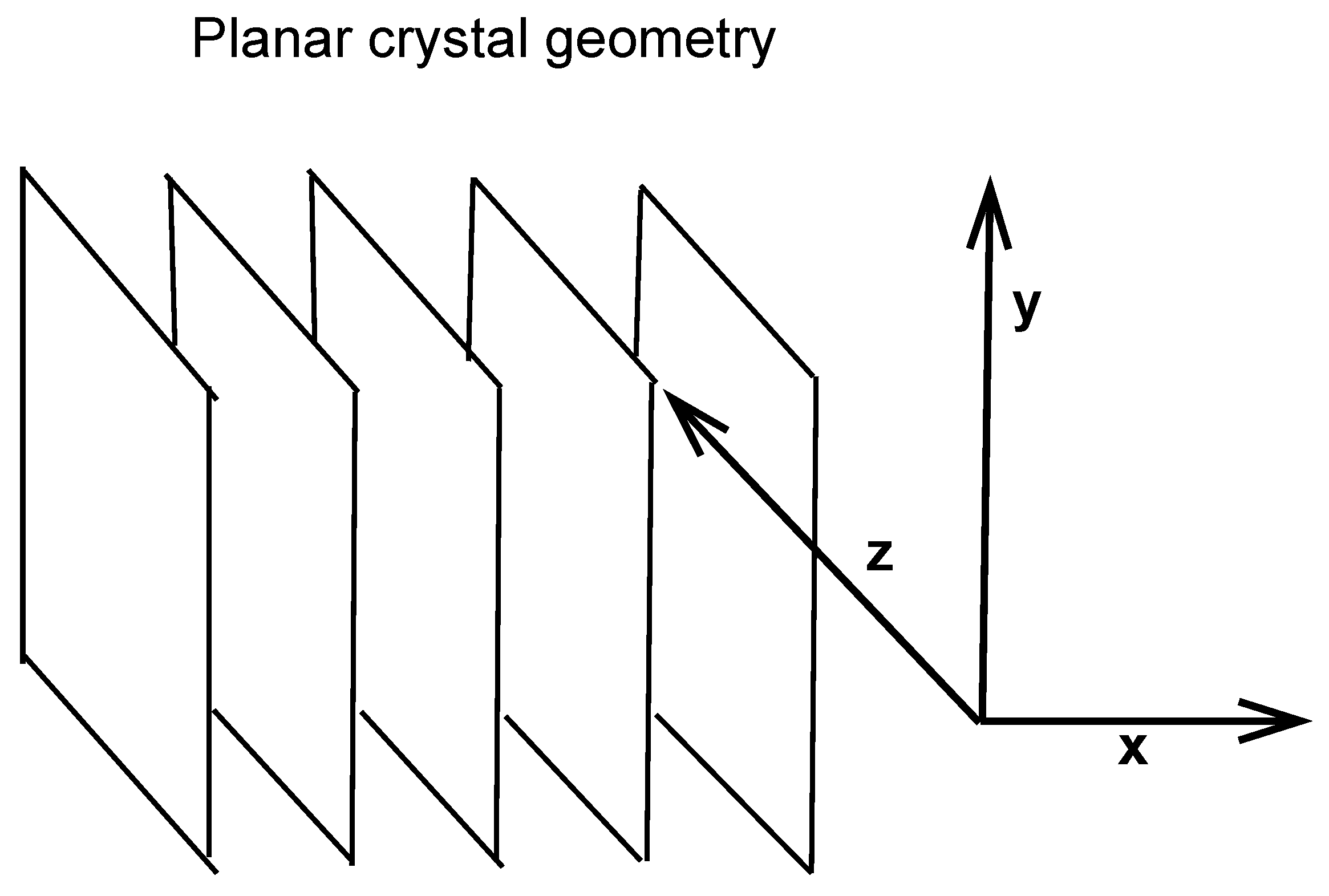
1.5. Form and Parameters of the Target Structure

For this exploratory paper, we assume a simplified planar structure as in Figure 1 for the absorbing regions. The absorption properties of the target are organized according to parallel planes. They are described by an optical potential, which is homogeneous, moving along a path that is parallel to a plane, and periodic along a path orthogonal to a plane.

Let D be the plane–plane spacing. Each plane is the center of a region of thickness $D-a$ < D, where an antiproton is captured by some ion of the plane and removed from the beam. Thus, a is the “complementary” parameter defining the transverse size of the region transparent to the antiproton crossing.

1.6. Summary of the Paper

In Section 2, we will discuss our main mathematical approximation, that is, a Glauber-style formalism [27,28], that assumes short longitudinal wavelengths with respect to the relevant ranges of the problem, which are all angstrom-sized (0.1 nm). A De Broglie wavelength equal to 0.1 nm means a momentum of 2 keV/c. This is much smaller than any momentum in the energy region 1–1000 eV.

In Section 3, we discuss the case where an antiproton beam with a perfect momentum definition is incident on a crystal exactly along a classical channeling direction that is parallel to the planes and normal to the entrance and exit surfaces of the crystal. The other surfaces play no role, since we consider the crystal to have a larger cross-section than the beam. In Section 3, we consider the more general case where the incidence is not perfectly normal, and in Section 5 we apply the obtained cross-sections to the Monte Carlo simulation of an experiment where a realistic beam (with angular spread) crosses a crystal that is slightly rotated, measuring the final transparency as a function of the crystal orientation. Section 6 is devoted to some questions left open by our treatment, in particular, the form of the mean-field potential and the rather complex mechanisms contributing to it.

2. Glauber Approximation

We use a Glauber-method specialization [27,28] of the semiclassical WKB approximation of the antiproton wave. For a synthetic discussion of the Glauber method, see [17], subsection 131 “high energy scattering”, and [29] for a comparison between a wavefunction calculated by the method here employed. By a standard large-L partial wave expansion, see [30] for a comparison with a Monte Carlo calculation and [31] for a comparison between applications of this method to different problems.

2.1. Separation of Longitudinal and Transverse Degrees of Freedom, and Linearization of the Schrödinger Equation

In the WKB semiclassical approximation, the eikonal form of a single particle wavefunction is $e^{i\xi (x,y,z)}$, and the leading approximation for its phase is $\xi (x,y,z)=\overrightarrow{k}(x,y,z)·\overrightarrow{r}$, where $\hslash k(x,y,z)$ is the $local$ classical 3-momentum of the particle, $|\hslash k(x,y,z\left)\right|=\sqrt{E-U(x,y,z)}$.

In the Glauber method, the structure of the problem is further simplified, with a special role of a longitudinal axis z, and the constant initial momentum $\overrightarrow{k}\equiv \widehat{z}p/\hslash$ plays a special role. For the antiproton wave in the scattering environment, we assume the form

$$\psi (x,y,z)\equiv e^{ikz}\varphi (x,y,z)$$

(1)

where $\varphi (x,y,z)$ is slowly changing on the length scale $2\pi /k$. In other words, we have something that is similar to a plane wave, where $\varphi$ is a slow modulation of the $exp\left(ikz\right)$ term.

The basic ground for all that follows is that this writing of the wave function makes sense. We observe that the dominance of $exp\left(ikz\right)$ implies both an axial structure of the problem and a clear past-future orientation along this axis. As explicitly tested in [29], where the Glauber approximation was compared with the results of a standard partial-wave expansion, a key point is the number of partial waves effectively involved, with $L_{max}$∼$Rk$, where R is an effective interaction radius. For example, in the case of a scalar point-like target, we have a pure S-wave problem even in the case of k→∞. A pure S-wave problem can never be reduced to an axial and oriented geometry. Oriented axiality requires at least an S-P wave interference. Of course, the more partial waves are involved, the better.

As we demonstrate later, here, the reference radius is of an atomic size, so the condition $L_{max}$ ≫ 1 means $k{R}_{atom}$ ≫ 1 is satisfied if the wavelength is much shorter than ${10}^{-10}$ m. As previously observed, this is satisfied for p ≫ 1 keV/c corresponding to E ≫ 10⁻³ eV.

Given the above form of Equation (1), the kinetic term in the Schrödinger equation is approximated

$$\begin{array}{cc}\hfill {\nabla }^2+k^2& =\left(\frac{{\partial }^2}{\partial z^2}+k^2\right)+\frac{{\partial }^2}{\partial x^2}+\frac{{\partial }^2}{\partial y^2}=\left(\frac{\partial }{\partial z}-ik\right)\left(\frac{\partial }{\partial z}+ik\right)+\frac{{\partial }^2}{\partial x^2}+\frac{{\partial }^2}{\partial y^2}\end{array}$$

(2)

$$\begin{array}{cc}& \approx 2ik\left(\frac{\partial }{\partial z}-ik\right)+\frac{{\partial }^2}{\partial x^2}+\frac{{\partial }^2}{\partial y^2}\end{array}$$

(3)

$$\begin{array}{cc}& \approx 2ik\left(\frac{\partial }{\partial z}-ik\right)\end{array}$$

(4)

This contains several approximations. In Equation (3), we exploit the requirement of $\varphi$ being a slow modulation in Equation (1):

$$\frac{\partial \psi (x,y,z)}{\partial z}=\frac{\partial \left[\varphi e^{ikz}\right]}{\partial z}\approx \varphi \frac{\partial e^{ikz}}{\partial z}=ik\left(\varphi e^{ikz}\right)$$

(5)

so that

$$\left(\frac{\partial }{\partial z}+ik\right)\left(\varphi e^{ikz}\right)\approx 2ik\left(\varphi e^{ikz}\right)$$

(6)

The residual derivative

$$\left(\frac{\partial }{\partial z}-ik\right)\left(\varphi e^{ikz}\right)=e^{ikz}\frac{\partial \varphi }{\partial z}$$

(7)

singles out the longitudinal deviations of the wavefunction from the leading $exp\left(ikz\right)$ term. In this scheme, reflected waves do not exist. We may only have slightly delayed or slightly advanced waves with respect to the reference oscillation $exp\left(ikz\right)$.

The approximation of Equation (4) neglects ${\partial }^2/\partial x^2$ and ${\partial }^2/\partial y^2$ with respect to the longitudinal term. In the limit $k\to \infty$, this is of course justified by the weighting factor $2ik$, advantaging the longitudinal term over the transverse ones.

2.2. Solution of the Linearized Equation

Summarizing the previous approximations,

$$\left(k^2+{\nabla }^2\right)\left(\varphi e^{ikz}\right)\approx 2ik{e}^{ikz}\frac{\partial \varphi }{\partial z}$$

(8)

We apply this to the Schrödinger equation

$$-{\nabla }^2\left(\varphi e^{ikz}\right)+\frac{2m}{{\hslash }^2}U\left(\varphi e^{ikz}\right)=k^2\left(\varphi e^{ikz}\right)$$

(9)

for an antiproton with beam energy

$$E\equiv \frac{{\hslash }^2{k}^2}{2m}\frac{\partial \varphi }{\partial z}$$

(10)

subject to a complex potential

$$U=U^{\prime }-i{U}^{″}$$

(11)

with $U^{″}$ real and positive, so $Im\left(U\right)$< 0. Using the approximation (8) we obtain the linearized equation for the modulation factor $\varphi (x,y,z)$:

$$\frac{\partial \varphi }{\partial z}=\frac{1}{2ik}\frac{2m}{{\hslash }^2}U\varphi$$

(12)

with solution:

$$\begin{array}{cc}\hfill \varphi (x,y,z)& =exp\left(-i{\int }_{-\infty }^{z}V(x,y,z^{\prime })d{z}^{\prime }\right)\hfill \\ \hfill & =exp\left(-i{\int }_{-\infty }^{z}Re\left(V\right)d{z}^{\prime }\right)+exp\left(-{\int }_{-\infty }^z\left|Im\left(V\right)\right|d{z}^{\prime }\right)\hfill \\ \hfill V& \equiv \frac{m}{{\hslash }^2}\frac{U}{k}\hfill \end{array}$$

(13)

where the integration path is a straight line parallel to z.

We will name V the “optical potential” in the following, although strictly speaking, the potential appearing in the original Schrödinger equation is U.

2.3. Complex Potentials

An optical potential is an effective mean field where all the inelastic processes of the projectile-target interactions are summarized in a regular function $Im\left(V\right)$ associated to the local flux absorption probability, since the actual focus of a researcher is the consequence of these phenomena on one specific channel, in our case, the elastic one. As shown in Section 6, formal ways have been elaborated to build an optical potential from the first principles and a detailed knowledge of the inelastic processes, which is exactly what one wants to bypass. Thus, the historically more common procedure is to infer the general form of the potential from some model hypotheses, respect constraints from the formal theory, and use feedback from the results and fits over the data when available.

The shape of V will be defined in the next section. Its composition and justification are analyzed in detail in Section 6.

The imaginary part of an optical potential is negative, implying a flux absorption: in the time-dependent Schrödinger equation, for V = $-i\left|V\right|$,

$$\begin{array}{c}\hfill i\frac{\partial \psi }{\partial t}=H_0\psi -i\left|V\right|\psi \to \psi \propto e^{-i{E}_{0}t}{e}^{-\left|V\right|t}\end{array}$$

(14)

As anticipated in the Introduction, our strongest assumption is that the local opacity is the only relevant aspect of the antiproton interactions in the elastic channel. In terms of the optical potential, this means a purely imaginary optical potential:

$$V\equiv -i\left|V\right|$$

(15)

What is neglected (see Discussion) are those interactions that do not lead to inelasticity, and whose mean field effect would be expressed as $Re\left(V\right)$.

3. Opacity and Transparency Structure of the Target for Normal Beam Incidence

3.1. Local Probability of Inelasticity

We consider first, an antiproton wave, whose incidence is perfectly orthogonal to the crystal surface.

We imagine the simplest possible target geometry, that is, a crystal with a planar structure, as in Figure 1. As shown in the figure, the planes are parallel to the $yz$-plane, and x is the axis normal to the crystal planes. The antiproton beam axis is the z-axis. Let D be the plane–plane distance.

Let $F(x,y,z)$ be the internal charge density. We approximate it as a function of x only. This means we assume the homogeneity of the structure within each $yz$-parallel plane, apart from the crystal borders at $z=0$ and $z=L$:

$$F(x,y,z)\equiv F\left(x\right)\mathrm{for}z>0\mathrm{and}z<L.$$

(16)

We also assume the periodicity with respect to x, with period D:

$$F(x,y,z)\equiv F\left(x\right)=F(x+nD),$$

(17)

for integer n=$-\infty ,\dots ,+\infty$. For the target, we assume large transverse sizes $L_x$ and $L_y$, which are only needed to avoid divergency problems in later integrations.

We will not directly use the charge density F, but we will use a function describing the $probability$ for any inelastic process that removes an antiproton from its initial state of energy E (capture, inelastic scattering, and so on). This probability is clearly related to F since the leading factor causing the antiproton inelasticity is the Coulomb focusing of the antiproton wave towards the negative charges, triggering inelastic processes (see Section 6).

Let $\rho (x,y,z)$ express the relative probability of the antiproton being removed from the initial state. Let $\lambda$ be the free mean path of an antiproton in the crystal. Then, $\rho (x,y,z)dz/\lambda$ is the actual absorption probability with a correct magnitude when crossing a thickness $dz$. We do not know the relation between F and $\rho$, and the two are not likely to be proportional (since an antiproton is captured when it is near an ion, not necessarily on an ion). However, we may imagine that $\rho$ inherits some properties of F:

• $\rho$ is larger where F is large and positive. This is expressed by a range parameter $|D-a|$: when the $\overline{p}$-plane distance is larger than $|D-a|$, the chances for the antiproton to be captured by the ions of that plane are small. We expect the capture range to be of an atomic scale, similarly to the ion–ion distance D.
• $\rho$ does not depend on y and z, apart form crystal borders at z = 0 and z = L. Thus, we will write $\rho (x,z)\equiv \rho \left(x\right)$, although there is a residual z-dependence, since $\rho$ is zero out of the target.
• $\rho$ is periodic in x with period D.

We will express these properties by writing $\rho \left(x\right)$ as a sum of identical functions ${\rho }_0\left(x\right)$, each associated to a plane:

$$\begin{array}{c}\hfill \rho =\sum _n{\rho }_0[(x-nD)/a],\\ \hfill n=-\infty ,\dots ,+\infty .\\ \hfill {\rho }_0=0\mathrm{for}z<0,z>L.\\ \hfill {\rho }_0(x/a)\approx 1\mathrm{if}\left|x\right|\ll a,\\ \hfill {\rho }_0(x/a)\ll 1\mathrm{if}\left|x\right|\gg a.\end{array}$$

(18)

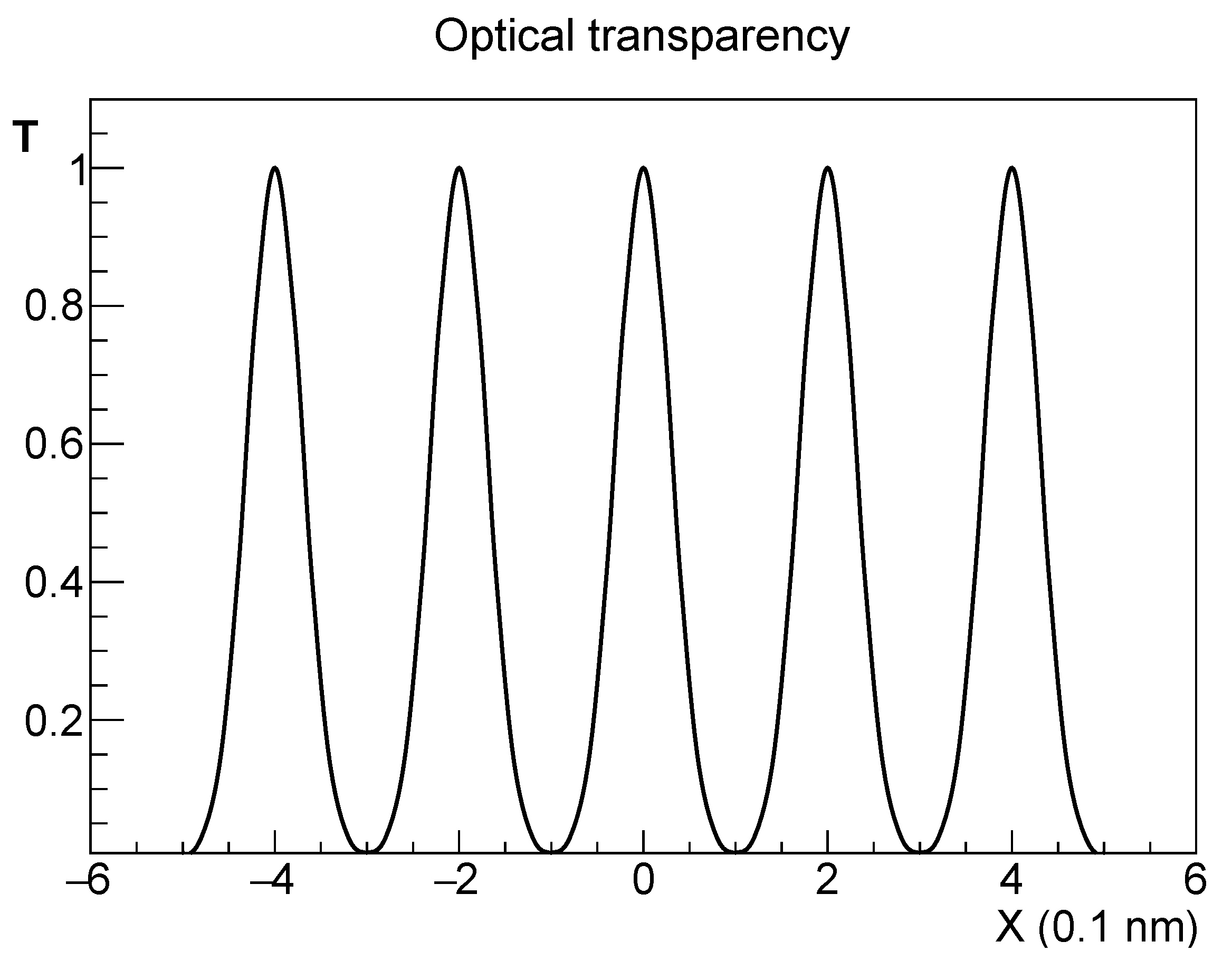
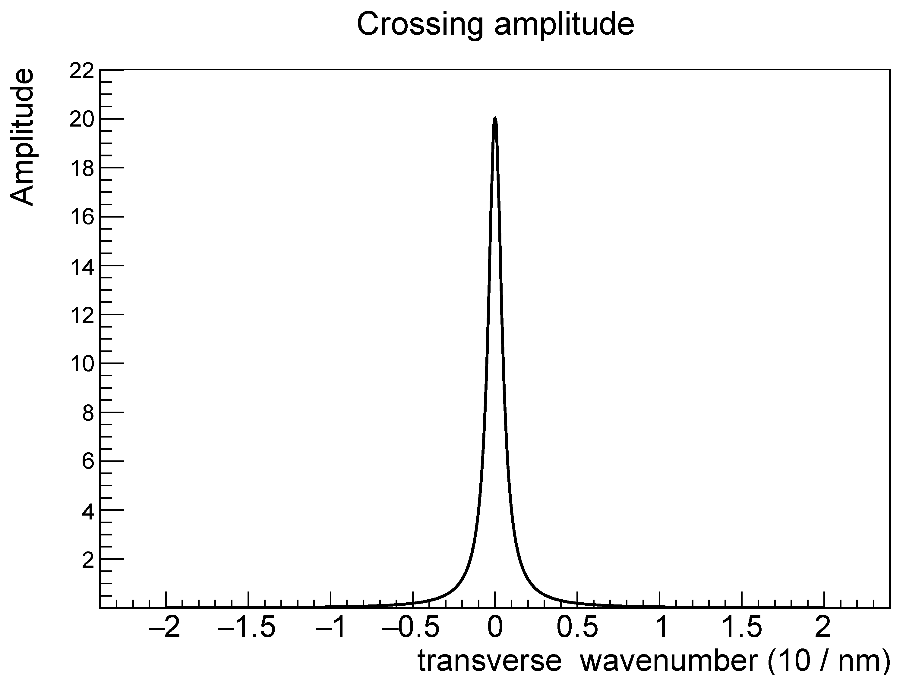
3.2. Optical Potential, Scattering Amplitude and Transparency Factor

The function $\rho$ is a local probability of absorption, not an amplitude. However, using the optical theorem, the optical potential V describing this interaction is imaginary and proportional to $\rho$ (one may considerthe forward scattering amplitude $dA$ from a small volume element $dxdydz$, that in the Born approximation is ∝$Vdxdydz$. Because of the optical theorem, the imaginary part of this amplitude is ∝$d{\sigma }_{tot}$, where the latter refers to the contribution of the volume element only):

$$\begin{array}{c}\hfill V(x,y,z)=-i\sum _n{\lambda }^{-1}\frac{\rho \left[\right(x-nD\left)\right]}{a},\\ \hfill n=-\infty ,\dots ,+\infty .\\ \hfill V(x,y,z)=0\mathrm{for}z<0\mathrm{and}z>L\end{array}$$

(19)

The strength of $V(x,y,z)$ is represented by the dark regions in Figure 2. Clearly, the more the antiproton is midway in between two planes, the more it is likely to survive the crystal crossing. The plane wave describing an antiproton in the empty space is $exp(-ipz)$. According to Equation (13), inside the crystal, the antiproton wave is distorted by an absorption factor

$${\Psi }_p(x,y,z)=e^{-ipz}exp\left(-i{\int }_0^{z}V(x,y,z^{\prime })d{z}^{\prime }\right)$$

(20)

that in our case simplifies to

$${\Psi }_p(x,y,z)={\Psi }_p(x,z)=e^{-ipz}exp\left(-z\left|V\right(x\left)\right|\right)$$

(21)

since V does not depend on y and z, and V = $-i\left|V\right|$.

The scattering amplitude towards a direction ${\overrightarrow{p}}_F$ is

$$\begin{array}{cc}\hfill \langle e^{-i\overrightarrow{p^{\prime }}·\overrightarrow{r}}|{\Psi }_p\rangle & =\frac{1}{L_x{L}_{y}L}\int dxdydz{e}^{-i\overrightarrow{q}·\overrightarrow{r}}exp\left(-z\left|V\right(x\left)\right|\right),\hfill \\ \hfill \overrightarrow{q}& \equiv \overrightarrow{p}-{\overrightarrow{p}}_F\hfill \end{array}$$

(22)

For small angles, $\overrightarrow{q}$ is transverse to the beam, and since the dynamics along y are trivial, we take $\overrightarrow{q}$ as directed along x:

$$\begin{array}{c}\hfill \overrightarrow{p}=(0,0,0),\overrightarrow{q}=(q,0,0),\\ \hfill {\overrightarrow{p}}_F=(-q,0,p),\mathrm{for}q\ll p\end{array}$$

(23)

The scattering angle is

$$\theta =\frac{q}{p}$$

(24)

Since $\overrightarrow{q}$ has no y component, nothing inside the integral depends on y. Thus, the integral in $dy$ simplifies with $1/L_y$, giving 1, and may be omitted in the following. Since $\overrightarrow{q}$ has no z-component, the z-integral may be factorized out of the Fourier transform, and we obtain

$$\langle e^{-i\overrightarrow{p^{\prime }}·\overrightarrow{r}}|{\Psi }_p\rangle =\frac{1}{L_x}\int dx{e}^{-iqx}S\left(x\right)$$

(25)

where the “transparency factor” $S\left(x\right)$ is

$$S\left(x\right)=\frac{1}{L}{\int }_0^{L}dz{e}^{-\left|V\right|z}=\frac{1-exp(-|V\left(x\right)\left|L\right)}{\left|V\right(x\left)\right|L}$$

(26)

with relevant thin target and thick target limits

$$S\left(x\right)\approx 1-\frac{\left|V\right(x\left)\right|L}{2},\mathrm{for}L\ll \frac{1}{\left|V\right(x\left)\right|}.$$

(27)

$$S\left(x\right)\approx \frac{1}{\left|V\right(x\left)\right|L},\mathrm{for}L\gg \frac{1}{\left|V\right(x\left)\right|}.$$

(28)

The thick target limit implies that assuming that $V\left(x\right)$ is not really 0, for a L large enough, we obtain $S\left(x\right)$ ≈ 0 for any x. In the opposite case of a sufficiently small L, there are periodic x regions where the $S\left(x\right)$ is non-negligible. These regions act as coherent sources of after-the-crystal antiproton waves. Moreover, this is the case that interests us. The transparency factor $S\left(x\right)$ is the amplitude for crossing the crystal along a straight path parallel to the z axis. This assumes a fixed impact parameter x; thus, it is not a coherent amplitude for crossing the crystal forward or in any other direction. The coherent amplitude is given by the Fourier transform of $S\left(x\right)$. For any choice of $V(x,y,z)$, respecting our initial assumptions (periodicity in x, independence on y and z, decrease over a distance a that is smaller but not much smaller than the plane–plane distance of D), $S\left(x\right)$ must present a qualitative shape, as in Figure 3. Thus, we may directly guess a shape for the transparency factor $S\left(x\right)$ that respects these obvious properties. Concerning the average crossing probability, we must remind ourselves that the average transparency depends on the crystal thickness.

For purposes of analytical simplicity, we have chosen the periodic sequence of Gaussian shapes

$$S\left(x\right)=\sum _n{S}_n\left(x\right)$$

(29)

$$S_n\left(x\right)=exp\left(-\frac{{(x-nD)}^2}{2a^2}\right)$$

(30)

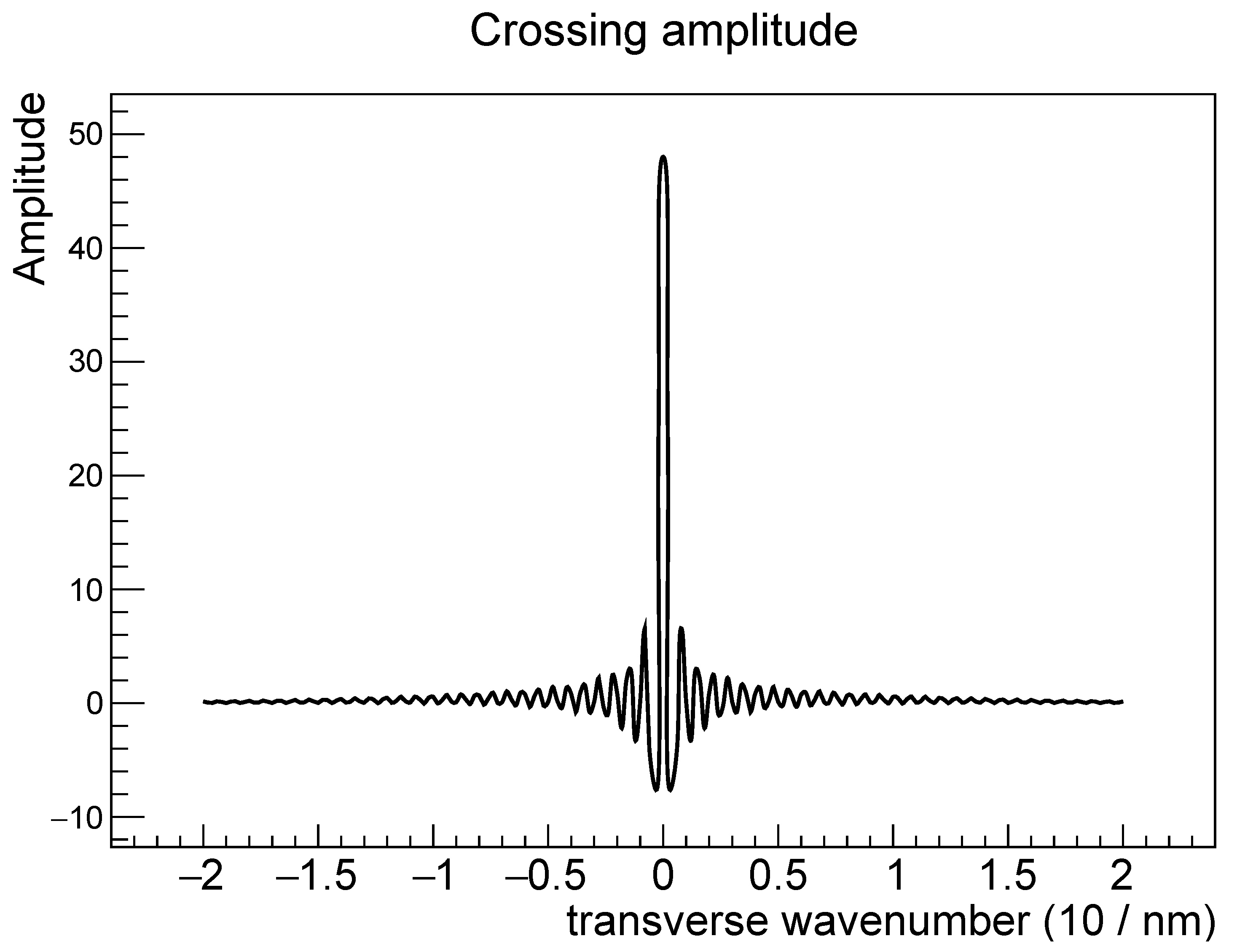
3.3. Beam Coherence and Full-Target Scattering Amplitude

The beam is likely to be an incoherent superposition of wave-packets, each one referring to an individual antiproton. Let $L_c$ be the transverse coherence range of such a wave packet. In other words,

$$\begin{array}{cc}\hfill \left|x\right|\lesssim L_c& \to \mathrm{full}\mathrm{coherence},\hfill \\ \hfill \left|x\right|\gg L_c& \to \mathrm{no}\mathrm{coherence}.\hfill \end{array}$$

(31)

In the following, we will express the loss of coherence in two alternative ways: by the factor

$$C_1\left(n\right)=exp\left(-\frac{{\left(nD\right)}^2}{L_c^2}\right)$$

(32)

in a numerical direct calculation, and by the factor

$$C_2\left(n\right)=exp\left(-\frac{\left|nD\right|}{L_c}\right)$$

(33)

in an analytical calculation. We observe that in the former case, the coherence region is well defined within a range $L_c$, while in the latter, the use of a linear exponential implies a much slower decrease in the coherence when the transverse distance is >$L_c$.

To summarize, apart from an overall constant factor, our scattering amplitude is the Fourier transform (the sum goes from $n=-\infty$ to $+\infty$)

$$\begin{array}{c}\hfill \sum _n{C}_i\left(n\right)\int dx{e}^{-iqx}exp\left(-\frac{{(x-nD)}^2}{2a^2}\right)\\ \hfill =exp\left(-a^2{q}^2\right)\sum _n{C}_i\left(n\right)exp\left(-iqnD\right)\end{array}$$

(34)

We notice that whatever the result of the interference sum, the overall amplitude is suppressed over a scale $\Delta q$ = $1/a$ by the diffraction effect associated with the transverse size a of each transparency channel.

When the coherence length $L_c$ becomes large $L_c$ ≫ D, the predictable result is a central interference line largely overcoming all the secondary interference maxima. Using a moderate $L_c$ = $10D$, this trend is visible already. The results from a direct numerical sum using $C_1\left(n\right)$ are shown in Figure 4, where we have used D = 2 $\mathrm{n}$$\mathrm{m}$, a = 1 $\mathrm{n}$$\mathrm{m}$, and $L_c$ = 20 $\mathrm{n}$$\mathrm{m}$. We have checked that increasing the correlation length $L_c$ leads to a shrinking and growth of the central peak, at the expense of the secondary peaks, tending to a kind of $\delta \left(x\right)$ shape. Using $C_2\left(n\right)$, the sum from $-\infty$ to $+\infty$ may be written in the form

$$\sum _{-\infty }^{+\infty }{f}_n=\sum _0^{\infty }{f}_n+\sum _0^{\infty }{f}_{-n}-1.$$

(35)

$$f_n=e^{inqD}{e}^{-\left|n\right|D/L_c}\equiv {\left(f_1\right)}^n\mathrm{or}{\left(f_{-1}\right)}^n$$

(36)

thus, we may use the known sum rule

$$\sum _0^{\infty }{\xi }^n=\frac{1}{1-\xi }$$

(37)

to calculate both sums. The results, with the same parameters of the numerical case, are shown in Figure 5. Here, secondary maxima are not visible at all (substituting a Gaussian coherence with a linear-exponent coherence means softening the borders of the coherence region).

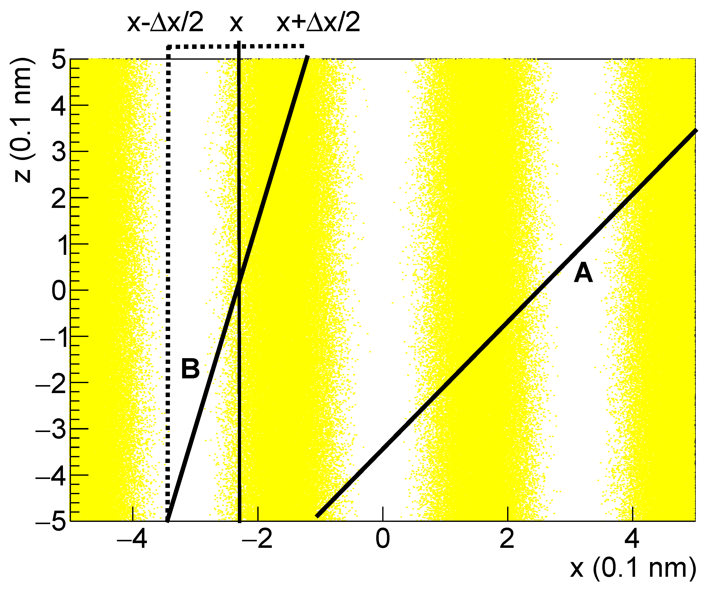
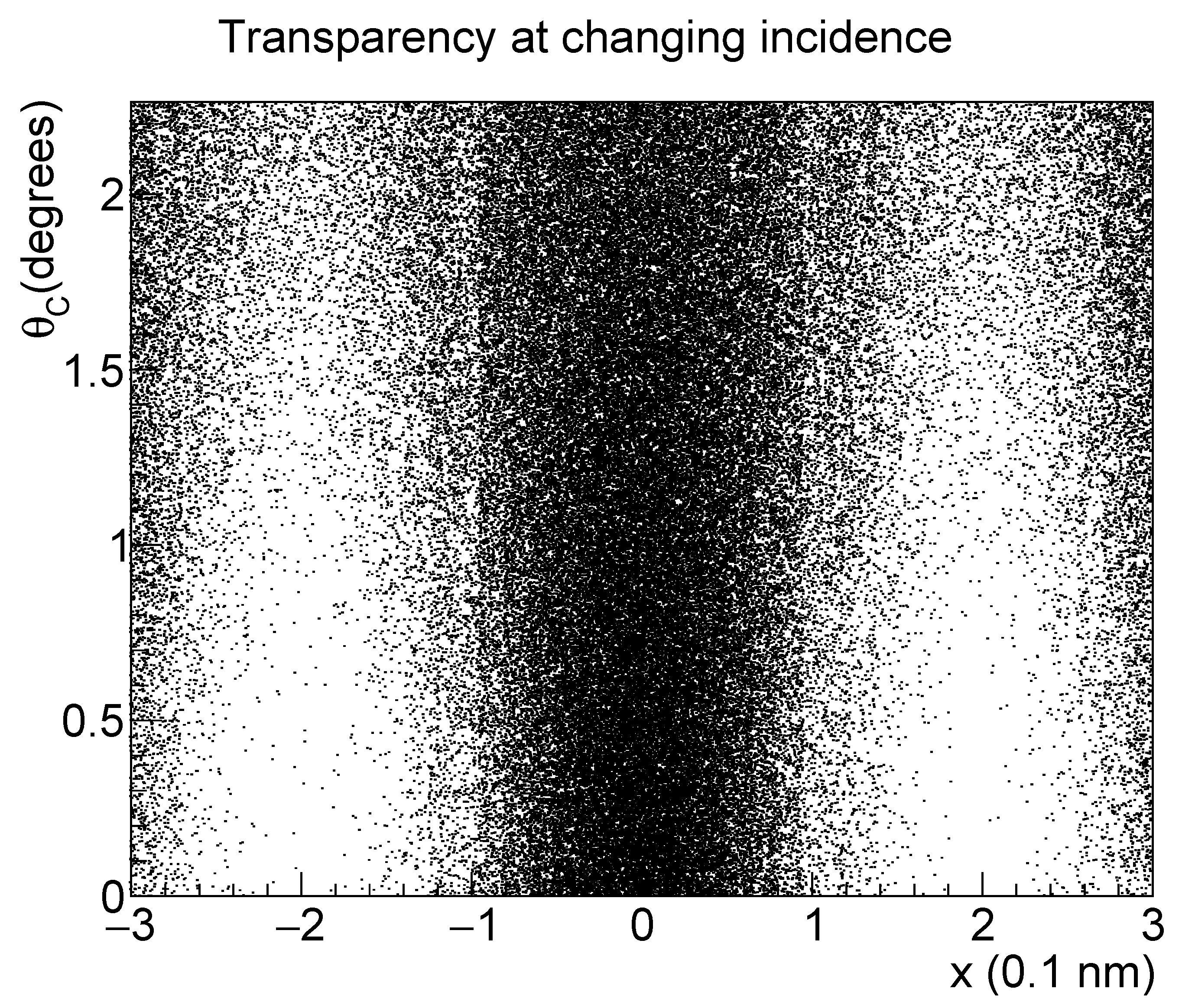
4. Opacity and Transparency; Not Normal Incidence

Since $V(x,y,z)$ does not depend on z and y, the exponential integral defining the transparency $S\left(x\right)$ is trivial when calculated on a straight line parallel to the crystal symmetry axis z. We now consider the more general case, where the initial incidence is rotated by a small angle ${\theta }_C$ on the $xz$ plane. Thus, the incidence vector is

$$\widehat{n}=({\theta }_C,0,1),\left|\widehat{n}\right|\approx 1\mathrm{for}{\theta }_C\ll 1.$$

(38)

$S\left(x\right)$ must be calculated along a straight line with components

$$\begin{array}{c}\hfill \Delta z=L\\ \hfill \Delta x=L{\theta }_C\end{array}$$

(39)

Let $S({\theta }_C,x)$ be the modified transparency calculated along this path. This is illustrated in Figure 6, for the cases of two different paths, with smaller and larger ${\theta }_C$.

If $\theta$ ≫ ${\theta }_{limit}$, where the latter is the largest angle allowing a straight path never to cross an ion plane, the integration trajectory crosses several regions with maximum and minimum absorption. This is the case of trajectory A in the figure. In this limit, $S({\theta }_C,x)$ is the average transparency amplitude $\langle S_L\rangle$∝$exp(-L/2\lambda )$ of the crystal along a randomly oriented path of length ≈ L (it is actually longer because the crystal is not crossed normally, but we assume that the angles are not so large to make this difference relevant, although in the figure the angles are exaggerated for visual purposes). There will be small differences related to the precise periodicity of the crossed maxima and minima of opacity, but not that much; thus

$$S({\theta }_C,x)\approx \langle S_L\rangle \mathrm{for}{\theta }_C\gg {\theta }_{limit}$$

(40)

On the contrary, for small ${\theta }_C$ ≲ ${\theta }_{limit}$ the transverse part $\Delta x$ of the trajectory averages $S\left(x\right)$ over a transverse range $\{x-\Delta x/2,x+\Delta x/2\}$. This is the case of trajectory B in the figure.

$$\begin{array}{c}\hfill S({\theta }_C,x)=\frac{1}{\Delta x}{\int }_1^{2}S\left(x^{\prime }\right)d{x}^{\prime }\\ \hfill “1”=x-\Delta x/2\\ \hfill “2”=x+\Delta x/2.\end{array}$$

(41)

For a simpler calculation, we substitute the clear-cut average with a Gaussian average:

$$\begin{array}{c}\hfill S({\theta }_C,x)\approx \frac{1}{\Delta x}{\int }_{-\infty }^{\infty }S\left(x^{\prime }\right)e^{-\frac{(x-{x^{\prime }}^2)}{2{(\Delta x)}^2}}d{x}^{\prime }\\ \hfill \approx \frac{1}{\Delta x}{\int }_{-\infty }^{\infty }{S}_0\left(x^{\prime }\right)e^{-\frac{(x-{x^{\prime }}^2)}{2{(\Delta x)}^2}}d{x}^{\prime }\\ \hfill =\frac{1}{\Delta x}{\int }_{-\infty }^{\infty }{e}^{-\frac{x^2}{2a^2}}{e}^{-\frac{(x-{x^{\prime }}^2)}{2{(\Delta x)}^2}}d{x}^{\prime }\end{array}$$

(42)

where we begin by only using one of the Gaussian terms defining $S\left(x\right)$ in Equation (29). The final $S({\theta }_C,x)$ will be the sum of all such terms, as in Equation (29), to conserve the x-periodicity of the structure, although only one or two terms are relevant in the case of small angles. As known from standard statistics, the convolution of two Gaussian distributions is just a new Gaussian distribution with a combined width

$$a_C^2=a^2+{(\Delta x)}^2=a^2+{\theta }_C^2{L}^2$$

(43)

while the $1/\Delta x$ normalization factor of the average is $\frac{a}{a_C}$, with limits

$$\begin{array}{c}\hfill \frac{a}{a_C}\approx 1\mathrm{for}{\theta }_C\ll a/L\\ \hfill \frac{a}{a_C}\approx \frac{a}{L{\theta }_C}\mathrm{for}{\theta }_C\gg a/L\end{array}$$

(44)

thus, we may now sum over all the terms:

$$S({\theta }_C,x)=\frac{a}{a_C}\sum _n{S}_n({\theta }_C,x)$$

(45)

$$\begin{array}{c}\hfill S_n\left(x\right)=exp\left(-\frac{{(x-nD)}^2}{2a_C^2}\right),\\ \hfill a_C^2=a^2+{(\Delta x)}^2=a^2+{\theta }_C^2{L}^2\end{array}$$

(46)

For small ${\theta }_C$ ≲ ${\theta }_{limit}$, this sum is dominated by one or two terms. For larger angles, many terms will contribute and S will tend to the average random-angle transparency, as previously observed.

$S({\theta }_C,x)$ is qualitatively shown in Figure 7 (it is calculated with unrealistic parameters for visualization purposes). We observe that for large ${\theta }_C$, the transparency amplitude becomes a constant function of x at the average value $\langle S_L\rangle$ corresponding to a thickness L of the target. We assume a measurement, where in these average conditions antiprotons could not pass at all. Now, here is a key point. We have observed that the shape of the curves in Figure 4 and Figure 5 has a strong dependence on the diffraction parameter a. The larger a, the narrower the x- range where $S\left(x\right)$ is large, although this also depends on the transverse coherence length $L_c$ of the beam. For ${\theta }_C$ ≳ $a/L$, in the previous argument, a is substituted by $a_C$ with a consequent narrowing of the modulation peak. Correspondingly, the peak height is reduced by a factor of $a/a_C$. This way, we have something similar to the classical expectation, where projectiles pass if they do not cross an absorbing plane. However, here, we are considering things at the amplitude level.

5. Simulation Results

5.1. Simulated Experiment

We have set up a Monte Carlo method using the previous amplitude (the one with the analytical calculation, using $C_2\left(n\right)$) to simulate a measurement where we have a thin crystal target that can be rotated by an angle ${\theta }_C$. Every antiproton that is able to cross the target is detected. The beam has a small angular spread. We limit ourselves to the simplest observable variable, which is the outcome of antiprotons when the crystal is rotated by a small angle ${\theta }_C$. This means that at the amplitude level, we have to integrate a single antiproton amplitude over all the possible final $\overrightarrow{q}$, and sum at the probabilistic level over a set of possible initial antiproton directions within a beam spread.

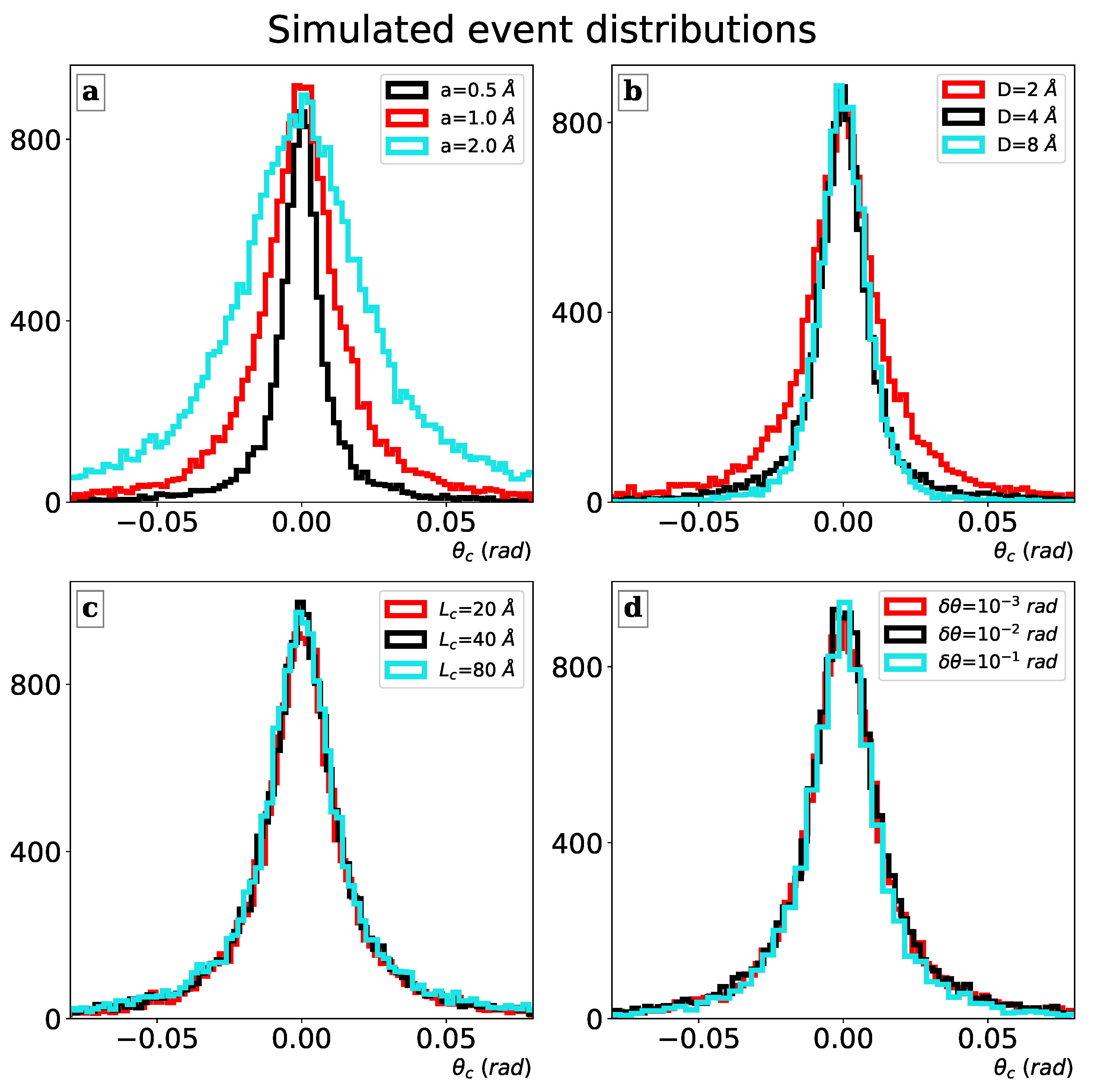
5.2. Simulation Parameters and Systematic Results

In Figure 8, several distributions at the changing parameter values are shown. We have provided the “reference” values of the parameters on the following list:

• A beam with angular width $\delta \theta$ = ±1 mrad.
• A lattice cell size, which in our case means plane–plane spacing: D = 0.2 nm.
• A target thickness L = 8 nm (40 lattice cells).
• A transparency width a = 0.1 nm (half the lattice spacing).
• A beam transverse coherence length $L_c$= 2 nm (this means about 10 planes potentially interfering).

We remark that in our simulations, the overall cross-sections are not comparable, but this is the case for the distribution shapes. Indeed, the overall event number has been chosen each time so as to have the same peak value for each distribution. Due to the simple Gaussian-like shape of the obtained distribution, the most relevant parameter is the half-height width that is of magnitude $0.02$ rad in the reference case.

The parameter changes cover an unrealistic logarithmic range but demonstrate that some parameters have very small effects on the distribution shape.

5.3. Transparency Channel Width

A strong effect is obtained by changing the transparency width a. A further analysis in Figure 9 shows, however, that what is relevant is not a alone, but rather the ratio $a/L$ (L is the crystal thickness). As long as this ratio is constant, the large changes of a do not affect the final results.

5.4. Beam Angular Spread

The distributions do not seriously depend on the beam angular spread in the range $\delta \theta =$ 1–10 mrad. Clearly, the beam spreads ≫ 10 mrad (that is a magnitude of 1 degree) would enlarge the average value of the incident angles and thus reduce the fraction of antiprotons that are able to exploit the channeling range evident in the figure. However, as far as they are below 10 mrad, they do not have a relevant impact on the final outcome.

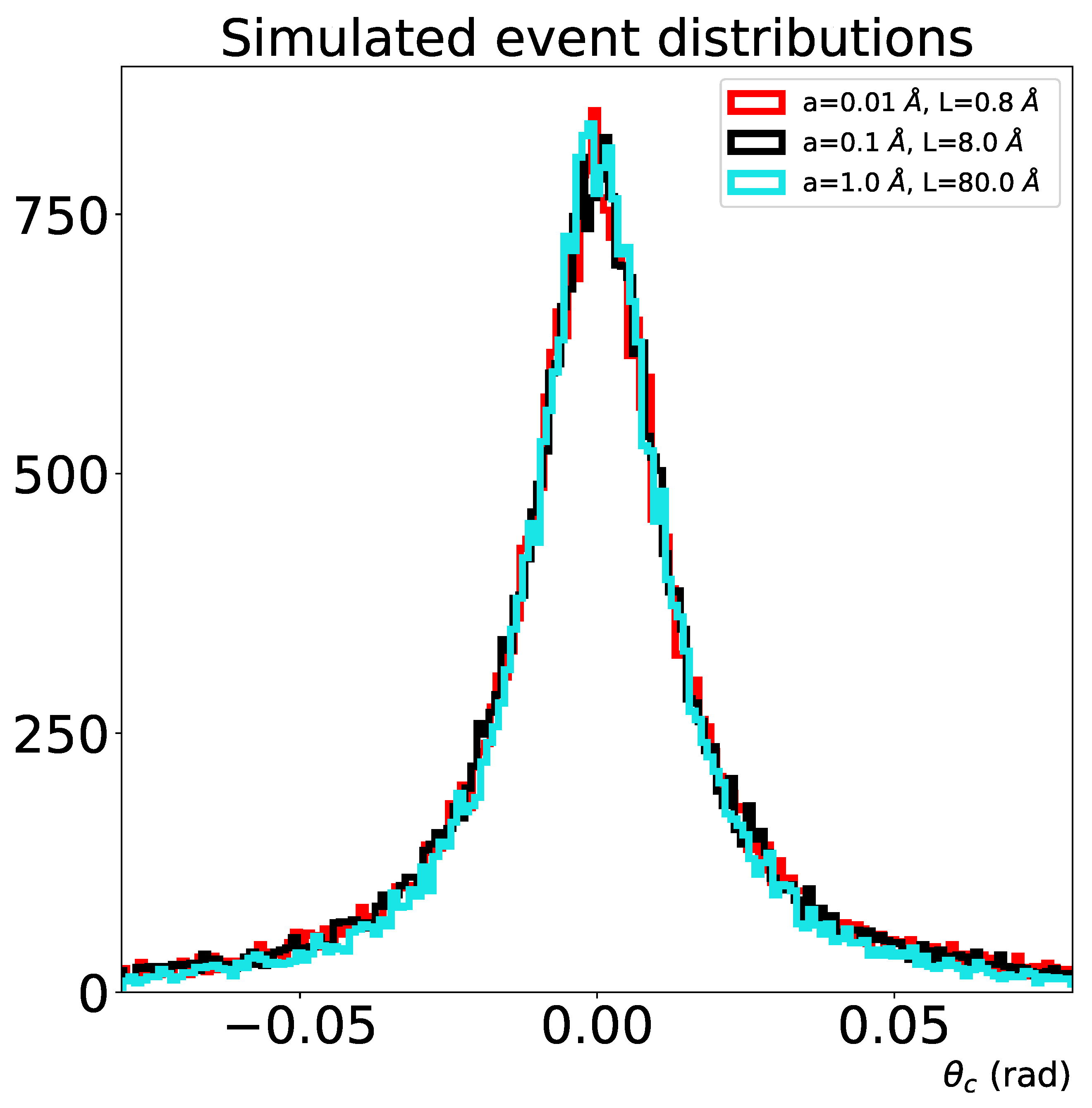
5.5. Correlation Length

The distribution does not depend so much on the correlation length $L_C$ for $L_C$ ranging from one single lattice spacing to 20. This is related to the fast decrease in the a-related diffraction term. This is due to us having used a soft-capture model, where the transparency is a regular function with a scale length a∼D. According to the general rules of the Bragg-like interference from a periodic set of slits, we find multi-peaked structures if a ≪ D, meaning that the slits are thin with respect to their distance. This is not the case here, but in our opinion, it is unrealistic to imagine the existence of thin and sharp transparency channels. A regular transition between opaque and transparent regions, with a relevant role of “grey” transition regions, looks more realistic.

5.6. Target Thickness

The existence of a central channeling peak is related to our hypothesis that some transparency channels do exist. In practical terms, and in agreement with Equation (28), this requires a really thin crystal target, with a thickness of 10–100 lattice cells, although this may depend very much on the specific features of the crystal. A requirement of this work is to be in an absorption-dominated regime. This regime surely exists in a zero-energy limit because in that case even the in-flight annihilation cross-sections (without requiring a previous capture and neglecting the inelastic effects of any other nature) become of a Å${}^2$ magnitude, leaving no room at all for harmless channeling between atoms. However, in this case, the experiment becomes, “by definition”, impossible, unless our target is single-layered or just slightly thicker.

Thus, we imagine a transition energy regime to exist where our assumption of an inelasticity-dominated interaction is justified, but the inelastic antiproton–atom cross-sections are not so large so as to leave no chances for straight-line channeling between atoms. This cannot be much over the keV for the reasons discussed in Section 1. In this regime, although some room for passing through a layer of atoms is left, it cannot be much. Thus, Equation (28), and intuition say that the crystal cannot be too thick.

In Figure 10, we report the outcomes corresponding to different crystal thicknesses. In the case of this figure, the curves present a reciprocally coherent normalization. In other words, in the previous figures, we have for each distribution generated enough events to have the same height for all the peaks. On the contrary, the distributions in Figure 10 are a faithful reproduction of the relative outcomes deriving from the use of crystals of different thicknesses.

As is evident, for thicknesses corresponding to 8 and 40 lattice cells, there is no difference in the peak outcome and little difference at 200 lattice cells. We interpret this as meaning that all the antiprotons have been able to channel at a normal incidence in the first two cases. In the third case, a part of the antiprotons has been absorbed even at a normal incidence; at a thickness of 1000 lattice cells, a very small fraction of antiprotons has survived.

On the other hand, the peaking effect is evidently stronger at a larger thickness, and the width/height ratio decreases at a larger thickness. Thus, depending on the available beam time, it may be a good idea to use crystals that are not exceptionally thin, in order to have more focused final angular distributions. As previously highlighted, the key parameter in this respect is $L/a$. However, since we expect a∼D, $L/D$ is equivalent to $L/a$, and a larger $L/D$ means more absorption and more focusing effects. Thus, a thickness of 100–1000 lattice cells may be a good compromise.

6. Discussion

Our most critical assumption is a small-energy range where it is possible to reduce the antiproton–matter interactions to a mean field imaginary potential. In this section, we discuss this hypothesis in depth.

6.1. General Theory of the Optical Potential

For any theory of the optical potential [32,33,34], the starting point is splitting the space of the projectile+target states into two complementary subspaces, called “elastic” and “inelastic” states, with labels P and Q, respectively. The full problem is projected onto the elastic channel subspace P. This is the subspace of state vectors, where the composite target is in its ground state. The suffix “$PP$” means that the system or an operator, etc., begin from a state of the elastic channel and end in some other state of the elastic channel. “$QP$” refers to transitions from elastic to inelastic, and so on. The problem is finally reduced to a one-body problem, where the projectile in $\overrightarrow{r}$ interacts with a local, complex and energy-dependent potential $V\left(\overrightarrow{r}\right)$ representing the target.

Since a potential may be related to the scattering T-matrix amplitude via a Born approximation (T∼$\int Vexp\left(iqr\right)d^{3}r$), we discuss this in terms of the T-matrix. The formal theory arrives at a reduced scattering operator $T_{PP}$ that only cares about elastic transitions. We write it in an euristic form (see, e.g., Feshbach’s work [32], for the exact form and its elaboration):

$$\langle F|T_{PP}|0\rangle \sim \langle F|T_{elastic}|0\rangle +\sum _n\frac{V_{Fn}{V}_{n0}}{E-E_n+i\eta }$$

(47)

where $|0\rangle$ and $|F\rangle$ are an initial and final state, and both belong to the elastic subspace P, while the states $|n\rangle$ belong to the complementary inelastic subspace Q. $V_{n0}$ and $V_{Fn}$ are matrix elements of $QP$ and $PQ$ projections of the Hamiltonian, and take the system into the inelastic state n and back, but do not allow for the $PP$ and $QQ$ transitions.

The first term $T_{elastic}$ represents the “direct” or “prompt” elastic scattering, where during the process the target is always in its fundamental state. “Prompt” means that the time scale of such a process is the same as for the projectile crossing the target region without interacting.

In the “high energy” treatments introduced in [34], the second term is neglected and the scattering amplitude is calculated as an average over the target ground state $|0_{target}\rangle$ of the projectile-constituent individual interactions:

$$T_{PP}\approx T_{elastic}\equiv \sum \langle 0_{target}|T_{individual}|0_{target}\rangle$$

(48)

where the sum runs over all the constituents of the target.

The second term resembles an ordinary second order perturbative expansion. The elastic $|0\rangle$→$|F\rangle$ transition takes place in two steps $|0\rangle$→$|n\rangle$ →$|F\rangle$, where $|n\rangle$ is a state of the inelastic subspace, for example, a bound state of the projectile and the target. We speak of “delayed” scattering, since the lifetime of this resonance may be much longer than the prompt scattering time, and of “incoherent” scattering, since the final decay into an elastic state has lost any memory of the initial state.

6.2. Imaginary Part of the Optical Potential

The imaginary part of the potential may receive three kinds of contributions.

• Directly from the projectile-constituent scattering amplitude, as in high-energy treatments. Taking the imaginary part of Equation (48):

  $$Im\left(T_{PP}\right)\approx Im\left(T_{elastic}\right)\equiv \sum \langle 0_{target}|Im\left(T_{individual}\right)|0_{target}\rangle$$

  (49)
• From inelasticity at the level of the full projectile+target system, which is the second term in Equation (47). This may contain two kinds of contributions to the imaginary part of $T_{PP}$: (a) discrete resonances of the projectile+target system and (b) continuum fragmentation reactions.
  Discrete resonances are unstable and the $E_n$ factor in Equation (47) is complex with the imaginary part $\Gamma$ = $1/\tau$ being the resonance lifetime.
  Fragmentation states form a continuum; thus, the sum over n is actually an integral bypassing a singularity of the kind

  $$\frac{1}{x_n+i\eta }=P(1/x_n)-i\pi \delta \left(x_n\right),x_n\equiv E-E_n.$$

  (50)
  Integrating the $-i\pi \delta \left(x_n\right)$ term leads to a finite and negative imaginary part of $T_{PP}$ and so of the potential.
• From the loss of coherence:
  The idea (see, e.g., [17], section 145, “Breit-Wigner formulas”) is that although the scattering theory works in terms of states whose energy is infinitely well-defined, a wavepacket realistically reproducing a physical particle is a sum of energy components in a range of “$ϵ$”, which is a range $[E-ϵ/2,E+ϵ/2]$. The wavepacket is destroyed if its components after the scattering present large phase differences within this range. It is customary to define the “optical elastic cross-section” that is calculated from an S-matrix element (S = $1-iT$) that has been averaged in $ϵ$.

  $$S\left(E\right)\equiv \overline{S}\left(E\right)+\delta S\left(E\right),$$

  (51)

  where $\overline{S}\left(E\right)$ is the average of $S\left(E\right)$ in the range $[E-ϵ/2,E+ϵ/2]$ and $\delta S\left(E\right)$ is its fluctuating part. Let us consider S-wave relations as a simple example:

  $$\begin{array}{cc}\hfill {\sigma }_{optical}& \equiv {\sigma }_{el}\left(\overline{S}\right)=\frac{\pi }{k^2}|1-\overline{S}{|}^2={\sigma }_{el}-\frac{\pi }{k^2}{\left|\delta S\right|}^2,\end{array}$$

  (52)

  $$\begin{array}{cc}& {\sigma }_{in}\left(\overline{S}\right)={\sigma }_{in}+\frac{\pi }{k^2}{\left|\delta S\right|}^2.\end{array}$$

  (53)
  The averaging procedure transfers a part of the elastic cross-section into the inelastic one, although the sum ${\sigma }_{tot}$ is unchanged. In terms of amplitude $\overline{S}$ vs. S, we observe that the elastic processes are described by S-elements respecting $\left|S\right|$= 1, which is lying on an Argand circle. Any average of the points of a circle lies inside the circle. Let us consider the limiting case of averaging all the points of the circle: the average is in the center, where $\overline{S}$= 0. This corresponds to

  $$\begin{array}{c}\hfill 0=\overline{S}=1-i\overline{T}\Rightarrow \overline{T}=i\end{array}$$

  (54)

  and is a pure imaginary scattering T-amplitude.

6.3. Low Energy Antiprotons in Matter

The analysis of the antiproton slowing down and annihilating in extremely rarefied monoatomic gases [15], of the same process followed by propagation in the aluminum end wall of the gas vessel, and by the later back-propagation in gas [16], allows for a detailed analysis of the final path of a low-energy antiproton in matter, since the large distance between the target atoms allows for establishing on which atom and when the antiproton ended its path. It shows that in-flight annihilations are a minority, with most antiprotons slowing down initially because of electronic stopping power (down to keV energies) and later for the nuclear stopping power, and finally being captured by an atom. The capture takes place most likely at the antiproton energy 10–100 eV (antiprotons are not found anymore at eV energies) and triggers a cascade process that with a time delay leads the antiprotonic atom to a deeply bound state, where the annihilation takes place [35,36,37,38,39,40]. $\overline{p}$-matter inelasticity cannot only be associated to capture. Any process that seriously affects the target state is inelastic. Of these processes at small energy, we know very little, although common sense suggests that they must have as much statistical weight as the captures (at least).

On this ground, let us try to guess what a mean field optical potential could be, for antiprotons in solid matter in the range of 10–1000 eV.

• Antiproton capture.
  Although very little is known about this process, it is evident that it cannot take place if the (initially positive) energy of the $\overline{p}$ + ion system is conserved. Thus, the capture process must involve three particles, at least. In its most intuitive picture, the antiproton transfers a part of its energy to a deeply bound electron and substitutes it, forming an antiprotonic atom.
  Because of the 1:2000 mass ratio, substituting an electron leaves the antiproton in a large-n and very weakly bound level of the just-formed antiprotonic atom, with a radius that is three orders of magnitude larger than in its fundamental state and in principle even allows for a simultaneous bond with more than one ion, if the replaced electron is a valence one. With small changes of the antiproton–ion initial conditions (energy and impact parameter), we have access to a huge number of such states.
  At the increasing energy, a resonance is described by an S-matrix element S = $\eta exp\left(2i\delta \right)$, with $\eta$ = 1 (elastic resonance) or $\eta$ < 1 (the resonance may decay into inelastic channels), and $\delta$ going from 0 to $\pi$, as the energy ranges from $E-ϵ/2$ to $E+ϵ/2$. An average over the full path falls near the center of the circle, where S = 0 and $Re\left(T\right)$ ≈ 0, $\left|Im\right(T\left)\right|$ $\approx 1$ (S = $1-iT$). In non-averaged scattering, S = 0 corresponds to complete absorption of the incoming flux and sets the unitarity upper limit of the reaction cross-section.
  This is likely to be the most relevant contribution to the imaginary part of the potential at E ≲ 100 eV.
• Close antiproton–ion Coulomb interaction with no capture for E ≲ 100 eV.
  We assume that for E ≲ 100 eV, all the events of this kind fall into the previous class although they do not eventually lead to a captured antiproton.
  Indeed, when an antiproton with a small energy (≲ 100 eV) enters the electronic screening cloud of an ion, its wavefunction has a relevant projection over many large-n antiprotonic atom-bound states. The “borderline” is in the energy denominator $E-E_n+i\eta$ of the second term of Equation (47). It may be near zero (the formation of a long-lived bound state) or finite and large (very virtual intermediate state).
  Although we cannot put a precise upper limit for the capture energy, we assume that the $E_n$ for this process is confined below 100 eV; thus, for E ≫ 100 eV, the factor $E-E_n+i\eta$ suppresses the role of capture states even as virtual states.
• Inelastic processes: E over 100 eV.
  In the capture case, $E_n$ means a huge number of states but still means a discrete set. The lifetime of each captured state is not infinite; thus, it naturally appears in a second-order term as in Equation (47), where eventually (via $V_{Fn}$) the system gets back to the elastic channel.
  Target fragmentation or excitation processes play a role at energies larger than 100 eV. Here, $E_n$ means a continuous set of states.
  As an example, colliding with a 2-atom molecule, an antiproton may remove a valence electron. E is the energy of the “$\overline{p}$+ molecule” system and $E_n$ is the energy of the “$\overline{p}$ + 2 atoms” system), and both are continuous, since neither is a bound system. $E_n$ is real if the final state is stable. Let us assume it is.
  To play a role in Equation (47), this process must get back to the elastic channel: $V_{n0}$ produces the transition, but $V_{Fn}$ reinstates the electron in its place.
  The denominator $E-E_n$ is not obliged to be zero (the state may temporarily exist as a virtual state) but since $E_n$ is real, $Im\left(V\right)$ only comes from the $i\pi \delta$ term in Equation (50), so from the exact singularity E = $E_n$. A pole at a real energy in the second-order term of Equation (47) means two things at the same time:

  (a)

  The system will eventually get back to the elastic channel;

  (b)

  This will take place after an infinite time.

  Point (b) clearly means a complete loss of coherence in the second-step process; thus, near the pole, this term only contributes to $Im\left(V\right)$.
  Far from the pole, we have a contribution to $Re\left(V\right)$ via the $P(1/x_n)$ term in Equation (50)). We observe that for a small virtuality, we have long-lived states, and these are removed by coherence arguments (that is when an energy average is performed, as in Equation (51). High virtuality states are short-lived, but on the other hand, they are suppressed by the energy denominator. Thus, we do not expect a relevant contribution to $Re\left(V\right)$ by these processes.
• Multiple small-angle Coulomb scattering on positive ions (with no role of target-inelastic phenomena).
  Here, we exclude the formation of inelastic target states; thus, a mean field contribution derives from the first term of Equation (47).
  Loss of coherence here does not play a role. Since positive ions are attractive, all the small-angle scattering amplitudes are of the kind S=$exp\left(2i\delta \right)$ with small, real and positive $\delta$ (delay of the scattered wave). Thus,, an energy average over such amplitudes would still be of the kind

  $$\begin{array}{c}\hfill \overline{S}\approx e^{2i\overline{\delta }},\end{array}$$

  (55)

  where the effectively averaged $\overline{\delta }$ is small, real and positive; thus, no relevant $Im\left(V\right)$ derives from this term.
  This argument could change with ionic crystals, where localized concentrations of a negative charge behave as negative ions. We exclude this possibility and assume that we have to use covalent crystals, where stationary electronic distributions only contribute to antiproton scattering via ion screening.
  In principle, the first term of Equation (47) contains all order scattering terms on an individual ion: single, double, etc. If an antiproton is slow and close to an ion, the multiple scattering on it is the rule. At the increasing energy, single scattering becomes more likely, and for large enough energy, we may apply Equation (48), which assumes single scattering. This will lead to a mean-field $real$ potential that is a local sum/average of the Coulomb potentials of all the target charges. This mean-field will coincide with a classically evaluated screened electrostatic potential. Quantum effects on the target side will, however, play a role in a correct estimate of the screening [41].
• Electronic stopping power.
  Electronic long-distance collisions lead to an ordinary stopping power in the Bethe–Bloch sense for energies down to a peak at ∼10–100 keV (see [42,43,44,45,46,47]). Below this peak, the electronic stopping power has been measured to decrease in proportion to the antiproton speed [48] down to 1 keV. Measurements down to $0.5$ keV on light molecules, atoms [49,50] and models [41,51] show that at about 1 keV, the electronic stopping power is very small and is overcome by nuclear stopping power as the main source of energy loss. Extrapolating the data from [49], the data on the propagation of antiprotons in helium and aluminum, down to energies of ∼$10$ eV, were well reproduced in [15,16].
  As far as the average stopping power is considered, one may substitute the leading $exp\left(ipz\right)$ factor in the antiproton wave with $exp\left[ip\right(z\left)\right]$, where $p\left(z\right)$ takes into account the progressive loss of energy. Using, for example the data of [52] for $\overline{p}$ in aluminum, at 1 keV, we have $|dE/dx|$ ≈ 10 eV/$\mathrm{n}$$\mathrm{m}$ (mostly but not entirely of electronic origin). Thus, after 1 $\mathrm{n}$$\mathrm{m}$ of the path, the antiproton passes from 1 keV to $0.99$ keV, meaning a 1% change of its energy. It is a negligible effect.
  Straggling and any kind of statistical dispersion implies $p\left(z\right)$ to have a small imaginary part because of the loss of coherence of the $\overline{p}$ wavefunction. As observed, below 1 keV, the average nuclear stopping power is competitive with the electronic one. Intuitively, we expect it to be far more relevant to statistical dispersion.

6.4. Relevant Energy Thresholds

To summarize this discussion, we assume that for any energy, there will be a critical $\overline{p}$-ion distance. Outside, the potential is the classically screened Coulomb potential. Inside, inelastic phenomena dominate, and the potential is mainly imaginary. This distance is a decreasing function of the energy; thus, at large enough energies, the interaction process is essentially classical, while at small energies, inelasticity takes over. From the previous measurement on the antiproton slowing down in rarefied gases and aluminum, we assume that below 100 keV inelasticity dominates; meanwhile, over 1 keV, the antiproton scattering is dominated by classical electrostatic scattering and the only residual inelasticities are in-flight annihilations with fermi-sized cross-sections. For this reason, the upper energy limit of the validity of our assumption of imaginary dominance is somewhere between 100 and 1000 eV, specifically depending on the target features.

7. Conclusions

We have considered a well-collimated beam (spread ≲ 10 mrad∼ 1 degree) of low-energy antiprotons’ (sub-keV energies), incidence on a very thin crystal (thickness of 10–100 lattice cells). The default beam incidence is normal, but the crystal is rotated by small angles and the overall number of antiprotons crossing the target is predicted as a function of the angle. The crystal structure has been approximated by a periodic planar structure. We have not considered a specific case, but rather assumed some ranges for the relevant parameters, such as cell spacing, thickness or beam spread. Within broad ranges of these parameters, the results are qualitatively stable.

We have assumed that the leading interaction between the antiproton and a crystal atom is a flux absorption with cross-sections of an atomic size. In other words, we have assumed that from a classical point of view, either an antiproton trajectory is undeflected, or any deflection will lead to inelasticity. From previous measurements on the antiproton slowing down and capture and from theoretical arguments, we find it reasonable to assume that an absorption regime dominates below 100 eV and a classical scattering regime dominates over 1 keV, with a progressive transition depending on the target details.

From a wave mechanics perspective, this absorption implies some elastic scattering due to diffraction.

The overall target model is an optical wave absorber with a one-dimensional grid structure and soft transition between the regions, where the waves are stopped or allowed to go.

The final result is that within a small rotation angle, depending on the problem parameters, the antiprotons are allowed to pass with a much larger probability than with an amorphous target with the same average stopping power. This angle may be smaller than the beam spread; thus, we may speak of the focusing (or filtering) effect.

Within the assumptions of the present work, the diffraction effects dominate over interference; thus, we find that a single central channeling peak is the most visible effect of the crystal structure. Secondary interference peaks are not forbidden but are not very visible. Special structures with a sharp transition between transparent and opaque regions could enhance the visibility of secondary Bragg-like peaks. The key point is to have thin and well-defined periodic regions that are sources of crossing antiprotons, but the most likely situation is the one considered here, which is a soft transition between opaque and transparent regions.

To continue the present work, our next step will be to consider a structure with individual absorption centers and, as traditionally studied with classical channeling, decide to which extent and under which conditions it is licit to substitute this ordered set of atoms with continuous mean-field structures, such as the ones used in this work.

References

1. Bandiera, L.; Tikhomirov, V.V.; Romagnoni, M.; Argiolas, N.; Bagli, E.; Ballerini, G.; Berra, A.; Brizzolari, C.; Camattari, R.; De Salvador, D.; et al. Strong Reduction of the Effective Radiation Length in an Axially Oriented Scintillator Crystal. Phys. Rev. Lett. 2018, 121, 021603. [Google Scholar] [CrossRef] [Green Version]
2. Lindhard, J. Motion of swift charged particles, as influenced by strings of atoms in crystals. Phys. Lett. 1964, 12, 126–128. [Google Scholar] [CrossRef]
3. Andersen, J. Notes on Channelling. Available online: https://phys.au.dk/fileadmin/site_files/publikationer/Lecture_notes/Channeling_notes_2018.pdf (accessed on 22 November 2022).
4. Uggerhøj, U.; Bluhme, H.; Knudsen, H.; Møller, S.; Uggerhøj, E.; Morenzoni, E.; Scheidenberger, C. Channeling of antiprotons. Nucl. Instrum. Methods Phys. Res. Sect. B Beam Interact. Mater. Atoms 2003, 207, 402–408. [Google Scholar] [CrossRef]
5. Uggerhøj, E. Some Energy-Loss and Channeling Phenomena for GeV Particles. Phys. Scr. 1983, 28, 331–348. [Google Scholar] [CrossRef]
6. Kuroda, N.; Torii, H.A.; Nagata, Y.; Shibata, M.; Enomoto, Y.; Imao, H.; Kanai, Y.; Hori, M.; Saitoh, H.; Higaki, H.; et al. Development of a monoenergetic ultraslow antiproton beam source for high-precision investigation. Phys. Rev. ST Accel. Beams 2012, 15, 024702. [Google Scholar] [CrossRef]
7. Bendiscioli, G.; Kharzeev, D. Antinucleon-nucleon and antinucleon-nucleus interaction. A review of experimental data. Riv. Nuovo Cim. 1994, 17, 1–142. [Google Scholar] [CrossRef]
8. Bianconi, A.; Corradini, M.; Hori, M.; Leali, M.; Lodi Rizzini, E.; Mascagna, V.; Mozzanica, A.; Prest, M.; Vallazza, E.; Venturelli, L.; et al. Measurement of the antiproton–nucleus annihilation cross section at 5.3 MeV. Phys. Lett. B 2011, 704, 461–466. [Google Scholar] [CrossRef] [Green Version]
9. Aghai-Khozani, H.; Barna, D.; Corradini, M.; Hayano, R.; Hori, M.; Kobayashi, T.; Leali, M.; Lodi-Rizzini, E.; Mascagna, V.; Prest, M.; et al. First experimental detection of antiproton in-flight annihilation on nuclei at ∼130 keV. Eur. Phys. J. Plus 2012, 127. [Google Scholar] [CrossRef] [Green Version]
10. Aghai-Khozani, H.; Barna, D.; Corradini , M.; De Salvador, D.; Hayano, R.; Hori, M.; Kobayashi, T.; Leali, M.; Lodi-Rizzini, E.; Mascagna, V.; et al. First measurement of the antiproton-nucleus annihilation cross section at 125 keV. Hyperfine Interact. 2015, 234, 85–92. [Google Scholar] [CrossRef]
11. Aghai-Khozani, H.; Bianconi, A.; Corradini, M.; Hayano, R.; Hori, M.; Leali, M.; Lodi Rizzini, E.; Mascagna, V.; Murakami, Y.; Prest, M.; et al. Measurement of the antiproton–nucleus annihilation cross-section at low energy. Nucl. Phys. A 2018, 970, 366–378. [Google Scholar] [CrossRef] [Green Version]
12. Aghai-Khozani, H.; Barna, D.; Corradini, M.; De Salvador, D.; Hayano, R.; Hori, M.; Leali, M.; Lodi-Rizzini, E.; Mascagna, V.; Prest, M.; et al. Limits on antiproton-nuclei annihilation cross sections at ∼125 keV. Nucl. Phys. A 2021, 1009, 122170. [Google Scholar] [CrossRef]
13. Friedman, E. Antineutron and antiproton nuclear interactions at very low energies. Nucl. Phys. A 2014, 925, 141–149. [Google Scholar] [CrossRef] [Green Version]
14. Bianconi, A.; Lodi Rizzini, E.; Mascagna, V.; Venturelli, L. Enhancement of annihilation cross sections by electric interactions between the antineutron and the field of a large nucleus. Eur. Phys. J. A 2014, 50, 182. [Google Scholar] [CrossRef] [Green Version]
15. Bianconi, A.; Corradini, M.; Donzella, A.; Leali, M.; Lodi Rizzini, E.; Venturelli, L.; Zurlo, N.; Bargiotti, M.; Bertin, A.; Bruschi, M.; et al. Antiproton slowing down, capture, and decay in low-pressure helium gas. Phys. Rev. A 2004, 70, 032501. [Google Scholar] [CrossRef]
16. Bianconi, A.; Corradini, M.; Cristiano, A.; Leali, M.; Lodi Rizzini, E.; Venturelli, L.; Zurlo, N.; Donà, R. Experimental evidence of antiproton reflection by a solid surface. Phys. Rev. A 2008, 78, 022506. [Google Scholar] [CrossRef] [Green Version]
17. Landau, L.D.; Lifshitz, E.M. Quantum Mechanics—NONRELATIVISTIC Theory; Pergamon Press: Oxford, UK, 1965. [Google Scholar]
18. Cohen, J.S. Molecular effects on antiproton capture by H2 and the states of p¯p formed. Phys. Rev. A 1997, 56, 3583–3596. [Google Scholar] [CrossRef]
19. Révai, J.; Belyaev, V.B. Search for long-lived states in antiprotonic lithium. Phys. Rev. A 2003, 67, 032507. [Google Scholar] [CrossRef] [Green Version]
20. Beck, W.A.; Wilets, L.; Alberg, M.A. Semiclassical description of antiproton capture on atomic helium. Phys. Rev. A 1993, 48, 2779–2785. [Google Scholar] [CrossRef] [Green Version]
21. Bianconi, A.; Charlton, M.; Lodi Rizzini, E.; Mascagna, V.; Venturelli, L. Antiparticle cloud temperatures for antihydrogen experiments. Phys. Rev. A 2017, 96, 013418. [Google Scholar] [CrossRef] [Green Version]
22. Jonsell, S. Collisions involving antiprotons and antihydrogen: An overview. Phil. Trans. Roy. Soc. Lond. A 2018, 376, 20170271. [Google Scholar] [CrossRef] [Green Version]
23. McMorran, B.; Cronin, A.D. Model for partial coherence and wavefront curvature in grating interferometers. Phys. Rev. A 2008, 78, 013601. [Google Scholar] [CrossRef]
24. McMorran, B.; Cronin, A. Gaussian Schell Source as Model for Slit-Collimated Atomic and Molecular Beams. arXiv 2008, arXiv:0804.1162. [Google Scholar]
25. Sala, S.; Ariga, A.; Ereditato, A.; Ferragut, R.; Giammarchi, M.; Leone, M.; Pistillo, C.; Scampoli, P. First demonstration of antimatter wave interferometry. Sci. Adv. 2019, 5, eaav7610. [Google Scholar] [CrossRef] [PubMed] [Green Version]
26. Todoroki, K.; Barna, D.; Hayano, R.; Aghai-Khozani, H.; Sótér, A.; Corradini, M.; Leali, M.; Lodi-Rizzini, E.; Mascagna, V.; Venturelli, L.; et al. Instrumentation for measurement of in-flight annihilations of 130 keV antiprotons on thin target foils. Nucl. Instrum. Methods Phys. Res. Sect. A Accel. Spectrom. Detect. Assoc. Equip. 2016, 835, 110–118. [Google Scholar] [CrossRef]
27. Glauber, R. Lectures in Theoretical Physics; W. Brittain and L.G.Dunham. Interscience Publ.: New York, NY, USA, 1959; Volume 1. [Google Scholar]
28. Glauber, R.; Matthiae, G. High-energy scattering of protons by nuclei. Nucl. Phys. B 1970, 21, 135–157. [Google Scholar] [CrossRef]
29. Bianconi, A.; Radici, M. A test of the eikonal approximation in high-energy (e, e′p) scattering. Phys. Lett. B 1995, 363, 24–28. [Google Scholar] [CrossRef] [Green Version]
30. Golubeva, Y.S.; Kondratyuk, L.A.; Bianconi, A.; Boffi, S.; Radici, M. Nuclear transparency in quasielastic A(e, ep): Intranuclear cascade versus eikonal approximation. Phys. Rev. C 1998, 57, 2618–2627. [Google Scholar] [CrossRef] [Green Version]
31. Bianconi, A.; Radici, M. Angular distributions for knockout and scattering of protons in the eikonal approximation. Phys. Rev. C 1996, 54, 3117–3124. [Google Scholar] [CrossRef] [PubMed] [Green Version]
32. Feshbach, H. A unified theory of nuclear reactions. II. Ann. Phys. 1962, 19, 287–313. [Google Scholar] [CrossRef]
33. Coester, F.; Kümmel, H. Time dependent theory of scattering of nucleons by nuclei. Nucl. Phys. 1958, 9, 225–236. [Google Scholar] [CrossRef]
34. Kerman, A.; McManus, H.; Thaler, R. The scattering of fast nucleons from nuclei. Ann. Phys. 1959, 8, 551–635. [Google Scholar] [CrossRef]
35. Hayano, R.S.; Hori, M.; Horvath, D.; Widmann, E. Antiprotonic helium and CPT invariance. Rep. Prog. Phys. 2007, 70, 1995–2065. [Google Scholar] [CrossRef]
36. Hori, M.; Soter, A.; Barna, D.; Dax, A.; Hayano, R.; Friedreich, S.; Juhasz, B.; Pask, T.; Widmann, E.; Horvath, D.; et al. Two-photon laser spectroscopy of antiprotonic helium and the antiproton-to-electron mass ratio. Nature 2011, 475, 484–488. [Google Scholar] [CrossRef] [Green Version]
37. Hori, M.; Aghai-Khozani, H.; Soter, A.; Barna, D.; Dax, A.; Hayano, R.; Kobayashi, T.; Murakami, Y.; Todoroki, K.; Yamada, H.; et al. Buffer-gas cooling of antiprotonic helium to 1.5 to 1.7 K, and antiproton-to-electron mass ratio. Science 2016, 354, 610–614. [Google Scholar] [CrossRef]
38. Soter, A.; Aghai-Khozani, H.; Barna, D.; Dax, A.; Venturelli, L.; Hori, M. High-resolution laser resonances of antiprotonic helium in superfluid He-4. Nature 2022, 603, 411. [Google Scholar] [CrossRef]
39. Zurlo, N.; Amoretti, M.; Amsler, C.; Bonomi, G.; Carraro, C.; Cesar, C.L.; Charlton, M.; Doser, M.; Fontana, A.; Funakoshi, R.; et al. Evidence for the production of slow antiprotonic hydrogen in vacuum. Phys. Rev. Lett. 2006, 97. [Google Scholar] [CrossRef] [Green Version]
40. Lodi Rizzini, E.; Venturelli, L.; Zurlo, N. On the chemical reaction of matter with antimatter. Chemphyschem 2007, 8, 1145–1150. [Google Scholar] [CrossRef] [PubMed]
41. Nordlund, K.; Sundholm, D.; Pyykkö, P.; Zambrano, D.M.; Djurabekova, F. Nuclear stopping power of antiprotons. Phys. Rev. A 2017, 96, 042717. [Google Scholar] [CrossRef] [Green Version]
42. Borbély, S.; Tong, X.M.; Nagele, S.; Feist, J.; Březinová, I.; Lackner, F.; Nagy, L.; Tokési, K.; Burgdörfer, J. Electron correlations in the antiproton energy-loss distribution in He. Phys. Rev. A 2018, 98, 012707. [Google Scholar] [CrossRef] [Green Version]
43. Abdurakhmanov, I.B.; Kadyrov, A.S.; Bray, I.; Bartschat, K. Wave-packet continuum-discretization approach to single ionization of helium by antiprotons and energetic protons. Phys. Rev. A 2017, 96, 022702. [Google Scholar] [CrossRef] [Green Version]
44. Lüdde, H.J.; Horbatsch, M.; Kirchner, T. Calculation of energy loss in antiproton collisions with many-electron systems using Ehrenfest’s theorem. Phys. Rev. A 2021, 104, 032813. [Google Scholar] [CrossRef]
45. Adamo, A.; Agnello, M.; Balestra, F.; Belli, G.; Bendiscioli, G.; Bertin, A.; Boccaccio, P.; Bonazzola, G.; Bressani, T.; Bruschi, M.; et al. Antiproton Stopping power in hydrogen below 120 keV and the Barkas effect. Phys. Rev. A 1993, 47, 4517–4520. [Google Scholar] [CrossRef] [PubMed] [Green Version]
46. Lodi Rizzini, E.; Bianconi, A.; Bussa, M.; Corradini, M.; Donzella, A.; Venturelli, L.; Bargiotti, M.; Bertin, A.; Bruschi, M.; Capponi, M.; et al. Barkas effect for antiproton stopping in H2. Phys. Rev. Lett. 2002, 89. [Google Scholar] [CrossRef] [PubMed]
47. Lodi Rizzini, E.; Bianconi, A.; Bussa, M.; Corradini, M.; Donzella, A.; Leali, M.; Venturelli, L.; Zurlo, N.; Bargiotti, M.; Bertin, A.; et al. Antiproton stopping power in He in the energy range 1-900 keV and the Barkas effect. Phys. Lett. B 2004, 599, 190–196. [Google Scholar] [CrossRef] [Green Version]
48. Møller, S.P.; Csete, A.; Ichioka, T.; Knudsen, H.; Uggerhøj, U.I.; Andersen, H.H. Antiproton Stopping at Low Energies: Confirmation of Velocity-Proportional Stopping Power. Phys. Rev. Lett. 2002, 88, 193201. [Google Scholar] [CrossRef] [Green Version]
49. Agnello, M.; Belli, G.; Bendiscioli, G.; Bertin, A.; Botta, E.; Bressani, T.; Bruschi, M.; Bussa, M.P.; Busso, L.; Calvo, D.; et al. Antiproton Slowing Down in H2 and He and Evidence of Nuclear Stopping Power. Phys. Rev. Lett. 1995, 74, 371–374. [Google Scholar] [CrossRef]
50. Bertin, A.; Bruschi, M.; Capponi, M.; DAntone, I.; De Castro, S.; Ferretti, A.; Galli, D.; Giacobbe, B.; Marconi, U.; Piccinini, M.; et al. Experimental antiproton nuclear stopping power in H2 and D2. Phys. Rev. A 1996, 54, 5441–5444. [Google Scholar] [CrossRef] [PubMed] [Green Version]
51. Lühr, A.; Saenz, A. Stopping power of antiprotons in H, H2, and He targets. Phys. Rev. A 2009, 79, 042901. [Google Scholar] [CrossRef] [Green Version]
52. Møller, S.P.; Csete, A.; Ichioka, T.; Knudsen, H.; Uggerhøj, U.I.; Andersen, H.H. Stopping Power in Insulators and Metals without Charge Exchange. Phys. Rev. Lett. 2004, 93, 042502. [Google Scholar] [CrossRef] [Green Version]
Figure 1. A 3-dim representation of the approximated crystal structure used in this work. The lattice nuclei are replaced by equal and homogeneous positive charge distributions on the represented planes. The electron charge is distributed in between each pair of planes. The overall charge distribution is periodic with respect to x and does not depend on y and z (inside the crystal border surfaces). The default beam direction is z, although later in this work a small rotation θ C of the incidence angle is considered. The crystal thickness (along z) is L, while L x and L y are the sizes along the other two directions. D is the lattice spacing between planes, while a < D is the width of a transparency channel between nearby planes (see text).
Symmetry 15 00724 g001
Figure 2. The 3-dim representation of the absorbing regions inside a planar crystal.
Symmetry 15 00724 g002
Figure 3. Transparency function, as a function of x; the coordinate that is normal to the absorbing planes.
Symmetry 15 00724 g003
Figure 4. Amplitude for antiproton transmission and numerical calculation with C 1 ( n ) ; see text.
Symmetry 15 00724 g004
Figure 5. Amplitude for antiproton transmission and analytical calculation with C 2 ( n ) ; see text.
Symmetry 15 00724 g005
Figure 6. Trajectories with large (A) and small (B) incidence angle θ C . S ( θ C , x ) is calculated by averaging S ( x ) over the relevant transverse range Δ x , highlighted for trajectory B. In case A, the average involves several alternates of opacity and transparency, and so it roughly coincides with the non-channeled transparency. In case B, the transverse range Δ x only involves one transparency (or opacity) channel.
Symmetry 15 00724 g006
Figure 7. Transparency amplitude S ( θ C , x ) as a function of x and of the incidence angle θ C (that is zero when the antiproton is exactly along the crystal symmetry axis).
Symmetry 15 00724 g007
Figure 8. Simulated event distribution with respect to the crystal rotation angle θ c . In each panel, the red curve is the one with all parameters at reference values (thus, all the red curves are identical). Changing parameters: (a): Transverse size a of the transparency channel (0.1 nm). (b): Lattice spacing (plane-to-plane distance) D (0.1 nm). (c): Transverse correlation length L c (0.1 nm). (d): Beam angular spread δ θ (rad). Remark: the distributions are normalized so as to have coinciding peaks.
Symmetry 15 00724 g008
Figure 9. Simulated event distribution with respect to the crystal rotation angle of θ c . The three curves correspond to very different values of the transparency channel transverse size a and of the crystal longitudinal thickness L, but all correspond to the same value of the a / L ratio. Remark: the distributions are normalized so as to have coinciding peaks.
Symmetry 15 00724 g009
Figure 10. Simulated event distribution with respect to the crystal rotation angle θ c . The curves correspond to very different values of the crystal longitudinal thickness L. The distributions are coherently normalized, that is, they reproduce the relative number of events that we expect at changing thickness.
Symmetry 15 00724 g010
Disclaimer/Publisher’s Note: The statements, opinions and data contained in all publications are solely those of the individual author(s) and contributor(s) and not of MDPI and/or the editor(s). MDPI and/or the editor(s) disclaim responsibility for any injury to people or property resulting from any ideas, methods, instructions or products referred to in the content.