Primordial Gravitational Wave Circuit Complexity

Abstract

In this article, we investigate the various physical implications of quantum circuit complexity using the squeezed state formalism of Primordial Gravitational Waves (PGW). Recently, quantum information-theoretic concepts, such as entanglement entropy and complexity, have played a pivotal role in understanding the dynamics of quantum systems, even in diverse fields such as high-energy physics and cosmology. This paper is devoted to studying the quantum circuit complexity of PGW for various cosmological models, such as de Sitter, inflation, radiation, reheating, matter, bouncing, cyclic and black hole gas models, etc. We compute complexity measures using both Covariance and Nielsen’s wave function method for three different choices of quantum initial vacua: Motta-Allen, $\alpha$ and Bunch–Davies. Besides computing circuit complexity, we also compute the Von Neumann entanglement entropy. By making the comparison between complexity and entanglement entropy, we are able to probe various features regarding the dynamics of evolution for different cosmological models. Because entanglement entropy is independent of the squeezing angle, we are able to understand more details of the system using Nielsen’s measure of complexity, which is dependent on both squeezing parameter and angle. This implies that quantum complexity could indeed be a useful probe to study quantum features on a cosmological scale. Quantum complexity is also becoming a powerful technique to understand the chaotic behaviour and random fluctuations of quantum fields. Using the growth of complexity, we are able to compute the quantum Lyapunov exponent for various cosmological models and comment on its chaotic nature.

1. Introduction

Formally, Gravitational Waves (GW) can be defined as tensor perturbations or disturbances of the space-time metric. Although many indirect evidences for the existence of Gravitational Waves were already available, the first direct detection of Gravitational Waves was made by the Laser Interferometry Gravitational Wave Observatory (LIGO), coming from a black hole merger in 2015 [1]. This has enabled a completely new possibility, in which we can observe our universe along with electromagnetic radiation, neutrino astronomy and others, marking a new era of Gravitational Wave Astronomy.

Once Gravitational Waves are generated, they continue spreading in space-time without interacting with other fields in the universe. If we can detect Gravitational Waves that were formed just after the Big Bang or in very early times, it may potentially reveal information about the very early universe. These Gravitational Waves produced in very early times after the Big Bang are called Primordial Gravitational Waves (PGW). However, because of their relatively very small amplitude, current GW detectors do not have sufficient sensitivity for identifying PGW. As a consequence, some indirect ways of identifying PGW have been suggested using the Cosmic Microwave Background (CMB) power spectrum. The reader can find more detailed aspects in this review and the references therein [2].

Models for the theory of inflation describing early universe cosmology are well-developed. Cosmic Microwave Background measured from COBE in 1989 revealed some irregularities in the temperature map of CMB [3]. Models of inflation can give explanations of such an observation; in fact, the data agree with models of inflation. In the context of quantum field theory of curved space-time, inflation is caused by the inflation field. It is believed that the quantum fluctuations exhibited by the inflation field are responsible for the observed anisotropy in the CMB temperature map. From the recent Planck 2018 observation, we obtain the latest constraints on inflation and the related cosmological parameter estimations, which further constrain the CMB temperature as well as the polarisation maps. See refs. [4,5] for more details.

Primordial quantum fluctuations are thought to be the responsible for inflation [6,7,8,9]. These quantum fluctuations in the early universe are believed to be responsible for the structure of the present-day universe and also the generation of PGW. We analyse these PGW in the form of tensor perturbation in the metric for various cosmological models and then incorporate it with quantum information-theoretic methods, particularly in the computation of quantum circuit complexity. So, the detection of PGW can verify the theory of inflation and also the correctness of the corresponding cosmological model.

Among all inflation models, “Slow roll” is the most widely studied. This model was studied even in the framework of the quantum inverted Harmonic Oscillator system undergoing different phase transitions [10,11,12,13,14]. However, it was found that, at late times, PGW undergo the phenomenon of quantum squeezing, a phenomena widely studied in the context of quantum optics [15]. So, various attempts have been made for identifying the signature for detection of these squeezed PGW. It is argued that the direct detection for such squeezed PGW is not possible; as a result, later on, the possibility of an indirect detection method using Cosmic Microwave Background fluctuations was explored [16,17,18]. The evolution of these PGW can be explained in the framework of quantum squeezing operator formalism [14]. Since there are well-developed quantum information-theoretic tools to study the squeezing operation, we would like to see if we can gain new insights on a cosmological scale using this emerging field of quantum information.

Recently, quantum information theory has became a major factor in various areas of physics. Especially, the calculation of circuit complexity has been paid much attention in recent studies because of its relation with chaos and its possibility to probe physics behind the horizon of black holes in the context of AdS/CFT [19,20,21,22,23,24,25]. Circuit complexity has even been computed in quantum field theories [26,27,28,29,30,31,32]. Despite it being a computational framework, its application has been impactful by giving conjectures such as “Complexity = Action” and “Complexity = Volume” [33,34,35,36].

In the domain of Cosmology, this concept has recently been studied to characterise quantum chaos and complexity in the early universe [37,38,39]. This concept has also been explored in the bouncing cosmological framework and cosmological islands [40,41].

On the other hand, entanglement entropy is also being paid attention in quantum field theory, gravity and cosmology [42,43,44,45,46,47]. It has also been studied as to whether the entanglement entropy has a relation with quantum circuit complexity [48,49,50].

It was realised previously that zero-particle states (vacua) for de Sitter space can exist as transformations according to a set of two parameters for free fields [51,52,53,54]. In relation to that, in this work, we aim to analyse squeezing of PGW with respect to three quantum initial vacuum states: Bunch–Davies, $\alpha$-vacuum and $\alpha -\gamma$ vacuum (also called Motta-Allen vacuum) for various cosmological backgrounds. For this, we first develop a squeezed state formalism for tensor perturbations using circuit complexity and Nielsen’s approach. Then, the Covariance method is calculated. We also give comparisons of entanglement entropy and circuit complexity. Then, we calculate the quantum Lyapunov exponent using these complexity measures.

It is important to note that the latest observational constraint from Planck 2018 was not able to break the degeneracy among various models of inflation, as well as between the bounce and inflationary paradigm at the level of the two-point correlation function (from the amplitude and shape of the spectrum in Fourier space) for the comoving scalar modes. For the tensor modes, only the upper bound of the tensor-to-scalar ratio is available, which is unable to strictly fix the two-point function and its associated power spectrum for PGW in Fourier space. The prime difficulty is as follows: using the present precision level of the cosmological observation, the detection of tensor modes and relics of PGW is very difficult. Moreover, the latest observational probes are unable to detect signatures of non-Gaussianity from the spectrum of higher point correlations using the cosmological perturbed scalar and tensor modes with high statistical precision. Such repeated failure from the various observations in primordial cosmology is one of the strongest motivations to revisit and rethink the overall problem from a completely different perspective. In this work, we use the two-mode squeezed state formalism, with which we quantise the Hamiltonian of the perturbed tensor modes, which, in turn, produces the relics of PGW’ modes in the early universe. In this formalism, we parameterise everything in terms of time-dependent squeezed parameters, which are squeezing amplitude, squeezing angle and an additional phase. These parameters further fix the theoretical structure of two-point or higher quantum correlations, entanglement entropy and quantum circuit complexity. To date, the direct signatures of these parameters or the mentioned derived quantities have not yet been observed in any of the past observational probes of early universe cosmology. From an observational perspective, this is a frustrating fact. However, one should not lose hope by seeing the various findings of quantum information theory within the framework of primordial cosmology. In the near future, instead of probing the amplitude and the power spectrum from two-point as well as higher point functions, if the upcoming cosmological missions are able to measure the previously mentioned squeezing parameters with high statistical accuracy, one will be able to explicitly measure the signatures of various quantum information-theoretic quantities, such as quantum circuit complexity and quantum entanglement, in the cosmological correlation functions. The most probable candidate for this purpose is out-of-time ordered correlation (OTOC), which basically signifies a special type of correlation that can be used to probe the mentioned quantum information-theoretic measures in the context of cosmology. The most significant fact is that, within the framework of primordial cosmological perturbation theory using canonically quantised scalar and tensor modes, one can compute the cosmological version of OTOC in terms of the squeezed state parameters. Because of this specific reason, one can carry forward the computation and make a clear connection between OTOC, quantum circuit complexity and quantum entanglement. Some initial efforts have been already made in a similar direction in refs. [40,41,55,56], where the authors try to establish such connections in various contexts. Even if the signatures of OTOC will not be possible to probe by future cosmological missions, simply measuring the squeezing parameters will still contribute towards the purpose to a great extent. The detection of these parameters through observational probes is not only able to measure the contributions of quantum circuit complexity but also to quantify the amount of quantum entanglement in the cosmological correlations. Such detection will surely help us to distinguish among various models of inflation as well as break the long-standing degeneracy between the bouncing and inflationary paradigms. In this article, we will show in the next sections that just from the PGW (tensor modes) perspective, it is theoretically possible to distinguish among all of these models and paradigms using the quantum complexity measure, which is obviously a good indication, at least from the quantum information-theoretic point of view. This is because, in the context of quantum information theory, quantum circuit complexity is obviously considered the stronger measure compared with quantum entanglement entropy. Within the framework of primordial cosmology, if we can find direct observational evidence of the chaotic signature in terms of the quantum Lyapunov exponent, one would be able to break the degeneracy among various inflationary models, i.e., which one is most probable among inflation and bounce; distinguish reheating and black hole solutions; and open possibilities for many more discoveries. Theoretically, the corresponding measure of the quantum Lyapunov exponent can be computed from the slope of the quantum complexity curves studied with respect to the scale factors computed from various cosmological solutions. We have found from our analysis that not every model can show such features clearly. In the near future, if cosmological observations are able to detect the signature of this effect, it is highly expected that, using the results obtained in this work, one can discard various models and distinguish among various paradigms. In this work, at least from the theoretical point-of-view, we found the same indication, which we will show in the later half of this work. Particularly, the present study with PGW (tensor modes) is extremely important compared with the scalar modes of the perturbation because finding signatures in CMB maps from PGW can tell us about the exact scale of the fundamental physical interactions from which inflationary/bouncing paradigms are created. To date, this is completely a unknown fact. We strongly believe that the present analysis on quantum circuit complexity from the perspective of PGW generated from various cosmological models is able to address at least some of these important unknown facts.

The organisation of the paper is as follows:

• In Section 2, we provide a brief review of quantum circuit complexity and how it can be related to quantum chaos.
• In Section 3, we provide the squeezed state formalism of the cosmological perturbation of PGW. We give a list of various scale factors that we are interested in. As our initial state, we choose different vacua such as the Motta-Allen vacua, $\alpha$ vacua and Bunch–Davies vacua. Finally, we show how the squeezed state formalism in PGW dominated primordial cosmology.
• In Section 4, we compute the quantum circuit complexity of PGW from squeezed states using both Covariance and Nielsen’s wave function approach for all three vacua.
• In Section 5, we compute the entanglement entropy of PGW from squeezed states for each vacua: Motta-Allen vacua, $\alpha$ vacua and Bunch–Davies vacua.
• In Section 6, we perform numerical analyses for various cosmological models. In particular, we compute quantum complexity, entanglement entropy and quantum chaos.
• Finally, in Section 7, we present the concluding remarks and future prospects.

2. Chaos and Complexity: Old Wine in a New Glass

Computationally, circuit complexity is the minimum number of elementary operations required to solve a certain problem. In quantum computation, we can also introduce a similar term that indicates how hard or easy it to solve a particular problem in a quantum computer. In quantum computing, such problems are solved by operations, which can be represented by a unitary transformation. Quantum circuit complexity would then indicate the smallest size of a circuit that implements this unity.

Quantum information-theoretic probes such as entanglement entropy have numerous applications in physics other than quantum computing [57,58]. Very recently, quantum circuit complexity has been gaining attention as one of such tools. One can use quantum circuit complexity to detect topological phases of matter, where a high-complexity quantum state indicates a topological phase. In high-energy physics, quantum complexity is being used to show holographic connections of Anti-de Sitter/Conformal Field Theory (AdS/CFT) correspondence [33,35,36,59]. The “Complexity equals volume” conjecture [33] in the (AdS/CFT) correspondence says that the complexity in the boundary term is proportional to the volume in bulk state. Similarly, the “Complexity equals action” conjecture says that the complexity in the boundary is due to a particular space-time region’s action [34]. Because of these wide motivations, quantum circuit complexity is now being viewed as a powerful tool to study the behaviour of quantum many-body systems. However, computing complexity is a notoriously difficult open challenge. In this section, we will describe the geometric approach introduced by Nielsen [60,61,62,63] to lower bound the circuit complexity.

2.1. Framework of Quantum Circuit Complexity

Let us consider a transformation U, which transforms a reference quantum state ${\psi }_R$ to the target quantum state ${\psi }_T$ and is described by the following equation:

$${\psi }_T=U{\psi }_R$$

(1)

In a quantum computational problem, usually, this unitary transformation U can be written as a sequence of basic unitary gates $Q_i$ that satisfy the constraint

$$\begin{array}{c}\hfill U=Q_1{Q}_2\dots Q_d,\end{array}$$

(2)

where d physically represents the depth of the circuit under consideration. The minimum number of such operations d can be referred to as the circuit complexity. Because it is very difficult to achieve the perfect transformation, we can have the tolerance $ϵ$ such that

$$\left|\right|{\psi }_T-U{\psi }_R{\left|\right|}^2\le ϵ$$

(3)

Nielsen’s approach of computing the complexity is geometric, where the unitary U is constructed using a time-dependent Hamiltonian $H\left(t\right)$:

$$U=\overleftarrow{\mathcal{P}}\exp \left[-i{\int }_0^{1}d\tau H\left(\tau \right)\right]\mathrm{where}H\left(\tau \right)=\sum _I{Y}^I\left(\tau \right){\mathcal{O}}_I$$

(4)

The operator ${\mathcal{O}}_I$ forms a basis for $H\left(\tau \right)$ and $\mathcal{P}$ is a path-ordering operator, which indicates the circuit is moving from left to right. We also need to define a cost function $F(U,\overrightarrow{Y}\left(\tau \right))$, which is a local functional through $U\left(\tau \right)$ and tangent vectors $\overrightarrow{Y}\left(\tau \right)$. The cost for each path is given by

$$\mathcal{D}\left(U\left(t\right)\right)={\int }_0^{1}dtF(U\left(t\right),\dot{U}\left(t\right))$$

(5)

Nielsen showed that using the similar principles of Hamiltonian control theory gives the optimal quantum circuit, where we minimise the functional using a variational approach. There are certain properties we would like the cost function F to satisfy:

• Continuity: Here, we have $F\in C^0$, which implies that we need to consider a continuous cost function. This is expected because of the physical reason.
• Positivity: The continuous cost function should satisfy the constraint $F(U,v)\ge 0$. Here, $F=0$ is obtained from $v=0$. This also means that when this equality condition is satisfied, the reference and target should be same.
• Positive homogeneity: For any positive real number $\alpha$ and any vector v, we obtain $F\left(\alpha v\right)=\alpha F\left(v\right)$.
• Triangle Inequality: The continuous cost function should strictly satisfy the triangle inequality, which is given by $F(U,v+v^{\prime })\le F(U,v)+F(U,v^{\prime }),$ for all tangent vectors v and $v^{\prime }$. Now, if both of these vectors belong to the same ray, the equality holds perfectly.

Here, it is important to note that the definition of the cost function is not unique and, depending on this fact, the quantum complexity measure also changes. These choices are appended below:

$$\begin{array}{c}\hfill \begin{array}{cc}\hfill F_1(U,Y)& =\sum _I\left|Y^I\right|\hfill \\ \hfill F_p(U,Y)& =\sum _I{p}_I\left|Y^I\right|\hfill \\ \hfill F_2(U,Y)& =\sqrt{\sum _I{\left|Y^I\right|}^2}\hfill \\ \hfill F_q(U,Y)& =\sqrt{\sum _I{q}_I{\left|Y^I\right|}^2}\hfill \end{array}\end{array}$$

(6)

Here, $F_1$ represents the linear cost functional measure, which appears from the concept of being closest to the individual counting of gates. Further, $F_2$ represents the quadratic cost functional measure, which appears from the proper distance in the manifold. Next, $F_{1p}$ represents a cost function measure with penalty factors $p_I$ used to favour certain choices over others. Depending on the problem and system we want to study, we will have to choose different cost functions.

In this connection, one can also consider the following possibilities:

$$\begin{array}{cc}\hfill F_k(U,Y)& =\sum _I{\left|Y^I\right|}^k\hfill \\ \hfill F_{\frac{1}{k}}(U,Y)& =\sum _I{\left|Y^I\right|}^{\frac{1}{k}}\hfill \end{array}$$

(7)

where the degree of quantity homogeneity is characterised by $k\ge 1$. These complexities were introduced to match the results from holography such as “Complexity = Action” and “Complexity = Volume” conjectures.

2.2. Quantum Chaos and Complexity

Quantum chaos is a popular tool in many-body quantum physics to study statistical mechanics and thermodynamics [64]. Very recently, it was conjectured that there should be a bound on quantum chaos [65,66] such as

$$\lambda \le 2\pi T$$

(8)

where $\lambda$ is identified to be the quantum Lyapunov exponent and T is the equilibrium temperature of the system. This conjecture was made in the context of holography AdS/CFT [67,68]. Since the complexity of a chaotic system also grows exponentially, one could associate the growth of the complexity measure to the quantum chaos [69]:

$$\lambda =\frac{d\ln \left(C\right[\tau \left]\right)}{d\tau }$$

(9)

where $C\left[\tau \right]$ is the measure of complexity.

3. Squeezed State Formalism of Cosmological Perturbation Theory of PGW

Consider a spatially flat ($k=0$) Friedmann–Lemaître–Robertson–Walker (FLRW) metric in $3+1$ dimensions:

$$\begin{array}{c}\hfill d{s}^2=a^2\left(\tau \right)\left(-d{\tau }^2+d{\mathbf{x}}^2\right)=a^2\left(\tau \right)\left(-d{\tau }^2+{\delta }_{ij}d{x}^{i}d{x}^j\right),\end{array}$$

(10)

where the metric is expressed in a conformally flat form. Here, $a\left(\tau \right)$ is the conformal time-dependent scale factor, which plays the role of the conformal factor in the present context. In this context, conformal and physical time are related via $d\tau =\frac{dt}{a\left(t\right)},$ which is used in the abovementioned expression for the FLRW infinitesimal line element to write it in terms of the conformal time coordinate instead of the physical time coordinate. For this reason, one can treat $t\to \tau ,\mathbf{x}\to \mathbf{x}$ as the coordinate transformation in the present context.

Here, we start with a very simple theory, which is described by

$$\begin{array}{c}\hfill S=\frac{1}{2}\int d^{4}x\sqrt{-g}\left[R-{\left(\partial \varphi \right)}^2-2V\left(\varphi \right)\right],\end{array}$$

(11)

where we fix Planck mass $M_p=1$. Here, $\varphi$ is a scalar field that is minimally coupled to gravity in FLRW space-time. Using this set-up, various types of cosmological solutions of the scale factor can be obtained by solving simultaneously the Friedmann equations and Klein–Gordon equations in a spatially flat FLRW background. Depending on the constraints and structure of the effective potential, all these cosmological solutions can be obtained. In this article, we will not mention any particular class of effective potentials; although, from the cosmological solution of the scale factors, one can predict the features and structures of these effective potentials.

In this section, instead of the effective class of potentials, we are actually interested in the different solutions of the conformal time-dependent scale factors of Friedmann equations, which will finally produce the PGW from the gravitational tensor mode fluctuation. The desired solutions of the scale factors are given as follows:

$$\begin{array}{ccc}\hfill {\displaystyle a\left(\tau \right)}& =& \left\{\begin{array}{cc}{\displaystyle -\frac{1}{H_{*}\tau }}\hfill & \hfill \mathrm{De}\mathrm{Sitter}\\ {\displaystyle -\frac{1}{H_{*}\tau }\left[1+{ϵ}_{*}-{ϵ}_{*}\ln \left(\frac{\tau }{{\tau }_{*}}\right)+\cdots \right]}\hfill & \hfill \mathrm{Inflation}/\mathrm{Quasi}\mathrm{De}\mathrm{Sitter}\left(w\approx -1\right)\\ {\displaystyle {\left[\frac{(1+3w)}{3(1+w)}\tau \right]}^{\frac{2}{(1+3w)}}}\hfill & \hfill {\displaystyle \mathrm{Reheating}\left(0<w<1/3\right)}\\ {\displaystyle \frac{\tau }{2}}\hfill & \hfill \mathrm{Radiation}\left(w=1/3\right)\\ {\displaystyle \frac{{\tau }^2}{9}}\hfill & \hfill \mathrm{Matter}\left(w=0\right)\\ {\displaystyle a_{*}{\left(-\gamma \frac{\tau }{{\tau }_{*}}\right)}^{{\alpha }_{*}}}\hfill & \hfill \mathrm{Contraction}\left(\text{Pre-Bounce}\right)\\ {\displaystyle a_{*}\left[1+{\left(\frac{\tau }{{\tau }_{*}}\right)}^2\right]}\hfill & \hfill \mathrm{Matter}\mathrm{Bounce}\\ {\displaystyle a_{*}\mathrm{sech}\left({\alpha }_{*}(\tau -{\tau }_{*})\right)}\hfill & \hfill \mathrm{Sechyperbolic}\mathrm{Bounce}\\ {\displaystyle a_{*}\cosh \left({\alpha }_{*}(\tau -{\tau }_{*})\right)}\hfill & \hfill \mathrm{Coshyperbolic}\mathrm{Bounce}\\ {\displaystyle a_{*}\sinh \left({\alpha }_{*}(\tau -{\tau }_{*})\right)}\hfill & \hfill \mathrm{Sinhyperbolic}\mathrm{Bounce}\\ {\displaystyle a_{*}\mathrm{cosech}\left({\alpha }_{*}(\tau -{\tau }_{*})\right)}\hfill & \hfill \mathrm{Cosechyperbolic}\mathrm{Bounce}\\ {\displaystyle a_{*}\exp \left(\mathrm{InverseErf}\left({\alpha }_{*}(\tau -{\tau }_{*})\right)\right)}\hfill & \hfill \mathrm{Exponential}\mathrm{Bounce}\\ {\displaystyle a_{*}{\left(\frac{\tau }{{\tau }_{*}}\right)}^{\frac{\alpha }{1-\alpha }}}\hfill & \hfill \text{Power-Law}\mathrm{Bounce}(0<\alpha <1)\\ {\displaystyle a_{*}\sqrt{\gamma \left(\frac{\tau }{{\tau }_{*}}\right)+\delta {\left(\frac{\tau }{{\tau }_{*}}\right)}^2}}\hfill & \hfill \mathrm{Polynomial}\mathrm{Bounce}\\ {\displaystyle a_{*}{\left(\gamma \frac{\tau }{{\tau }_{*}}\right)}^{{\alpha }_{*}}}\hfill & \hfill \mathrm{Expansion}\left(\text{Post-Bounce}\right)\\ {\displaystyle a_{*}\left[1-\cos \left({\alpha }_{*}(\tau -{\tau }_{*})\right)\right]}\hfill & \hfill \mathrm{Matter}\mathrm{Cyclic}\\ {\displaystyle a_{*}\sin \left({\alpha }_{*}(\tau -{\tau }_{*})\right)}\hfill & \hfill \mathrm{Radiation}\mathrm{Cyclic}\\ {\displaystyle a_{*}^{3/2}\exp \left(\frac{i\pi }{2}\right)\sqrt{\frac{2}{3}}{\tau }^{1/2}}\hfill & \hfill \mathrm{Black}\mathrm{Hole}\mathrm{Gas}\end{array}\right.\hfill \end{array}$$

(12)

Most importantly, each of the scale factors carry some information regarding the significant physics of the early universe. We have tried to quote almost all of them available in the cosmology literature. A detailed study on all of these possibilities will give us a complete picture of the underlying physics within the framework of chaos and complexity in our primordial universe. In the rest of the paper, our further objective is to explicitly study all of these possibilities in detail.

3.1. Classical Perturbation Due to PGW

In this section, we will consider only the gravitational contribution, which is basically described by the Einstein–Hilbert term, i.e.,

$$\begin{array}{c}\hfill S_{\mathrm{grav}}=\frac{1}{2}\int d^{4}x\sqrt{-g}R.\end{array}$$

(13)

The production of the PGW is described by the following linearised first-order perturbation in the spatially flat ($k=0$) FLRW metric:

$$\begin{array}{c}\hfill \mathbf{Perturbed}\mathbf{Linearised}\mathbf{Metric}:d{s}^2=a^2\left(\tau \right)\left(-d{\tau }^2+\left({\delta }_{ij}+\underset{\mathbf{Linearised}\mathbf{PGW}}{\underbrace{2h_{ij}(\tau ,\mathbf{x})}}\right)d{x}^{i}d{x}^j\right),\end{array}$$

(14)

where the linearised perturbed PGW or the spin-2 tensor perturbation satisfy the following constraint conditions:

$$\begin{array}{ccc}& & \mathbf{Symmetric}:\Rightarrow h_{ij}=h_{ji},\mathbf{Transverse}:\Rightarrow {\partial }^i{h}_{ij}=0,\mathbf{Traceless}:\Rightarrow h_i^i=0.\hfill \end{array}$$

(15)

Further, by substituting the abovementioned perturbed linearised metric in the Einstein–Hilbert classical gravitational action, the second-order perturbed action is given by

$$\begin{array}{c}\hfill {\delta }^{\left(2\right)}{S}_{\mathrm{grav}}=\frac{1}{8}\int d\tau d^{3}x{a}^2\left(\tau \right)\left[{\left(h_{ij}^{{}^{\prime }}(\tau ,\mathbf{x})\right)}^2-{\left(\nabla h_{ij}(\tau ,\mathbf{x})\right)}^2\right].\end{array}$$

(16)

Further, considering the abovementioned properties of PGW, one can write the following ansatz:

$$\begin{array}{c}\hfill h_{ij}(\tau ,\mathbf{x}):=\sum _{\lambda =+,\times }{h}^{\left(\lambda \right)}\left(\tau \right)e_{ij}^{\left(\lambda \right)}\left(\mathbf{x}\right),\end{array}$$

(17)

where $e_{ij}^{\left(\lambda \right)}\left(\mathbf{x}\right)$ represents the polarisation tensor for PGW for two helicities, $\lambda =+,\times$, respectively.

Next, for computational purposes, it is convenient to define the following rescaled perturbation field variable for the linearised perturbation of PGW, which is given by

$$\begin{array}{c}\hfill \frac{1}{2}a\left(\tau \right)h_{ij}(\tau ,\mathbf{x})\equiv \frac{1}{\sqrt{2}}\left(\begin{array}{ccc}{f}_{(+)}(\tau ,\mathbf{x})& f_{(\times )}(\tau ,\mathbf{x})& 0\\ f_{(\times )}(\tau ,\mathbf{x})& -f_{(+)}(\tau ,\mathbf{x})& 0\\ 0& 0& 0\end{array}\right)\end{array}$$

(18)

which is consistent with all the required constraints on the spin-2 PGW or the tensor perturbation. Using the abovementioned convenient field redefinition, the second-order perturbed action for the linearised tensor modes or the PGW can be written as

$$\begin{array}{c}\hfill {\delta }^{\left(2\right)}{S}_{\mathrm{grav}}=\frac{1}{2}\sum _{\lambda =+,\times }\int d\tau d^{3}x\left[|f_{\lambda }^{{}^{\prime }}{(\tau ,\mathbf{x})|}^2-{\left|\nabla f_{\lambda }(\tau ,\mathbf{x})\right|}^2+\frac{a^{{}^{″}}\left(\tau \right)}{a\left(\tau \right)}{\left|f_{\lambda }(\tau ,\mathbf{x})\right|}^2\right].\end{array}$$

(19)

Now, we transform the above action in the Fourier space using the following equation,

$$\begin{array}{c}\hfill f_{\lambda }(\tau ,\mathbf{x}):=\int \frac{d^3\mathbf{k}}{{\left(2\pi \right)}^3}{f}_{\lambda ,\mathbf{k}}\left(\tau \right)\exp (i\mathbf{k}.\mathbf{x})\forall \lambda =+,\times .\end{array}$$

(20)

Using this further, we obtain

$$\begin{array}{c}\hfill {\delta }^{\left(2\right)}{S}_{\mathrm{grav}}=\frac{1}{2}\sum _{\lambda =+,\times }\int d\tau d^3\mathbf{k}\left[|f_{\lambda ,\mathbf{k}}^{{}^{\prime }}{\left(\tau \right)|}^2-{\omega }^2(k,\tau ){\left|f_{\lambda ,\mathbf{k}}\left(\tau \right)\right|}^2\right],\end{array}$$

(21)

where we define the effective frequency of the PGW a:

$$\begin{array}{c}\hfill {\omega }^2(k,\tau )=k^2+m^2\left(\tau \right)\mathrm{with}\mathrm{effective}\mathrm{mass}{m}^2\left(\tau \right)=-\frac{a^{{}^{″}}\left(\tau \right)}{a\left(\tau \right)}.\end{array}$$

(22)

Further, the Mukhanov–Sasaki equation for PGW can be written as

$$\begin{array}{c}\hfill f_{\lambda ,\mathbf{k}}^{″}\left(\tau \right)+{\omega }^2(k,\tau )f_{\lambda ,\mathbf{k}}\left(\tau \right)=0.\end{array}$$

(23)

Now, the effective mass of the PGW can be further simplified as

$$\begin{array}{ccc}\hfill m^2\left(\tau \right)& =& -\frac{a^{{}^{″}}\left(\tau \right)}{a\left(\tau \right)}=-\left({\mathcal{H}}^2+{\mathcal{H}}^{\prime }\right)=\left(ϵ\left(\tau \right)-2\right){\mathcal{H}}^2,\hfill \end{array}$$

(24)

where we define the slowly varying quantity $ϵ\left(\tau \right)$ as

$$\begin{array}{c}\hfill ϵ\left(\tau \right)=1-\frac{{\mathcal{H}}^{\prime }}{{\mathcal{H}}^2},\mathrm{where}\mathcal{H}=\frac{a^{\prime }\left(\tau \right)}{a\left(\tau \right)}.\end{array}$$

(25)

On the other hand, the mass parameter $\nu \left(\tau \right)$ for PGW can be parameterised as

$$\begin{array}{ccc}\hfill m^2\left(\tau \right)& =& -\frac{1}{{\tau }^2}\left({\nu }_{\mathrm{PGW}}^2\left(\tau \right)-\frac{1}{4}\right),\hfill \end{array}$$

(26)

$$\begin{array}{ccc}\hfill \mathrm{where}{\nu }_{\mathrm{PGW}}\left(\tau \right)& =& \frac{1}{2}\sqrt{1+4{\left(\tau \mathcal{H}\right)}^2(2-ϵ\left(\tau \right))}=\frac{1}{2}\sqrt{1+4{\left(\tau \mathcal{H}\right)}^2\left(1+\frac{{\mathcal{H}}^{\prime }}{{\mathcal{H}}^2}\right)}.\hfill \end{array}$$

(27)

Apart from this, another very crucial quantity plays a significant role to determine the cosmological dynamics, described by

$$\begin{array}{c}\hfill {\mathcal{D}}_{\mathcal{H}}:=\frac{k}{a\left(t\right)H\left(t\right)}=\frac{k}{\mathcal{H}\left(\tau \right)}\to \left\{\begin{array}{cc}{\displaystyle \ll 1}\hfill & \hfill \text{Super-Horizon}\\ {\displaystyle =1,}\hfill & \hfill {\displaystyle \text{Horizon-crossing}}\\ {\displaystyle \gg 1,}\hfill & \hfill \text{Sub-Horizon}\end{array}\right.\end{array}$$

(28)

In the following, we will explicitly derive the expression for the mass parameters and the abovementioned horizon-determining ratio for different primordial universe models:

1.

De Sitter:

$${\nu }_{\mathrm{PGW}}\left(\tau \right)=\frac{3}{2},$$

(29)

$${\mathcal{D}}_{\mathcal{H}}=\frac{k}{\mathcal{H}\left(\tau \right)}=-k\tau .$$

(30)

2.

Inflation/Quasi De Sitter:

$${\nu }_{\mathrm{PGW}}\left(\tau \right)=\frac{3}{2}+3ϵ\left(\tau \right)-\eta \left(\tau \right)\mathrm{with}\eta \left(\tau \right)=2ϵ\left(\tau \right)-\frac{1}{2\mathcal{H}}\frac{{ϵ}^{\prime }\left(\tau \right)}{ϵ\left(\tau \right)},$$

(31)

$${\mathcal{D}}_{\mathcal{H}}=\frac{k}{\mathcal{H}\left(\tau \right)}=-k\tau .$$

(32)

3.

Reheating ($0<w<1/3$):

$${\nu }_{\mathrm{PGW}}\left(\tau \right)=\frac{3}{2}\frac{(w-1)}{(3w+1)},$$

(33)

$${\mathcal{D}}_{\mathcal{H}}=\frac{k}{\mathcal{H}\left(\tau \right)}=\frac{ka\left(\tau \right)}{a^{\prime }\left(\tau \right)}=\frac{1}{2}k\tau (3w+1)$$

(34)

During reheating, the equation of the state parameter lies within the window $0<w<1/3$, which was discussed in detail in refs. [55,70]. However, there is always an ambiguity when having the equation of the state parameter within this prescribed window, as the micro-physics of the epoch of reheating are not known yet and, to date, it was studied from the phenomenological perspective only. Regarding the ambiguity, let us mention ref. [71], where the authors pointed out that during such an epoch the equation of state parameter is $w>1/3$. We have restricted the equation of state parameter within $0<w<1/3$ because it is believed that the classically reheating epoch should lie between matter domination ($w=0$) and radiation ($w=1/3$). The exact form of the equation of state during this epoch is unknown to date.

4.

Radiation ($w=1/3$):

$${\nu }_{\mathrm{PGW}}\left(\tau \right)=-\frac{1}{2}.$$

(35)

$${\mathcal{D}}_{\mathcal{H}}=\frac{k}{\mathcal{H}\left(\tau \right)}=-k\tau .$$

(36)

5.

Matter ($w=0$):

$${\nu }_{\mathrm{PGW}}\left(\tau \right)=-\frac{3}{2}.$$

(37)

$${\mathcal{D}}_{\mathcal{H}}=\frac{k}{\mathcal{H}\left(\tau \right)}=-k\tau .$$

(38)

Bouncing cosmology is emerging as an alternative to inflationary models [72,73,74,75,76,77]. Here, the mass parameters for various bouncing models are given.

6.

Contraction (Pre-Bounce):

$${\nu }_{\mathrm{PGW}}\left(\tau \right)=\alpha -\frac{1}{2}.$$

(39)

$${\mathcal{D}}_{\mathcal{H}}=\frac{k\tau }{{\alpha }_{*}}.$$

(40)

7.

Matter Bounce:

$${\nu }_{\mathrm{PGW}}\left(\tau \right)=\frac{3}{2}\sqrt{1-\frac{8}{9}\frac{1}{\left[1+{\left(\frac{\tau }{{\tau }_{*}}\right)}^2\right]}}.$$

(41)

$${\mathcal{D}}_{\mathcal{H}}=\frac{k({\tau }^2+{\tau }_{*}^2)}{2\tau }.$$

(42)

8.

Sechyperbolic Bounce:

$${\nu }_{\mathrm{PGW}}\left(\tau \right)=\frac{1}{2}\sqrt{1+4{\tau }^2{\alpha }_{*}^2\left[1-2{\mathrm{sech}}^2\left({\alpha }_{*}(\tau -{\tau }_{*})\right)\right]}.$$

(43)

$${\mathcal{D}}_{\mathcal{H}}=\frac{-k\coth \left[{\alpha }_{*}(\tau -{\tau }_{*})\right]}{{\alpha }_{*}}.$$

(44)

9.

Coshyperbolic Bounce:

$${\nu }_{\mathrm{PGW}}\left(\tau \right)=\frac{1}{2}\sqrt{1+4{\tau }^2{\alpha }_{*}^2}.$$

(45)

$${\mathcal{D}}_{\mathcal{H}}=\frac{k\coth \left[{\alpha }_{*}(\tau -{\tau }_{*})\right]}{{\alpha }_{*}}.$$

(46)

10.

Sinhyperbolic Bounce:

In this case, the mass parameter can be evaluated as

$${\nu }_{\mathrm{PGW}}\left(\tau \right)=\frac{1}{2}\sqrt{1+4{\tau }^2{\alpha }_{*}^2}.$$

(47)

$${\mathcal{D}}_{\mathcal{H}}=\frac{k\tanh \left[{\alpha }_{*}(\tau -{\tau }_{*})\right]}{{\alpha }_{*}}.$$

(48)

11.

Cosechyperbolic Bounce:

$${\nu }_{\mathrm{PGW}}\left(\tau \right)=\frac{1}{2}\sqrt{1+4{\tau }^2{\alpha }_{*}^2\left[1+2{\mathrm{cosech}}^2\left({\alpha }_{*}(\tau -{\tau }_{*})\right)\right]}.$$

(49)

$${\mathcal{D}}_{\mathcal{H}}=\frac{k\ast \cos \mathrm{ech}\left[{\alpha }_{*}(\tau -{\tau }_{*})\right]}{{\alpha }_{*}\cos \mathrm{ech}\prime \left[{\alpha }_{*}(\tau -{\tau }_{*})\right]}.$$

(50)

12.

Exponential Bounce:

$${\nu }_{\mathrm{PGW}}\left(\tau \right)=\frac{1}{2}\sqrt{1+\pi {\alpha }_{*}^2{\tau }^2(1+2\mathrm{InverseErf}\left({\alpha }_{*}(\tau -{\tau }_{*})\right))\exp \left(2\mathrm{InverseErf}{\left({\alpha }_{*}(\tau -{\tau }_{*})\right)}^2\right)}.$$

(51)

$${\mathcal{D}}_{\mathcal{H}}=\frac{k}{\mathcal{H}\left(\tau \right)}=\frac{2\exp \left(-\mathrm{InverseErf}{\left[{\alpha }_{*}(\tau -{\tau }_{*})\right]}^2\right)k}{\sqrt{\pi }{\alpha }_{*}}.$$

(52)

13.

Power-Law Bounce ($0<{\alpha }_{*}<1$):

$${\nu }_{\mathrm{PGW}}\left(\tau \right)=\frac{1}{2}\left(\frac{3{\alpha }_{*}-1}{{\alpha }_{*}-1}\right).$$

(53)

$${\mathcal{D}}_{\mathcal{H}}=\frac{(1-{\alpha }_{*})k\tau }{{\alpha }_{*}}$$

(54)

14.

Polynomial Bounce:

$${\nu }_{\mathrm{PGW}}\left(\tau \right)=\frac{1}{2}\frac{1}{({\tau }_{*}\gamma +\delta \tau )}\sqrt{\delta \tau (2{\tau }_{*}\gamma +\delta \tau )}.$$

(55)

$${\mathcal{D}}_{\mathcal{H}}=\frac{2k\tau (\delta \tau +\gamma {\tau }_{*})}{2\delta \tau +\gamma {\tau }_{*}}$$

(56)

15.

Matter Cyclic:

$${\nu }_{\mathrm{PGW}}\left(\tau \right)=\frac{1}{2}\sqrt{1-2{\tau }^2{\alpha }_{*}^2\left[1-{\cot }^2\left(\frac{{\alpha }_{*}(\tau -{\tau }_{*})}{2}\right)\right]}.$$

(57)

$${\mathcal{D}}_{\mathcal{H}}=\frac{k\tan \left(\frac{{\alpha }_{*}}{2}(\tau -{\tau }_{*})\right)}{{\alpha }_{*}}$$

(58)

16.

Radiation Cyclic:

$${\nu }_{\mathrm{PGW}}\left(\tau \right)=\frac{1}{2}\sqrt{1-4{\tau }^2{\alpha }_{*}^2}.$$

(59)

$${\mathcal{D}}_{\mathcal{H}}=\frac{k\tan \left({\alpha }_{*}(\tau -{\tau }_{*})\right)}{{\alpha }_{*}}.$$

(60)

17.

Black Hole Gas:

Black hole gas is a relatively new model that predicts maximum entropy state in the very early universe [78,79,80,81,82]. In this case, the mass parameter and the horizon determining ratio can be evaluated as

$${\nu }_{\mathrm{PGW}}\left(\tau \right)=0$$

(61)

$${\mathcal{D}}_{\mathcal{H}}=\frac{k}{\mathcal{H}\left(\tau \right)}=2k\tau .$$

(62)

We are going to use all of these derived model-dependent expressions for the mass parameters for the PGW during the numerical analysis performed in the later half of this paper. From these derived expressions, it is evident that, depending on the expressions of different models, the expressions for the change in the mass parameter determined in terms of the model parameters. Here, we have found that for some models this parameter is exactly constant and for some classes of models there are appearances of non-trivial conformal time dependence. In the later half of the paper, we will perform the analysis of the squeezed state formalism; from there, we are able to see how these different expressions of the mass parameters will hugely change the dynamical behaviour of the quantum complexity and the related estimators of chaos.

3.2. Classical Mode Function for PGW

For the PGW, the Mukhanov–Sasaki equation is

$$f_{\lambda ,\mathbf{k}}^{{}^{″}}\left(\tau \right)+\left(k^2-\frac{1}{{\tau }^2}\left({\nu }_{\mathrm{PGW}}^2\left(\tau \right)-\frac{1}{4}\right)\right)f_{\lambda ,\mathbf{k}}\left(\tau \right)=0.$$

(63)

The most general analytical solution can be expressed as

$$f_{\lambda ,\mathbf{k}}\left(\tau \right)=\sqrt{-\tau }\left[{\mathcal{C}}_1{\mathcal{H}}_{{\nu }_{\mathrm{PGW}}}^{\left(1\right)}(-k\tau )+{\mathcal{C}}_2{\mathcal{H}}_{{\nu }_{\mathrm{PGW}}}^{\left(2\right)}(-k\tau )\right].$$

(64)

Here, ${\mathcal{C}}_1$ and ${\mathcal{C}}_2$ are arbitrary integration constants, fixed by the appropriate choice of quantum initial vacuum state, which also satisfy the normalisation criteria:

$$|{\mathcal{C}}_1{|}^2-{\left|{\mathcal{C}}_2\right|}^2=1.$$

(65)

In this solution, ${\mathcal{H}}_{{\nu }_{\mathrm{PGW}}}^{\left(1\right)}(-k\tau )$ and ${\mathcal{H}}_{{\nu }_{\mathrm{PGW}}}^{\left(2\right)}(-k\tau )$ represent the Hankel function of the first and second kind. In general, one can further express these functions in terms of the Bessel function of the first kind and the Newman function (which is the Bessel function of the second kind) as

$$\begin{array}{ccc}& & {\mathcal{H}}_{{\nu }_{\mathrm{PGW}}}^{\left(1\right)}(-k\tau )={\mathcal{J}}_{{\nu }_{\mathrm{PGW}}}^{\left(1\right)}(-k\tau )+i{\mathcal{Y}}_{{\nu }_{\mathrm{PGW}}}^{\left(1\right)}(-k\tau ),\hfill \end{array}$$

(66)

$$\begin{array}{ccc}& & {\mathcal{H}}_{{\nu }_{\mathrm{PGW}}}^{\left(1\right)}(-k\tau )={\mathcal{J}}_{{\nu }_{\mathrm{PGW}}}^{\left(1\right)}(-k\tau )-i{\mathcal{Y}}_{{\nu }_{\mathrm{PGW}}}^{\left(1\right)}(-k\tau ),\hfill \end{array}$$

(67)

which further implies the fact that, in the present context, the two Hankel functions appearing are complex conjugates of each other. If we further substitute back the abovementioned expressions into the previously obtained solution of the Mukhanov–Sasaki equation for PGW, we obtain the following result:

$$\begin{array}{c}\hfill f_{\lambda ,\mathbf{k}}\left(\tau \right)=\sqrt{-\tau }\left[{\mathcal{D}}_1{\mathcal{J}}_{{\nu }_{\mathrm{PGW}}}^{\left(1\right)}(-k\tau )+{\mathcal{D}}_2{\mathcal{Y}}_{{\nu }_{\mathrm{PGW}}}^{\left(2\right)}(-k\tau )\right],\end{array}$$

(68)

where we have defined two new arbitrary integration constants, ${\mathcal{D}}_1$ and ${\mathcal{D}}_2$, which are defined in terms of the abovementioned constants, ${\mathcal{C}}_1$ and ${\mathcal{C}}_2$, as

$$\begin{array}{ccc}\hfill {\mathcal{D}}_1& =& {\mathcal{C}}_1+i{\mathcal{C}}_2,\hfill \end{array}$$

(69)

$$\begin{array}{ccc}\hfill {\mathcal{D}}_2& =& {\mathcal{C}}_1-i{\mathcal{C}}_2.\hfill \end{array}$$

(70)

It needs to be emphasised that, in general, the two arbitrary integration constants, ${\mathcal{C}}_1$ and ${\mathcal{C}}_2$, might be parameterised by complex parameters. However, the most important part is that both solutions are equivalent to each other and one can use any one of them according to their preference. In this paper, we will take the first solution, which is expressed in terms of the Hankel functions.

It is difficult to analyse and extract physically meaningful information from looking at obtained solutions of the rescaled field and the associated canonically conjugate momentum. So, we will consider asymptotic limits in obtained solutions, which will be very helpful for our analysis in various cosmological scales. We take asymptotic limits as $k\tau \to 0$ and $k\tau \to -\infty$ to decide the behaviour of Hankel functions of the first and second kind of order ${\nu }_{\mathrm{PGW}}$. We obtain expressions after taking such asymptotic limits as follows:

$$\begin{array}{ccc}& & \underset{k\tau \to -\infty }{\lim }{\mathcal{H}}_{{\nu }_{\mathrm{PGW}}}^{\left(1\right)}(-k\tau )=\sqrt{\frac{2}{\pi }}\frac{1}{\sqrt{-k\tau }}\exp (-ik\tau )\exp \left(-\frac{i\pi }{2}\left({\nu }_{\mathrm{PGW}}+\frac{1}{2}\right)\right),\hfill \end{array}$$

(71)

$$\begin{array}{ccc}& & \underset{k\tau \to -\infty }{\lim }{\mathcal{H}}_{{\nu }_{\mathrm{PGW}}}^{\left(2\right)}(-k\tau )=-\sqrt{\frac{2}{\pi }}\frac{1}{\sqrt{-k\tau }}\exp \left(ik\tau \right)\exp \left(\frac{i\pi }{2}\left({\nu }_{\mathrm{PGW}}+\frac{1}{2}\right)\right),\hfill \end{array}$$

(72)

$$\begin{array}{ccc}& & \underset{k\tau \to 0}{\lim }{\mathcal{H}}_{{\nu }_{\mathrm{PGW}}}^{\left(1\right)}(-k\tau )=\frac{i}{\pi }\Gamma \left({\nu }_{\mathrm{PGW}}\right){\left(-\frac{k\tau }{2}\right)}^{-{\nu }_{\mathrm{PGW}}},\hfill \end{array}$$

(73)

$$\begin{array}{ccc}& & \underset{k\tau \to 0}{\lim }{\mathcal{H}}_{{\nu }_{\mathrm{PGW}}}^{\left(2\right)}(-k\tau )=-\frac{i}{\pi }\Gamma \left({\nu }_{\mathrm{PGW}}\right){\left(-\frac{k\tau }{2}\right)}^{-{\nu }_{\mathrm{PGW}}},\hfill \end{array}$$

(74)

which implies that

$$\begin{array}{ccc}& & \underset{k\tau \to 0}{\lim }{\mathcal{H}}_{{\nu }_{\mathrm{PGW}}}^{\left(1\right)}(-k\tau )=-\underset{k\tau \to 0}{\lim }{\mathcal{H}}_{{\nu }_{\mathrm{PGW}}}^{\left(2\right)}(-k\tau ),\hfill \end{array}$$

(75)

$$\begin{array}{ccc}& & \underset{k\tau \to -\infty }{\lim }{\mathcal{H}}_{{\nu }_{\mathrm{PGW}}}^{\left(1\right)}(-k\tau )=-\underset{k\tau \to -\infty }{\lim }{\mathcal{H}}_{{\nu }_{\mathrm{PGW}}}^{\left(2\right)}(-k\tau ),\hfill \end{array}$$

(76)

Here, super-horizon ($k\tau \ll -1$) is represented by limit $k\tau \to 0$ and sub-horizon ($k\tau \gg -1$) is represented by limit $k\tau \to -\infty$. The transition of modes from sub-horizon to super-horizon can be represented by $k\tau =-1$, which is known as the horizon exit.

The expressions for the rescaled field variable and associated canonically conjugate momentum can be obtained by placing the abovementioned super-horizon ($k\tau \ll -1$) and sub-horizon ($k\tau \gg -1$) asymptotic limits as follows:

$$\begin{array}{ccc}\hfill \underset{k\tau \to 0}{\lim }{f}_{\lambda ,\mathbf{k}}\left(\tau \right)& =& \sqrt{\frac{2}{k}}\frac{i}{\pi }\Gamma \left({\nu }_{\mathrm{PGW}}\right){\left(-\frac{k\tau }{2}\right)}^{\frac{1}{2}-{\nu }_{\mathrm{PGW}}}\left({\mathcal{C}}_1-{\mathcal{C}}_2\right),\hfill \\ \hfill \underset{k\tau \to -\infty }{\lim }{f}_{\lambda ,\mathbf{k}}\left(\tau \right)& =& \sqrt{\frac{2}{\pi k}}\left[{\mathcal{C}}_1\exp \left(-i\left\{k\tau +\frac{\pi }{2}\left({\nu }_{\mathrm{PGW}}+\frac{1}{2}\right)\right\}\right)\right.\hfill \end{array}$$

(77)

$$\begin{array}{ccc}& & \left.-{\mathcal{C}}_2\exp \left(i\left\{k\tau +\frac{\pi }{2}\left({\nu }_{\mathrm{PGW}}+\frac{1}{2}\right)\right\}\right)\right].\hfill \end{array}$$

(78)

Hence, the most general solution for the rescaled PGW field variable for any quantum initial vacuum state can be written as

$$\begin{array}{ccc}& & f_{\lambda ,\mathbf{k}}\left(\tau \right)=\frac{1}{\sqrt{2k}}{2}^{{\nu }_{\mathrm{PGW}}-\frac{3}{2}}{(-k\tau )}^{\frac{3}{2}-{\nu }_{\mathrm{PGW}}}\left|\frac{\Gamma \left({\nu }_{\mathrm{PGW}}\right)}{\Gamma \left(\frac{3}{2}\right)}\right|\hfill \\ & & \times \left[{\mathcal{C}}_1\left(1-\frac{i}{k\tau }\right)\exp \left(-i\left\{k\tau +\frac{\pi }{2}\left({\nu }_{\mathrm{PGW}}-\frac{3}{2}\right)\right\}\right)\right.\hfill \\ & & \left.+{\mathcal{C}}_2\left(1+\frac{i}{k\tau }\right)\exp \left(i\left\{k\tau +\frac{\pi }{2}\left({\nu }_{\mathrm{PGW}}-\frac{3}{2}\right)\right\}\right)\right].\hfill \end{array}$$

(79)

Finally, we want to mention a special situation where we obtain an imaginary contribution, i.e., instead of having ${\nu }_{\mathrm{PGW}}$, we have $-i|{\nu }_{\mathrm{PGW}}|$ after analytic continuation. This can be very clearly understood from the following equation:

$$\begin{array}{c}\hfill {\nu }_{\mathrm{PGW}}\left(\tau \right)=-i|{\nu }_{\mathrm{PGW}}\left(\tau \right)\left|\mathrm{where}\right|{\nu }_{\mathrm{PGW}}\left(\tau \right)|=\sqrt{\frac{m_{\mathcal{H}}^2\left(\tau \right)}{{\mathcal{H}}^2}-\frac{9}{4}},\end{array}$$

(80)

where we define the heavy Hubble effective mass by the following expressions:

$$\begin{array}{c}\hfill m_{\mathcal{H}}\left(\tau \right):=\sqrt{\left(2-{\tau }^2\left({\mathcal{H}}^2+{\mathcal{H}}^{\prime }\right)\right)}\mathcal{H}\gg \mathcal{H},\end{array}$$

(81)

where we have that the following additional constraint condition holds well in the associated conformal time scale:

$$\begin{array}{c}\hfill \tau \ll \frac{1}{\sqrt{\left({\mathcal{H}}^2+{\mathcal{H}}^{\prime }\right)}}=\frac{1}{\sqrt{2-ϵ\left(\tau \right)}\mathcal{H}}.\end{array}$$

(82)

In this particular situation, the solution for the rescaled PGW field with arbitrary quantum initial vacuum can be expressed as

$$\begin{array}{ccc}& & f_{\lambda ,\mathbf{k}}\left(\tau \right)=\frac{1}{\sqrt{2k}}{2}^{-\left(i|{\nu }_{\mathrm{PGW}}|+\frac{3}{2}\right)}{(-k\tau )}^{\frac{3}{2}+i\left|{\nu }_{\mathrm{PGW}}\right|}\left|\frac{\Gamma (-i|{\nu }_{\mathrm{PGW}}\left|\right)}{\Gamma \left(\frac{3}{2}\right)}\right|\hfill \\ & & \times \left[{\mathcal{C}}_1\left(1-\frac{i}{k\tau }\right)\underset{\mathbf{Boltzmann}\mathbf{suppression}}{\underbrace{\exp \left(-\frac{\pi }{2}\left|{\nu }_{\mathrm{PGW}}\right|\right)}}\exp \left(-i\left\{k\tau -\frac{3\pi }{4}\right\}\right)\right.\hfill \\ & & \left.+{\mathcal{C}}_2\left(1+\frac{i}{k\tau }\right)\underset{\mathbf{Boltzmann}\mathbf{enhancement}}{\underbrace{\exp \left(\frac{\pi }{2}\left|{\nu }_{\mathrm{PGW}}\right|\right)}}\exp \left(i\left\{k\tau -\frac{3\pi }{4}\right\}\right)\right].\hfill \end{array}$$

(83)

For all types of possible quantum initial vacuum states, the highlighted Boltzmann suppression term plays a very significant role, as it is related to the fact of huge suppression in the probability distribution profile and the related spectrum of the heavy Hubble particle production. On the other hand, for excited quantum vacua states such as Bruce Allen vacua and $\alpha$ vacua, an additional contribution will also appear, which is highlighted as the Boltzmann enhancement contribution and is the only term that survives only when one considers the possibility for having excited quantum vacua states as an initial choice. For the Bunch–Davies vacuum state, which is the ground quantum vacuum Euclidean state, this particular Boltzmann enhancement contribution does not appear. This implies that for the excited quantum vacua there is a possibility of having enhancement in the probability distribution profile and its related spectrum of particle production. Frankly speaking, for the excited quantum vacuum states, a competition between the Boltzmann suppression term and Boltzmann enhancement term always takes place; depending on the parameter values for a specific vacuum parametrization, one can decide who wins the competition at the end of this cosmological game. To feel the cosmological essence of this competition, one must explicitly study the physical outcomes in the context of chaos and complexity. On the other hand, for the commonly used Bunch–Davies state, no such competition will be observed as only the Boltzmann suppression term survives. However, we will study this possibility as well in this paper to compare the results obtained from the excited and ground quantum vacuum states.

In this paper, we will further discuss three specific choices of quantum vacuum states, which appear in different contexts in the theoretical physics literature. These possibilities are appended below:

1.

Motta-Allen ($\alpha ,\gamma$) vacua:

This is a specific choice where the arbitrary coefficients appearing in the classical solution of the PGW are parametrized by two real parameters, $\alpha$ and $\gamma$, following

$$\begin{array}{c}\hfill {\mathcal{C}}_1=\cosh \alpha ,{\mathcal{C}}_2=\exp \left(i\gamma \right)\sinh \alpha \forall \alpha ,\gamma \in \mathbb{R}\mathbf{subject}\mathbf{to}|{\mathcal{C}}_1{|}^2-{\left|{\mathcal{C}}_2\right|}^2=1.\end{array}$$

(84)

This is considered as an excited $SO(1,4)$ isometric vacuum state having an oscillating feature. One can explicitly show that this type of quantum-excited vacua is CPT symmetry breaking in nature and is characterised by the real parameter $\gamma$. Apart from having this issue to describe various physical situations, the explicit role of this quantum vacuum state is extremely important. In this paper, we will investigate the role of these two real parameters $\alpha$ and $\gamma$ in the parametrization of Motta-Allen vacua to determine the quantum complexity and to study the underlying phenomena of quantum chaos from the various cosmological primordial models of our universe using PGW perturbation. We are excited about this finding because such possibilities have not been explored. In this context, the solution for the PGW field variable for the Motta-Allen vacua can be written as

$$\begin{array}{ccc}& & f_{\lambda ,\mathbf{k}}\left(\tau \right)=\frac{1}{\sqrt{2k}}{2}^{{\nu }_{\mathrm{PGW}}-\frac{3}{2}}{(-k\tau )}^{\frac{3}{2}-{\nu }_{\mathrm{PGW}}}\left|\frac{\Gamma \left({\nu }_{\mathrm{PGW}}\right)}{\Gamma \left(\frac{3}{2}\right)}\right|\hfill \\ & & \times \left[\cosh \alpha \left(1-\frac{i}{k\tau }\right)\exp \left(-i\left\{k\tau +\frac{\pi }{2}\left({\nu }_{\mathrm{PGW}}-\frac{3}{2}\right)\right\}\right)\right.\hfill \\ & & \left.+\sinh \alpha \left(1+\frac{i}{k\tau }\right)\exp \left(i\left\{\gamma +k\tau +\frac{\pi }{2}\left({\nu }_{\mathrm{PGW}}-\frac{3}{2}\right)\right\}\right)\right].\hfill \end{array}$$

(85)

For the case of heavy field, we have the following simplified expression:

$$\begin{array}{ccc}& & f_{\lambda ,\mathbf{k}}\left(\tau \right)=\frac{1}{\sqrt{2k}}{2}^{-\left(i|{\nu }_{\mathrm{PGW}}|+\frac{3}{2}\right)}{(-k\tau )}^{\frac{3}{2}+i\left|{\nu }_{\mathrm{PGW}}\right|}\left|\frac{\Gamma (-i|{\nu }_{\mathrm{PGW}}\left|\right)}{\Gamma \left(\frac{3}{2}\right)}\right|\hfill \\ & & \times \left[\cosh \alpha \left(1-\frac{i}{k\tau }\right)\underset{\mathbf{Boltzmann}\mathbf{suppression}}{\underbrace{\exp \left(-\frac{\pi }{2}\left|{\nu }_{\mathrm{PGW}}\right|\right)}}\exp \left(-i\left\{k\tau -\frac{3\pi }{4}\right\}\right)\right.\hfill \\ & & \left.+\sinh \alpha \left(1+\frac{i}{k\tau }\right)\underset{\mathbf{Boltzmann}\mathbf{enhancement}}{\underbrace{\exp \left(\frac{\pi }{2}\left|{\nu }_{\mathrm{PGW}}\right|\right)}}\exp \left(i\left\{\gamma +k\tau -\frac{3\pi }{4}\right\}\right)\right].\hfill \end{array}$$

(86)

The limiting results for the super-Hubble, sub-Hubble and horizon exit scale are given as follows:

$$\begin{array}{ccc}& & \underline{\mathbf{I}.\mathbf{\text{Sub-Hubble}}\mathbf{limiting}\mathbf{solution}:}\hfill \\ & & \underline{\mathbf{A}.\mathbf{Massless}\&\mathbf{Partially}\mathbf{Massless}\mathbf{Hubble}\mathbf{Effective}\mathbf{Mass}:⟹}\hfill \\ & & f_{\lambda ,\mathbf{k}}(-k\tau \gg 1)=\frac{1}{\sqrt{2k}}{2}^{{\nu }_{\mathrm{PGW}}-\frac{3}{2}}{(-k\tau )}^{\frac{3}{2}-{\nu }_{\mathrm{PGW}}}\left|\frac{\Gamma \left({\nu }_{\mathrm{PGW}}\right)}{\Gamma \left(\frac{3}{2}\right)}\right|\hfill \\ & & \times \left[\cosh \alpha \exp \left(-i\left\{k\tau +\frac{\pi }{2}\left({\nu }_{\mathrm{PGW}}-\frac{3}{2}\right)\right\}\right)\right.\hfill \\ & & \left.+\sinh \alpha \exp \left(i\left\{\gamma +k\tau +\frac{\pi }{2}\left({\nu }_{\mathrm{PGW}}-\frac{3}{2}\right)\right\}\right)\right].\hfill \end{array}$$

(87)

$$\begin{array}{ccc}& & \underline{\mathbf{B}.\mathbf{Heavy}\mathbf{Hubble}\mathbf{Effective}\mathbf{Mass}:⟹}\hfill \\ & & f_{\lambda ,\mathbf{k}}(-k\tau \gg 1)=\frac{2^{-\left(i|{\nu }_{\mathrm{PGW}}|+\frac{3}{2}\right)}{(-k\tau )}^{\frac{3}{2}+i\left|{\nu }_{\mathrm{PGW}}\right|}}{\sqrt{2k}}\left|\frac{\Gamma (-i|{\nu }_{\mathrm{PGW}}\left|\right)}{\Gamma \left(\frac{3}{2}\right)}\right|\hfill \\ & & \times \left[\cosh \alpha \underset{\mathbf{Boltzmann}\mathbf{suppression}}{\underbrace{\exp \left(-\frac{\pi }{2}\left|{\nu }_{\mathrm{PGW}}\right|\right)}}\exp \left(-i\left\{k\tau -\frac{3\pi }{4}\right\}\right)\right.\hfill \\ & & \left.+\sinh \alpha \underset{\mathbf{Boltzmann}\mathbf{enhancement}}{\underbrace{\exp \left(\frac{\pi }{2}\left|{\nu }_{\mathrm{PGW}}\right|\right)}}\exp \left(i\left\{\gamma +k\tau -\frac{3\pi }{4}\right\}\right)\right].\hfill \end{array}$$

(88)

$$\begin{array}{ccc}& & \underline{\mathbf{II}.\mathbf{Super}-\mathbf{Hubble}\mathbf{limiting}\mathbf{solution}:}\hfill \\ & & \underline{\mathbf{A}.\mathbf{Massless}\&\mathbf{Partially}\mathbf{Massless}\mathbf{Hubble}\mathbf{Effective}\mathbf{Mass}:⟹}\hfill \\ & & f_{\lambda ,\mathbf{k}}(-k\tau \ll 1)=\frac{2^{{\nu }_{\mathrm{PGW}}-\frac{3}{2}}{(-k\tau )}^{\frac{1}{2}-{\nu }_{\mathrm{PGW}}}}{\sqrt{2k}}\left|\frac{\Gamma \left({\nu }_{\mathrm{PGW}}\right)}{\Gamma \left(\frac{3}{2}\right)}\right|\hfill \\ & & \times \left[\cosh \alpha \exp \left(-i\left\{\frac{\pi }{2}\left({\nu }_{\mathrm{PGW}}-\frac{5}{2}\right)\right\}\right)\right.\hfill \\ & & \left.+\sinh \alpha \exp \left(i\left\{\gamma +\frac{\pi }{2}\left({\nu }_{\mathrm{PGW}}-\frac{5}{2}\right)\right\}\right)\right].\hfill \end{array}$$

(89)

$$\begin{array}{ccc}& & \underline{\mathbf{B}.\mathbf{Heavy}\mathbf{Hubble}\mathbf{Effective}\mathbf{Mass}:⟹}\hfill \\ & & f_{\lambda ,\mathbf{k}}(-k\tau \ll 1)=\frac{2^{-\left(i|{\nu }_{\mathrm{PGW}}|+\frac{3}{2}\right)}{(-k\tau )}^{\frac{1}{2}+i\left|{\nu }_{\mathrm{PGW}}\right|}}{\sqrt{2k}}\left|\frac{\Gamma (-i|{\nu }_{\mathrm{PGW}}\left|\right)}{\Gamma \left(\frac{3}{2}\right)}\right|\hfill \\ & & \times \left[\cosh \alpha \underset{\mathbf{Boltzmann}\mathbf{suppression}}{\underbrace{\exp \left(-\frac{\pi }{2}\left|{\nu }_{\mathrm{PGW}}\right|\right)}}\exp \left(\frac{5\pi i}{4}\right)\right.\hfill \\ & & \left.+\sinh \alpha \underset{\mathbf{Boltzmann}\mathbf{enhancement}}{\underbrace{\exp \left(\frac{\pi }{2}\left|{\nu }_{\mathrm{PGW}}\right|\right)}}\exp \left(i\left\{\gamma -\frac{5\pi }{4}\right\}\right)\right].\hfill \end{array}$$

(90)

$$\begin{array}{ccc}& & \underline{\mathbf{III}.\mathbf{Solution}\mathbf{at}\mathbf{the}\mathbf{point}\mathbf{where}\mathbf{boundary}\mathbf{condition}\mathbf{is}\mathbf{fixed}:}\hfill \\ & & \underline{\mathbf{A}.\mathbf{Massless}\&\mathbf{Partially}\mathbf{Massless}\mathbf{Hubble}\mathbf{Effective}\mathbf{Mass}:⟹}\hfill \\ & & f_{\lambda ,\mathbf{k}}(-k{\tau }_0=1)=\frac{2^{{\nu }_{\mathrm{PGW}}-1}}{\sqrt{2k}}\left|\frac{\Gamma \left({\nu }_{\mathrm{PGW}}\right)}{\Gamma \left(\frac{3}{2}\right)}\right|\hfill \\ & & \left[\cosh \alpha \exp \left(-i\left\{\frac{\pi }{2}\left({\nu }_{\mathrm{PGW}}-2\right)-1\right\}\right)\right.\hfill \\ & & \left.+\sinh \alpha \exp \left(i\left\{\gamma +\frac{\pi }{2}\left({\nu }_{\mathrm{PGW}}-2\right)-1\right\}\right)\right].\hfill \end{array}$$

(91)

$$\begin{array}{ccc}& & \underline{\mathbf{B}.\mathbf{Heavy}\mathbf{Hubble}\mathbf{Effective}\mathbf{Mass}:⟹}\hfill \\ & & f_{\lambda ,\mathbf{k}}(-k{\tau }_0=1)=\frac{2^{-\left(i\right|{\nu }_{\mathrm{PGW}}|+1)}}{\sqrt{2k}}\left|\frac{\Gamma (-i|{\nu }_{\mathrm{PGW}}\left|\right)}{\Gamma \left(\frac{3}{2}\right)}\right|\left[\cosh \alpha \underset{\mathbf{Boltzmann}\mathbf{suppression}}{\underbrace{\exp \left(-\frac{\pi }{2}\left|{\nu }_{\mathrm{PGW}}\right|\right)}}\exp \left(i(\pi +1)\right)\right.\hfill \\ & & \left.+\sinh \alpha \underset{\mathbf{Boltzmann}\mathbf{enhancement}}{\underbrace{\exp \left(\frac{\pi }{2}\left|{\nu }_{\mathrm{PGW}}\right|\right)}}\exp \left(i\left(\gamma -(\pi +1)\right)\right)\right].\hfill \end{array}$$

(92)

2.

$\alpha$ vacua:

This is a specific choice where the arbitrary coefficients that are appearing in the classical solution of the PGW are parametrized by one real parameter family $\alpha$, by:

$$\begin{array}{c}\hfill {\mathcal{C}}_1=\cosh \alpha ,{\mathcal{C}}_2=\sinh \alpha \forall \alpha \in \mathbb{R}\mathbf{subject}\mathbf{to}|{\mathcal{C}}_1{|}^2-{\left|{\mathcal{C}}_2\right|}^2=1.\end{array}$$

(93)

This is identified as a excited $SO(1,4)$ isommetric vacuum state which is CPT symmetry preserving in nature. The real parameter $\alpha$ of $\alpha$ vacua determine the quantum complexity and to study the underlying phenomena of quantum chaos from the various cosmological primordial models of our universe using PGW perturbation. Like the previous case this issue was not have been studied before and for this reason we are very hopeful to explore some interesting underlying physical facts from our analysis. It is important to note that by fixing $\gamma =0$ in the $(\alpha ,\gamma )$ vacua or Motta-Allen vacua one can obtain the results for the $\alpha$ vacua, which in tern implies that by fixing this choice of the parameter $\gamma$ one can able to transform a CPT violating vacua to a CPT preserving vacua. In this context, we get:

$$\begin{array}{ccc}& & f_{\lambda ,\mathbf{k}}\left(\tau \right)=\frac{1}{\sqrt{2k}}{2}^{{\nu }_{\mathrm{PGW}}-\frac{3}{2}}{(-k\tau )}^{\frac{3}{2}-{\nu }_{\mathrm{PGW}}}\left|\frac{\Gamma \left({\nu }_{\mathrm{PGW}}\right)}{\Gamma \left(\frac{3}{2}\right)}\right|\hfill \\ & & \times \left[\cosh \alpha \left(1-\frac{i}{k\tau }\right)\exp \left(-i\left\{k\tau +\frac{\pi }{2}\left({\nu }_{\mathrm{PGW}}-\frac{3}{2}\right)\right\}\right)\right.\hfill \\ & & \left.+\sinh \alpha \left(1+\frac{i}{k\tau }\right)\exp \left(i\left\{k\tau +\frac{\pi }{2}\left({\nu }_{\mathrm{PGW}}-\frac{3}{2}\right)\right\}\right)\right].\hfill \end{array}$$

(94)

For the case of heavy field case the PGW field can be expressed as:

$$\begin{array}{ccc}& & f_{\lambda ,\mathbf{k}}\left(\tau \right)=\frac{1}{\sqrt{2k}}{2}^{-\left(i|{\nu }_{\mathrm{PGW}}|+\frac{3}{2}\right)}{(-k\tau )}^{\frac{3}{2}+i\left|{\nu }_{\mathrm{PGW}}\right|}\left|\frac{\Gamma (-i|{\nu }_{\mathrm{PGW}}\left|\right)}{\Gamma \left(\frac{3}{2}\right)}\right|\hfill \\ & & \times \left[\cosh \alpha \left(1-\frac{i}{k\tau }\right)\underset{\mathbf{Boltzmann}\mathbf{suppression}}{\underbrace{\exp \left(-\frac{\pi }{2}\left|{\nu }_{\mathrm{PGW}}\right|\right)}}\exp \left(-i\left\{k\tau -\frac{3\pi }{4}\right\}\right)\right.\hfill \\ & & \left.+\sinh \alpha \left(1+\frac{i}{k\tau }\right)\underset{\mathbf{Boltzmann}\mathbf{enhancement}}{\underbrace{\exp \left(\frac{\pi }{2}\left|{\nu }_{\mathrm{PGW}}\right|\right)}}\exp \left(i\left\{k\tau -\frac{3\pi }{4}\right\}\right)\right].\hfill \end{array}$$

(95)

The limiting results for super-Hubble, the sub-Hubble and horizon exit scale are given by:

$$\begin{array}{ccc}& & \underline{\mathbf{I}.\mathbf{Sub}-\mathbf{Hubble}\mathbf{limiting}\mathbf{solution}:}\hfill \\ & & \underline{\mathbf{A}.\mathbf{Massless}\&\mathbf{Partially}\mathbf{Massless}\mathbf{Hubble}\mathbf{Effective}\mathbf{Mass}:⟹}\hfill \\ & & f_{\lambda ,\mathbf{k}}(-k\tau \gg 1)=\frac{1}{\sqrt{2k}}{2}^{{\nu }_{\mathrm{PGW}}-\frac{3}{2}}{(-k\tau )}^{\frac{3}{2}-{\nu }_{\mathrm{PGW}}}\left|\frac{\Gamma \left({\nu }_{\mathrm{PGW}}\right)}{\Gamma \left(\frac{3}{2}\right)}\right|\hfill \\ & & \times \left[\cosh \alpha \exp \left(-i\left\{k\tau +\frac{\pi }{2}\left({\nu }_{\mathrm{PGW}}-\frac{3}{2}\right)\right\}\right)\right.\hfill \\ & & \left.+\sinh \alpha \exp \left(i\left\{k\tau +\frac{\pi }{2}\left({\nu }_{\mathrm{PGW}}-\frac{3}{2}\right)\right\}\right)\right].\hfill \end{array}$$

(96)

$$\begin{array}{ccc}& & \underline{\mathbf{B}.\mathbf{Heavy}\mathbf{Hubble}\mathbf{Effective}\mathbf{Mass}:⟹}\hfill \\ & & f_{\lambda ,\mathbf{k}}(-k\tau \gg 1)=\frac{2^{-\left(i|{\nu }_{\mathrm{PGW}}|+\frac{3}{2}\right)}{(-k\tau )}^{\frac{3}{2}+i\left|{\nu }_{\mathrm{PGW}}\right|}}{\sqrt{2k}}\left|\frac{\Gamma (-i|{\nu }_{\mathrm{PGW}}\left|\right)}{\Gamma \left(\frac{3}{2}\right)}\right|\hfill \\ & & \times \left[\cosh \alpha \underset{\mathbf{Boltzmann}\mathbf{suppression}}{\underbrace{\exp \left(-\frac{\pi }{2}\left|{\nu }_{\mathrm{PGW}}\right|\right)}}\exp \left(-i\left\{k\tau -\frac{3\pi }{4}\right\}\right)\right.\hfill \\ & & \left.+\sinh \alpha \underset{\mathbf{Boltzmann}\mathbf{enhancement}}{\underbrace{\exp \left(\frac{\pi }{2}\left|{\nu }_{\mathrm{PGW}}\right|\right)}}\exp \left(i\left\{k\tau -\frac{3\pi }{4}\right\}\right)\right].\hfill \end{array}$$

(97)

$$\begin{array}{ccc}& & \underline{\mathbf{II}.\mathbf{Super}-\mathbf{Hubble}\mathbf{limiting}\mathbf{solution}:}\hfill \\ & & \underline{\mathbf{A}.\mathbf{Massless}\&\mathbf{Partially}\mathbf{Massless}\mathbf{Hubble}\mathbf{Effective}\mathbf{Mass}:⟹}\hfill \\ & & f_{\lambda ,\mathbf{k}}(-k\tau \ll 1)=\frac{2^{{\nu }_{\mathrm{PGW}}-\frac{3}{2}}{(-k\tau )}^{\frac{1}{2}-{\nu }_{\mathrm{PGW}}}}{\sqrt{2k}}\left|\frac{\Gamma \left({\nu }_{\mathrm{PGW}}\right)}{\Gamma \left(\frac{3}{2}\right)}\right|\hfill \\ & & \times \left[\cosh \alpha \exp \left(-i\left\{\frac{\pi }{2}\left({\nu }_{\mathrm{PGW}}-\frac{5}{2}\right)\right\}\right)\right.\hfill \\ & & \left.+\sinh \alpha \exp \left(i\left\{\frac{\pi }{2}\left({\nu }_{\mathrm{PGW}}-\frac{5}{2}\right)\right\}\right)\right].\hfill \end{array}$$

(98)

$$\begin{array}{ccc}& & \underline{\mathbf{B}.\mathbf{Heavy}\mathbf{Hubble}\mathbf{Effective}\mathbf{Mass}:⟹}\hfill \\ & & f_{\lambda ,\mathbf{k}}(-k\tau \ll 1)=\frac{2^{-\left(i|{\nu }_{\mathrm{PGW}}|+\frac{3}{2}\right)}{(-k\tau )}^{\frac{1}{2}+i\left|{\nu }_{\mathrm{PGW}}\right|}}{\sqrt{2k}}\left|\frac{\Gamma (-i|{\nu }_{\mathrm{PGW}}\left|\right)}{\Gamma \left(\frac{3}{2}\right)}\right|\hfill \\ & & \times \left[\cosh \alpha \underset{\mathbf{Boltzmann}\mathbf{suppression}}{\underbrace{\exp \left(-\frac{\pi }{2}\left|{\nu }_{\mathrm{PGW}}\right|\right)}}\exp \left(\frac{5\pi i}{4}\right)\right.\hfill \\ & & \left.+\sinh \alpha \underset{\mathbf{Boltzmann}\mathbf{enhancement}}{\underbrace{\exp \left(\frac{\pi }{2}\left|{\nu }_{\mathrm{PGW}}\right|\right)}}\exp \left(-\frac{5\pi i}{4}\right)\right].\hfill \end{array}$$

(99)

$$\begin{array}{ccc}& & \underline{\mathbf{III}.\mathbf{Solution}\mathbf{at}\mathbf{the}\mathbf{point}\mathbf{where}\mathbf{boundary}\mathbf{condition}\mathbf{is}\mathbf{fixed}:}\hfill \\ & & \underline{\mathbf{A}.\mathbf{Massless}\&\mathbf{Partially}\mathbf{Massless}\mathbf{Hubble}\mathbf{Effective}\mathbf{Mass}:⟹}\hfill \\ & & f_{\lambda ,\mathbf{k}}(-k{\tau }_0=1)=\frac{2^{{\nu }_{\mathrm{PGW}}-1}}{\sqrt{2k}}\left|\frac{\Gamma \left({\nu }_{\mathrm{PGW}}\right)}{\Gamma \left(\frac{3}{2}\right)}\right|\hfill \\ & & \left[\cosh \alpha \exp \left(-i\left\{\frac{\pi }{2}\left({\nu }_{\mathrm{PGW}}-2\right)-1\right\}\right)\right.\hfill \\ & & \left.+\sinh \alpha \exp \left(i\left\{\frac{\pi }{2}\left({\nu }_{\mathrm{PGW}}-2\right)-1\right\}\right)\right].\hfill \end{array}$$

(100)

$$\begin{array}{ccc}& & \underline{\mathbf{B}.\mathbf{Heavy}\mathbf{Hubble}\mathbf{Effective}\mathbf{Mass}:⟹}\hfill \\ & & f_{\lambda ,\mathbf{k}}(-k{\tau }_0=1)=\frac{2^{-\left(i\right|{\nu }_{\mathrm{PGW}}|+1)}}{\sqrt{2k}}\left|\frac{\Gamma (-i|{\nu }_{\mathrm{PGW}}\left|\right)}{\Gamma \left(\frac{3}{2}\right)}\right|\left[\cosh \alpha \underset{\mathbf{Boltzmann}\mathbf{suppression}}{\underbrace{\exp \left(-\frac{\pi }{2}\left|{\nu }_{\mathrm{PGW}}\right|\right)}}\exp \left(i(\pi +1)\right)\right.\hfill \\ & & \left.+\sinh \alpha \underset{\mathbf{Boltzmann}\mathbf{enhancement}}{\underbrace{\exp \left(\frac{\pi }{2}\left|{\nu }_{\mathrm{PGW}}\right|\right)}}\exp \left(-i\left(\pi +1\right)\right)\right].\hfill \end{array}$$

(101)

3.

Bunch-Davies vacuum:

This is a specific choice where the arbitrary coefficients that are appearing in the classical solution of the PGW are parametrized by the following expression:

$$\begin{array}{c}\hfill {\mathcal{C}}_1=1,{\mathcal{C}}_2=0\mathbf{subject}\mathbf{to}|{\mathcal{C}}_1{|}^2-{\left|{\mathcal{C}}_2\right|}^2=1,\end{array}$$

(102)

which is a $SO(1,4)$ isommetric ground state of the initial vacuum used in primordial cosmology. In literature Bunch-Davies vacuum state is identified as Cherenkov vacuum or Hartle-Hawking vacuum state, which is actually an Euclidean state. The general solution for PGW field variable for the Bunch-Davies vacuum is given by:

$$\begin{array}{ccc}& & f_{\lambda ,\mathbf{k}}\left(\tau \right)=\frac{1}{\sqrt{2k}}{2}^{{\nu }_{\mathrm{PGW}}-\frac{3}{2}}{(-k\tau )}^{\frac{3}{2}-{\nu }_{\mathrm{PGW}}}\left|\frac{\Gamma \left({\nu }_{\mathrm{PGW}}\right)}{\Gamma \left(\frac{3}{2}\right)}\right|\hfill \\ & & \times \left(1-\frac{i}{k\tau }\right)\exp \left(-i\left\{k\tau +\frac{\pi }{2}\left({\nu }_{\mathrm{PGW}}-\frac{3}{2}\right)\right\}\right).\hfill \end{array}$$

(103)

For the case of heavy field case the solution for the PGW field for the Bunch-Davies vacuum can be written as:

$$\begin{array}{ccc}& & f_{\lambda ,\mathbf{k}}\left(\tau \right)=\frac{1}{\sqrt{2k}}{2}^{-\left(i|{\nu }_{\mathrm{PGW}}|+\frac{3}{2}\right)}{(-k\tau )}^{\frac{3}{2}+i\left|{\nu }_{\mathrm{PGW}}\right|}\left|\frac{\Gamma (-i|{\nu }_{\mathrm{PGW}}\left|\right)}{\Gamma \left(\frac{3}{2}\right)}\right|\hfill \\ & & \times \left(1-\frac{i}{k\tau }\right)\underset{\mathbf{Boltzmann}\mathbf{suppression}}{\underbrace{\exp \left(-\frac{\pi }{2}\left|{\nu }_{\mathrm{PGW}}\right|\right)}}\exp \left(-i\left\{k\tau -\frac{3\pi }{4}\right\}\right).\hfill \end{array}$$

(104)

The limiting results for super-Hubble, the sub-Hubble and horizon exit scale are given by:

$$\begin{array}{ccc}& & \underline{\mathbf{I}.\mathbf{Sub}-\mathbf{Hubble}\mathbf{limiting}\mathbf{solution}:}\hfill \\ & & \underline{\mathbf{A}.\mathbf{Massless}\&\mathbf{Partially}\mathbf{Massless}\mathbf{Hubble}\mathbf{Effective}\mathbf{Mass}:⟹}\hfill \\ & & f_{\lambda ,\mathbf{k}}(-k\tau \gg 1)=\frac{2^{{\nu }_{\mathrm{PGW}}-\frac{3}{2}}{(-k\tau )}^{\frac{3}{2}-{\nu }_{\mathrm{PGW}}}}{\sqrt{2k}}\left|\frac{\Gamma \left({\nu }_{\mathrm{PGW}}\right)}{\Gamma \left(\frac{3}{2}\right)}\right|\hfill \\ & & \times \exp \left(-i\left\{k\tau +\frac{\pi }{2}\left({\nu }_{\mathrm{PGW}}-\frac{3}{2}\right)\right\}\right).\hfill \end{array}$$

(105)

$$\begin{array}{ccc}& & \underline{\mathbf{B}.\mathbf{Heavy}\mathbf{Hubble}\mathbf{Effective}\mathbf{Mass}:⟹}\hfill \\ & & f_{\lambda ,\mathbf{k}}(-k\tau \gg 1)=\frac{2^{-\left(i|{\nu }_{\mathrm{PGW}}|+\frac{3}{2}\right)}{(-k\tau )}^{\frac{3}{2}+i\left|{\nu }_{\mathrm{PGW}}\right|}}{\sqrt{2k}}\left|\frac{\Gamma (-i|{\nu }_{\mathrm{PGW}}\left|\right)}{\Gamma \left(\frac{3}{2}\right)}\right|\hfill \\ & & \times \underset{\mathbf{Boltzmann}\mathbf{suppression}}{\underbrace{\exp \left(-\frac{\pi }{2}\left|{\nu }_{\mathrm{PGW}}\right|\right)}}\exp \left(-i\left\{k\tau -\frac{3\pi }{4}\right\}\right).\hfill \end{array}$$

(106)

$$\begin{array}{ccc}& & \underline{\mathbf{II}.\mathbf{Super}-\mathbf{Hubble}\mathbf{limiting}\mathbf{solution}:}\hfill \\ & & \underline{\mathbf{A}.\mathbf{Massless}\&\mathbf{Partially}\mathbf{Massless}\mathbf{Hubble}\mathbf{Effective}\mathbf{Mass}:⟹}\hfill \\ & & f_{\lambda ,\mathbf{k}}(-k\tau \ll 1)=\frac{2^{{\nu }_{\mathrm{PGW}}-\frac{3}{2}}{(-k\tau )}^{\frac{1}{2}-{\nu }_{\mathrm{PGW}}}}{\sqrt{2k}}\left|\frac{\Gamma \left({\nu }_{\mathrm{PGW}}\right)}{\Gamma \left(\frac{3}{2}\right)}\right|\hfill \\ & & \times \exp \left(-i\left\{\frac{\pi }{2}\left({\nu }_{\mathrm{PGW}}-\frac{5}{2}\right)\right\}\right).\hfill \end{array}$$

(107)

$$\begin{array}{ccc}& & \underline{\mathbf{B}.\mathbf{Heavy}\mathbf{Hubble}\mathbf{Effective}\mathbf{Mass}:⟹}\hfill \\ & & f_{\lambda ,\mathbf{k}}(-k\tau \ll 1)=\frac{2^{-\left(i|{\nu }_{\mathrm{PGW}}|+\frac{3}{2}\right)}{(-k\tau )}^{\frac{1}{2}+i\left|{\nu }_{\mathrm{PGW}}\right|}}{\sqrt{2k}}\left|\frac{\Gamma (-i|{\nu }_{\mathrm{PGW}}\left|\right)}{\Gamma \left(\frac{3}{2}\right)}\right|\hfill \\ & & \times \underset{\mathbf{Boltzmann}\mathbf{suppression}}{\underbrace{\exp \left(-\frac{\pi }{2}\left|{\nu }_{\mathrm{PGW}}\right|\right)}}\exp \left(\frac{5\pi i}{4}\right).\hfill \end{array}$$

(108)

$$\begin{array}{ccc}& & \underline{\mathbf{III}.\mathbf{Solution}\mathbf{at}\mathbf{the}\mathbf{point}\mathbf{where}\mathbf{boundary}\mathbf{condition}\mathbf{is}\mathbf{fixed}:}\hfill \\ & & \underline{\mathbf{A}.\mathbf{Massless}\&\mathbf{Partially}\mathbf{Massless}\mathbf{Hubble}\mathbf{Effective}\mathbf{Mass}:⟹}\hfill \\ & & f_{\lambda ,\mathbf{k}}(-k{\tau }_0=1)=\frac{2^{{\nu }_{\mathrm{PGW}}-1}}{\sqrt{2k}}\left|\frac{\Gamma \left({\nu }_{\mathrm{PGW}}\right)}{\Gamma \left(\frac{3}{2}\right)}\right|\exp \left(-i\left\{\frac{\pi }{2}\left({\nu }_{\mathrm{PGW}}-2\right)-1\right\}\right).\hfill \end{array}$$

(109)

$$\begin{array}{ccc}& & \underline{\mathbf{B}.\mathbf{Heavy}\mathbf{Hubble}\mathbf{Effective}\mathbf{Mass}:⟹}\hfill \\ & & f_{\lambda ,\mathbf{k}}(-k{\tau }_0=1)=\frac{2^{-\left(i\right|{\nu }_{\mathrm{PGW}}|+1)}}{\sqrt{2k}}\left|\frac{\Gamma (-i|{\nu }_{\mathrm{PGW}}\left|\right)}{\Gamma \left(\frac{3}{2}\right)}\right|\hfill \\ & & \times \underset{\mathbf{Boltzmann}\mathbf{suppression}}{\underbrace{\exp \left(-\frac{\pi }{2}\left|{\nu }_{\mathrm{PGW}}\right|\right)}}\exp \left(i(\pi +1)\right).\hfill \end{array}$$

(110)

3.3. Quantization of Hamiltonian for PGW

In this section we quantize the Hamiltonian for PGW. Using the sets of solutions that we have obtained for different choice of the initial vacuum state, one can further compute the expression for the time derivative of PGW tensor mode:

$$\begin{array}{ccc}& & f_{\lambda ,\mathbf{k}}^{\prime }\left(\tau \right)=i\sqrt{\frac{k}{2}}{2}^{{\nu }_{\mathrm{PGW}}-\frac{3}{2}}{(-k\tau )}^{\frac{3}{2}-{\nu }_{\mathrm{PGW}}}\left|\frac{\Gamma \left({\nu }_{\mathrm{PGW}}\right)}{\Gamma \left(\frac{3}{2}\right)}\right|\hfill \\ & & \times \left[{\mathcal{C}}_1\left\{1-\left({\nu }_{\mathrm{PGW}}-\frac{1}{2}\right)\frac{i}{k\tau }\left(1-\frac{i}{k\tau }\right)\right\}\exp \left(-i\left\{k\tau +\frac{\pi }{2}\left({\nu }_{\mathrm{PGW}}-\frac{1}{2}\right)\right\}\right)\right.\hfill \\ & & \left.-{\mathcal{C}}_2\left\{1+\left({\nu }_{\mathrm{PGW}}-\frac{1}{2}\right)\frac{i}{k\tau }\left(1+\frac{i}{k\tau }\right)\right\}\exp \left(i\left\{k\tau +\frac{\pi }{2}\left({\nu }_{\mathrm{PGW}}-\frac{1}{2}\right)\right\}\right)\right].\hfill \end{array}$$

(111)

In the specific case of heavy field case the conformal time derivative of the PGW tensor mode can be written as:

$$\begin{array}{ccc}& & f_{\lambda ,\mathbf{k}}^{\prime }\left(\tau \right)=i\sqrt{\frac{k}{2}}{2}^{-\left(i|{\nu }_{\mathrm{PGW}}|+\frac{3}{2}\right)}{(-k\tau )}^{\frac{3}{2}+i\left|{\nu }_{\mathrm{PGW}}\right|}\left|\frac{\Gamma (-i|{\nu }_{\mathrm{PGW}}\left|\right)}{\Gamma \left(\frac{3}{2}\right)}\right|\hfill \\ & & \times \left[{\mathcal{C}}_1\left\{1+\left(i|{\nu }_{\mathrm{PGW}}|+\frac{1}{2}\right)\frac{i}{k\tau }\left(1-\frac{i}{k\tau }\right)\right\}\right.\hfill \\ & & \times \underset{\mathbf{Boltzmann}\mathbf{suppression}}{\underbrace{\exp \left(-\frac{\pi }{2}\left|{\nu }_{\mathrm{PGW}}\right|\right)}}\exp \left(-i\left\{k\tau +\frac{\pi }{4}\right\}\right)\hfill \\ & & -{\mathcal{C}}_2\left\{1-\left(i|{\nu }_{\mathrm{PGW}}|+\frac{1}{2}\right)\frac{i}{k\tau }\left(1+\frac{i}{k\tau }\right)\right\}\hfill \\ & & \left.\times \underset{\mathbf{Boltzmann}\mathbf{enhancement}}{\underbrace{\exp \left(\frac{\pi }{2}\left|{\nu }_{\mathrm{PGW}}\right|\right)}}\exp \left(i\left\{k\tau +\frac{\pi }{4}\right\}\right)\right].\hfill \end{array}$$

(112)

We further discuss about three specific choices of quantum vacuum states for which the expressions for the PGW tensor perturbed field velocities are simplified as appended below:

1.

Motta-Allen ($\alpha ,\gamma$) vacua:

In presence of Motta-Allen vacua the PGW tensor mode velocity can be written as:

$$\begin{array}{ccc}& & f_{\lambda ,\mathbf{k}}^{\prime }\left(\tau \right)=i\sqrt{\frac{k}{2}}{2}^{{\nu }_{\mathrm{PGW}}-\frac{3}{2}}{(-k\tau )}^{\frac{3}{2}-{\nu }_{\mathrm{PGW}}}\left|\frac{\Gamma \left({\nu }_{\mathrm{PGW}}\right)}{\Gamma \left(\frac{3}{2}\right)}\right|\hfill \\ & & \times \left[\cosh \alpha \left\{1-\left({\nu }_{\mathrm{PGW}}-\frac{1}{2}\right)\frac{i}{k\tau }\left(1-\frac{i}{k\tau }\right)\right\}\exp \left(-i\left\{k\tau +\frac{\pi }{2}\left({\nu }_{\mathrm{PGW}}-\frac{1}{2}\right)\right\}\right)\right.\hfill \\ & & \left.-\sinh \alpha \left\{1+\left({\nu }_{\mathrm{PGW}}-\frac{1}{2}\right)\frac{i}{k\tau }\left(1+\frac{i}{k\tau }\right)\right\}\exp \left(i\left\{\gamma +k\tau +\frac{\pi }{2}\left({\nu }_{\mathrm{PGW}}-\frac{1}{2}\right)\right\}\right)\right].\hfill \end{array}$$

(113)

Now for the case of heavy Hubble effective mass the PGW tensor perturbed field velocity can be expressed as:

$$\begin{array}{ccc}& & f_{\lambda ,\mathbf{k}}^{\prime }\left(\tau \right)=i\sqrt{\frac{k}{2}}{2}^{-\left(i|{\nu }_{\mathrm{PGW}}|+\frac{3}{2}\right)}{(-k\tau )}^{\frac{3}{2}+i\left|{\nu }_{\mathrm{PGW}}\right|}\left|\frac{\Gamma (-i|{\nu }_{\mathrm{PGW}}\left|\right)}{\Gamma \left(\frac{3}{2}\right)}\right|\hfill \\ & & \times \left[\cosh \alpha \left\{1+\left(i|{\nu }_{\mathrm{PGW}}|+\frac{1}{2}\right)\frac{i}{k\tau }\left(1-\frac{i}{k\tau }\right)\right\}\right.\hfill \\ & & \times \underset{\mathbf{Boltzmann}\mathbf{suppression}}{\underbrace{\exp \left(-\frac{\pi }{2}\left|{\nu }_{\mathrm{PGW}}\right|\right)}}\exp \left(-i\left\{k\tau -\frac{\pi }{4}\right\}\right)\hfill \\ & & -\sinh \alpha \left\{1-\left(i|{\nu }_{\mathrm{PGW}}|+\frac{1}{2}\right)\frac{i}{k\tau }\left(1+\frac{i}{k\tau }\right)\right\}\hfill \\ & & \left.\times \underset{\mathbf{Boltzmann}\mathbf{enhancement}}{\underbrace{\exp \left(\frac{\pi }{2}\left|{\nu }_{\mathrm{PGW}}\right|\right)}}\exp \left(i\left\{\gamma +k\tau -\frac{\pi }{4}\right\}\right)\right].\hfill \end{array}$$

(114)

In the super-Hubble, horizon crossing and sub-Hubble limit we have the following results:

$$\begin{array}{ccc}& & \underline{\mathbf{I}.\mathbf{Sub}-\mathbf{Hubble}\mathbf{limiting}\mathbf{solution}:}\hfill \\ & & \underline{\mathbf{A}.\mathbf{Massless}\&\mathbf{Partially}\mathbf{Massless}\mathbf{Hubble}\mathbf{Effective}\mathbf{Mass}:⟹}\hfill \\ & & f_{\lambda ,\mathbf{k}}^{\prime }(-k\tau \gg 1)=i\sqrt{\frac{k}{2}}{2}^{{\nu }_{\mathrm{PGW}}-\frac{3}{2}}{(-k\tau )}^{\frac{3}{2}-{\nu }_{\mathrm{PGW}}}\left|\frac{\Gamma \left({\nu }_{\mathrm{PGW}}\right)}{\Gamma \left(\frac{3}{2}\right)}\right|\hfill \\ & & \times \left[\cosh \alpha \left\{1-\left({\nu }_{\mathrm{PGW}}-\frac{1}{2}\right)\frac{i}{k\tau }\right\}\exp \left(-i\left\{k\tau +\frac{\pi }{2}\left({\nu }_{\mathrm{PGW}}-\frac{1}{2}\right)\right\}\right)\right.\hfill \\ & & \left.-\sinh \alpha \left\{1+\left({\nu }_{\mathrm{PGW}}-\frac{1}{2}\right)\frac{i}{k\tau }\right\}\exp \left(i\left\{\gamma +k\tau +\frac{\pi }{2}\left({\nu }_{\mathrm{PGW}}-\frac{1}{2}\right)\right\}\right)\right].\hfill \end{array}$$

(115)

$$\begin{array}{ccc}& & \underline{\mathbf{B}.\mathbf{Heavy}\mathbf{Hubble}\mathbf{Effective}\mathbf{Mass}:⟹}\hfill \\ & & f_{\lambda ,\mathbf{k}}^{\prime }\left(\tau \right)=i\sqrt{\frac{k}{2}}{2}^{-\left(i|{\nu }_{\mathrm{PGW}}|+\frac{3}{2}\right)}{(-k\tau )}^{\frac{3}{2}+i\left|{\nu }_{\mathrm{PGW}}\right|}\left|\frac{\Gamma (-i|{\nu }_{\mathrm{PGW}}\left|\right)}{\Gamma \left(\frac{3}{2}\right)}\right|\hfill \\ & & \times \left[\cosh \alpha \left\{1+\left(i|{\nu }_{\mathrm{PGW}}|+\frac{1}{2}\right)\frac{i}{k\tau }\right\}\right.\hfill \\ & & \times \underset{\mathbf{Boltzmann}\mathbf{suppression}}{\underbrace{\exp \left(-\frac{\pi }{2}\left|{\nu }_{\mathrm{PGW}}\right|\right)}}\exp \left(-i\left\{k\tau -\frac{\pi }{4}\right\}\right)\hfill \\ & & -\sinh \alpha \left\{1-\left(i|{\nu }_{\mathrm{PGW}}|+\frac{1}{2}\right)\frac{i}{k\tau }\right\}\hfill \\ & & \left.\times \underset{\mathbf{Boltzmann}\mathbf{enhancement}}{\underbrace{\exp \left(\frac{\pi }{2}\left|{\nu }_{\mathrm{PGW}}\right|\right)}}\exp \left(i\left\{\gamma +k\tau -\frac{\pi }{4}\right\}\right)\right].\hfill \end{array}$$

(116)

$$\begin{array}{ccc}& & \underline{\mathbf{II}.\mathbf{Super}-\mathbf{Hubble}\mathbf{limiting}\mathbf{solution}:}\hfill \\ & & \underline{\mathbf{A}.\mathbf{Massless}\&\mathbf{Partially}\mathbf{Massless}\mathbf{Hubble}\mathbf{Effective}\mathbf{Mass}:⟹}\hfill \\ & & f_{\lambda ,\mathbf{k}}^{\prime }(-k\tau \ll 1)=i\sqrt{\frac{k}{2}}{2}^{{\nu }_{\mathrm{PGW}}-\frac{3}{2}}{(-k\tau )}^{-\left({\nu }_{\mathrm{PGW}}+\frac{1}{2}\right)}\left|\frac{\Gamma \left({\nu }_{\mathrm{PGW}}\right)}{\Gamma \left(\frac{3}{2}\right)}\right|\hfill \\ & & \times \left[\cosh \alpha \left({\nu }_{\mathrm{PGW}}-\frac{1}{2}\right)\exp \left(-i\left\{\frac{\pi }{2}\left({\nu }_{\mathrm{PGW}}-\frac{5}{2}\right)\right\}\right)\right.\hfill \\ & & \left.-\sinh \alpha \left({\nu }_{\mathrm{PGW}}-\frac{1}{2}\right)\exp \left(i\left\{\gamma +\frac{\pi }{2}\left({\nu }_{\mathrm{PGW}}-\frac{5}{2}\right)\right\}\right)\right].\hfill \end{array}$$

(117)

$$\begin{array}{ccc}& & \underline{\mathbf{B}.\mathbf{Heavy}\mathbf{Hubble}\mathbf{Effective}\mathbf{Mass}:⟹}\hfill \\ & & f_{\lambda ,\mathbf{k}}^{\prime }(-k\tau \ll 1)=i\sqrt{\frac{k}{2}}{2}^{-\left(i|{\nu }_{\mathrm{PGW}}|+\frac{3}{2}\right)}{(-k\tau )}^{\frac{3}{2}+i\left|{\nu }_{\mathrm{PGW}}\right|}\left|\frac{\Gamma (-i|{\nu }_{\mathrm{PGW}}\left|\right)}{\Gamma \left(\frac{3}{2}\right)}\right|\hfill \\ & & \times \left[\cosh \alpha \left(i|{\nu }_{\mathrm{PGW}}|+\frac{1}{2}\right)\underset{\mathbf{Boltzmann}\mathbf{suppression}}{\underbrace{\exp \left(-\frac{\pi }{2}\left|{\nu }_{\mathrm{PGW}}\right|\right)}}\exp \left(\frac{i\pi }{4}\right)\right.\hfill \\ & & \left.-\sinh \alpha \left(i|{\nu }_{\mathrm{PGW}}|+\frac{1}{2}\right)\underset{\mathbf{Boltzmann}\mathbf{enhancement}}{\underbrace{\exp \left(\frac{\pi }{2}\left|{\nu }_{\mathrm{PGW}}\right|\right)}}\exp \left(i\left\{\gamma -\frac{\pi }{4}\right\}\right)\right].\hfill \end{array}$$

(118)

$$\begin{array}{ccc}& & \underline{\mathbf{III}.\mathbf{Solution}\mathbf{at}\mathbf{the}\mathbf{point}\mathbf{where}\mathbf{boundary}\mathbf{condition}\mathbf{is}\mathbf{fixed}:}\hfill \\ & & \underline{\mathbf{A}.\mathbf{Massless}\&\mathbf{Partially}\mathbf{Massless}\mathbf{Hubble}\mathbf{Effective}\mathbf{Mass}:⟹}\hfill \\ & & f_{\lambda ,\mathbf{k}}^{\prime }(-k{\tau }_0=1)=i\sqrt{\frac{k}{2}}{2}^{{\nu }_{\mathrm{PGW}}-\frac{3}{2}}\left|\frac{\Gamma \left({\nu }_{\mathrm{PGW}}\right)}{\Gamma \left(\frac{3}{2}\right)}\right|\hfill \\ & & \times \left[\cosh \alpha \left\{1-\sqrt{2}\left({\nu }_{\mathrm{PGW}}-\frac{1}{2}\right)\exp \left(-\frac{i\pi }{4}\right)\right\}\exp \left(-i\left\{\frac{\pi }{2}\left({\nu }_{\mathrm{PGW}}-\frac{1}{2}\right)-1\right\}\right)\right.\hfill \\ & & \left.-\sinh \alpha \left\{1-\sqrt{2}\left({\nu }_{\mathrm{PGW}}-\frac{1}{2}\right)\exp \left(\frac{i\pi }{4}\right)\right\}\exp \left(i\left\{\gamma -1+\frac{\pi }{2}\left({\nu }_{\mathrm{PGW}}-\frac{1}{2}\right)\right\}\right)\right].\hfill \end{array}$$

(119)

$$\begin{array}{ccc}& & \underline{\mathbf{B}.\mathbf{Heavy}\mathbf{Hubble}\mathbf{Effective}\mathbf{Mass}:⟹}\hfill \\ & & f_{\lambda ,\mathbf{k}}^{\prime }(-k{\tau }_0=1)=i\sqrt{\frac{k}{2}}{2}^{-\left(i|{\nu }_{\mathrm{PGW}}|+\frac{3}{2}\right)}\left|\frac{\Gamma (-i|{\nu }_{\mathrm{PGW}}\left|\right)}{\Gamma \left(\frac{3}{2}\right)}\right|\hfill \\ & & \times \left[\cosh \alpha \left\{1+\sqrt{2}\left(i|{\nu }_{\mathrm{PGW}}|+\frac{1}{2}\right)\exp \left(-\frac{i\pi }{4}\right)\right\}\right.\hfill \\ & & \times \underset{\mathbf{Boltzmann}\mathbf{suppression}}{\underbrace{\exp \left(-\frac{\pi }{2}\left|{\nu }_{\mathrm{PGW}}\right|\right)}}\exp \left(i\left\{\frac{\pi }{4}+1\right\}\right)\hfill \\ & & -\sinh \alpha \left\{1+\sqrt{2}\left(i|{\nu }_{\mathrm{PGW}}|+\frac{1}{2}\right)\exp \left(\frac{i\pi }{4}\right)\right\}\hfill \\ & & \left.\times \underset{\mathbf{Boltzmann}\mathbf{enhancement}}{\underbrace{\exp \left(\frac{\pi }{2}\left|{\nu }_{\mathrm{PGW}}\right|\right)}}\exp \left(i\left\{\gamma -1-\frac{\pi }{4}\right\}\right)\right].\hfill \end{array}$$

(120)

2.

$\alpha$ vacua:

In presence of $\alpha$ vacua the expression for the PGW tensor mode velocity can be simplified as:

$$\begin{array}{ccc}& & f_{\lambda ,\mathbf{k}}^{\prime }\left(\tau \right)=i\sqrt{\frac{k}{2}}{2}^{{\nu }_{\mathrm{PGW}}-\frac{3}{2}}{(-k\tau )}^{\frac{3}{2}-{\nu }_{\mathrm{PGW}}}\left|\frac{\Gamma \left({\nu }_{\mathrm{PGW}}\right)}{\Gamma \left(\frac{3}{2}\right)}\right|\hfill \\ & & \times \left[\cosh \alpha \left\{1-\left({\nu }_{\mathrm{PGW}}-\frac{1}{2}\right)\frac{i}{k\tau }\left(1-\frac{i}{k\tau }\right)\right\}\exp \left(-i\left\{k\tau +\frac{\pi }{2}\left({\nu }_{\mathrm{PGW}}-\frac{1}{2}\right)\right\}\right)\right.\hfill \\ & & \left.-\sinh \alpha \left\{1+\left({\nu }_{\mathrm{PGW}}-\frac{1}{2}\right)\frac{i}{k\tau }\left(1+\frac{i}{k\tau }\right)\right\}\exp \left(i\left\{k\tau +\frac{\pi }{2}\left({\nu }_{\mathrm{PGW}}-\frac{1}{2}\right)\right\}\right)\right].\hfill \end{array}$$

(121)

Now for the case of heavy field case the PGW tensor mode velocity can be simplified as:

$$\begin{array}{ccc}& & f_{\lambda ,\mathbf{k}}^{\prime }\left(\tau \right)=i\sqrt{\frac{k}{2}}{2}^{-\left(i|{\nu }_{\mathrm{PGW}}|+\frac{3}{2}\right)}{(-k\tau )}^{\frac{3}{2}+i\left|{\nu }_{\mathrm{PGW}}\right|}\left|\frac{\Gamma (-i|{\nu }_{\mathrm{PGW}}\left|\right)}{\Gamma \left(\frac{3}{2}\right)}\right|\hfill \\ & & \times \left[\cosh \alpha \left\{1+\left(i|{\nu }_{\mathrm{PGW}}|+\frac{1}{2}\right)\frac{i}{k\tau }\left(1-\frac{i}{k\tau }\right)\right\}\right.\hfill \\ & & \times \underset{\mathbf{Boltzmann}\mathbf{suppression}}{\underbrace{\exp \left(-\frac{\pi }{2}\left|{\nu }_{\mathrm{PGW}}\right|\right)}}\exp \left(-i\left\{k\tau -\frac{\pi }{4}\right\}\right)\hfill \\ & & -\sinh \alpha \left\{1-\left(i|{\nu }_{\mathrm{PGW}}|+\frac{1}{2}\right)\frac{i}{k\tau }\left(1+\frac{i}{k\tau }\right)\right\}\hfill \\ & & \left.\times \underset{\mathbf{Boltzmann}\mathbf{enhancement}}{\underbrace{\exp \left(\frac{\pi }{2}\left|{\nu }_{\mathrm{PGW}}\right|\right)}}\exp \left(i\left\{k\tau -\frac{\pi }{4}\right\}\right)\right].\hfill \end{array}$$

(122)

In the super-Hubble, horizon crossing and sub-Hubble limit we have the following results:

$$\begin{array}{ccc}& & \underline{\mathbf{I}.\mathbf{Sub}-\mathbf{Hubble}\mathbf{limiting}\mathbf{solution}:}\hfill \\ & & \underline{\mathbf{A}.\mathbf{Massless}\&\mathbf{Partially}\mathbf{Massless}\mathbf{Hubble}\mathbf{Effective}\mathbf{Mass}:⟹}\hfill \\ & & f_{\lambda ,\mathbf{k}}^{\prime }(-k\tau \gg 1)=i\sqrt{\frac{k}{2}}{2}^{{\nu }_{\mathrm{PGW}}-\frac{3}{2}}{(-k\tau )}^{\frac{3}{2}-{\nu }_{\mathrm{PGW}}}\left|\frac{\Gamma \left({\nu }_{\mathrm{PGW}}\right)}{\Gamma \left(\frac{3}{2}\right)}\right|\hfill \\ & & \times \left[\cosh \alpha \left\{1-\left({\nu }_{\mathrm{PGW}}-\frac{1}{2}\right)\frac{i}{k\tau }\right\}\exp \left(-i\left\{k\tau +\frac{\pi }{2}\left({\nu }_{\mathrm{PGW}}-\frac{1}{2}\right)\right\}\right)\right.\hfill \\ & & \left.-\sinh \alpha \left\{1+\left({\nu }_{\mathrm{PGW}}-\frac{1}{2}\right)\frac{i}{k\tau }\right\}\exp \left(i\left\{k\tau +\frac{\pi }{2}\left({\nu }_{\mathrm{PGW}}-\frac{1}{2}\right)\right\}\right)\right].\hfill \end{array}$$

(123)

$$\begin{array}{ccc}& & \underline{\mathbf{B}.\mathbf{Heavy}\mathbf{Hubble}\mathbf{Effective}\mathbf{Mass}:⟹}\hfill \\ & & f_{\lambda ,\mathbf{k}}^{\prime }(-k\tau \gg 1)=i\sqrt{\frac{k}{2}}{2}^{-\left(i|{\nu }_{\mathrm{PGW}}|+\frac{3}{2}\right)}{(-k\tau )}^{\frac{3}{2}+i\left|{\nu }_{\mathrm{PGW}}\right|}\left|\frac{\Gamma (-i|{\nu }_{\mathrm{PGW}}\left|\right)}{\Gamma \left(\frac{3}{2}\right)}\right|\hfill \\ & & \times \left[\cosh \alpha \left\{1+\left(i|{\nu }_{\mathrm{PGW}}|+\frac{1}{2}\right)\frac{i}{k\tau }\right\}\right.\hfill \\ & & \times \underset{\mathbf{Boltzmann}\mathbf{suppression}}{\underbrace{\exp \left(-\frac{\pi }{2}\left|{\nu }_{\mathrm{PGW}}\right|\right)}}\exp \left(-i\left\{k\tau -\frac{\pi }{4}\right\}\right)\hfill \\ & & -\sinh \alpha \left\{1-\left(i|{\nu }_{\mathrm{PGW}}|+\frac{1}{2}\right)\frac{i}{k\tau }\right\}\hfill \\ & & \left.\times \underset{\mathbf{Boltzmann}\mathbf{enhancement}}{\underbrace{\exp \left(\frac{\pi }{2}\left|{\nu }_{\mathrm{PGW}}\right|\right)}}\exp \left(i\left\{k\tau -\frac{\pi }{4}\right\}\right)\right].\hfill \end{array}$$

(124)

$$\begin{array}{ccc}& & \underline{\mathbf{II}.\mathbf{Super}-\mathbf{Hubble}\mathbf{limiting}\mathbf{solution}:}\hfill \\ & & \underline{\mathbf{A}.\mathbf{Massless}\&\mathbf{Partially}\mathbf{Massless}\mathbf{Hubble}\mathbf{Effective}\mathbf{Mass}:⟹}\hfill \\ & & f_{\lambda ,\mathbf{k}}^{\prime }(-k\tau \ll 1)=i\sqrt{\frac{k}{2}}{2}^{{\nu }_{\mathrm{PGW}}-\frac{3}{2}}{(-k\tau )}^{-\left({\nu }_{\mathrm{PGW}}+\frac{1}{2}\right)}\left|\frac{\Gamma \left({\nu }_{\mathrm{PGW}}\right)}{\Gamma \left(\frac{3}{2}\right)}\right|\hfill \\ & & \times \left[\cosh \alpha \left({\nu }_{\mathrm{PGW}}-\frac{1}{2}\right)\exp \left(-i\left\{\frac{\pi }{2}\left({\nu }_{\mathrm{PGW}}-\frac{5}{2}\right)\right\}\right)\right.\hfill \\ & & \left.-\sinh \alpha \left({\nu }_{\mathrm{PGW}}-\frac{1}{2}\right)\exp \left(i\left\{\frac{\pi }{2}\left({\nu }_{\mathrm{PGW}}-\frac{5}{2}\right)\right\}\right)\right].\hfill \end{array}$$

(125)

$$\begin{array}{ccc}& & \underline{\mathbf{B}.\mathbf{Heavy}\mathbf{Hubble}\mathbf{Effective}\mathbf{Mass}:⟹}\hfill \\ & & f_{\lambda ,\mathbf{k}}^{\prime }(-k\tau \ll 1)=i\sqrt{\frac{k}{2}}{2}^{-\left(i|{\nu }_{\mathrm{PGW}}|+\frac{3}{2}\right)}{(-k\tau )}^{\frac{3}{2}+i\left|{\nu }_{\mathrm{PGW}}\right|}\left|\frac{\Gamma (-i|{\nu }_{\mathrm{PGW}}\left|\right)}{\Gamma \left(\frac{3}{2}\right)}\right|\hfill \\ & & \times \left[\cosh \alpha \left(i|{\nu }_{\mathrm{PGW}}|+\frac{1}{2}\right)\underset{\mathbf{Boltzmann}\mathbf{suppression}}{\underbrace{\exp \left(-\frac{\pi }{2}\left|{\nu }_{\mathrm{PGW}}\right|\right)}}\exp \left(\frac{i\pi }{4}\right)\right.\hfill \\ & & \left.-\sinh \alpha \left(i|{\nu }_{\mathrm{PGW}}|+\frac{1}{2}\right)\underset{\mathbf{Boltzmann}\mathbf{enhancement}}{\underbrace{\exp \left(\frac{\pi }{2}\left|{\nu }_{\mathrm{PGW}}\right|\right)}}\exp \left(-\frac{i\pi }{4}\right)\right].\hfill \end{array}$$

(126)

$$\begin{array}{ccc}& & \underline{\mathbf{III}.\mathbf{Solution}\mathbf{at}\mathbf{the}\mathbf{point}\mathbf{where}\mathbf{boundary}\mathbf{condition}\mathbf{is}\mathbf{fixed}:}\hfill \\ & & \underline{\mathbf{A}.\mathbf{Massless}\&\mathbf{Partially}\mathbf{Massless}\mathbf{Hubble}\mathbf{Effective}\mathbf{Mass}:⟹}\hfill \\ & & f_{\lambda ,\mathbf{k}}^{\prime }(-k{\tau }_0=1)=i\sqrt{\frac{k}{2}}{2}^{{\nu }_{\mathrm{PGW}}-\frac{3}{2}}\left|\frac{\Gamma \left({\nu }_{\mathrm{PGW}}\right)}{\Gamma \left(\frac{3}{2}\right)}\right|\hfill \\ & & \times \left[\cosh \alpha \left\{1-\sqrt{2}\left({\nu }_{\mathrm{PGW}}-\frac{1}{2}\right)\exp \left(-\frac{i\pi }{4}\right)\right\}\exp \left(-i\left\{\frac{\pi }{2}\left({\nu }_{\mathrm{PGW}}-\frac{1}{2}\right)-1\right\}\right)\right.\hfill \\ & & \left.-\sinh \alpha \left\{1-\sqrt{2}\left({\nu }_{\mathrm{PGW}}-\frac{1}{2}\right)\exp \left(\frac{i\pi }{4}\right)\right\}\exp \left(i\left\{\frac{\pi }{2}\left({\nu }_{\mathrm{PGW}}-\frac{1}{2}\right)-1\right\}\right)\right].\hfill \end{array}$$

(127)

$$\begin{array}{ccc}& & \underline{\mathbf{B}.\mathbf{Heavy}\mathbf{Hubble}\mathbf{Effective}\mathbf{Mass}:⟹}\hfill \\ & & f_{\lambda ,\mathbf{k}}^{\prime }(-k{\tau }_0=1)=i\sqrt{\frac{k}{2}}{2}^{-\left(i|{\nu }_{\mathrm{PGW}}|+\frac{3}{2}\right)}\left|\frac{\Gamma (-i|{\nu }_{\mathrm{PGW}}\left|\right)}{\Gamma \left(\frac{3}{2}\right)}\right|\hfill \\ & & \times \left[\cosh \alpha \left\{1+\sqrt{2}\left(i|{\nu }_{\mathrm{PGW}}|+\frac{1}{2}\right)\exp \left(-\frac{i\pi }{4}\right)\right\}\right.\hfill \\ & & \times \underset{\mathbf{Boltzmann}\mathbf{suppression}}{\underbrace{\exp \left(-\frac{\pi }{2}\left|{\nu }_{\mathrm{PGW}}\right|\right)}}\exp \left(i\left\{\frac{\pi }{4}+1\right\}\right)\hfill \\ & & -\sinh \alpha \left\{1+\sqrt{2}\left(i|{\nu }_{\mathrm{PGW}}|+\frac{1}{2}\right)\exp \left(\frac{i\pi }{4}\right)\right\}\hfill \\ & & \left.\times \underset{\mathbf{Boltzmann}\mathbf{enhancement}}{\underbrace{\exp \left(\frac{\pi }{2}\left|{\nu }_{\mathrm{PGW}}\right|\right)}}\exp \left(-i\left\{\frac{\pi }{4}+1\right\}\right)\right].\hfill \end{array}$$

(128)

3.

Bunch-Davies vacuum:

For $\alpha$ vacua the expression for the PGW tensor mode velocity can be written as:

$$\begin{array}{ccc}& & f_{\lambda ,\mathbf{k}}^{\prime }\left(\tau \right)=i\sqrt{\frac{k}{2}}{2}^{{\nu }_{\mathrm{PGW}}-\frac{3}{2}}{(-k\tau )}^{\frac{3}{2}-{\nu }_{\mathrm{PGW}}}\left|\frac{\Gamma \left({\nu }_{\mathrm{PGW}}\right)}{\Gamma \left(\frac{3}{2}\right)}\right|\hfill \\ & & \times \left\{1-\left({\nu }_{\mathrm{PGW}}-\frac{1}{2}\right)\frac{i}{k\tau }\left(1-\frac{i}{k\tau }\right)\right\}\exp \left(-i\left\{k\tau +\frac{\pi }{2}\left({\nu }_{\mathrm{PGW}}-\frac{1}{2}\right)\right\}\right).\hfill \end{array}$$

(129)

Now for the case of heavy field case the PGW tensor mode velocity can be simplified as:

$$\begin{array}{ccc}& & f_{\lambda ,\mathbf{k}}^{\prime }\left(\tau \right)=i\sqrt{\frac{k}{2}}{2}^{-\left(i|{\nu }_{\mathrm{PGW}}|+\frac{3}{2}\right)}{(-k\tau )}^{\frac{3}{2}+i\left|{\nu }_{\mathrm{PGW}}\right|}\left|\frac{\Gamma (-i|{\nu }_{\mathrm{PGW}}\left|\right)}{\Gamma \left(\frac{3}{2}\right)}\right|\hfill \\ & & \times \left\{1+\left(i|{\nu }_{\mathrm{PGW}}|+\frac{1}{2}\right)\frac{i}{k\tau }\left(1-\frac{i}{k\tau }\right)\right\}\hfill \\ & & \times \underset{\mathbf{Boltzmann}\mathbf{suppression}}{\underbrace{\exp \left(-\frac{\pi }{2}\left|{\nu }_{\mathrm{PGW}}\right|\right)}}\exp \left(-i\left\{k\tau -\frac{\pi }{4}\right\}\right).\hfill \end{array}$$

(130)

In the super-Hubble, horizon crossing and sub-Hubble limit we have the following results:

$$\begin{array}{ccc}& & \underline{\mathbf{I}.\mathbf{Sub}-\mathbf{Hubble}\mathbf{limiting}\mathbf{solution}:}\hfill \\ & & \underline{\mathbf{A}.\mathbf{Massless}\&\mathbf{Partially}\mathbf{Massless}\mathbf{Hubble}\mathbf{Effective}\mathbf{Mass}:⟹}\hfill \\ & & f_{\lambda ,\mathbf{k}}^{\prime }(-k\tau \gg 1)=i\sqrt{\frac{k}{2}}{2}^{{\nu }_{\mathrm{PGW}}-\frac{3}{2}}{(-k\tau )}^{\frac{3}{2}-{\nu }_{\mathrm{PGW}}}\left|\frac{\Gamma \left({\nu }_{\mathrm{PGW}}\right)}{\Gamma \left(\frac{3}{2}\right)}\right|\exp \left(-i\left\{k\tau +\frac{\pi }{2}\left({\nu }_{\mathrm{PGW}}-\frac{1}{2}\right)\right\}\right).\hfill \end{array}$$

(131)

$$\begin{array}{ccc}& & \underline{\mathbf{B}.\mathbf{Heavy}\mathbf{Hubble}\mathbf{Effective}\mathbf{Mass}:⟹}\hfill \\ & & f_{\lambda ,\mathbf{k}}^{\prime }(-k\tau \gg 1)=i\sqrt{\frac{k}{2}}{2}^{-\left(i|{\nu }_{\mathrm{PGW}}|+\frac{3}{2}\right)}{(-k\tau )}^{\frac{3}{2}+i\left|{\nu }_{\mathrm{PGW}}\right|}\left|\frac{\Gamma (-i|{\nu }_{\mathrm{PGW}}\left|\right)}{\Gamma \left(\frac{3}{2}\right)}\right|\hfill \\ & & \times \underset{\mathbf{Boltzmann}\mathbf{suppression}}{\underbrace{\exp \left(-\frac{\pi }{2}\left|{\nu }_{\mathrm{PGW}}\right|\right)}}\exp \left(-i\left\{k\tau -\frac{\pi }{4}\right\}\right).\hfill \end{array}$$

(132)

$$\begin{array}{ccc}& & \underline{\mathbf{II}.\mathbf{Super}-\mathbf{Hubble}\mathbf{limiting}\mathbf{solution}:}\hfill \\ & & \underline{\mathbf{A}.\mathbf{Massless}\&\mathbf{Partially}\mathbf{Massless}\mathbf{Hubble}\mathbf{Effective}\mathbf{Mass}:⟹}\hfill \\ & & f_{\lambda ,\mathbf{k}}^{\prime }(-k\tau \ll 1)=i\sqrt{\frac{k}{2}}{2}^{{\nu }_{\mathrm{PGW}}-\frac{3}{2}}{(-k\tau )}^{-\left({\nu }_{\mathrm{PGW}}+\frac{1}{2}\right)}\left|\frac{\Gamma \left({\nu }_{\mathrm{PGW}}\right)}{\Gamma \left(\frac{3}{2}\right)}\right|\hfill \\ & & \times \left({\nu }_{\mathrm{PGW}}-\frac{1}{2}\right)\exp \left(-i\left\{\frac{\pi }{2}\left({\nu }_{\mathrm{PGW}}-\frac{5}{2}\right)\right\}\right).\hfill \end{array}$$

(133)

$$\begin{array}{ccc}& & \underline{\mathbf{B}.\mathbf{Heavy}\mathbf{Hubble}\mathbf{Effective}\mathbf{Mass}:⟹}\hfill \\ & & f_{\lambda ,\mathbf{k}}^{\prime }(-k\tau \ll 1)=i\sqrt{\frac{k}{2}}{2}^{-\left(i|{\nu }_{\mathrm{PGW}}|+\frac{3}{2}\right)}{(-k\tau )}^{i|{\nu }_{\mathrm{PGW}}|-\frac{1}{2}}\left|\frac{\Gamma (-i|{\nu }_{\mathrm{PGW}}\left|\right)}{\Gamma \left(\frac{3}{2}\right)}\right|\hfill \\ & & \times \left(i|{\nu }_{\mathrm{PGW}}|+\frac{1}{2}\right)\underset{\mathbf{Boltzmann}\mathbf{suppression}}{\underbrace{\exp \left(-\frac{\pi }{2}\left|{\nu }_{\mathrm{PGW}}\right|\right)}}\exp \left(\frac{i\pi }{4}\right).\hfill \end{array}$$

(134)

$$\begin{array}{ccc}& & \underline{\mathbf{III}.\mathbf{Solution}\mathbf{at}\mathbf{the}\mathbf{point}\mathbf{where}\mathbf{boundary}\mathbf{condition}\mathbf{is}\mathbf{fixed}:}\hfill \\ & & \underline{\mathbf{A}.\mathbf{Massless}\&\mathbf{Partially}\mathbf{Massless}\mathbf{Hubble}\mathbf{Effective}\mathbf{Mass}:⟹}\hfill \\ & & f_{\lambda ,\mathbf{k}}^{\prime }(-k{\tau }_0=1)=i\sqrt{\frac{k}{2}}{2}^{{\nu }_{\mathrm{PGW}}-\frac{3}{2}}\left|\frac{\Gamma \left({\nu }_{\mathrm{PGW}}\right)}{\Gamma \left(\frac{3}{2}\right)}\right|\hfill \\ & & \times \left\{1-\sqrt{2}\left({\nu }_{\mathrm{PGW}}-\frac{1}{2}\right)\exp \left(-\frac{i\pi }{4}\right)\right\}\exp \left(-i\left\{\frac{\pi }{2}\left({\nu }_{\mathrm{PGW}}-\frac{1}{2}\right)-1\right\}\right).\hfill \end{array}$$

(135)

$$\begin{array}{ccc}& & \underline{\mathbf{B}.\mathbf{Heavy}\mathbf{Hubble}\mathbf{Effective}\mathbf{Mass}:⟹}\hfill \\ & & f_{\lambda ,\mathbf{k}}^{\prime }(-k{\tau }_0=1)=i\sqrt{\frac{k}{2}}{2}^{-\left(i|{\nu }_{\mathrm{PGW}}|+\frac{3}{2}\right)}\left|\frac{\Gamma (-i|{\nu }_{\mathrm{PGW}}\left|\right)}{\Gamma \left(\frac{3}{2}\right)}\right|\hfill \\ & & \times \left\{1+\sqrt{2}\left(i|{\nu }_{\mathrm{PGW}}|+\frac{1}{2}\right)\exp \left(-\frac{i\pi }{4}\right)\right\}\underset{\mathbf{Boltzmann}\mathbf{suppression}}{\underbrace{\exp \left(-\frac{\pi }{2}\left|{\nu }_{\mathrm{PGW}}\right|\right)}}\exp \left(i\left\{\frac{\pi }{4}+1\right\}\right).\hfill \end{array}$$

(136)

Now, the canonically conjugate momenta for PGW tensor mode can be computed as:

$$\begin{array}{c}\hfill \underline{\mathbf{PGW}\mathbf{momenta}:}{\pi }_{\lambda ,\mathbf{k}}\left(\tau \right):=\frac{\partial {\mathcal{L}}^{\left(2\right)}(f_{\lambda ,\mathbf{k}}\left(\tau \right),f_{\lambda ,\mathbf{k}}^{\prime }\left(\tau \right),\tau )}{\partial f_{\lambda ,\mathbf{k}}^{\prime }\left(\tau \right)}=\left[v_{\mathbf{k}}^{{}^{\prime }*}\left(\tau \right)-\left(\frac{a^{\prime }\left(\tau \right)}{a\left(\tau \right)}\right)f_{\lambda ,\mathbf{k}}\left(\tau \right)\right].\end{array}$$

(137)

Then the Hamiltonian for the PGW tensor mode can be further simplified as:

$$\begin{array}{c}\hfill H_{\mathrm{PGW}}\left(\tau \right)=\frac{1}{2}\int d^3\mathbf{k}\left[{\left|{\pi }_{\lambda ,\mathbf{k}}\left(\tau \right)+\frac{a^{\prime }\left(\tau \right)}{a\left(\tau \right)}{f}_{\lambda ,\mathbf{k}}\left(\tau \right)\right|}^2+{\mu }_{\mathrm{PGW}}^2(k,\tau ){\left|f_{\lambda ,\mathbf{k}}\left(\tau \right)\right|}^2\right],\end{array}$$

(138)

where the effective mass ${\mu }_{\mathrm{PGW}}^2(k,\tau )$ of the PGW is defined as:

$$\begin{array}{c}\hfill {\mu }_{\mathrm{PGW}}^2(k,\tau ):=\left[k^2-{\left(\frac{a^{\prime }\left(\tau \right)}{a\left(\tau \right)}\right)}^2\right].\end{array}$$

(139)

To quantize the Hamiltonian for PGW we introduce the following quantum operators in the Heisenberg picture:

$$\begin{array}{cc}\hfill {\widehat{f}}_{\lambda }(\mathbf{x},\tau )& ={\mathcal{U}}_{\mathrm{PGW}}^{†}(\tau ,{\tau }_0){\widehat{f}}_{\lambda }(\mathbf{x},{\tau }_0){\mathcal{U}}_{\mathrm{PGW}}(\tau ,{\tau }_0)\hfill \\ & =\int \frac{d^3\mathbf{k}}{{\left(2\pi \right)}^3}\left[f_{\lambda ,-\mathbf{k}}^{*}\left(\tau \right){\widehat{a}}_{\mathbf{k}}+f_{\lambda ,\mathbf{k}}\left(\tau \right){\widehat{a}}_{-\mathbf{k}}^{†}\right]\exp (i\mathbf{k}.\mathbf{x}),\hfill \end{array}$$

(140)

$$\begin{array}{ccc}\hfill {\widehat{\pi }}_{\lambda }(\mathbf{x},\tau )& =& {\mathcal{U}}_{\mathrm{PGW}}^{†}(\tau ,{\tau }_0){\widehat{\pi }}_{\lambda }(\mathbf{x},{\tau }_0){\mathcal{U}}_{\mathrm{PGW}}(\tau ,{\tau }_0)\hfill \\ & =& \int \frac{d^3\mathbf{k}}{{\left(2\pi \right)}^3}\left[{\pi }_{\lambda ,-\mathbf{k}}^{*}\left(\tau \right){\widehat{a}}_{\mathbf{k}}+{\pi }_{\lambda ,\mathbf{k}}\left(\tau \right){\widehat{a}}_{-\mathbf{k}}^{†}\right]\exp (i\mathbf{k}.\mathbf{x}).\hfill \end{array}$$

(141)

Then the quantized Hamiltonian for PGW is given by:

$$\begin{array}{ccc}\hfill {\widehat{H}}_{\mathrm{PGW}}\left(\tau \right)& =& \frac{1}{2}\int d^3\mathbf{k}[{\left|\left[f_{\lambda ,-\mathbf{k}}^{{*}^{\prime }}\left(\tau \right){\widehat{a}}_{\mathbf{k}}+f_{\lambda ,\mathbf{k}}^{{}^{\prime }}\left(\tau \right){\widehat{a}}_{-\mathbf{k}}^{†}\right]+\frac{a^{\prime }\left(\tau \right)}{a\left(\tau \right)}\left[f_{\lambda ,-\mathbf{k}}^{*}\left(\tau \right){\widehat{a}}_{\mathbf{k}}+f_{\lambda ,\mathbf{k}}\left(\tau \right){\widehat{a}}_{-\mathbf{k}}^{†}\right]\right|}^2\hfill \\ & & +{\mu }_{\mathrm{PGW}}^2(k,\tau ){\left|\left[f_{\lambda ,-\mathbf{k}}^{*}\left(\tau \right){\widehat{a}}_{\mathbf{k}}+f_{\lambda ,\mathbf{k}}\left(\tau \right){\widehat{a}}_{-\mathbf{k}}^{†}\right]\right|}^2]\hfill \\ & =& \frac{1}{2}\int d^3\mathbf{k}[\underset{\mathbf{Contribution}\mathbf{from}\mathbf{the}\mathbf{free}\mathbf{term}}{\underbrace{{\Omega }_{\lambda ,\mathbf{k}}\left(\tau \right)\left({\widehat{a}}_{\mathbf{k}}^{†}{\widehat{a}}_{\mathbf{k}}+{\widehat{a}}_{-\mathbf{k}}^{†}{\widehat{a}}_{-\mathbf{k}}+1\right)}}\hfill \\ & & +i\underset{\mathbf{Contribution}\mathbf{from}\mathbf{the}\mathbf{Interaction}\mathbf{term}}{\underbrace{{\Lambda }_{\mathbf{k}}\left(\tau \right)\left(\exp (-2i{\varphi }_{\lambda ,\mathbf{k}}\left(\tau \right)){\widehat{a}}_{\mathbf{k}}{\widehat{a}}_{-\mathbf{k}}-\exp \left(2i{\varphi }_{\lambda ,\mathbf{k}}\left(\tau \right)\right){\widehat{a}}_{\mathbf{k}}^{†}{\widehat{a}}_{-\mathbf{k}}^{†}\right)}}],\hfill \end{array}$$

(142)

where we define two crucial quantities, the dispersion relation for PGW, ${\Omega }_{\mathbf{k}}\left(\tau \right)$ and the time dependent factor ${\Lambda }_{\mathbf{k}}\left(\tau \right)$ by:

$$\begin{array}{ccc}\hfill {\Omega }_{\lambda ,\mathbf{k}}\left(\tau \right):& =& \left\{{\left|f_{\lambda ,\mathbf{k}}^{{}^{\prime }}\left(\tau \right)\right|}^2+{\mu }_{\mathrm{PGW}}^2(k,\tau ){\left|f_{\lambda ,\mathbf{k}}\left(\tau \right)\right|}^2\right\}\hfill \\ & =& \left\{{\left|{\pi }_{\lambda ,\mathbf{k}}\left(\tau \right)+{\Lambda }_{\mathbf{k}}{\left(\tau \right)}_{\lambda ,\mathbf{k}}\left(\tau \right)\right|}^2+{\mu }_{\mathrm{PGW}}^2(k,\tau ){\left|f_{\lambda ,\mathbf{k}}\left(\tau \right)\right|}^2\right\},\hfill \end{array}$$

(143)

$$\begin{array}{ccc}\hfill {\mu }_{\mathrm{PGW}}^2(k,\tau ):& =& \left(k^2-{\Lambda }_{\mathbf{k}}^2\left(\tau \right)\right)=\left(k^2-{\mathcal{H}}^2\left(\tau \right)\right),\hfill \end{array}$$

(144)

$$\begin{array}{ccc}\hfill {\Lambda }_{\mathbf{k}}\left(\tau \right):& =& \left(\frac{a^{\prime }\left(\tau \right)}{a\left(\tau \right)}\right)=\mathcal{H}\left(\tau \right).\hfill \end{array}$$

(145)

For the PGW perturbation we find out that ${\Lambda }_{\mathbf{k}}\left(\tau \right)$ actually represents the Hubble parameter in the conformal scale, which makes this computation different from the same study from the quantized scalar modes. Also, the effective mass and related mass parameters for the scalar and PGW tensor mode perturbations are significantly different, though the classical solutions from the Mukhanov Sasaki equation for both the mode functions looks similar structure-wise. It would be more clear once we follow the rest of the part of the computation and the physical outcomes that we have obtained in this paper.

3.4. Time Evolution of Quantized PGW

In this section we will study the time evolution of the quantized PGW tensor mode in presence of different initial conditions. To study this one need to follow few steps one by one which we discuss in the following subsections in detail.

3.4.1. Fixing the Initial Condition at Horizon Crossing

Here we fix the intermediate time scale at $\tau ={\tau }_0$ with the crucial constraint, $-k{\tau }_0=1$ in such a way that, we get the following normalization in the classical solution of the PGW tensor modes. This gives us the following results:

1. Motta-Allen ($\alpha ,\gamma$) vacua:

$$\begin{array}{ccc}& & \underline{\mathbf{A}.\mathbf{Massless}\&\mathbf{Partially}\mathbf{Massless}\mathbf{Hubble}\mathbf{Effective}\mathbf{Mass}:⟹}\hfill \\ & & f_{\lambda ,\mathbf{k}}\left({\tau }_0\right)=\frac{2^{{\nu }_{\mathrm{PGW}}-1}}{\sqrt{2k}}\left|\frac{\Gamma \left({\nu }_{\mathrm{PGW}}\right)}{\Gamma \left(\frac{3}{2}\right)}\right|\hfill \\ & & \left[\cosh \alpha \exp \left(-i\left\{\frac{\pi }{2}\left({\nu }_{\mathrm{PGW}}-2\right)-1\right\}\right)\right.\hfill \\ & & \left.+\sinh \alpha \exp \left(i\left\{\gamma +\frac{\pi }{2}\left({\nu }_{\mathrm{PGW}}-2\right)-1\right\}\right)\right],\hfill \end{array}$$

(146)

$$\begin{array}{ccc}& & {\pi }_{\lambda ,\mathbf{k}}\left({\tau }_0\right)=i\sqrt{\frac{k}{2}}{2}^{{\nu }_{\mathrm{PGW}}-\frac{3}{2}}\left|\frac{\Gamma \left({\nu }_{\mathrm{PGW}}\right)}{\Gamma \left(\frac{3}{2}\right)}\right|\hfill \\ & & \times \left[\cosh \alpha \left\{1-\sqrt{2}\frac{{\displaystyle \left({\nu }_{\mathrm{PGW}}-\frac{1}{2}\right)\left({\nu }_{\mathrm{PGW}}+\frac{1}{2}+i\right)}}{{\displaystyle \left({\nu }_{\mathrm{PGW}}+\frac{1}{2}\right)}}\exp \left(-\frac{i\pi }{4}\right)\right\}\right.\hfill \\ & & \times \exp \left(-i\left\{\frac{\pi }{2}\left({\nu }_{\mathrm{PGW}}-2\right)-1\right\}\right)\hfill \\ & & -\sinh \alpha \left\{1-\sqrt{2}\frac{{\displaystyle \left({\nu }_{\mathrm{PGW}}-\frac{1}{2}\right)\left({\nu }_{\mathrm{PGW}}+\frac{1}{2}+i\right)}}{{\displaystyle \left({\nu }_{\mathrm{PGW}}+\frac{1}{2}\right)}}\exp \left(\frac{i\pi }{4}\right)\right\}\hfill \\ & & \left.\times \exp \left(i\left\{\gamma +\frac{\pi }{2}\left({\nu }_{\mathrm{PGW}}-2\right)-1\right\}\right)\right],\hfill \end{array}$$

(147)

$$\begin{array}{ccc}\hfill & & \underline{\mathbf{B}.\mathbf{Heavy}\mathbf{Hubble}\mathbf{Effective}\mathbf{Mass}:⟹}\hfill \\ & & f_{\lambda ,\mathbf{k}}\left({\tau }_0\right)=\frac{2^{-\left(i\right|{\nu }_{\mathrm{PGW}}|+1)}}{\sqrt{2k}}\left|\frac{\Gamma (-i|{\nu }_{\mathrm{PGW}}\left|\right)}{\Gamma \left(\frac{3}{2}\right)}\right|\left[\cosh \alpha \underset{\mathbf{Boltzmann}\mathbf{suppression}}{\underbrace{\exp \left(-\frac{\pi }{2}\left|{\nu }_{\mathrm{PGW}}\right|\right)}}\exp \left(i(\pi +1)\right)\right.\hfill \\ & & \left.+\sinh \alpha \underset{\mathbf{Boltzmann}\mathbf{enhancement}}{\underbrace{\exp \left(\frac{\pi }{2}\left|{\nu }_{\mathrm{PGW}}\right|\right)}}\exp \left(i\left(\gamma -(\pi +1)\right)\right)\right],\hfill \end{array}$$

(148)

$$\begin{array}{ccc}& & {\pi }_{\lambda ,\mathbf{k}}\left({\tau }_0\right)=i\sqrt{\frac{k}{2}}{2}^{-\left(i|{\nu }_{\mathrm{PGW}}|+\frac{3}{2}\right)}\left|\frac{\Gamma (-i|{\nu }_{\mathrm{PGW}}\left|\right)}{\Gamma \left(\frac{3}{2}\right)}\right|\hfill \\ & & \times \left[\cosh \alpha \left\{1+\sqrt{2}\frac{{\displaystyle \left(i|{\nu }_{\mathrm{PGW}}|+\frac{1}{2}\right)\left(i|{\nu }_{\mathrm{PGW}}|-\frac{1}{2}-i\right)}}{{\displaystyle \left(i|{\nu }_{\mathrm{PGW}}|-\frac{1}{2}\right)}}\exp \left(-\frac{i\pi }{4}\right)\right\}\right.\hfill \\ & & \times \underset{\mathbf{Boltzmann}\mathbf{suppression}}{\underbrace{\exp \left(-\frac{\pi }{2}\left|{\nu }_{\mathrm{PGW}}\right|\right)}}\exp \left(i(\pi +1)\right)\hfill \\ & & -\sinh \alpha \left\{1+\sqrt{2}\frac{{\displaystyle \left(i|{\nu }_{\mathrm{PGW}}|+\frac{1}{2}\right)\left(i|{\nu }_{\mathrm{PGW}}|-\frac{1}{2}-i\right)}}{{\displaystyle \left(i|{\nu }_{\mathrm{PGW}}|-\frac{1}{2}\right)}}\exp \left(\frac{i\pi }{4}\right)\right\}\hfill \\ & & \left.\times \underset{\mathbf{Boltzmann}\mathbf{enhancement}}{\underbrace{\exp \left(\frac{\pi }{2}\left|{\nu }_{\mathrm{PGW}}\right|\right)}}\exp \left(i\left(\gamma -(\pi +1)\right)\right)\right].\hfill \end{array}$$

(149)

2. $\alpha$ vacua:

$$\begin{array}{ccc}& & \underline{\mathbf{A}.\mathbf{Massless}\&\mathbf{Partially}\mathbf{Massless}\mathbf{Hubble}\mathbf{Effective}\mathbf{Mass}:⟹}\hfill \\ & & f_{\lambda ,\mathbf{k}}\left({\tau }_0\right)=\frac{2^{{\nu }_{\mathrm{PGW}}-1}}{\sqrt{2k}}\left|\frac{\Gamma \left({\nu }_{\mathrm{PGW}}\right)}{\Gamma \left(\frac{3}{2}\right)}\right|\hfill \\ & & \left[\cosh \alpha \exp \left(-i\left\{\frac{\pi }{2}\left({\nu }_{\mathrm{PGW}}-2\right)-1\right\}\right)\right.\hfill \\ & & \left.+\sinh \alpha \exp \left(i\left\{\frac{\pi }{2}\left({\nu }_{\mathrm{PGW}}-2\right)-1\right\}\right)\right],\hfill \end{array}$$

(150)

$$\begin{array}{ccc}& & {\pi }_{\lambda ,\mathbf{k}}\left({\tau }_0\right)=i\sqrt{\frac{k}{2}}{2}^{{\nu }_{\mathrm{PGW}}-\frac{3}{2}}\left|\frac{\Gamma \left({\nu }_{\mathrm{PGW}}\right)}{\Gamma \left(\frac{3}{2}\right)}\right|\hfill \\ & & \times \left[\cosh \alpha \left\{[1-\sqrt{2}\frac{{\displaystyle \left({\nu }_{\mathrm{PGW}}-\frac{1}{2}\right)\left({\nu }_{\mathrm{PGW}}+\frac{1}{2}+i\right)}}{{\displaystyle \left({\nu }_{\mathrm{PGW}}+\frac{1}{2}\right)}}\exp \left(-\frac{i\pi }{4}\right)\right\}\right.\hfill \\ & & \times \exp \left(-i\left\{\frac{\pi }{2}\left({\nu }_{\mathrm{PGW}}-2\right)-1\right\}\right)\hfill \\ & & -\sinh \alpha \left\{1-\sqrt{2}\frac{{\displaystyle \left({\nu }_{\mathrm{PGW}}-\frac{1}{2}\right)\left({\nu }_{\mathrm{PGW}}+\frac{1}{2}+i\right)}}{{\displaystyle \left({\nu }_{\mathrm{PGW}}+\frac{1}{2}\right)}}\exp \left(\frac{i\pi }{4}\right)\right\}\hfill \\ & & \left.\times \exp \left(i\left\{\frac{\pi }{2}\left({\nu }_{\mathrm{PGW}}-2\right)-1\right\}\right)\right],\hfill \end{array}$$

(151)

$$\begin{array}{ccc}& & \underline{\mathbf{B}.\mathbf{Heavy}\mathbf{Hubble}\mathbf{Effective}\mathbf{Mass}:⟹}\hfill \\ & & f_{\lambda ,\mathbf{k}}\left({\tau }_0\right)=\frac{2^{-\left(i\right|{\nu }_{\mathrm{PGW}}|+1)}}{\sqrt{2k}}\left|\frac{\Gamma (-i|{\nu }_{\mathrm{PGW}}\left|\right)}{\Gamma \left(\frac{3}{2}\right)}\right|\left[\cosh \alpha \underset{\mathbf{Boltzmann}\mathbf{suppression}}{\underbrace{\exp \left(-\frac{\pi }{2}\left|{\nu }_{\mathrm{PGW}}\right|\right)}}\exp \left(i(\pi +1)\right)\right.\hfill \\ & & \left.+\sinh \alpha \underset{\mathbf{Boltzmann}\mathbf{enhancement}}{\underbrace{\exp \left(\frac{\pi }{2}\left|{\nu }_{\mathrm{PGW}}\right|\right)}}\exp \left(-i\left(\pi +1\right)\right)\right],\hfill \end{array}$$

(152)

$$\begin{array}{ccc}& & {\pi }_{\lambda ,\mathbf{k}}\left({\tau }_0\right)=i\sqrt{\frac{k}{2}}{2}^{-\left(i|{\nu }_{\mathrm{PGW}}|+\frac{3}{2}\right)}\left|\frac{\Gamma (-i|{\nu }_{\mathrm{PGW}}\left|\right)}{\Gamma \left(\frac{3}{2}\right)}\right|\hfill \\ & & \times \left[\cosh \alpha \left\{1+\sqrt{2}\frac{{\displaystyle \left(i|{\nu }_{\mathrm{PGW}}|+\frac{1}{2}\right)\left(i|{\nu }_{\mathrm{PGW}}|-\frac{1}{2}-i\right)}}{{\displaystyle \left(i|{\nu }_{\mathrm{PGW}}|-\frac{1}{2}\right)}}\exp \left(-\frac{i\pi }{4}\right)\right\}\right.\hfill \\ & & \times \underset{\mathbf{Boltzmann}\mathbf{suppression}}{\underbrace{\exp \left(-\frac{\pi }{2}\left|{\nu }_{\mathrm{PGW}}\right|\right)}}\exp \left(i(\pi +1)\right)\hfill \\ & & -\sinh \alpha \left\{1+\sqrt{2}\frac{{\displaystyle \left(i|{\nu }_{\mathrm{PGW}}|+\frac{1}{2}\right)\left(i|{\nu }_{\mathrm{PGW}}|-\frac{1}{2}-i\right)}}{{\displaystyle \left(i|{\nu }_{\mathrm{PGW}}|-\frac{1}{2}\right)}}\exp \left(\frac{i\pi }{4}\right)\right\}\hfill \\ & & \left.\times \underset{\mathbf{Boltzmann}\mathbf{enhancement}}{\underbrace{\exp \left(\frac{\pi }{2}\left|{\nu }_{\mathrm{PGW}}\right|\right)}}\exp \left(-i\left(\pi +1\right)\right)\right].\hfill \end{array}$$

(153)

3. Bunch-Davies vacuum:

$$\begin{array}{ccc}& & \underline{\mathbf{A}.\mathbf{Massless}\&\mathbf{Partially}\mathbf{Massless}\mathbf{Hubble}\mathbf{Effective}\mathbf{Mass}:⟹}\hfill \\ & & f_{\lambda ,\mathbf{k}}\left({\tau }_0\right)=\frac{1}{\sqrt{2k}}{2}^{{\nu }_{\mathrm{PGW}}-1}\left|\frac{\Gamma \left({\nu }_{\mathrm{PGW}}\right)}{\Gamma \left(\frac{3}{2}\right)}\right|\exp \left(-i\left\{\frac{\pi }{2}\left({\nu }_{\mathrm{PGW}}-2\right)-1\right\}\right),\hfill \end{array}$$

(154)

$$\begin{array}{ccc}& & {\pi }_{\lambda ,\mathbf{k}}\left({\tau }_0\right)=i\sqrt{\frac{k}{2}}{2}^{{\nu }_{\mathrm{PGW}}-\frac{3}{2}}\left|\frac{\Gamma \left({\nu }_{\mathrm{PGW}}\right)}{\Gamma \left(\frac{3}{2}\right)}\right|\exp \left(-i\left\{\frac{\pi }{2}\left({\nu }_{\mathrm{PGW}}-2\right)-1\right\}\right)\hfill \\ & & \left\{1-\sqrt{2}\frac{{\displaystyle \left({\nu }_{\mathrm{PGW}}-\frac{1}{2}\right)\left({\nu }_{\mathrm{PGW}}+\frac{1}{2}+i\right)}}{{\displaystyle \left({\nu }_{\mathrm{PGW}}+\frac{1}{2}\right)}}\exp \left(-\frac{i\pi }{4}\right)\right\},\hfill \end{array}$$

(155)

$$\begin{array}{ccc}& & \underline{\mathbf{B}.\mathbf{Heavy}\mathbf{Hubble}\mathbf{Effective}\mathbf{Mass}:⟹}\hfill \\ & & f_{\lambda ,\mathbf{k}}\left({\tau }_0\right)=\frac{1}{\sqrt{2k}}{2}^{-\left(i\right|{\nu }_{\mathrm{PGW}}|+1)}\left|\frac{\Gamma (-i|{\nu }_{\mathrm{PGW}}\left|\right)}{\Gamma \left(\frac{3}{2}\right)}\right|\underset{\mathbf{Boltzmann}\mathbf{suppression}}{\underbrace{\exp \left(-\frac{\pi }{2}\left|{\nu }_{\mathrm{PGW}}\right|\right)}}\exp \left(i(\pi +1)\right),\hfill \end{array}$$

(156)

$$\begin{array}{ccc}& & {\pi }_{\lambda ,\mathbf{k}}\left({\tau }_0\right)=i\sqrt{\frac{k}{2}}{2}^{{\nu }_{\mathrm{PGW}}-\frac{3}{2}}\left|\frac{\Gamma \left({\nu }_{\mathrm{PGW}}\right)}{\Gamma \left(\frac{3}{2}\right)}\right|\underset{\mathbf{Boltzmann}\mathbf{suppression}}{\underbrace{\exp \left(-\frac{\pi }{2}\left|{\nu }_{\mathrm{PGW}}\right|\right)}}\exp \left(i(\pi +1)\right)\hfill \\ & & \left\{1-\sqrt{2}\frac{{\displaystyle \left({\nu }_{\mathrm{PGW}}-\frac{1}{2}\right)\left({\nu }_{\mathrm{PGW}}+\frac{1}{2}+i\right)}}{{\displaystyle \left({\nu }_{\mathrm{PGW}}+\frac{1}{2}\right)}}\exp \left(-\frac{i\pi }{4}\right)\right\}.\hfill \end{array}$$

(157)

Hence for the PGW tensor modes we can write the following operators:

$$\begin{array}{ccc}\hfill {\widehat{f}}_{\lambda ,\mathbf{k}}\left(\tau \right)& =& f_{\lambda ,\mathbf{k}}\left({\tau }_0\right)\left(a_{\mathbf{k}}\left(\tau \right)+a_{-\mathbf{k}}^{†}\left(\tau \right)\right),\hfill \end{array}$$

(158)

$$\begin{array}{ccc}\hfill {\widehat{\pi }}_{\lambda ,\mathbf{k}}\left(\tau \right)& =& -{\pi }_{\lambda ,\mathbf{k}}\left({\tau }_0\right)\left(a_{\mathbf{k}}\left(\tau \right)-a_{-\mathbf{k}}^{†}\left(\tau \right)\right),\hfill \end{array}$$

(159)

where the creation and the annihilation operators at any arbitrary time scale can be expressed at $\tau ={\tau }_0$ along with $-k{\tau }_0=1$ in the Heisenberg picture as:

$$\begin{array}{ccc}& & a_{\mathbf{k}}\left(\tau \right):={\mathcal{U}}_{\mathrm{PGW}}^{†}(\tau ,{\tau }_0)a_{\mathbf{k}}{\mathcal{U}}_{\mathrm{PGW}}(\tau ,{\tau }_0),\hfill \end{array}$$

(160)

$$\begin{array}{ccc}& & a_{-\mathbf{k}}^{†}\left(\tau \right):={\mathcal{U}}_{\mathrm{PGW}}^{†}(\tau ,{\tau }_0)a_{-\mathbf{k}}^{†}{\mathcal{U}}_{\mathrm{PGW}}(\tau ,{\tau }_0),\hfill \end{array}$$

(161)

where the unitary time evolution operator ${\mathcal{U}}_{\mathrm{PGW}}\left(\tau \right)$ satisfy the following condition:

$$\begin{array}{c}\hfill {\mathcal{U}}_{\mathrm{PGW}}^{†}\left(\tau \right){\mathcal{U}}_{\mathrm{PGW}}\left(\tau \right)=\mathbb{I}.\end{array}$$

(162)

3.4.2. Squeezed State Formalism in PGW Dominated Primordial Cosmology

The time evolution of the unitary operator ${\mathcal{U}}_{\mathrm{PGW}}\left(\tau \right)$, produced by the full quadratic quantized Hamiltonian which is basically taking care of both the free and interaction contribution, can be understood in a very simplified language of factorization, as given by:

$$\mathbf{PGW}\mathbf{Unitary}\mathbf{Operator}:{\mathcal{U}}_{\mathrm{PGW}}(\tau ,{\tau }_0)=\underset{\mathbf{Simple}\mathbf{factorization}}{\underbrace{\underset{\mathbf{PGW}\mathbf{Squuezing}\mathbf{Operator}}{\underbrace{{\widehat{\mathcal{S}}}_{\mathrm{PGW}}(r_{\lambda ,\mathbf{k}}(\tau ,{\tau }_0),{\varphi }_{\lambda ,\mathbf{k}}\left(\tau \right))}}\underset{\mathbf{PGW}\mathbf{Rotation}\mathbf{Operator}}{\underbrace{{\widehat{\mathcal{R}}}_{\mathrm{PGW}}\left({\theta }_{\lambda ,\mathbf{k}}\left(\tau \right)\right)}}}},$$

(163)

where ${\widehat{\mathcal{R}}}_{\mathrm{PGW}}\left({\theta }_{\lambda ,\mathbf{k}}\left(\tau \right)\right)$ is a two momentum mode PGW rotation operator, which is defined by the following expression:

$$\mathbf{PGW}\mathbf{Rotation}\mathbf{Operator}:{\widehat{\mathcal{R}}}_{\mathrm{PGW}}\left({\theta }_{\lambda ,\mathbf{k}}\left(\tau \right)\right)=\exp \left(-i{\theta }_{\lambda ,\mathbf{k}}\left(\tau \right)\left({\widehat{a}}_{\mathbf{k}}{\widehat{a}}_{\mathbf{k}}^{†}+{\widehat{a}}_{-\mathbf{k}}^{†}{\widehat{a}}_{-\mathbf{k}}\right)\right),$$

(164)

and ${\widehat{\mathcal{S}}}_{\mathrm{PGW}}(r_{\lambda ,\mathbf{k}}(\tau ,{\tau }_0),{\varphi }_{\lambda ,\mathbf{k}}\left(\tau \right))$ is the two momentum mode PGW squeezing operator, which is defined by the following expression:

$$\begin{array}{ccc}\hfill & & \mathbf{PGW}\mathbf{Squeezing}\mathbf{Operator}:\hfill \\ & & {\widehat{\mathcal{S}}}_{\mathrm{PGW}}(r_{\lambda ,\mathbf{k}}\left(\tau \right),{\varphi }_{\lambda ,\mathbf{k}}\left(\tau \right))=\exp \left(\frac{\stackrel{\mathbf{Amplitude}}{\overbrace{r_{\lambda ,\mathbf{k}}\left(\tau \right)}}}{2}\{\exp (-2i\underset{\mathbf{Phase}}{\underbrace{{\varphi }_{\lambda ,\mathbf{k}}\left(\tau \right)}}){\widehat{a}}_{\mathbf{k}}{\widehat{a}}_{-\mathbf{k}}-\exp \left(2i{\varphi }_{\lambda ,\mathbf{k}}\left(\tau \right)\right){\widehat{a}}_{-\mathbf{k}}^{†}{\widehat{a}}_{\mathbf{k}}^{†}\}\right).\hfill \end{array}$$

(165)

Here the squeezing amplitude for PGW is represented by the parameter, $r_{\lambda ,\mathbf{k}}\left(\tau \right)$ and the angle ${\varphi }_{\lambda ,\mathbf{k}}\left(\tau \right)$. Most importantly, at the level of quantized version of the Hamiltonian functional operator, PGW rotation operator is associated with the free contributions. On the other hand, PGW squeezing operator is specifically capturing the contribution from the interaction part of the Hamiltonian after quantization. But by careful inspection one can point that the two-mode PGW rotation operator give rise to an irrelevant conformal time dependent phase term, $\exp \left(i{\theta }_{\lambda ,\mathbf{k}}\left(\tau \right)\right)$ when it operate on the initial quantum mechanical vacuum state. Now since this part completely capturing the information regarding the free part of the PGW perturbation theory, it will not give us any additional significant information after this parametrization and for this reason one can ignore this contribution in our derived results in this paper to avoid the appearance of unnecessary complicated junks. It means that in the rest of the paper we will only concentrate on outcomes of the PGW squeezing operator which is basically playing most significant role to determine the cosmological complexity from PGW in terms of the squeezed parameters which depend upon conformal time and the phase contributions by solving the time evolution equations which we will discuss very soon.

Here it is quite natural that the PGW mode quantization can be visualized in terms of quantized parametric oscillator, which is the prime reason for the appearance of a squeezed quantum mechanical state in the present computation. As a result the whole description can be explicitly described in terms of two-mode two-helicity squeezed state formalism for PGW, which is the backbone of our present computation of this paper. Things will be more clear once we proceed in the later half of this paper. For better understanding, some of the crucial computations are explicitly given in the appendix, which we suggest to the readers to go through.

For the detailed computation we choose the ground state of the Hamiltonian as the initial choice of the helicity and momentum dependent vacuum state:

$$\begin{array}{c}\hfill {\widehat{a}}_{\mathbf{k}}{0}_{\lambda ,\mathbf{k},-\mathbf{k}}=0\forall \mathbf{k}\&\lambda =+,\times ,\end{array}$$

(166)

which is a Poincare invariant state. Obviously, this is a very general definition of an annihilation operator, which can be further translated in the language of the choice of the initial vacuum states which we have chosen once we have obtained the full classical solution of the PGW mode function. In this paper we are interested in the CPT violating Motta-Allen vacua state (${|\alpha ,\gamma \rangle }_{\lambda ,\mathbf{k},-\mathbf{k}}$) and the CPT preserving $\alpha$-vacua state (${|\alpha \rangle }_{\lambda ,\mathbf{k},-\mathbf{k}}$), which are related to the well known Euclidean ground state, represented by Bunch-Davies vacuum state (${|0\rangle }_{\lambda ,\mathbf{k},-\mathbf{k}}$) via Bogoliubov transformation, which are appended below:

$$\begin{array}{ccc}& & \underline{\mathbf{Motta}\mathbf{Allen}\mathbf{initial}\mathbf{quantum}\mathbf{vacua}\mathbf{state}:}\hfill \\ & & {|\alpha ,\gamma \rangle }_{\lambda ,\mathbf{k},-\mathbf{k}}=\frac{1}{\sqrt{\left|\cosh \alpha \right|}}\exp \left(-\frac{i}{2}\exp (-i\gamma )\tanh \alpha {\widehat{a}}_{\mathbf{k}}^{†}{\widehat{a}}_{-\mathbf{k}}^{†}\right){\mathbf{BD}}_{\lambda ,\mathbf{k},-\mathbf{k}},\hfill \end{array}$$

(167)

$$\begin{array}{ccc}& & \underline{\mathrm{ff}\mathbf{initial}\mathbf{quantum}\mathbf{vacua}\mathbf{state}:}\hfill \\ & & {|\alpha \rangle }_{\lambda ,\mathbf{k},-\mathbf{k}}=\frac{1}{\sqrt{\left|\cosh \alpha \right|}}\exp \left(-\frac{i}{2}\tanh \alpha {\widehat{a}}_{\mathbf{k}}^{†}{\widehat{a}}_{-\mathbf{k}}^{†}\right){\mathbf{BD}}_{\lambda ,\mathbf{k},-\mathbf{k}}.\hfill \end{array}$$

(168)

Next we use the operator ${\widehat{\mathcal{S}}}_{\mathrm{PGW}}(r_{\lambda ,\mathbf{k}}\left(\tau \right),{\varphi }_{\lambda ,\mathbf{k}}\left(\tau \right))$ which operates on the various initial states and produce a two-mode PGW squeezed vacuum state. All other initial states will be related to the Bunch-Davies result via the previously mentioned non-trivial Bogoliubov transformations, which are appended below:

$$\begin{array}{ccc}& & \underline{\mathbf{Motta}\mathbf{Allen}\mathbf{squeezed}\mathbf{quantum}\mathbf{vacua}\mathbf{state}:}\hfill \\ & & {{\Psi }_{\mathbf{sq}}^{(\alpha ,\gamma )}}_{\lambda ,\mathbf{k},-\mathbf{k}}={\widehat{\mathcal{S}}}_{\mathrm{PGW}}(r_{\lambda ,\mathbf{k}}\left(\tau \right),{\varphi }_{\lambda ,\mathbf{k}}\left(\tau \right)){|\alpha ,\gamma \rangle }_{\lambda ,\mathbf{k},-\mathbf{k}}\hfill \\ & & =\frac{1}{\cosh r_{\lambda ,\mathbf{k}}\left(\tau \right)}\sum _{n=0}^{\infty }{(-1)}^n\exp (-2in{\varphi }_{\lambda ,\mathbf{k}}\left(\tau \right){\tanh }^n{r}_{\lambda ,\mathbf{k}}\left(\tau \right){n_{\lambda ,\mathbf{k}},n_{\lambda ,-\mathbf{k}}}^{(\alpha ,\gamma )},\hfill \end{array}$$

(169)

$$\begin{array}{ccc}& & \underline{\mathrm{ff}\mathbf{squeezed}\mathbf{quantum}\mathbf{vacua}\mathbf{state}:}\hfill \\ & & {{\Psi }_{\mathbf{sq}}^{\left(\alpha \right)}}_{\lambda ,\mathbf{k},-\mathbf{k}}={\widehat{\mathcal{S}}}_{\mathrm{PGW}}(r_{\lambda ,\mathbf{k}}\left(\tau \right),{\varphi }_{\lambda ,\mathbf{k}}\left(\tau \right)){|\alpha ,\gamma \rangle }_{\lambda ,\mathbf{k},-\mathbf{k}}\hfill \\ & & =\frac{1}{\cosh r_{\lambda ,\mathbf{k}}\left(\tau \right)}\sum _{n=0}^{\infty }{(-1)}^n\exp (-2in{\varphi }_{\lambda ,\mathbf{k}}\left(\tau \right){\tanh }^n{r}_{\lambda ,\mathbf{k}}\left(\tau \right){n_{\lambda ,\mathbf{k}},n_{\lambda ,-\mathbf{k}}}^{\left(\alpha \right)},\hfill \end{array}$$

(170)

$$\begin{array}{ccc}& & \underline{\mathbf{Bunch}\mathbf{Davies}\mathbf{squeezed}\mathbf{quantum}\mathbf{vacuum}\mathbf{state}:}\hfill \\ & & {{\Psi }_{\mathbf{sq}}^{\left(\mathbf{BD}\right)}}_{\lambda ,\mathbf{k},-\mathbf{k}}={\widehat{\mathcal{S}}}_{\mathrm{PGW}}(r_{\lambda ,\mathbf{k}}\left(\tau \right),{\varphi }_{\lambda ,\mathbf{k}}\left(\tau \right)){|\alpha ,\gamma \rangle }_{\lambda ,\mathbf{k},-\mathbf{k}}\hfill \\ & & =\frac{1}{\cosh r_{\lambda ,\mathbf{k}}\left(\tau \right)}\sum _{n=0}^{\infty }{(-1)}^n\exp (-2in{\varphi }_{\lambda ,\mathbf{k}}\left(\tau \right){\tanh }^n{r}_{\lambda ,\mathbf{k}}\left(\tau \right){n_{\lambda ,\mathbf{k}},n_{\lambda ,-\mathbf{k}}}^{\left(\mathbf{BD}\right)}.\hfill \end{array}$$

(171)

Here we define two-mode two helicity dependent excited state (occupation number state) for the three corresponding choices of the initial states, given by:

$$\begin{array}{ccc}& & \underline{\mathbf{Motta}\mathbf{Allen}\mathbf{squeezed}\mathbf{quantum}\mathbf{vacua}\mathbf{state}:}\hfill \\ & & {n_{\lambda ,\mathbf{k}},n_{\lambda ,-\mathbf{k}}}^{(\alpha ,\gamma )}=\frac{1}{n!\sqrt{\left|\cosh \alpha \right|}}{\left({\widehat{a}}_{\mathbf{k}}^{†}\right)}^n{\left({\widehat{a}}_{-\mathbf{k}}^{†}\right)}^n\exp \left(-\frac{i}{2}\exp (-i\gamma )\tanh \alpha {\widehat{a}}_{\mathbf{k}}^{†}{\widehat{a}}_{\mathbf{k}}^{†}\right){\mathbf{BD}}_{\lambda ,\mathbf{k},-\mathbf{k}}\hfill \\ & & =\frac{1}{\sqrt{\left|\cosh \alpha \right|}}\exp \left(-\frac{i}{2}\exp (-i\gamma )\tanh \alpha {\widehat{a}}_{\mathbf{k}}^{†}{\widehat{a}}_{\mathbf{k}}^{†}\right){n_{\lambda ,\mathbf{k}},n_{\lambda ,-\mathbf{k}}}^{\left(\mathbf{BD}\right)}\hfill \\ & & =\frac{1}{\sqrt{\left|\cosh \alpha \right|}}\left\{1\right.\hfill \\ & & \left.+\sum _{m=1}^{\infty }\frac{{(-1)}^m}{m!}{\left(\frac{i}{2}\right)}^m\exp (-im\gamma ){\tanh }^m\alpha {\left({\widehat{a}}_{\mathbf{k}}^{†}\right)}^m{\left({\widehat{a}}_{\mathbf{k}}^{†}\right)}^m\right\}{n_{\lambda ,\mathbf{k}},n_{\lambda ,-\mathbf{k}}}^{\left(\mathbf{BD}\right)}\hfill \\ & & =\frac{1}{\sqrt{\left|\cosh \alpha \right|}}\left\{{n_{\lambda ,\mathbf{k}},n_{\lambda ,-\mathbf{k}}}^{\left(\mathbf{BD}\right)}\right.\hfill \\ & & \left.+\sum _{m=1}^{\infty }\frac{{(-1)}^m}{m!}{\left(\frac{i}{2}\right)}^m\exp (-im\gamma ){\tanh }^m\alpha {{(n+m)}_{\lambda ,\mathbf{k}},{(n+m)}_{\lambda ,-\mathbf{k}}}^{\left(\mathbf{BD}\right)}\right\},\hfill \end{array}$$

(172)

$$\begin{array}{ccc}& & \underline{\mathrm{ff}\mathbf{squeezed}\mathbf{quantum}\mathbf{vacua}\mathbf{state}:}\hfill \\ & & {n_{\lambda ,\mathbf{k}},n_{\lambda ,-\mathbf{k}}}^{\left(\alpha \right)}=\frac{1}{n!\sqrt{\left|\cosh \alpha \right|}}{\left({\widehat{a}}_{\mathbf{k}}^{†}\right)}^n{\left({\widehat{a}}_{-\mathbf{k}}^{†}\right)}^n\exp \left(-\frac{i}{2}\tanh \alpha {\widehat{a}}_{\mathbf{k}}^{†}{\widehat{a}}_{\mathbf{k}}^{†}\right){\mathbf{BD}}_{\lambda ,\mathbf{k},-\mathbf{k}}\hfill \\ & & =\frac{1}{\sqrt{\left|\cosh \alpha \right|}}\exp \left(-\frac{i}{2}\tanh \alpha {\widehat{a}}_{\mathbf{k}}^{†}{\widehat{a}}_{\mathbf{k}}^{†}\right){n_{\lambda ,\mathbf{k}},n_{\lambda ,-\mathbf{k}}}^{\left(\mathbf{BD}\right)}\hfill \\ & & =\frac{1}{\sqrt{\left|\cosh \alpha \right|}}\left\{1+\sum _{m=1}^{\infty }\frac{{(-1)}^m}{m!}{\left(\frac{i}{2}\right)}^m{\tanh }^m\alpha {\left({\widehat{a}}_{\mathbf{k}}^{†}\right)}^m{\left({\widehat{a}}_{\mathbf{k}}^{†}\right)}^m\right\}{n_{\lambda ,\mathbf{k}},n_{\lambda ,-\mathbf{k}}}^{\left(\mathbf{BD}\right)}\hfill \\ & & =\frac{1}{\sqrt{\left|\cosh \alpha \right|}}\left\{{n_{\lambda ,\mathbf{k}},n_{\lambda ,-\mathbf{k}}}^{\left(\mathbf{BD}\right)}\right.\hfill \\ & & \left.+\sum _{m=1}^{\infty }\frac{{(-1)}^m}{m!}{\left(\frac{i}{2}\right)}^m{\tanh }^m\alpha {{(n+m)}_{\lambda ,\mathbf{k}},{(n+m)}_{\lambda ,-\mathbf{k}}}^{\left(\mathbf{BD}\right)}\right\},\hfill \end{array}$$

(173)

$$\begin{array}{ccc}& & \underline{\mathbf{Bunch}\mathbf{Davies}\mathbf{squeezed}\mathbf{quantum}\mathbf{vacuum}\mathbf{state}:}\hfill \\ & & {n_{\lambda ,\mathbf{k}},n_{\lambda ,-\mathbf{k}}}^{\left(\mathbf{BD}\right)}=\frac{1}{n!}{\left({\widehat{a}}_{\mathbf{k}}^{†}\right)}^n{\left({\widehat{a}}_{-\mathbf{k}}^{†}\right)}^n{\mathbf{BD}}_{\lambda ,\mathbf{k},-\mathbf{k}}.\hfill \end{array}$$

(174)

Then the wave function having two-modes $\mathbf{k},-\mathbf{k}$ from the various initial states can be computed as:

$$\begin{array}{ccc}& & \underline{\mathbf{Motta}\mathbf{Allen}\mathbf{squeezed}\mathbf{quantum}\mathbf{vacua}\mathbf{state}:}\hfill \\ & & {\Psi }_{\mathbf{sq}}^{(\alpha ,\gamma )}=\sum _{\lambda =+,\times }\underset{\mathbf{k}}{⨂}{{\Psi }_{\mathbf{sq}}^{(\alpha ,\gamma )}}_{\lambda ,\mathbf{k},-\mathbf{k}}\hfill \\ & & =\sum _{\lambda =+,\times }\underset{\mathbf{k}}{⨂}{\widehat{\mathcal{S}}}_{\mathrm{PGW}}(r_{\lambda ,\mathbf{k}}\left(\tau \right),{\varphi }_{\lambda ,\mathbf{k}}\left(\tau \right)){|\alpha ,\gamma \rangle }_{\lambda ,\mathbf{k},-\mathbf{k}}\hfill \\ & & =\sum _{\lambda =+,\times }\underset{\mathbf{k}}{⨂}\frac{1}{\cosh r_{\lambda ,\mathbf{k}}\left(\tau \right)}\sum _{n=0}^{\infty }{(-1)}^n\exp (-2in{\varphi }_{\lambda ,\mathbf{k}}\left(\tau \right)){\tanh }^n{r}_{\lambda ,\mathbf{k}}\left(\tau \right){n_{\lambda ,\mathbf{k}},n_{\lambda ,-\mathbf{k}}}^{(\alpha ,\gamma )}\hfill \\ & & =\frac{1}{\sqrt{\left|\cosh \alpha \right|}}\sum _{\lambda =+,\times }\underset{\mathbf{k}}{⨂}\frac{1}{\cosh r_{\lambda ,\mathbf{k}}\left(\tau \right)}\hfill \\ & & \sum _{n=0}^{\infty }\sum _{m=0}^{\infty }\frac{{(-1)}^{n+m}}{n!m!}{\left(\frac{i}{2}\right)}^m\exp (-i(m\gamma +2n{\varphi }_{\lambda ,\mathbf{k}}\left(\tau \right)))\hfill \\ & & {\tanh }^m\alpha {\tanh }^n{r}_{\lambda ,\mathbf{k}}\left(\tau \right){\left({\widehat{a}}_{\mathbf{k}}^{†}\right)}^{n+m}{\left({\widehat{a}}_{-\mathbf{k}}^{†}\right)}^{n+m}{\mathbf{BD}}_{\lambda ,\mathbf{k},-\mathbf{k}}\hfill \\ & & =\frac{1}{\sqrt{\left|\cosh \alpha \right|}}\sum _{\lambda =+,\times }\underset{\mathbf{k}}{⨂}\frac{1}{\cosh r_{\lambda ,\mathbf{k}}\left(\tau \right)}\hfill \\ & & \sum _{n=0}^{\infty }{(-1)}^n\exp (-2in{\varphi }_{\lambda ,\mathbf{k}}\left(\tau \right){\tanh }^n{r}_{\lambda ,\mathbf{k}}\left(\tau \right)\left\{{n_{\lambda ,\mathbf{k}},n_{\lambda ,-\mathbf{k}}}^{\left(\mathbf{BD}\right)}\right.\hfill \\ & & \left.+\sum _{m=1}^{\infty }\frac{{(-1)}^m}{m!}{\left(\frac{i}{2}\right)}^m\exp (-im\gamma ){\tanh }^m\alpha {{(n+m)}_{\lambda ,\mathbf{k}},{(n+m)}_{\lambda ,-\mathbf{k}}}^{\left(\mathbf{BD}\right)}\right\},\hfill \end{array}$$

(175)

$$\begin{array}{ccc}& & \\ & & \underline{\mathrm{ff}\mathbf{squeezed}\mathbf{quantum}\mathbf{vacua}\mathbf{state}:}\hfill \\ & & {\Psi }_{\mathbf{sq}}^{\left(\alpha \right)}=\sum _{\lambda =+,\times }\underset{\mathbf{k}}{⨂}{{\Psi }_{\mathbf{sq}}^{\left(\alpha \right)}}_{\lambda ,\mathbf{k},-\mathbf{k}}\hfill \\ & & =\sum _{\lambda =+,\times }\underset{\mathbf{k}}{⨂}{\widehat{\mathcal{S}}}_{\mathrm{PGW}}(r_{\lambda ,\mathbf{k}}\left(\tau \right),{\varphi }_{\lambda ,\mathbf{k}}\left(\tau \right)){|\alpha \rangle }_{\lambda ,\mathbf{k},-\mathbf{k}}\hfill \\ & & =\sum _{\lambda =+,\times }\underset{\mathbf{k}}{⨂}\frac{1}{\cosh r_{\lambda ,\mathbf{k}}\left(\tau \right)}\sum _{n=0}^{\infty }{(-1)}^n\exp (-2in{\varphi }_{\lambda ,\mathbf{k}}\left(\tau \right)){\tanh }^n{r}_{\lambda ,\mathbf{k}}\left(\tau \right){n_{\lambda ,\mathbf{k}},n_{\lambda ,-\mathbf{k}}}^{\left(\alpha \right)}\hfill \\ & & =\frac{1}{\sqrt{\left|\cosh \alpha \right|}}\sum _{\lambda =+,\times }\underset{\mathbf{k}}{⨂}\frac{1}{\cosh r_{\lambda ,\mathbf{k}}\left(\tau \right)}\hfill \\ & & \sum _{n=0}^{\infty }\sum _{m=0}^{\infty }\frac{{(-1)}^{n+m}}{n!m!}{\left(\frac{i}{2}\right)}^m\exp (-2in{\varphi }_{\lambda ,\mathbf{k}}\left(\tau \right))\hfill \\ & & {\tanh }^m\alpha {\tanh }^n{r}_{\lambda ,\mathbf{k}}\left(\tau \right){\left({\widehat{a}}_{\mathbf{k}}^{†}\right)}^{n+m}{\left({\widehat{a}}_{-\mathbf{k}}^{†}\right)}^{n+m}{\mathbf{BD}}_{\lambda ,\mathbf{k},-\mathbf{k}}\hfill \\ & & =\frac{1}{\sqrt{\left|\cosh \alpha \right|}}\sum _{\lambda =+,\times }\underset{\mathbf{k}}{⨂}\frac{1}{\cosh r_{\lambda ,\mathbf{k}}\left(\tau \right)}\hfill \\ & & \sum _{n=0}^{\infty }{(-1)}^n\exp (-2in{\varphi }_{\lambda ,\mathbf{k}}\left(\tau \right){\tanh }^n{r}_{\lambda ,\mathbf{k}}\left(\tau \right)\left\{{n_{\lambda ,\mathbf{k}},n_{\lambda ,-\mathbf{k}}}^{\left(\mathbf{BD}\right)}\right.\hfill \\ & & \left.+\sum _{m=1}^{\infty }\frac{{(-1)}^m}{m!}{\left(\frac{i}{2}\right)}^m{\tanh }^m\alpha {{(n+m)}_{\lambda ,\mathbf{k}},{(n+m)}_{\lambda ,-\mathbf{k}}}^{\left(\mathbf{BD}\right)}\right\},\hfill \end{array}$$

(176)

$$\begin{array}{ccc}& & \underline{\mathbf{Bunch}\mathbf{Davies}\mathbf{squeezed}\mathbf{quantum}\mathbf{vacuum}\mathbf{state}:}\hfill \\ & & {\Psi }_{\mathbf{sq}}^{\left(\mathbf{BD}\right)}=\sum _{\lambda =+,\times }\underset{\mathbf{k}}{⨂}{{\Psi }_{\mathbf{sq}}^{\left(\mathbf{BD}\right)}}_{\lambda ,\mathbf{k},-\mathbf{k}}\hfill \\ & & =\sum _{\lambda =+,\times }\underset{\mathbf{k}}{⨂}{\widehat{\mathcal{S}}}_{\mathrm{PGW}}(r_{\lambda ,\mathbf{k}}\left(\tau \right),{\varphi }_{\lambda ,\mathbf{k}}\left(\tau \right)){|\mathbf{BD}\rangle }_{\lambda ,\mathbf{k},-\mathbf{k}}\hfill \\ & & =\sum _{\lambda =+,\times }\underset{\mathbf{k}}{⨂}\frac{1}{\cosh r_{\lambda ,\mathbf{k}}\left(\tau \right)}\sum _{n=0}^{\infty }{(-1)}^n\exp (-2in{\varphi }_{\lambda ,\mathbf{k}}\left(\tau \right)){\tanh }^n{r}_{\lambda ,\mathbf{k}}\left(\tau \right){n_{\lambda ,\mathbf{k}},n_{\lambda ,-\mathbf{k}}}^{\left(\mathbf{BD}\right)}\hfill \\ & & =\sum _{\lambda =+,\times }\underset{\mathbf{k}}{⨂}\frac{1}{\cosh r_{\lambda ,\mathbf{k}}\left(\tau \right)}\sum _{n=0}^{\infty }\frac{{(-1)}^n}{n!}{\left(\frac{i}{2}\right)}^m\exp (-2in{\varphi }_{\lambda ,\mathbf{k}}\left(\tau \right))\hfill \\ & & {\tanh }^n{r}_{\lambda ,\mathbf{k}}\left(\tau \right){\left({\widehat{a}}_{\mathbf{k}}^{†}\right)}^n{\left({\widehat{a}}_{-\mathbf{k}}^{†}\right)}^n{\mathbf{BD}}_{\lambda ,\mathbf{k},-\mathbf{k}}\hfill \\ & & =\sum _{\lambda =+,\times }\underset{\mathbf{k}}{⨂}\frac{1}{\cosh r_{\lambda ,\mathbf{k}}\left(\tau \right)}\sum _{n=0}^{\infty }{(-1)}^n\exp (-2in{\varphi }_{\lambda ,\mathbf{k}}\left(\tau \right){\tanh }^n{r}_{\lambda ,\mathbf{k}}\left(\tau \right){n_{\lambda ,\mathbf{k}},n_{\lambda ,-\mathbf{k}}}^{\left(\mathbf{BD}\right)},\hfill \end{array}$$

(177)

Here in the squeezed states we have taken the sum over two possible helicities or the polarization of the PGW perturbation, whose contributions in the classical version or in the quantum version of the PGW tensor mode functions looks exactly identical to each other. Because of this fact after performing the sum over the two helicities we will get an overall contribution of a factor of 2 which we have not mentioned in the previously mentioned equations, but we will take care of this fact in the rest of the paper.

3.4.3. Role of Unitary Time Evolution of PGW Fluctuations in Squeezed State Formalism

Here, our aim is to explore the role of the unitary time evolution of the PGW tensor fluctuations in previously mentioned squeezed state formalism. Applying the unitary transformation for the PGW perturbation, one can obtain the following ladder operators:

$$\begin{array}{ccc}\hfill {\widehat{a}}_{\mathbf{k}}\left(\tau \right)& =& {\widehat{\mathcal{U}}}_{\mathrm{PGW}}^{†}(\tau ,{\tau }_0){\widehat{a}}_{\mathbf{k}}{\widehat{\mathcal{U}}}_{\mathrm{PGW}}(\tau ,{\tau }_0)\hfill \\ & =& {\widehat{\mathcal{R}}}_{\mathrm{PGW}}^{†}\left({\theta }_{\lambda ,\mathbf{k}}\left(\tau \right)\right){\widehat{\mathcal{S}}}_{\mathrm{PGW}}^{†}(r_{\lambda ,\mathbf{k}}\left(\tau \right),{\varphi }_{\lambda ,\mathbf{k}}\left(\tau \right)){\widehat{a}}_{\mathbf{k}}{\widehat{\mathcal{R}}}_{\mathrm{PGW}}\left({\theta }_{\lambda ,\mathbf{k}}\left(\tau \right)\right){\widehat{\mathcal{S}}}_{\mathrm{PGW}}(r_{\lambda ,\mathbf{k}}\left(\tau \right),{\varphi }_{\lambda ,\mathbf{k}}\left(\tau \right))\hfill \\ & =& \cosh r_{\lambda ,\mathbf{k}}\left(\tau \right)\exp (-i{\theta }_{\lambda ,\mathbf{k}}\left(\tau \right)){\widehat{a}}_{\mathbf{k}}-\sinh r_{\lambda ,\mathbf{k}}\left(\tau \right)\exp \left(i({\theta }_{\mathbf{k}}\left(\tau \right)+2{\varphi }_{\lambda ,\mathbf{k}}\left(\tau \right))\right){\widehat{a}}_{-\mathbf{k}}^{†},\hfill \end{array}$$

(178)

$$\begin{array}{ccc}\hfill {\widehat{a}}_{-\mathbf{k}}^{†}\left(\tau \right)& =& {\widehat{\mathcal{U}}}_{\mathrm{PGW}}^{†}\left((\tau ,{\tau }_0){\widehat{a}}_{-\mathbf{k}}^{†}{\widehat{\mathcal{U}}}_{\mathrm{PGW}}\right((\tau ,{\tau }_0)\hfill \\ & =& {\widehat{\mathcal{R}}}_{\mathrm{PGW}}^{†}(\left({\theta }_{\lambda ,\mathbf{k}}\left(\tau \right)\right){\widehat{\mathcal{S}}}_{\mathrm{PGW}}^{†}((r_{\lambda ,\mathbf{k}}\left(\tau \right),{\varphi }_{\lambda ,\mathbf{k}}\left(\tau \right)){\widehat{a}}_{-\mathbf{k}}^{†}{\widehat{\mathcal{R}}}_{\mathrm{PGW}}\left(\left({\theta }_{\lambda ,\mathbf{k}}\left(\tau \right)\right){\widehat{\mathcal{S}}}_{\mathrm{PGW}}\right((r_{\lambda ,\mathbf{k}}\left(\tau \right),{\varphi }_{\lambda ,\mathbf{k}}\left(\tau \right))\hfill \\ & =& \cosh r_{\lambda ,\mathbf{k}}\left(\tau \right)\exp \left(i{\theta }_{\lambda ,\mathbf{k}}\left(\tau \right)\right){\widehat{a}}_{-\mathbf{k}}^{†}-\sinh r_{\lambda ,\mathbf{k}}\left(\tau \right)\exp (-i({\theta }_{\lambda ,\mathbf{k}}\left(\tau \right)+2{\varphi }_{\lambda ,\mathbf{k}}\left(\tau \right))){\widehat{a}}_{\mathbf{k}}.\hfill \end{array}$$

(179)

Using these expressions, the field and momentum operator of the PGW perturbation can be expressed as:

$$\begin{array}{ccc}\hfill {\widehat{f}}_{\lambda ,\mathbf{k}}\left(\tau \right)& =& f_{\lambda ,\mathbf{k}}\left({\tau }_0\right)\left({\widehat{a}}_{\mathbf{k}}\left(\tau \right)+{\widehat{a}}_{-\mathbf{k}}^{†}\left(\tau \right)\right)\hfill \\ & =& f_{\lambda ,\mathbf{k}}\left({\tau }_0\right)[{\widehat{a}}_{\mathbf{k}}\left(\cosh r_{\lambda ,\mathbf{k}}\left(\tau \right)\exp (-i{\theta }_{\lambda ,\mathbf{k}}\left(\tau \right))-\sinh r_{\lambda ,\mathbf{k}}\left(\tau \right)\exp (-i({\theta }_{\lambda ,\mathbf{k}}\left(\tau \right)+2{\varphi }_{\lambda ,\mathbf{k}}\left(\tau \right)))\right)\hfill \\ & & +{\widehat{a}}_{-\mathbf{k}}^{†}\left(\cosh r_{\lambda ,\mathbf{k}}\left(\tau \right)\exp \left(i{\theta }_{\lambda ,\mathbf{k}}\left(\tau \right)\right)-\sinh r_{\lambda ,\mathbf{k}}\left(\tau \right)\exp \left(i({\theta }_{\lambda ,\mathbf{k}}\left(\tau \right)+2{\varphi }_{\lambda ,\mathbf{k}}\left(\tau \right))\right)\right)]\hfill \\ & =& \left[f_{\lambda ,-\mathbf{k}}^{*}\left(\tau \right){\widehat{a}}_{\mathbf{k}}+f_{\lambda ,\mathbf{k}}\left(\tau \right){\widehat{a}}_{-\mathbf{k}}^{†}\right],\hfill \end{array}$$

(180)

$$\begin{array}{ccc}\hfill {\widehat{\pi }}_{\lambda ,\mathbf{k}}\left(\tau \right)& =& -{\pi }_{\lambda ,\mathbf{k}}\left({\tau }_0\right)\left(a_{\mathbf{k}}\left(\tau \right)-a_{-\mathbf{k}}^{†}\left(\tau \right)\right)\hfill \\ & =& -{\pi }_{\lambda ,\mathbf{k}}\left({\tau }_0\right)[{\widehat{a}}_{\mathbf{k}}\left(\cosh r_{\lambda ,\mathbf{k}}\left(\tau \right)\exp (-i{\theta }_{\lambda ,\mathbf{k}}\left(\tau \right))+\sinh r_{\lambda ,\mathbf{k}}\left(\tau \right)\exp (-i({\theta }_{\lambda ,\mathbf{k}}\left(\tau \right)+2{\varphi }_{\lambda ,\mathbf{k}}\left(\tau \right)))\right)\hfill \\ & & -{\widehat{a}}_{-\mathbf{k}}^{†}\left(\cosh r_{\lambda ,\mathbf{k}}\left(\tau \right)\exp \left(i{\theta }_{\lambda ,\mathbf{k}}\left(\tau \right)\right)+\sinh r_{\lambda ,\mathbf{k}}\left(\tau \right)\exp \left(i({\theta }_{\lambda ,\mathbf{k}}\left(\tau \right)+2{\varphi }_{\lambda ,\mathbf{k}}\left(\tau \right))\right)\right)]\hfill \\ & =& \left[{\pi }_{\lambda ,-\mathbf{k}}^{*}\left(\tau \right){\widehat{a}}_{\mathbf{k}}+{\pi }_{\lambda ,\mathbf{k}}\left(\tau \right){\widehat{a}}_{-\mathbf{k}}^{†}\right],\hfill \end{array}$$

(181)

which are valid for two modes $\pm \mathbf{k}$ and the two helicities ± for the PGW tensor modes.

From above expressions, the classical counterparts can be written as:

$$\begin{array}{ccc}\hfill f_{\lambda ,\mathbf{k}}\left(\tau \right)& =& f_{\lambda ,\mathbf{k}}\left({\tau }_0\right)\left(\cosh r_{\lambda ,\mathbf{k}}\left(\tau \right)\exp \left(i{\theta }_{\lambda ,\mathbf{k}}\left(\tau \right)\right)-\sinh r_{\lambda ,\mathbf{k}}\left(\tau \right)\exp \left(i({\theta }_{\lambda ,\mathbf{k}}\left(\tau \right)+2{\varphi }_{\lambda ,\mathbf{k}}\left(\tau \right))\right)\right),\hfill \end{array}$$

(182)

$$\begin{array}{ccc}\hfill {\pi }_{\lambda ,\mathbf{k}}\left(\tau \right)& =& {\pi }_{\lambda ,\mathbf{k}}\left({\tau }_0\right)\left(\cosh r_{\lambda ,\mathbf{k}}\left(\tau \right)\exp \left(i{\theta }_{\lambda ,\mathbf{k}}\left(\tau \right)\right)+\sinh r_{\lambda ,\mathbf{k}}\left(\tau \right)\exp \left(i({\theta }_{\lambda ,\mathbf{k}}\left(\tau \right)+2{\varphi }_{\lambda ,\mathbf{k}}\left(\tau \right))\right)\right).\hfill \end{array}$$

(183)

Further, the time evolution of the quantum operators ${\widehat{\mathcal{R}}}_{\mathrm{PGW}}\left({\theta }_{\lambda ,\mathbf{k}}\left(\tau \right)\right)$ and ${\widehat{\mathcal{S}}}_{\mathrm{PGW}}(r_{\lambda ,\mathbf{k}}\left(\tau \right),{\varphi }_{\lambda ,\mathbf{k}}\left(\tau \right))$ are described by the Schrödinger equation, which gives:

$$\begin{array}{cc}\hfill & \frac{d{r}_{\lambda ,\mathbf{k}}\left(\tau \right)}{d\tau }=-\mathcal{H}\left(\tau \right)\cos \left(2{\varphi }_{\lambda ,\mathbf{k}}\left(\tau \right)\right),\hfill \end{array}$$

(184)

$$\begin{array}{cc}\hfill & \frac{d{\varphi }_{\lambda ,\mathbf{k}}\left(\tau \right)}{d\tau }={\Omega }_{\lambda ,\mathbf{k}}\left(\tau \right)+\mathcal{H}\left(\tau \right)\coth \left(2r_{\lambda ,\mathbf{k}}\left(\tau \right)\right)\sin \left(2{\varphi }_{\lambda ,\mathbf{k}}\left(\tau \right)\right),\hfill \end{array}$$

(185)

where ${\Omega }_{\lambda ,\mathbf{k}}\left(\tau \right)$ is defined as:

$$\begin{array}{ccc}\hfill {\Omega }_{\lambda ,\mathbf{k}}\left(\tau \right):& =& \left\{{\left|{\pi }_{\lambda ,\mathbf{k}}\left(\tau \right)+\mathcal{H}\left(\tau \right)f_{\lambda ,\mathbf{k}}\left(\tau \right)\right|}^2+\left(k^2-{\mathcal{H}}^2\left(\tau \right)\right){\left|f_{\lambda ,\mathbf{k}}\left(\tau \right)\right|}^2\right\}.\hfill \end{array}$$

(186)

It needs to be emphasized that both the conformal time dependent factors are not explicitly dependent on the particular polarization or the helicity of the PGW. Not only that the contribution appearing from both the PGW polarization components become exactly identical to each other. For this reason if we sum over all the helicity components or the polarizations the from both the sides of these evolution equations we will get a factor of 2 as we have already pointed earlier. Since such factor will appear in the both sides of the evolution equations, it will actually cancel from both the sides and ultimately we have the simplified form of the coupled system which we have to solve in the present context. Additionally, we can see from these above mentioned equations that, the analytical solutions of these equations are not actually possible at all for any arbitrary time scale and for the mentioned classes of the scale factors on which we are interested in this paper. Also, since we are dealing with two first order coupled differential equations, to numerically solve the boundary condition at the cosmological horizon exit play very crucial role. We fix $-k{\tau }_0=1$ condition at the scale $\tau ={\tau }_0$, which is chosen to be the boundary condition to solve the evolution in terms of the squeezed amplitude and squeezed angle. Apart from having the complicated angular dependent contributions in these coupled differential equations the prime and the most significant information is appearing from the dispersion relation of the perturbed PGW or the tensor modes. It is worth to mention that the individual terms appearing in the PGW dispersion relation not explicitly depend on the specific polarization or the helicity of the PGW. However, since two polarization components exist for PGW, so to remind ourself we have kept the helicity index.

Next, we compute the PGW dispersion relation for the three the quantum vacuum states, as mentioned earlier in the paper. More details regarding expressions for these cases for dispersion relation can be found in the appendix. The simplified version of the PGW dispersion relation in terms of squeezing parameters can be written as:

$$\begin{array}{ccc}\hfill {\Omega }_{\lambda ,\mathbf{k}}\left(\tau \right):& =& \{\left|{\pi }_{\lambda ,\mathbf{k}}\left({\tau }_0\right)\left(\cosh r_{\lambda ,\mathbf{k}}\left(\tau \right)\exp \left(i{\theta }_{\lambda ,\mathbf{k}}\left(\tau \right)\right)+\sinh r_{\lambda ,\mathbf{k}}\left(\tau \right)\exp \left(i({\theta }_{\lambda ,\mathbf{k}}\left(\tau \right)+2{\varphi }_{\lambda ,\mathbf{k}}\left(\tau \right))\right)\right)\right.\hfill \\ & & {\left.+\mathcal{H}\left(\tau \right)f_{\lambda ,\mathbf{k}}\left({\tau }_0\right)\left(\cosh r_{\lambda ,\mathbf{k}}\left(\tau \right)\exp \left(i{\theta }_{\lambda ,\mathbf{k}}\left(\tau \right)\right)-\sinh r_{\lambda ,\mathbf{k}}\left(\tau \right)\exp \left(i({\theta }_{\lambda ,\mathbf{k}}\left(\tau \right)+2{\varphi }_{\lambda ,\mathbf{k}}\left(\tau \right))\right)\right)\right|}^2\hfill \\ & & +\left(k^2-{\mathcal{H}}^2\left(\tau \right)\right){\left|f_{\lambda ,\mathbf{k}}\left({\tau }_0\right)\right|}^2\hfill \\ & & {\left|\left(\cosh r_{\lambda ,\mathbf{k}}\left(\tau \right)\exp \left(i{\theta }_{\lambda ,\mathbf{k}}\left(\tau \right)\right)-\sinh r_{\lambda ,\mathbf{k}}\left(\tau \right)\exp \left(i({\theta }_{\lambda ,\mathbf{k}}\left(\tau \right)+2{\varphi }_{\lambda ,\mathbf{k}}\left(\tau \right))\right)\right)\right|}^2\}.\hfill \\ & \end{array}$$

(187)

4. Complexity of PGW from Squeezed States

In this section, the complexity will be computed from the squeezed cosmological perturbations which were studied in the preceding section. The wave function method of calculating circuit complexity was introduced in refs. [26,28] and further used in refs. [27,37,38] has been used here. Choosing a particular reference and target state is needed to calculate the circuit complexity. For this purpose the most common choice is the Bunch-Davies state $0_{\mathbf{k},-\mathbf{k}}$. The complexity will be studied for three different target quantum states ${{\Psi }_{\mathbf{sq}}}_{\mathbf{k},-\mathbf{k}}$: $\alpha$ squeezed quantum vacua state, Bunch-Davies squeezed quantum vacuum states and Motta-Allen squeezed quantum vacuum state. $\alpha$ initial quantum vacua states and Motta-Allen initial quantum vacua state are obtained from the Bunch-Davies quantum vacua state through the Bogoliubov transformation. Hence, the complexity for these transformations should be a reflection of the complexity of the Bogoliubov transformation and squeezing operator. A variety of methods for calculating the circuit complexity are available in the literature [83]. We shall be discussing two such approaches: (1) Nielsen’s wave-function method and (2) covariance matrix approach.

4.1. Circuit Complexity of Two Mode Squeezed States

Let us start with the two mode squeeze state operator, which is given by:

$$\begin{array}{ccc}& & \mathbf{PGW}\mathbf{Squeezing}\mathbf{Operator}:\hfill \\ & & {\widehat{\mathcal{S}}}_{\mathrm{PGW}}(r_{\lambda ,\mathbf{k}}\left(\tau \right),{\varphi }_{\lambda ,\mathbf{k}}\left(\tau \right))=\exp \left(\frac{\stackrel{\mathbf{Amplitude}}{\overbrace{r_{\lambda ,\mathbf{k}}\left(\tau \right)}}}{2}\{\exp (-2i\underset{\mathbf{Phase}}{\underbrace{{\varphi }_{\lambda ,\mathbf{k}}\left(\tau \right)}}){\widehat{a}}_{\mathbf{k}}{\widehat{a}}_{-\mathbf{k}}-\exp \left(2i{\varphi }_{\lambda ,\mathbf{k}}\left(\tau \right)\right){\widehat{a}}_{-\mathbf{k}}^{†}{\widehat{a}}_{\mathbf{k}}^{†}\}\right).\hfill \\ & \end{array}$$

(188)

Here the squeezing amplitude, $r_{\lambda ,\mathbf{k}}\left(\tau \right)$ and angle for PGW is represented by ${\varphi }_{\lambda ,\mathbf{k}}\left(\tau \right)$. The two mode squeezed target state, in this context is given by:

$$\begin{array}{cc}\hfill {{\psi }_{\mathrm{sq}}}_{\overrightarrow{k},\overrightarrow{-k}}& ={\widehat{\mathcal{S}}}_{\mathrm{PGW}}(r_{\lambda ,\mathbf{k}}(\tau ,{\tau }_0),{\varphi }_{\lambda ,\mathbf{k}}\left(\tau \right))0,0\hfill \\ \hfill & =\exp \left(\frac{\stackrel{\mathbf{Amplitude}}{\overbrace{r_{\lambda ,\mathbf{k}}\left(\tau \right)}}}{2}\{\exp (-2i\underset{\mathbf{Phase}}{\underbrace{{\varphi }_{\lambda ,\mathbf{k}}\left(\tau \right)}}){\widehat{a}}_{\mathbf{k}}{\widehat{a}}_{-\mathbf{k}}-\exp \left(2i{\varphi }_{\lambda ,\mathbf{k}}\left(\tau \right)\right){\widehat{a}}_{-\mathbf{k}}^{†}{\widehat{a}}_{\mathbf{k}}^{†}\}\right)0,0\hfill \end{array}$$

(189)

where $0_{\overrightarrow{k}}{0}_{\overrightarrow{-k}}=0,0$. In terms of number states, we can write it as follows:

$${{\psi }_{\mathrm{sq}}}_{\overrightarrow{k},\overrightarrow{-k}}=\frac{1}{\cos \mathrm{h}{r}_{\lambda ,\mathbf{k}}}\sum _{n=0}^{\infty }{(-1)}^n{e}^{in{\varphi }_{\lambda ,\mathbf{k}}}{\left(\tan \mathrm{h}{r}_{\lambda ,\mathbf{k}}\right)}^n{n}_k,n_{-k})$$

(190)

We can now calculate circuit complexity for reference and target states. Here, we start with the following operators:

$$\begin{array}{cc}\hfill {\widehat{q}}_{\overrightarrow{k}}& =\frac{1}{\sqrt{2{\Omega }_k}}\left({\widehat{a}}_{\overrightarrow{k}}^{†}+{\widehat{a}}_{\overrightarrow{k}}\right)\hfill \end{array}$$

(191)

$$\begin{array}{cc}\hfill {\widehat{p}}_{\overrightarrow{k}}& =i\sqrt{\frac{{\Omega }_k}{2}}\left({\widehat{a}}_{\overrightarrow{k}}^{†}-{\widehat{a}}_{\overrightarrow{k}}\right)\hfill \end{array}$$

(192)

given that, $[{\widehat{q}}_{\overrightarrow{k}},{\widehat{p}}_{\overrightarrow{k^{\prime }}}]=i{\delta }^3(\overrightarrow{k}-\overrightarrow{k^{\prime }})$.

Reference and target states can be represented as wave functions in position space as follows:

$$\begin{array}{cc}\hfill {\psi }_R(q_{\overrightarrow{k}},q_{-\overrightarrow{k}})& ={\langle q_{\overrightarrow{k}},q_{-\overrightarrow{k}}|0\rangle }_{\overrightarrow{k},-\overrightarrow{k}}\hfill \\ \hfill & ={\left(\frac{{\Omega }_k}{\pi }\right)}^{\frac{1}{4}}\exp \left(-\frac{{\Omega }_k}{2}\left(q_{\overrightarrow{k}}^2+q_{-\overrightarrow{k}}^2\right)\right)\hfill \end{array}$$

(193)

$$\begin{array}{cc}\hfill {\psi }_{\mathrm{sq}}(q_{\overrightarrow{k}},q_{-\overrightarrow{k}})& ={\langle q_{\overrightarrow{k}},q_{-\overrightarrow{k}}|{\psi }_{\mathrm{sq}}\rangle }_{\overrightarrow{k}}\hfill \\ \hfill & =\frac{e^{A\left(q_{\overrightarrow{k}}^2+q_{-\overrightarrow{k}}^2\right)-B{q}_{\overrightarrow{k}}{q}_{-\overrightarrow{k}}}}{\cos \mathrm{h}{r}_{\lambda ,\mathbf{k}}\sqrt{\pi }\sqrt{1-e^{-4i{\varphi }_k}{\tan \mathrm{h}}^2{r}_{\lambda ,\mathbf{k}}}}\hfill \end{array}$$

(194)

Here, A and B denote coefficient which are functions $r_{\mathrm{k}}$ and ${\varphi }_{\mathrm{k}}$:

$$\begin{array}{c}\hfill \begin{array}{cc}\hfill A& =\frac{{\Omega }_k}{2}\frac{e^{-4i{\varphi }_{\lambda ,\mathbf{k}}}{\tan \mathrm{h}}^2{r}_{\lambda ,\mathbf{k}}+1}{e^{-4i{\varphi }_{\lambda ,\mathbf{k}}}{\tan \mathrm{h}}^2{r}_{\lambda ,\mathbf{k}}-1}\hfill \\ \hfill B& =2{\Omega }_k\frac{e^{-2i{\varphi }_{\lambda ,\mathbf{k}}}\tan \mathrm{h}{r}_{\lambda ,\mathbf{k}}}{e^{-4i{\varphi }_{\lambda ,\mathbf{k}}}{\tan \mathrm{h}}^2{r}_{\lambda ,\mathbf{k}}-1}\hfill \end{array}\end{array}$$

(195)

We define following terms:

$$\begin{array}{cc}\hfill {\Sigma }_{\overrightarrow{k}}& =-2A+B,{\Sigma }_{-\overrightarrow{k}}=-2A-B,{\omega }_{\overrightarrow{k}}={\omega }_{-\overrightarrow{k}}=\frac{{\Omega }_k}{2}\hfill \end{array}$$

(196)

For computing complexities using different three methods, reader can refer to [83]. However, in this paper, we will consider covariance method and Nielsen method for calculating complexity. According to Equations (6) and (7), different choice of cost functions will give resultant complexity accordingly. In this paper, we will represent $C_1$ as complexity resulting from linear cost functional, $C_2$ as complexity resulting from to quadratic cost functional and in general, $C_k$ as complexity resulting from k family of functionals $F_k$.

Covariance Matrix Method:

Reference and Target states (193) and (194), can be written as covariance matrix as below, because they are in gaussian form as below

$$\begin{array}{c}\hfill {\displaystyle G_k^{s=0}=\left[\begin{array}{cccc}{\displaystyle \frac{1}{{\Omega }_k}}& 0& 0& 0\\ 0& {\displaystyle {\Omega }_k}& 0& 0\\ 0& 0& {\displaystyle \frac{1}{{\Omega }_k}}& 0\\ 0& 0& 0& {\displaystyle {\Omega }_k}\end{array}\right]}\end{array}$$

(197)

$$\begin{array}{c}\hfill G_k^{s=1}=\left[\begin{array}{cccc}{\displaystyle \frac{1}{\mathrm{Re}\left({\Sigma }_{\mathbf{k}}\right)}}& {\displaystyle -\frac{\mathrm{Im}\left({\Sigma }_{\mathbf{k}}\right)}{\mathrm{Re}\left({\Sigma }_{\mathbf{k}}\right)}}& 0& 0\\ {\displaystyle -\frac{\mathrm{Im}\left({\Sigma }_{\mathbf{k}}\right)}{\mathrm{Re}\left({\Sigma }_{\mathbf{k}}\right)}}& {\displaystyle \frac{|{\Sigma }_{\mathbf{k}}{|}^2}{\mathrm{Re}\left({\Sigma }_{\mathbf{k}}\right)}}& 0& 0\\ 0& 0& {\displaystyle \frac{1}{\mathrm{Re}\left({\Sigma }_{-\mathbf{k}}\right)}}& {\displaystyle -\frac{\mathrm{Im}\left({\Sigma }_{-\mathbf{k}}\right)}{\mathrm{Re}\left({\Sigma }_{-\mathbf{k}}\right)}}\\ 0& 0& {\displaystyle -\frac{\mathrm{Im}\left({\Sigma }_{-\mathbf{k}}\right)}{\mathrm{Re}(-{\Sigma }_{\mathbf{k}})}}& {\displaystyle \frac{|{\Sigma }_{-\mathbf{k}}{|}^2}{\mathrm{Re}\left({\Sigma }_{-\mathbf{k}}\right)}}\end{array}\right]\\ & \end{array}$$

(198)

Note that ${\Sigma }_{\mathbf{k}}$ and ${\Sigma }_{-\mathbf{k}}$ are already defined (196). Covariance matrix representation is actually equivalent to Wave function representation, as both contain same information in them.

To make procedure simpler, we will consider two $2\times 2$ blocks of above $4\times 4$ covariance matrices G of reference and target states, because other entries in them are zero, as follows

$$\begin{array}{ccc}\hfill G_{k=0}^{s=0}& =& \left[\begin{array}{cc}{\displaystyle \frac{1}{{\Omega }_k}}& 0\\ 0& {\displaystyle {\Omega }_k}\end{array}\right],G_{k=1}^{s=0}=\left[\begin{array}{cc}{\displaystyle \frac{1}{{\Omega }_k}}& 0\\ 0& {\displaystyle {\Omega }_k}\end{array}\right]\hfill \end{array}$$

(199)

$$\begin{array}{ccc}\hfill G_{k=0}^{s=1}& =& \left[\begin{array}{cc}{\displaystyle \frac{1}{\mathrm{Re}\left({\Sigma }_{\mathbf{k}}\right)}}& {\displaystyle -\frac{\mathrm{Im}\left({\Sigma }_{\mathbf{k}}\right)}{\mathrm{Re}\left({\Sigma }_{\mathbf{k}}\right)}}\\ {\displaystyle -\frac{\mathrm{Im}\left({\Sigma }_{\mathbf{k}}\right)}{\mathrm{Re}\left({\Sigma }_{\mathbf{k}}\right)}}& {\displaystyle \frac{|{\Sigma }_{\mathbf{k}}{|}^2}{\mathrm{Re}\left({\Sigma }_{\mathbf{k}}\right)}}\end{array}\right],G_{k=1}^{s=1}=\left[\begin{array}{cc}{\displaystyle \frac{1}{\mathrm{Re}\left({\Sigma }_{-\mathbf{k}}\right)}}& {\displaystyle -\frac{\mathrm{Im}\left({\Sigma }_{-\mathbf{k}}\right)}{\mathrm{Re}\left({\Sigma }_{-\mathbf{k}}\right)}}\\ {\displaystyle -\frac{\mathrm{Im}\left({\Sigma }_{-\mathbf{k}}\right)}{\mathrm{Re}\left({\Sigma }_{-\mathbf{k}}\right)}}& {\displaystyle \frac{|{\Sigma }_{-\mathbf{k}}{|}^2}{\mathrm{Re}\left({\Sigma }_{-\mathbf{k}}\right)}}\end{array}\right],\hfill \end{array}$$

(200)

After doing this, we will be able to calculate complexity individually for each block and then we can sum it up to find total complexity.

We can now change basis for each block for simplicity of calculation:

$${\tilde{G}}^{s=1}=S{G}^{s=1}{S}^T,{\tilde{G}}^{s=0}=S{G}^{s=0}{S}^T$$

(201)

given that, ${\tilde{G}}^{s=0}=1$. Here, S is given by:

$$\begin{array}{c}\hfill S=\left[\begin{array}{cc}{\displaystyle \sqrt{{\Omega }_k}}& 0\\ 0& {\displaystyle \frac{1}{\sqrt{{\Omega }_k}}}\end{array}\right]\end{array}$$

(202)

which imply ${\tilde{G}}^{s=0}=1$ and

$$\begin{array}{c}\hfill {\tilde{G}}^{s=1}=\left[\begin{array}{cc}{\displaystyle \frac{{\Omega }_k}{\mathrm{Re}\left({\Sigma }_{\mathbf{k}}\right)}}& {\displaystyle -\frac{\mathrm{Im}\left({\Sigma }_{\mathbf{k}}\right)}{\mathrm{Re}\left({\Sigma }_{\mathbf{k}}\right)}}\\ & \\ {\displaystyle -\frac{\mathrm{Im}\left({\Sigma }_{\mathbf{k}}\right)}{\mathrm{Re}\left({\Sigma }_{\mathbf{k}}\right)}}& {\displaystyle \frac{|{\Sigma }_{\mathbf{k}}{|}^2}{{\Omega }_k\mathrm{Re}\left({\Sigma }_{\mathbf{k}}\right)}}\end{array}\right],\end{array}$$

(203)

The unitary evolution of wave functions with respect to covariance matrices can be expressed as, ${\tilde{G}}^s=\tilde{U}\left(\tau \right){\tilde{G}}^{s=0}\tilde{U}{\left(\tau \right)}^T.$ The unitary transformations are parametrized with gates satisfying $SL(2,R)$ algebra:

$$\begin{array}{c}\hfill \tilde{U}\left(\tau \right)=\left[\begin{array}{cc}{\displaystyle \cos \left(\mu \right(\tau \left)\right)\cos \mathrm{h}\left(\rho \right(\tau \left)\right)-\sin \left(\theta \right(\tau \left)\right)\sin \mathrm{h}\left(\rho \right(\tau \left)\right)}& {\displaystyle -\sin \left(\mu \right(\tau \left)\right)\cos \mathrm{h}\left(\rho \right(\tau \left)\right)+\cos \left(\theta \right(\tau \left)\right)\sin \mathrm{h}\left(\rho \right(\tau \left)\right)}\\ & \\ {\displaystyle \sin \left(\mu \right(\tau \left)\right)\cos \mathrm{h}\left(\rho \right(\tau \left)\right)+\cos \left(\theta \right(\tau \left)\right)\sin \mathrm{h}\left(\rho \right(\tau \left)\right)}& {\displaystyle \cos \left(\mu \right(\tau \left)\right)\cos \mathrm{h}\left(\rho \right(\tau \left)\right)+\sin \left(\theta \right(\tau \left)\right)\sin \mathrm{h}\left(\rho \right(\tau \left)\right)}\end{array}\right]\end{array}$$

(204)

where, $\mu ,\rho ,\theta$ are defined in $SL(2,R)$ group. Considering following boundary conditions,

$$\begin{array}{cc}\hfill {\tilde{G}}^{s=1}& =\tilde{U}(\tau =1){\tilde{G}}^{s=0}\tilde{U}{(\tau =1)}^T\hfill \\ \hfill {\tilde{G}}^{s=0}& =\tilde{U}(\tau =0){\tilde{G}}^{s=0}\tilde{U}{(\tau =0)}^T\hfill \end{array}$$

(205)

Additionally, we have:

$$\begin{array}{cc}\hfill \left(\cos \mathrm{h}\left(2\rho \right(1\left)\right),\tan \left(\theta \right(1)+\mu (1\left)\right)\right)& =\left(\frac{{\Omega }_k^2+{\left|{\Sigma }_k\right|}^2}{2\Omega \mathrm{Re}\left({\Sigma }_k\right)},\frac{{\Omega }_k^2-{\left|{\Sigma }_k\right|}^2}{2\Omega \mathrm{Im}\left({\Sigma }_k\right)}\right)\hfill \\ \hfill \left(\rho \left(0\right),\theta \left(0\right)+\mu \left(0\right)\right)& =\left(0,c\right)\hfill \end{array}$$

(206)

Again to make calculations simple, we make following choice:

1.

${\displaystyle \mu (\tau =1)=\mu (\tau =0)=0}$.

2.

${\displaystyle \theta (\tau =0)=\theta (\tau =1)=c={\tan }^{-1}\left(\frac{{\Omega }_k^2-{\left|{\Sigma }_k\right|}^2}{2\Omega \mathrm{Im}\left({\Sigma }_k\right)}\right)}$.

Hence the metric for $\tilde{U}$ can be computed as:

$$\begin{array}{c}\hfill d{s}^2=d{\rho }^2+\cos \mathrm{h}\left(2\rho \right){\cos \mathrm{h}}^2\rho d{\mu }^2+\cos \mathrm{h}\left(2\rho \right){\sin \mathrm{h}}^2\rho d{\theta }^2-\sin \mathrm{h}{\left(2\rho \right)}^{2}d\mu d\theta \end{array}$$

(207)

The simple geodesic is a straight line on this geometry i.e., $\rho \left(\tau \right)=\rho \left(1\right)\tau$. From, the boundary conditions (206), we get:

$${\rho }_k(\tau =1)=\frac{1}{2}{\cos \mathrm{h}}^{-1}\left[\frac{{\Omega }_k^2+{\left|{\Sigma }_{\mathbf{k}}\right|}^2}{2{\Omega }_k\mathrm{Re}\left({\Sigma }_{\mathbf{k}}\right)}\right]$$

(208)

After summing over both the values of momentum mode we finally get:

$$\begin{array}{c}\hfill \begin{array}{cc}\hfill C_1\left({\Omega }_k\right)& ={\rho }_k(\tau =1)+{\rho }_{-k}(\tau =1)\hfill \\ \hfill & =\frac{1}{2}\left[{\cos \mathrm{h}}^{-1}\left[\frac{{\Omega }_k^2+{\left|{\Sigma }_{\mathbf{k}}\right|}^2}{2{\Omega }_k\mathrm{Re}\left({\Sigma }_{\mathbf{k}}\right)}\right]+{\cos \mathrm{h}}^{-1}\left[\frac{{\Omega }_{-k}^2+{\left|{\Sigma }_{-\mathbf{k}}\right|}^2}{2{\Omega }_{-k}\mathrm{Re}\left({\Sigma }_{-\mathbf{k}}\right)}\right]\right]\hfill \end{array}\end{array}$$

(209)

$$\begin{array}{c}\hfill \begin{array}{cc}\hfill C_2\left({\Omega }_k\right)& =\sqrt{{\rho }_k{(\tau =1)}^2+{\rho }_{-k}{(\tau =1)}^2}\hfill \\ & =\frac{1}{2}\sqrt{{\left({\cos \mathrm{h}}^{-1}\left[\frac{{\Omega }_k^2+{\left|{\Sigma }_{\mathbf{k}}\right|}^2}{2{\Omega }_k\mathrm{Re}\left({\Sigma }_{\mathbf{k}}\right)}\right]\right)}^2+{\left({\cos \mathrm{h}}^{-1}\left[\frac{{\Omega }_{-k}^2+{\left|{\Sigma }_{-\mathbf{k}}\right|}^2}{2{\Omega }_{-k}\mathrm{Re}\left({\Sigma }_{-\mathbf{k}}\right)}\right]\right)}^2}\hfill \end{array}\end{array}$$

(210)

After algebraic simplification we finally get:

$$\begin{array}{cc}\hfill C_1\left({\Omega }_k\right)& =4r_k,\hfill \end{array}$$

(211)

$$\begin{array}{cc}\hfill C_2\left({\Omega }_k\right)& =2\sqrt{2}{r}_k,\hfill \end{array}$$

(212)

$$\begin{array}{cc}\hfill C_1\left({\Omega }_k\right)& =\sqrt{2}{C}_2\left({\Omega }_k\right)\hfill \end{array}$$

(213)

which is independent of ${\varphi }_k$. For, $r_k\to 0$, we have $C_1\approx 0$ and $C_2\approx 0$. We can see that covariance approach is interesting because it is not dependent upon squeezing angle ${\varphi }_k$.

It is worth mentioning that while calculating entanglement entropy, it will also not depend upon the squeezing angle ${\varphi }_k$. Therefore, this observation will lead us to draw some similarity in behaviour of two quantities - entanglement entropy and Covariance approach of computing complexity.

Complexity via Nielsen’s Wave-Function Method:

The overall methodology of computing circuit complexity is same as in covariance matrix approach. The exponent of the target state (194) can be diagonalized as:

$$\begin{array}{c}\hfill {\psi }_{\mathrm{sq}}=\mathcal{N}\exp \left(-\frac{1}{2}{\tilde{\mathcal{M}}}^{ab}{q}_a{q}_b\right)\end{array}$$

(214)

where, $\mathcal{N}$ is the normalization constant. Here the matrix $\tilde{\mathcal{M}}$ is defined as:

$$\begin{array}{ccc}\hfill \tilde{\mathcal{M}}& =& \left[\begin{array}{cc}{\displaystyle -2A+B}& 0\\ 0& {\displaystyle -2A-B}\end{array}\right]\hfill \\ & =& \left[\begin{array}{cc}{\displaystyle {\Sigma }_{\mathbf{k}}}& 0\\ 0& {\displaystyle {\Sigma }_{-\mathbf{k}}}\end{array}\right]\hfill \end{array}$$

(215)

The reference and target wave function are given by:

$$\begin{array}{ccc}\hfill {\psi }_{\mathrm{R}}& =& \mathcal{N}\exp \left(-\frac{{\Omega }_k}{2}\left(q_{\mathbf{k}}^2+q_{-\mathbf{k}}^2\right)\right)=\mathcal{N}\exp \left(\frac{1}{2}\sum _{k,-k}{\Omega }_k{\mathbf{k}}^{\mathbf{2}}\right)\hfill \end{array}$$

(216)

$$\begin{array}{ccc}\hfill {\psi }^{\tau }& =& \mathcal{N}\exp \left(-\frac{1}{2}\left(v_a.{\mathcal{A}}_{ab}^{\tau }.v_b\right)\right)\hfill \end{array}$$

(217)

where, $v=(q_{\mathbf{k}},q_{-\mathbf{k}})$ and ${\mathcal{A}}^{\tau }$ is a diagonal matrix. For the target state Equation (214), and reference state Equation (216) we get:

$$\begin{array}{ccc}\hfill {\mathcal{A}}^{\tau =1}& =& \mathcal{M}=\left[\begin{array}{cc}{\displaystyle {\Sigma }_{\mathbf{k}}}& 0\\ 0& {\displaystyle {\Sigma }_{-\mathbf{k}}}\end{array}\right]{\mathcal{A}}^{\tau =0}=\left[\begin{array}{cc}{\displaystyle {\Omega }_k}& 0\\ 0& {\displaystyle {\Omega }_{-k}}\end{array}\right]\hfill \end{array}$$

(218)

The following unitary transformation is required here,

$${\mathcal{A}}^{\tau }=\mathcal{U}\left(\tau \right).{\mathcal{A}}^{\tau =0}.{\mathcal{U}}^T\left(\tau \right)$$

(219)

The following constraints are used:

$$\begin{array}{c}\hfill \begin{array}{cc}\hfill {\mathcal{A}}^{\tau =1}& =\mathcal{U}(\tau =1).{\mathcal{A}}^{\tau =0}.{\mathcal{U}}^T(\tau =1)\hfill \\ \hfill {\mathcal{A}}^{\tau =0}& =\mathcal{U}(\tau =0).{\mathcal{A}}^{\tau =0}.{\mathcal{U}}^T(\tau =0)\hfill \end{array}\end{array}$$

(220)

In this case, $\mathcal{U}$ can be parameterized as in Equation (4) so that the required goal state is attained at $\tau =1$. Elementary gates are limited to $GL(2,C)$ unitaries because ${\mathcal{A}}^{\tau =1}$ and ${\mathcal{A}}^{\tau =0}$ can both have complex components. The generators are ${\mathcal{O}}_I$, and the tangent vector components are complex parameters. Now, $Y^I$ can be written as follows:

$$Y^I=\mathrm{Tr}\left({\partial }_{\tau }U\left(\tau \right)U^{-1}\left(\tau \right){\left({\mathcal{O}}_I\right)}^T\right)$$

(221)

where, we have note that:

$$\begin{array}{c}\hfill \mathrm{Tr}({\mathcal{O}}_I.{\mathcal{O}}_J^T)={\delta }^{IJ},\end{array}$$

(222)

and $I,J=0,1,2,3$. The metric is then given by:

$$\begin{array}{c}\hfill d{s}^2=G_{IJ}d{Y}^{I}d{Y}^{*J}.\end{array}$$

(223)

For the sake of ease, we’ll use the penalty factors $G_{IJ}={\delta }^{IJ}$, where we set it to unity. As the distance between states grows, the off-diagonal components in $GL(2,C)$ can be set to zero. As a result of the $U\left(\tau \right)$,

$$U\left(\tau \right)=\exp \left(\sum _{i\in (k,-k)}{\alpha }^i\left(\tau \right){\mathcal{O}}_i^{diagonal}\right)$$

(224)

where, ${\alpha }^i\left(\tau \right)$ are complex parameters and ${\mathcal{O}}_i^{diagonal}$ are generators with identity at i diagonal elements. The metric takes a simple form:

$$d{s}^2=\sum _{i\in (k,-k)}{\left(d{\alpha }^{i,\mathrm{Re}}\right)}^2+{\left(d{\alpha }^{i,\mathrm{Im}}\right)}^2$$

(225)

The geodesic is then given by:

$${\alpha }^{i,p}\left(\tau \right)={\alpha }^{i,p}(\tau =1)+{\alpha }^{i,p}(\tau =0)$$

(226)

for each $(i\in k,-k)$ and $(p=\mathrm{Re}\mathrm{and}\mathrm{Im})$. Given the constraints, we will get,

$$\begin{array}{c}\hfill \begin{array}{cc}\hfill {\alpha }^{i,\mathrm{Re}}(\tau =0)& ={\alpha }^{i,\mathrm{Im}}(\tau =0)=0\hfill \\ \hfill {\alpha }^{i,\mathrm{Re}}(\tau =1)& =\frac{1}{2}\ln \left|\frac{{\Sigma }_{\overrightarrow{i}}}{{\omega }_{\overrightarrow{i}}}\right|\hfill \\ \hfill {\alpha }^{i,\mathrm{Im}}(\tau =1)& =\frac{1}{2}{\tan }^{-1}\frac{\mathrm{Im}\left({\Sigma }_{\overrightarrow{i}}\right)}{\mathrm{Re}\left({\Sigma }_{\overrightarrow{i}}\right)}\hfill \end{array}\end{array}$$

(227)

for each $(i\in k,-k)$. Now, the circuit complexity can be computed as:

$$\begin{array}{cc}\hfill C_1\left({\Omega }_k\right)& ={\alpha }^{k,\mathrm{Re}}(\tau =1)+{\alpha }^{-k,\mathrm{Re}}(\tau =1)+{\alpha }^{k,\mathrm{Im}}(\tau =1)+{\alpha }^{-k,\mathrm{Im}}(\tau =1)\hfill \\ \hfill & =\frac{1}{2}\left(\ln \left|\frac{{\Sigma }_{\mathbf{k}}}{{\omega }_{\mathbf{k}}}\right|+\ln \left|\frac{{\Sigma }_{-\mathbf{k}}}{{\omega }_{-\mathbf{k}}}\right|+{\tan }^{-1}\frac{\mathrm{Im}\left({\Sigma }_{\mathbf{k}}\right)}{\mathrm{Re}\left({\Sigma }_{\mathbf{k}}\right)}+{\tan }^{-1}\frac{\mathrm{Im}\left({\Sigma }_{-\mathbf{k}}\right)}{\mathrm{Re}\left({\Sigma }_{-\mathbf{k}}\right)}\right)\hfill \end{array}$$

(228)

$$\begin{array}{cc}\hfill C_2\left({\Omega }_k\right)& =\sqrt{{\left({\alpha }^{k,\mathrm{Re}}(\tau =1)\right)}^2+{\left({\alpha }^{-k,\mathrm{Re}}(\tau =1)\right)}^2+{\left({\alpha }^{k,\mathrm{Im}}(\tau =1)\right)}^2+({\alpha }^{-k,\mathrm{Im}}(\tau =1)}{)}^2\hfill \\ \hfill & =\frac{1}{2}\sqrt{{\left(\ln \left|\frac{{\Sigma }_{\mathbf{k}}}{{\omega }_{\mathbf{k}})}\right|\right)}^2+{\left(\ln \left|\frac{{\Sigma }_{-\mathbf{k}}}{{\omega }_{-\mathbf{k}})}\right|\right)}^2+{\left({\tan }^{-1}\frac{\mathrm{Im}\left({\Sigma }_{\mathbf{k}}\right)}{\mathrm{Re}\left({\Sigma }_{\mathbf{k}}\right)}\right)}^2+{\left({\tan }^{-1}\frac{\mathrm{Im}\left({\Sigma }_{-\mathbf{k}}\right)}{\mathrm{Re}\left({\Sigma }_{-\mathbf{k}}\right)}\right)}^2}\hfill \end{array}$$

(229)

Using expressions of ${\Sigma }_{\mathbf{k}}$, ${\Sigma }_{-\mathbf{k}}$, ${\omega }_{\mathbf{k}}$ and ${\omega }_{-\mathbf{k}}$ from Equation (196), circuit complexity can be obtained as follows:

$$\begin{array}{c}\hfill C_1({\Omega }_k,\tau )=\left|\ln \left|\frac{1+\exp (-2i{\varphi }_k\left(\tau \right))\tan \mathrm{h}{r}_k\left(\tau \right)}{1-\exp (-2i{\varphi }_k\left(\tau \right))\tan \mathrm{h}{r}_k\left(\tau \right)}\right|\right|+\left|{\tan \mathrm{h}}^{-1}\left(\sin \left(2{\varphi }_k\left(\tau \right)\right)\sin \mathrm{h}\left(2r_k\left(\tau \right)\right)\right)\right|\end{array}$$

(230)

$$\begin{array}{c}\hfill C_2({\Omega }_k,\tau )=\frac{1}{\sqrt{2}}\sqrt{{\left(\ln \left|\frac{1+\exp (-2i{\varphi }_k\left(\tau \right))\tan \mathrm{h}{r}_k\left(\tau \right)}{1-\exp (-2i{\varphi }_k\left(\tau \right))\tan \mathrm{h}{r}_k\left(\tau \right)}\right|\right)}^2+{\left({\tan \mathrm{h}}^{-1}\left(\sin \left(2{\varphi }_k\left(\tau \right)\right)\sin \mathrm{h}\left(2r_k\left(\tau \right)\right)\right)\right)}^2}\end{array}$$

(231)

As we can see, this approach for calculating circuit complexity of two mode squeezed states depends upon both squeezed parameters: $r_k$ and ${\varphi }_k$ For the large squeezing parameter $r_k$ and ${\varphi }_k\to -\frac{\pi }{2}$ we get:

$$\begin{array}{c}\hfill C_1\left({\Omega }_k\right)\approx \sqrt{2}{C}_2\left({\Omega }_k\right)\approx \left|\ln \left(\frac{1-\tan \mathrm{h}{r}_k}{1+\tan \mathrm{h}{r}_k}\right)\right|\approx r_k.\end{array}$$

(232)

4.2. Complexity in PGW

The evolution of the unitary operator ${\mathcal{U}}_{\mathrm{PGW}}\left(\tau \right)$ in Equation (163), produced by the full quadratic quantized Hamiltonian functional is given by:

$$\mathbf{PGW}\mathbf{Unitary}\mathbf{Operator}:{\mathcal{U}}_{\mathrm{PGW}}(\tau ,{\tau }_0)=\underset{\mathbf{Simple}\mathbf{factorization}}{\underbrace{\underset{\mathbf{PGW}\mathbf{Squuezing}\mathbf{Operator}}{\underbrace{{\widehat{\mathcal{S}}}_{\mathrm{PGW}}(r_{\lambda ,\mathbf{k}}(\tau ,{\tau }_0),{\varphi }_{\lambda ,\mathbf{k}}\left(\tau \right))}}\underset{\mathbf{PGW}\mathbf{Rotation}\mathbf{Operator}}{\underbrace{{\widehat{\mathcal{R}}}_{\mathrm{PGW}}\left({\theta }_{\lambda ,\mathbf{k}}\left(\tau \right)\right)}}}},$$

(233)

where ${\widehat{\mathcal{R}}}_{\mathrm{PGW}}\left({\theta }_{\lambda ,\mathbf{k}}\left(\tau \right)\right)$ is a two momentum mode PGW rotation operator given in Equation (164) while ${\widehat{\mathcal{S}}}_{\mathrm{PGW}}(r_{\lambda ,\mathbf{k}}(\tau ,{\tau }_0),{\varphi }_{\lambda ,\mathbf{k}}\left(\tau \right))$ is the two momentum mode PGW squeezing operator in Equation (165). Since two mode rotation operator correspond to the free terms, we will mostly be interested in the squeezing operator. The complexity of the squeezing transformation has been calculated using covariance and Nielsen’s approach in previous section. In the context of time evolution of PGW, one can choose different initial vacua states. We want to calculate quantum circuit complexity for CPT violating Motta-Allen vacua state (${|\alpha ,\gamma \rangle }_{\lambda ,\mathbf{k},-\mathbf{k}}$) and the CPT preserving $\alpha$-vacua state (${|\alpha \rangle }_{\lambda ,\mathbf{k},-\mathbf{k}}$), which are related to the well known Euclidean ground state, represented by Bunch-Davies vacuum state (${|0\rangle }_{\lambda ,\mathbf{k},-\mathbf{k}}$) via Bogoliubov transformation, which are appended below:

$$\begin{array}{ccc}& & \underline{\mathbf{Motta}\mathbf{Allen}\mathbf{initial}\mathbf{quantum}\mathbf{vacua}\mathbf{state}:}\hfill \\ \hfill & & {|\alpha ,\gamma \rangle }_{\lambda ,\mathbf{k},-\mathbf{k}}=\frac{1}{\sqrt{\left|\cosh \alpha \right|}}\exp \left(-\frac{i}{2}\exp (-i\gamma )\tanh \alpha {\widehat{a}}_{\mathbf{k}}^{†}{\widehat{a}}_{-\mathbf{k}}^{†}\right){\mathbf{BD}}_{\lambda ,\mathbf{k},-\mathbf{k}},\hfill \end{array}$$

(234)

$$\begin{array}{ccc}& & \underline{\mathrm{ff}\mathbf{initial}\mathbf{quantum}\mathbf{vacua}\mathbf{state}:}\hfill \\ & & {|\alpha \rangle }_{\lambda ,\mathbf{k},-\mathbf{k}}=\frac{1}{\sqrt{\left|\cosh \alpha \right|}}\exp \left(-\frac{i}{2}\tanh \alpha {\widehat{a}}_{\mathbf{k}}^{†}{\widehat{a}}_{-\mathbf{k}}^{†}\right){\mathbf{BD}}_{\lambda ,\mathbf{k},-\mathbf{k}}.\hfill \end{array}$$

(235)

So, we will individually compute quantum circuit complexity for all these three different vacua. In order to capture terms from Bogoliubov transformation and two-mode squeezing operator, we will choose Bunch-Davies initial state as the reference state and Motta-Allen squeezed state, $\alpha$-squeezed state, and Bunch-Davies squeezed state as the target state respectively.

Motta Allen Squeezed Quantum Vacua State:

The initial state ${|\alpha ,\gamma \rangle }_{\lambda ,\mathbf{k},-\mathbf{k}}$ is obtained by applying Bogoliubov transformation on the Bunch-Davies initial state:

$$\begin{array}{c}\hfill \\ & & {|\alpha ,\gamma \rangle }_{\lambda ,\mathbf{k},-\mathbf{k}}=\frac{1}{\sqrt{\left|\cosh \alpha \right|}}\exp \left(-\frac{i}{2}\exp (-i\gamma )\tanh \alpha {\widehat{a}}_{\mathbf{k}}^{†}{\widehat{a}}_{-\mathbf{k}}^{†}\right){\mathbf{BD}}_{\lambda ,\mathbf{k},-\mathbf{k}}\hfill \end{array}$$

(236)

while the target state is given by applying squeezing operator in the initial state: ${{\psi }_{\mathrm{sq}}}_{\overrightarrow{k},\overrightarrow{-k}}^{\mathrm{MA}}={\sum }_{\lambda =+,\times }{⨂}_{\mathbf{k}}{\widehat{\mathcal{S}}}_{\mathrm{PGW}}(r_{\lambda ,\mathbf{k}}\left(\tau \right),{\varphi }_{\lambda ,\mathbf{k}}\left(\tau \right)){|\alpha ,\gamma \rangle }_{\lambda ,\mathbf{k},-\mathbf{k}}$. The full target state is given in (175).

$$\begin{array}{ccc}& & {\Psi }_{\mathbf{sq}}^{(\alpha ,\gamma )}=\frac{1}{\sqrt{\left|\cosh \alpha \right|}}\sum _{\lambda =+,\times }\underset{\mathbf{k}}{⨂}\frac{1}{\cosh r_{\lambda ,\mathbf{k}}\left(\tau \right)}\hfill \\ & & \sum _{n=0}^{\infty }{(-1)}^n\exp (-2in{\varphi }_{\lambda ,\mathbf{k}}\left(\tau \right)){\tanh }^n{r}_{\lambda ,\mathbf{k}}\left(\tau \right)\left\{{n_{\lambda ,\mathbf{k}},n_{\lambda ,-\mathbf{k}}}^{\left(\mathbf{BD}\right)}\right.\hfill \\ & & \left.+\sum _{m=1}^{\infty }\frac{{(-1)}^m}{m!}{\left(\frac{i}{2}\right)}^m\exp (-im\gamma ){\tanh }^m\alpha {{(n+m)}_{\lambda ,\mathbf{k}},{(n+m)}_{\lambda ,-\mathbf{k}}}^{\left(\mathbf{BD}\right)}\right\}\hfill \end{array}$$

(237)

Because the initial state is obtained from the Bunch-Davies vacuum state, we will chose our reference state to be Bunch-Davies and the target state is obtained by applying two unitary transformations $U_2{U}_1$ where $U_1$ is the Bogoliubov transformation:

$$\begin{array}{ccc}& & U_1=\frac{1}{\sqrt{\left|\cosh \alpha \right|}}\exp \left(-\frac{i}{2}\exp (-i\gamma )\tanh \alpha {\widehat{a}}_{\mathbf{k}}^{†}{\widehat{a}}_{-\mathbf{k}}^{†}\right)\hfill \end{array}$$

(238)

and $U_2$ is time-dependent squeezing transformation:

$$\begin{array}{ccc}& & U_2={\widehat{\mathcal{S}}}_{\mathrm{PGW}}(r_{\lambda ,\mathbf{k}}\left(\tau \right),{\varphi }_{\lambda ,\mathbf{k}}\left(\tau \right))=\exp \left(\frac{\stackrel{\mathbf{Amplitude}}{\overbrace{r_{\lambda ,\mathbf{k}}\left(\tau \right)}}}{2}\left\{\exp (-2i\underset{\mathbf{Phase}}{\underbrace{{\varphi }_{\lambda ,\mathbf{k}}\left(\tau \right)}}){\widehat{a}}_{\mathbf{k}}{\widehat{a}}_{-\mathbf{k}}-\exp \left(2i{\varphi }_{\lambda ,\mathbf{k}}\left(\tau \right)\right){\widehat{a}}_{-\mathbf{k}}^{†}{\widehat{a}}_{\mathbf{k}}^{†}\right\}\right).\hfill \\ & \end{array}$$

(239)

Now, because of the triangle inequality, the complexity from reference state to target state, C, is bounded by $C\le C\left[U_1\right]+C\left[U_2\right]$ where $C\left[U_1\right]$ is the complexity of unitary transformation $U_1$ and $C\left[U_2\right]$ is the complexity of unitary transformation $U_2$. The complexity of $U_2$, $C\left[U_2\right]$, is same as for the two mode squeezed operator in previous section. One can also relate the Bogoliubov transformation, $U_1$ in (234) with the squeezing operator where the squeezing parameter r is $r=\alpha$ and the squeezing angle is $\varphi =\gamma /2$. Then using the result of circuit complexity for two-mode squeezed operator from previous section, we can write the expression for $C\left[U_1\right]$ too. Then, one can compute the complexity using both covariance matrix and Nielsen’s wave function approaches:

Covariance Matrix Approach:

The complexity from Covariance Matrix approach is:

$$\begin{array}{cc}\hfill C_1\left({\Omega }_k\right)& =C_1\left(U_1\right)+C_1\left(U_2\right)=4(r_k\left(\tau \right)+\alpha )\hfill \end{array}$$

(240)

$$\begin{array}{cc}\hfill C_2\left({\Omega }_k\right)& =C_2\left(U_1\right)+C_2\left(U_2\right)=2\sqrt{2}(r_k\left(\tau \right)+\alpha )\hfill \end{array}$$

(241)

Interestily circuit complexity using covariance matrix approach is independent of the angular terms like $\varphi$ and $\gamma$.

Nielsen’s Wave Function Approach:

The total complexity from Nielsen’s approach, up to the bound is given by:

$$\begin{array}{ccc}& & C_1\left({\Omega }_k\right)=C_1\left(U_1\right)+C_1\left(U_2\right)\hfill \\ & & =\left|\ln \left|\frac{1+\exp (-i\gamma )\tan \mathrm{h}\alpha }{1-\exp (-i\gamma )\tan \mathrm{h}\alpha }\right|\right|+\left|{\tan \mathrm{h}}^{-1}(\sin \left(\gamma \right)\sin \mathrm{h}\left(2\alpha \right)\right|\hfill \\ & & +\left|\ln \left|\frac{1+\exp (-2i{\varphi }_k\left(\tau \right))\tan \mathrm{h}{r}_k\left(\tau \right)}{1-\exp (-2i{\varphi }_k\left(\tau \right))\tan \mathrm{h}{r}_k\left(\tau \right)}\right|\right|+\left|{\tan \mathrm{h}}^{-1}\left(\sin \left(2{\varphi }_k\left(\tau \right)\right)\sin \mathrm{h}\left(2r_k\left(\tau \right)\right)\right)\right|\hfill \end{array}$$

(242)

$$\begin{array}{ccc}& & C_2\left({\Omega }_k\right)=C_2\left(U_1\right)+C_2\left(U_2\right)\hfill \\ & & =\frac{1}{\sqrt{2}}\sqrt{{\left(\left|\ln \left|\frac{1+\exp (-i\gamma )\tan \mathrm{h}\alpha }{1-\exp (-i\gamma )\tan \mathrm{h}\alpha }\right|\right|\right)}^2+{\left(\left|{\tan \mathrm{h}}^{-1}(\sin \left(\gamma \right)\sin \mathrm{h}\left(2\alpha \right)\right|\right)}^2}\hfill \\ & & +\frac{1}{\sqrt{2}}\sqrt{{\left(\ln \left|\frac{1+\exp (-2i{\varphi }_k\left(\tau \right))\tan \mathrm{h}{r}_k\left(\tau \right)}{1-\exp (-2i{\varphi }_k\left(\tau \right))\tan \mathrm{h}{r}_k\left(\tau \right)}\right|\right)}^2+{\left({\tan \mathrm{h}}^{-1}\left(\sin \left(2{\varphi }_k\left(\tau \right)\right)\sin \mathrm{h}\left(2r_k\left(\tau \right)\right)\right)\right)}^2}\hfill \end{array}$$

(243)

This complexity $C_1\left({\Omega }_k\right)$ and $C_2\left({\Omega }_k\right)$ captures the effect from both squeezing operator and Bogoliubov transformation. $C\left(U_1\right)$ shows the complexity necessary for creating Motta-Allen Initial state which is as expected independent of time. $C\left(U_2\right)$ is the complexity of the squeezing operator applied on the initial state which is now dependent on time.

$\alpha$ Squeezed Quantum Vacua State:

The initial state ${|\alpha \rangle }_{\lambda ,\mathbf{k},-\mathbf{k}}$ is obtained by applying Bogoliubov transformation on the Bunch-Davies initial state:

$$\begin{array}{c}\hfill {|\alpha \rangle }_{\lambda ,\mathbf{k},-\mathbf{k}}=\frac{1}{\sqrt{\left|\cosh \alpha \right|}}\exp \left(-\frac{i}{2}\tanh \alpha {\widehat{a}}_{\mathbf{k}}^{†}{\widehat{a}}_{-\mathbf{k}}^{†}\right){\mathbf{BD}}_{\lambda ,\mathbf{k},-\mathbf{k}}.\end{array}$$

(244)

while the target state is given by applying squeezing operator in the initial state: ${{\psi }_{\mathrm{sq}}}_{\overrightarrow{k},\overrightarrow{-k}}^{\mathrm{Alpha}}={\sum }_{\lambda =+,\times }{⨂}_{\mathbf{k}}{\widehat{\mathcal{S}}}_{\mathrm{PGW}}(r_{\lambda ,\mathbf{k}}\left(\tau \right),{\varphi }_{\lambda ,\mathbf{k}}\left(\tau \right)){|\alpha \rangle }_{\lambda ,\mathbf{k},-\mathbf{k}}$. The full target state is given by:

$$\begin{array}{ccc}& & {{\psi }_{\mathrm{sq}}}_{\overrightarrow{k},\overrightarrow{-k}}^{\mathrm{Alpha}}=\frac{1}{\sqrt{\left|\cosh \alpha \right|}}\sum _{\lambda =+,\times }\underset{\mathbf{k}}{⨂}\frac{1}{\cosh r_{\lambda ,\mathbf{k}}\left(\tau \right)}\hfill \\ & & \sum _{n=0}^{\infty }{(-1)}^n\exp (-2in{\varphi }_{\lambda ,\mathbf{k}}\left(\tau \right)){\tanh }^n{r}_{\lambda ,\mathbf{k}}\left(\tau \right)\left\{{n_{\lambda ,\mathbf{k}},n_{\lambda ,-\mathbf{k}}}^{\left(\mathbf{BD}\right)}\right.\hfill \\ & & \left.+\sum _{m=1}^{\infty }\frac{{(-1)}^m}{m!}{\left(\frac{i}{2}\right)}^m{\tanh }^m\alpha {{(n+m)}_{\lambda ,\mathbf{k}},{(n+m)}_{\lambda ,-\mathbf{k}}}^{\left(\mathbf{BD}\right)}\right\},\hfill \end{array}$$

(245)

Like in Motta-Allen case, we will choose our reference state to be Bunch davies vacuum state, and our target state is obtained by applying two unitary transformations $U_2{U}_1$ where $U_1$ is the Bogoliubov transformation:

$$\begin{array}{c}\hfill \\ & & U_1=\frac{1}{\sqrt{\left|\cosh \alpha \right|}}\exp \left(-\frac{i}{2}\tanh \alpha {\widehat{a}}_{\mathbf{k}}^{†}{\widehat{a}}_{-\mathbf{k}}^{†}\right)\hfill \end{array}$$

(246)

and $U_2$ is time-dependent squeezing transformation:

$$\begin{array}{ccc}& & U_2={\widehat{\mathcal{S}}}_{\mathrm{PGW}}(r_{\lambda ,\mathbf{k}}\left(\tau \right),{\varphi }_{\lambda ,\mathbf{k}}\left(\tau \right))=\exp \left(\frac{\stackrel{\mathbf{Amplitude}}{\overbrace{r_{\lambda ,\mathbf{k}}\left(\tau \right)}}}{2}\left\{\exp (-2i\underset{\mathbf{Phase}}{\underbrace{{\varphi }_{\lambda ,\mathbf{k}}\left(\tau \right)}}){\widehat{a}}_{\mathbf{k}}{\widehat{a}}_{-\mathbf{k}}-\exp \left(2i{\varphi }_{\lambda ,\mathbf{k}}\left(\tau \right)\right){\widehat{a}}_{-\mathbf{k}}^{†}{\widehat{a}}_{\mathbf{k}}^{†}\right\}\right).\hfill \\ & \end{array}$$

(247)

The operator $U_1$ is also a squeezing operator with squeezing angle $\varphi =0$. The overall framework to compute complexity is already discussed in Motta-Allen case, so will now directly write down the result.

Covariance Matrix Approach:

The complexity from Covariance Matrix approach is:

$$\begin{array}{cc}\hfill C_1\left({\Omega }_k\right)& =C_1\left(U_1\right)+C_1\left(U_2\right)=4(r_k\left(\tau \right)+\alpha )\hfill \end{array}$$

(248)

$$\begin{array}{cc}\hfill C_2\left({\Omega }_k\right)& =C_2\left(U_1\right)+C_2\left(U_2\right)=2\sqrt{2}(r_k\left(\tau \right)+\alpha )\hfill \end{array}$$

(249)

Final results in this case are independent of phases ${\varphi }_{\mathbf{k}}$ and $\gamma$.

Nielsen’s Wave Function Approach:

The complexity from Nielsen’s approach, up to the bound is given by:

$$\begin{array}{ccc}& & C_1\left({\Omega }_k\right)=C_1\left(U_1\right)+C_1\left(U_2\right)\hfill \\ & & =\left|\ln \left|\frac{1+\tan \mathrm{h}\alpha }{1-\tan \mathrm{h}\alpha }\right|\right|+\left|{\tan \mathrm{h}}^{-1}(\sin \mathrm{h}\left(2\alpha \right)\right|\hfill \\ & & +\left|\ln \left|\frac{1+\exp (-2i{\varphi }_k\left(\tau \right))\tan \mathrm{h}{r}_k\left(\tau \right)}{1-\exp (-2i{\varphi }_k\left(\tau \right))\tan \mathrm{h}{r}_k\left(\tau \right)}\right|\right|+\left|{\tan \mathrm{h}}^{-1}\left(\sin \left(2{\varphi }_k\left(\tau \right)\right)\sin \mathrm{h}\left(2r_k\left(\tau \right)\right)\right)\right|\hfill \end{array}$$

(250)

$$\begin{array}{ccc}& & C_2\left({\Omega }_k\right)=C_2\left(U_1\right)+C_2\left(U_2\right)\hfill \\ & & =\frac{1}{\sqrt{2}}\sqrt{{\left(\left|\ln \left|\frac{1+\tan \mathrm{h}\alpha }{1-\tan \mathrm{h}\alpha }\right|\right|\right)}^2+{\left(\left|{\tan \mathrm{h}}^{-1}(\sin \mathrm{h}\left(2\alpha \right)\right|\right)}^2}\hfill \\ & & +\frac{1}{\sqrt{2}}\sqrt{{\left(\ln \left|\frac{1+\exp (-2i{\varphi }_k\left(\tau \right))\tan \mathrm{h}{r}_k\left(\tau \right)}{1-\exp (-2i{\varphi }_k\left(\tau \right))\tan \mathrm{h}{r}_k\left(\tau \right)}\right|\right)}^2+{\left({\tan \mathrm{h}}^{-1}\left(\sin \left(2{\varphi }_k\left(\tau \right)\right)\sin \mathrm{h}\left(2r_k\left(\tau \right)\right)\right)\right)}^2}\hfill \end{array}$$

(251)

Bunch Davies Squeezed Quantum Vacua State:

The reference state is $0_{\mathbf{k},-\mathbf{k}}$ while the target state is given by:

$${{\Psi }_{\mathbf{sq}}}_{\mathbf{k},-\mathbf{k}}^{\mathrm{BD}}=\sum _{\lambda =+,\times }\underset{\mathbf{k}}{⨂}{\widehat{\mathcal{S}}}_{\mathrm{PGW}}(r_{\lambda ,\mathbf{k}}\left(\tau \right),{\varphi }_{\lambda ,\mathbf{k}}\left(\tau \right))0_{\mathbf{k},-\mathbf{k}}$$

(252)

Since the complexity of two-mode squeezed transformation has already been obtained in previous sections and it corresponds to the Bunch-Davies case, we will directly quote down the result.

Covariance Matrix Approach:

The complexity from Covariance Matrix approach is:

$$\begin{array}{cc}\hfill C_1\left({\Omega }_k\right)& =4r_k\hfill \end{array}$$

(253)

$$\begin{array}{cc}\hfill C_2\left({\Omega }_k\right)& =2\sqrt{2}{r}_k\hfill \end{array}$$

(254)

Final results in this case are independent of phase ${\varphi }_{\mathbf{k}}$.

Nielsen’s Wave Function Approach:

The complexity from Nielsen’s wave function approach is:

$$\begin{array}{c}\hfill C_1({\Omega }_k,\tau )=\left|\ln \left|\frac{1+\exp (-2i{\varphi }_k\left(\tau \right))\tan \mathrm{h}{r}_k\left(\tau \right)}{1-\exp (-2i{\varphi }_k\left(\tau \right))\tan \mathrm{h}{r}_k\left(\tau \right)}\right|\right|+\left|{\tan \mathrm{h}}^{-1}\left(\sin \left(2{\varphi }_k\left(\tau \right)\right)\sin \mathrm{h}\left(2r_k\left(\tau \right)\right)\right)\right|\end{array}$$

(255)

$$\begin{array}{c}\hfill C_2({\Omega }_k,\tau )=\frac{1}{\sqrt{2}}\sqrt{{\left(\ln \left|\frac{1+\exp (-2i{\varphi }_k\left(\tau \right))\tan \mathrm{h}{r}_k\left(\tau \right)}{1-\exp (-2i{\varphi }_k\left(\tau \right))\tan \mathrm{h}{r}_k\left(\tau \right)}\right|\right)}^2+{\left({\tan \mathrm{h}}^{-1}\left(\sin \left(2{\varphi }_k\left(\tau \right)\right)\sin \mathrm{h}\left(2r_k\left(\tau \right)\right)\right)\right)}^2}\end{array}$$

(256)

One can also directly obtain the expression of quantum circuit complexity for Bunch-Davies squeezed quantum vacua state by directly substituting parameters like $\alpha$ and $\gamma$ in Motta-Allen and $\alpha$ squeezed cases to be zero. This gives the consistency check for our lengthy calculations.

5. Entanglement Entropy of PGW from Squeezed States

In this section, our object is to compute entanglement entropy using the squeezed states for PGW. In terms of number states, the reduced density matrix for the two modes are given by:

$$\begin{array}{c}\hfill {\widehat{\rho }}_k=\sum _{n=0}^{\infty }\frac{1}{{\left(\cos \mathrm{h}{r}_k\right)}^2}{\left(\tan \mathrm{h}{r}_k\right)}^{2n}{n}_{\mathrm{k}\mathrm{k}}n,{\widehat{\rho }}_{-k}=\sum _{n=0}^{\infty }\frac{1}{{\left(\cos \mathrm{h}{r}_{-k}\right)}^2}{\left(\tan \mathrm{h}{r}_{-k}\right)}^{2n}{n}_{-\mathrm{k}-\mathrm{k}}n.\end{array}$$

(257)

The corresponding probability of having n photons in a single mode having momenta k or $-k$ is given by the following expression:

$$P_n^{\left(i\right)}=\frac{{\left(\tan \mathrm{h}{r}_k\right)}^{2n}}{{\left(\cos \mathrm{h}{r}_k\right)}^2},i=a,b$$

(258)

There are different measures exist for entropy in the context of quantum information theory. Von-Neumann and Renyi Entanglment measures for entropies are commonly used in this context. In the present context Von-Neumann entanglement entropy can be computed as:

$$\begin{array}{c}\hfill \begin{array}{cc}\hfill S\left({\widehat{\rho }}_k\right)& =-\sum _{n=0}^{\infty }{P}_n\ln P_n=S\left({\widehat{\rho }}_{-k}\right)\hfill \\ \hfill & =-\sum _{n=0}^{\infty }\frac{{\tan \mathrm{h}}^{2n}{r}_k}{{\cos \mathrm{h}}^2{r}_k}\ln \frac{{\tan \mathrm{h}}^{2n}{r}_k}{{\cos \mathrm{h}}^2{r}_k}\hfill \\ \hfill & =-\sum _{n=0}^{\infty }\frac{{\tan \mathrm{h}}^{2n}{r}_k}{{\cos \mathrm{h}}^2{r}_k}(\ln \left({\tan \mathrm{h}}^{2n}{r}_k\right)-\ln \left({\cos \mathrm{h}}^2{r}_k\right))\hfill \\ \hfill & ={\ln (\cos \mathrm{h}}^2{r}_k){\cos \mathrm{h}}^2{r}_k-{\ln (\sin \mathrm{h}}^2{r}_k){\sin \mathrm{h}}^2{r}_k\hfill \end{array}\end{array}$$

(259)

The rise in entropy with increasing $r_k$ is then evident. Since the squeezed states are pure states, we didn’t calculate the entropy associated with them because it will be zero. Instead, entropy for the reduced density matrix has been computed. Further using the formalism Renyi-entropy can be computed as:

$$\begin{array}{c}\hfill \begin{array}{cc}\hfill S_{\mu }& =\frac{1}{1-\mu }\ln \sum _{n=1}^d{P}_n=\frac{2\mu \ln {\cos \mathrm{hr}}_k+\ln (1-{\tan \mathrm{h}}^{2\mu }{r}_k)}{\mu -1}\hfill \end{array}\end{array}$$

(260)

where $\mu \ge 0$ is the Renyi Parameter and d is the Schmidt rank. Again, we can see that Renyi entropy increases with increasing squeezing parameter $r_k$. For large values of $r_k$, we get:

$$S_{\mu }(r_k\to \infty )\approx \frac{2\mu r_k}{(\mu -1)}$$

(261)

If we take the limit $\mu \to 1$, we get the Von-Neumann entropy (259). Meanwhile, Renyi-2 entropy is given by $S_2\left(r_k\right)=\ln \cos \mathrm{h}2r_k$.

We can also compute effective temperature in thermal distribution $\langle {\widehat{n}}_i\rangle ={\sin \mathrm{h}}^2{r}_k$. The average photon number is:

$$\langle {\widehat{n}}_i\rangle =\overline{n}=\frac{1}{\exp (\hslash \omega /k_{B}T)-1}$$

(262)

Then, effective temperature is given by:

$$\begin{array}{cc}\hfill T& =\frac{\hslash {\omega }_i}{k_B}\ln \left(\frac{\langle {\widehat{n}}_i\rangle }{\langle {\widehat{n}}_i\rangle +1}\right)\hfill \\ \hfill & =\frac{\hslash {\omega }_i}{k_B}\ln \left(\frac{{\sin \mathrm{h}}^2{r}_k}{{\sin \mathrm{h}}^2{r}_k+1}\right)\hfill \\ \hfill & =\frac{\hslash {\omega }_i}{2k_B\ln (\cot \mathrm{h}{r}_k)}\hfill \end{array}$$

(263)

where, ${\omega }_i=i/c$ is the frequency of the mode and $i\in (k,-k)$.

In the context of time evolution of PGW, one can choose different initial vacua states. In this paper we are interested in calculating quantum circuit complexity for CPT violating Motta-Allen vacua state (${|\alpha ,\gamma \rangle }_{\lambda ,\mathbf{k},-\mathbf{k}}$) and the CPT preserving $\alpha$-vacua state (${|\alpha \rangle }_{\lambda ,\mathbf{k},-\mathbf{k}}$), which are related to the well known Euclidean ground state, represented by Bunch-Davies vacuum state (${|0\rangle }_{\lambda ,\mathbf{k},-\mathbf{k}}$) via Bogoliubov transformation, which are appended below:

$$\begin{array}{ccc}& & \underline{\mathbf{Motta}\mathbf{Allen}\mathbf{initial}\mathbf{quantum}\mathbf{vacua}\mathbf{state}:}\hfill \\ & & {|\alpha ,\gamma \rangle }_{\lambda ,\mathbf{k},-\mathbf{k}}=\frac{1}{\sqrt{\left|\cosh \alpha \right|}}\exp \left(-\frac{i}{2}\exp (-i\gamma )\tanh \alpha {\widehat{a}}_{\mathbf{k}}^{†}{\widehat{a}}_{-\mathbf{k}}^{†}\right){\mathbf{BD}}_{\lambda ,\mathbf{k},-\mathbf{k}},\hfill \end{array}$$

(264)

$$\begin{array}{ccc}& & \underline{\mathrm{ff}\mathbf{initial}\mathbf{quantum}\mathbf{vacua}\mathbf{state}:}\hfill \\ \hfill & & {|\alpha \rangle }_{\lambda ,\mathbf{k},-\mathbf{k}}=\frac{1}{\sqrt{\left|\cosh \alpha \right|}}\exp \left(-\frac{i}{2}\tanh \alpha {\widehat{a}}_{\mathbf{k}}^{†}{\widehat{a}}_{-\mathbf{k}}^{†}\right){\mathbf{BD}}_{\lambda ,\mathbf{k},-\mathbf{k}}.\hfill \end{array}$$

(265)

So, we will individually compute entanglement entropy for all these three different vacua. The initial state ${|\alpha ,\gamma \rangle }_{\lambda ,\mathbf{k},-\mathbf{k}}$ is obtained by applying Bogoliubov transformation on the Bunch-Davies initial vacuum state

$$\begin{array}{c}\hfill \\ & & {|\alpha ,\gamma \rangle }_{\lambda ,\mathbf{k},-\mathbf{k}}=\frac{1}{\sqrt{\left|\cosh \alpha \right|}}\exp \left(-\frac{i}{2}\exp (-i\gamma )\tanh \alpha {\widehat{a}}_{\mathbf{k}}^{†}{\widehat{a}}_{-\mathbf{k}}^{†}\right){\mathbf{BD}}_{\lambda ,\mathbf{k},-\mathbf{k}}\hfill \end{array}$$

(266)

while the target state is given by applying squeezing operator in the initial state: ${{\psi }_{\mathrm{sq}}}_{\overrightarrow{k},\overrightarrow{-k}}^{\mathrm{MA}}={\sum }_{\lambda =+,\times }{⨂}_{\mathbf{k}}{\widehat{\mathcal{S}}}_{\mathrm{PGW}}(r_{\lambda ,\mathbf{k}}\left(\tau \right),{\varphi }_{\lambda ,\mathbf{k}}\left(\tau \right)){|\alpha ,\gamma \rangle }_{\lambda ,\mathbf{k},-\mathbf{k}}$. The full target state is given in (175).

Motta Allen Squeezed Quantum Vacua State:

The initial state ${|\alpha ,\gamma \rangle }_{\lambda ,\mathbf{k},-\mathbf{k}}$ is obtained by applying Bogoliubov transformation on the Bunch-Davies initial vacuum state

$$\begin{array}{ccc}& & {|\alpha ,\gamma \rangle }_{\lambda ,\mathbf{k},-\mathbf{k}}=\frac{1}{\sqrt{\left|\cosh \alpha \right|}}\exp \left(-\frac{i}{2}\exp (-i\gamma )\tanh \alpha {\widehat{a}}_{\mathbf{k}}^{†}{\widehat{a}}_{-\mathbf{k}}^{†}\right){\mathbf{BD}}_{\lambda ,\mathbf{k},-\mathbf{k}}\hfill \end{array}$$

(267)

while the target state is given by applying squeezing operator in the initial state: ${{\psi }_{\mathrm{sq}}}_{\overrightarrow{k},\overrightarrow{-k}}^{\mathrm{MA}}={\sum }_{\lambda =+,\times }{⨂}_{\mathbf{k}}{\widehat{\mathcal{S}}}_{\mathrm{PGW}}(r_{\lambda ,\mathbf{k}}\left(\tau \right),{\varphi }_{\lambda ,\mathbf{k}}\left(\tau \right)){|\alpha ,\gamma \rangle }_{\lambda ,\mathbf{k},-\mathbf{k}}$. The Motta-Allen squeezed quantum vacua state is given in (175):

$$\begin{array}{ccc}& & {\Psi }_{\mathbf{sq}}^{(\alpha ,\gamma )}=\frac{1}{\sqrt{\left|\cosh \alpha \right|}}\sum _{\lambda =+,\times }\underset{\mathbf{k}}{⨂}\frac{1}{\cosh r_{\lambda ,\mathbf{k}}\left(\tau \right)}\hfill \\ & & \sum _{n=0}^{\infty }\sum _{m=0}^{\infty }\frac{{(-1)}^{n+m}}{n!m!}{\left(\frac{i}{2}\right)}^m\exp (-i(m\gamma +2n{\varphi }_{\lambda ,\mathbf{k}}\left(\tau \right)))\hfill \\ & & {\tanh }^m\alpha {\tanh }^n{r}_{\lambda ,\mathbf{k}}\left(\tau \right){\left({\widehat{a}}_{\mathbf{k}}^{†}\right)}^{n+m}{\left({\widehat{a}}_{-\mathbf{k}}^{†}\right)}^{n+m}{\mathbf{BD}}_{\lambda ,\mathbf{k},-\mathbf{k}}\hfill \end{array}$$

(268)

Now we can compute Von-Neumann entanglement entropy for Motta-Allen squeezed quantum vacua state as:

$$\begin{array}{ccc}\hfill & & S\left({\widehat{\rho }}_k\right)=S\left({\widehat{\rho }}_{-k}\right)\hfill \\ & & =\sum _{n=0}^{\infty }\sum _{m=0}^{\infty }\frac{{\tan \mathrm{h}}^{2n}{r}_k{\tan \mathrm{h}}^{2m}\alpha }{{\cos \mathrm{h}}^2{r}_k\cos \mathrm{h}\alpha }\ln \frac{{\tan \mathrm{h}}^{2n}{r}_k{\tan \mathrm{h}}^{2m}\alpha }{{\cos \mathrm{h}}^2{r}_k\cos \mathrm{h}\alpha }\hfill \\ & & =\sum _{n=0}^{\infty }\sum _{m=0}^{\infty }\left\{\right[\frac{{\tan \mathrm{h}}^{2n}{r}_k{\tan \mathrm{h}}^{2m}\alpha }{{\cos \mathrm{h}}^2{r}_k\cos \mathrm{h}\alpha }\left]\left\{\ln \left[{\cos \mathrm{h}}^2{r}_k\cos \mathrm{h}\alpha \right]-\ln [{\left({\tan \mathrm{hr}}_k\right)}^{2n}]-\ln [{\left(\tan \mathrm{h}\alpha \right)}^{2m}]\right\}\right\}\hfill \\ & & =\cos \mathrm{h}\alpha \{(1+{\sin \mathrm{h}}^2{r}_k){\ln (\cos \mathrm{h}}^2{r}_k)-{\sin \mathrm{h}}^2{r}_k{\ln (\sin \mathrm{h}}^2{r}_k)\hfill \\ & & +(\frac{1}{2}+{\sin \mathrm{h}}^2\alpha ){\ln (\cos \mathrm{h}}^2\alpha )-{\sin \mathrm{h}}^2\alpha {\ln (\sin \mathrm{h}}^2\alpha )\}\hfill \end{array}$$

(269)

$\alpha$ Squeezed Quantum Vacua State:

The initial state ${|\alpha \rangle }_{\lambda ,\mathbf{k},-\mathbf{k}}$ is obtained by applying Bogoliubov transformation on the Bunch-Davies initial vacuum state

$$\begin{array}{c}\hfill {|\alpha \rangle }_{\lambda ,\mathbf{k},-\mathbf{k}}=\frac{1}{\sqrt{\left|\cosh \alpha \right|}}\exp \left(-\frac{i}{2}\tanh \alpha {\widehat{a}}_{\mathbf{k}}^{†}{\widehat{a}}_{-\mathbf{k}}^{†}\right){\mathbf{BD}}_{\lambda ,\mathbf{k},-\mathbf{k}}.\end{array}$$

(270)

while the target state is given by applying squeezing operator in the initial state: ${{\psi }_{\mathrm{sq}}}_{\overrightarrow{k},\overrightarrow{-k}}^{\mathrm{Alpha}}={\sum }_{\lambda =+,\times }{⨂}_{\mathbf{k}}{\widehat{\mathcal{S}}}_{\mathrm{PGW}}(r_{\lambda ,\mathbf{k}}\left(\tau \right),{\varphi }_{\lambda ,\mathbf{k}}\left(\tau \right)){|\alpha \rangle }_{\lambda ,\mathbf{k},-\mathbf{k}}$. The full target state is given by:

$$\begin{array}{ccc}& & {{\psi }_{\mathrm{sq}}}_{\overrightarrow{k},\overrightarrow{-k}}^{\mathrm{Alpha}}=\frac{1}{\sqrt{\left|\cosh \alpha \right|}}\sum _{\lambda =+,\times }\underset{\mathbf{k}}{⨂}\frac{1}{\cosh r_{\lambda ,\mathbf{k}}\left(\tau \right)}\hfill \\ & & \sum _{n=0}^{\infty }\sum _{m=0}^{\infty }\frac{{(-1)}^{n+m}}{n!m!}{\left(\frac{i}{2}\right)}^m\exp (-2in{\varphi }_{\lambda ,\mathbf{k}}\left(\tau \right))\hfill \\ & & {\tanh }^m\alpha {\tanh }^n{r}_{\lambda ,\mathbf{k}}\left(\tau \right){\left({\widehat{a}}_{\mathbf{k}}^{†}\right)}^{n+m}{\left({\widehat{a}}_{-\mathbf{k}}^{†}\right)}^{n+m}{\mathbf{BD}}_{\lambda ,\mathbf{k},-\mathbf{k}}\hfill \end{array}$$

(271)

Now we can compute Von-Neumann entanglement entropy for $\alpha$ squeezed quantum vacua state as:

$$\begin{array}{ccc}& & S\left({\widehat{\rho }}_k\right)=S\left({\widehat{\rho }}_{-k}\right)\hfill \\ & & =\sum _{n=0}^{\infty }\sum _{m=0}^{\infty }\frac{{\tan \mathrm{h}}^{2n}{r}_k{\tan \mathrm{h}}^{2m}\alpha }{{\cos \mathrm{h}}^2{r}_k\cos \mathrm{h}\alpha }\ln \frac{{\tan \mathrm{h}}^{2n}{r}_k{\tan \mathrm{h}}^{2m}\alpha }{{\cos \mathrm{h}}^2{r}_k\cos \mathrm{h}\alpha }\hfill \\ & & =\sum _{n=0}^{\infty }\sum _{m=0}^{\infty }\left\{\right[\frac{{\tan \mathrm{h}}^{2n}{r}_k{\tan \mathrm{h}}^{2m}\alpha }{{\cos \mathrm{h}}^2{r}_k\cos \mathrm{h}\alpha }\left]\left\{\ln \left[{\cos \mathrm{h}}^2{r}_k\cos \mathrm{h}\alpha \right]-\ln [{\left({\tan \mathrm{hr}}_k\right)}^{2n}]-\ln [{\left(\tan \mathrm{h}\alpha \right)}^{2m}]\right\}\right\}\hfill \\ & & =\cos \mathrm{h}\alpha \{(1+{\sin \mathrm{h}}^2{r}_k){\ln (\cos \mathrm{h}}^2{r}_k)-{\sin \mathrm{h}}^2{r}_k{\ln (\sin \mathrm{h}}^2{r}_k)\hfill \\ & & +(\frac{1}{2}+{\sin \mathrm{h}}^2\alpha ){\ln (\cos \mathrm{h}}^2\alpha )-{\sin \mathrm{h}}^2\alpha {\ln (\sin \mathrm{h}}^2\alpha )\}\hfill \end{array}$$

(272)

Bunch Davies Squeezed Quantum Vacua State:

The reference state is $0_{\mathbf{k},-\mathbf{k}}$ while the target state is given by:

$${{\Psi }_{\mathbf{sq}}}_{\mathbf{k},-\mathbf{k}}^{\mathrm{BD}}=\sum _{\lambda =+,\times }\underset{\mathbf{k}}{⨂}{\widehat{\mathcal{S}}}_{\mathrm{PGW}}(r_{\lambda ,\mathbf{k}}\left(\tau \right),{\varphi }_{\lambda ,\mathbf{k}}\left(\tau \right))0_{\mathbf{k},-\mathbf{k}}$$

(273)

Since the entanglement entropy of two-mode squeezed transformation has already been obtained and it corresponds to the Bunch-Davies case, we will directly quote down the result.

$$\begin{array}{c}\hfill \begin{array}{cc}\hfill S\left({\widehat{\rho }}_k\right)& =-\sum _{n=0}^{\infty }{P}_n\ln P_n=S\left({\widehat{\rho }}_{-k}\right)\hfill \\ \hfill & =-\sum _{n=0}^{\infty }\frac{{\tan \mathrm{h}}^{2n}{r}_k}{{\cos \mathrm{h}}^2{r}_k}\ln \frac{{\tan \mathrm{h}}^{2n}{r}_k}{{\cos \mathrm{h}}^2{r}_k}\hfill \\ \hfill & =-\sum _{n=0}^{\infty }\frac{{\tan \mathrm{h}}^{2n}{r}_k}{{\cos \mathrm{h}}^2{r}_k}(\ln \left({\tan \mathrm{h}}^{2n}{r}_k\right)-\ln \left({\cos \mathrm{h}}^2{r}_k\right))\hfill \\ \hfill & ={\ln (\cos \mathrm{h}}^2{r}_k){\cos \mathrm{h}}^2{r}_k-{\ln (\sin \mathrm{h}}^2{r}_k){\sin \mathrm{h}}^2{r}_k\hfill \end{array}\end{array}$$

(274)

6. Numerical Results and Interpretation

The primary goal of this section is to numerically resolve the time-dependent squeezed state parameter $r_{\mathbf{k}}\left(\tau \right)$ and squeezed angle ${\varphi }_{\mathbf{k}}\left(\tau \right)$, which are provided in the Equations (184) and (185). The scale factor $a\left(\tau \right)$ has been selected as the dynamical variable instead of the conformal time $\tau$. As a result, the calculation is made to be simpler and easy to physically support. The differential operator in the aforementioned evolution equations must be replaced with the following one using the chain rule in order to transform the variable from $\tau \to a\left(\tau \right)$:

$$\begin{array}{c}\hfill \frac{d}{d\tau }=\frac{d}{da\left(\tau \right)}\frac{da\left(\tau \right)}{d\tau }=a^{\prime }\left(\tau \right)\frac{d}{da\left(\tau \right)}.\end{array}$$

(275)

In terms of the new variable the time evolution equations of the squeezing parameters are given by:

$$\begin{array}{cc}\hfill & \frac{d{r}_{\mathbf{k}}\left(a\right)}{da}=-\frac{{\lambda }_{\mathbf{k}}\left(a\right)}{a^{\prime }}\cos 2{\varphi }_{\mathbf{k}}\left(a\right),\hfill \end{array}$$

(276)

$$\begin{array}{cc}\hfill & \frac{d{\varphi }_{\mathbf{k}}\left(a\right)}{da}=\frac{{\Omega }_{\mathbf{k}}}{a^{\prime }}-\frac{{\lambda }_{\mathbf{k}}\left(a\right)}{a^{\prime }}\coth 2r_{\mathbf{k}}\left(a\right)\sin 2{\varphi }_{\mathbf{k}}\left(a\right)\hfill \end{array}$$

(277)

Here the dispersion relation is derived in Appendix A, for general initial quantum states.

We will now briefly comment on the choice of cost functions for circuit complexity used in our calculations for circuit complexity. Circuit complexity $C_1$ is close to the counting of gates in quantum computation while circuit complexity $C_2$ is the geodesic distance in the manifold of unitaries. We have computed the circuit complexity for both: linear $C_1$ and quadratic circuit complexity $C_2$ of using Covariance and Nielsen’s approach. These two different approaches give the different structure of circuit complexity. These differences are discussed below:

• Covariance measure of circuit complexity is not sensitive to the squeezing angle ${\varphi }_k$ while circuit complexity obtained via Nielsen’s approach is. Since, entanglement entropy is also independent of the the squeezing angle ${\varphi }_k$ it is easier to make comparison of entropy with Covariance measure rather than Nielsen’s ones.
• The circuit complexity via covariance approach is always linearly dependent on the squeezing parameter $r_k$ while this is not true for Nielsen’s measure. Furthermore on different limiting conditions, structure of the Nielsen’s measure of complexity can be very different. In contrast, we always have one limiting condition in Covariance measure: $C_1\left({\Omega }_k\right)=\sqrt{2}{C}_2\left({\Omega }_k\right)=4\sqrt{2}{r}_k$.
• Nielsen’s measure of circuit complexity is sensitive to the details of evolution of the wave function while covariance measure is not. This is because Nielsen’s measure is dependent on both parameters: squeezing angle ${\varphi }_k$ and squeezing parameter $r_k$.

6.1. De Sitter

In Figure 1, we have numerically plotted the squeezing parameters, derived circuit complexity measures for Bunch-Davies Vacua, $\alpha$ Vacua and Motta-Allen Vacua, comparison of entanglement entropy with circuit complexity measure and quantum chaos in de Sitter Model on super-horizon scales for the parameters $k=0.1$, $\alpha =0.2$ and $\gamma =0.4$. We have set $r_k(a=1)=1,{\varphi }_k(a=1)=1$ as our initial conditions.

Squeezing Parameters

In Figure 1a, we have plotted squeezing parameters $r_k$ and ${\varphi }_K$ for each vacua using the parameters listed above. Both $r_k$ and ${\varphi }_k$ are oscillating for each vacua before $a=0.5$. However, interestingly after that point these squeezing parameters starts to converge at each other and stops to oscillate. Since both circuit complexity and entanglement entropy are strongly dependent on the values of these parameters, the behaviour of these parameters are significant to understand the dynamics of the system.

Complexity Measure

In Figure 1b–d, we have plotted the circuit complexity measures for Bunch-Davies Vacua, $\alpha$ Vacua and Motta-Allen Vacua respectively using both Covariance as well as Nielsen Approach using calculations from Section 4. Before discussing each Vacua individually, let us discuss the overall features of these complexity measures. Clearly both Covariance and Nielsen complexity measures have similar growth pattern. However Nielsen’s complexity measure has more details on it. The reason for this is that covariance approach of computing complexity is independent of the squeezing angle ${\varphi }_k$ while Nielsen’s approach depends on it too. Still to have the similar growth pattern shows that circuit complexity could indeed be an useful tool to probe the dynamics of the system. After scale factor $a=0.5$, both Covariance and Nielsen’s complexity measures starts to grow linearly while before that point, they show the oscillating behaviour. The reason for this linear growth of complexity is that squeezing parameters $r_k$ and ${\varphi }_k$ starts to grow linearly after $a=0.5$.

Since the dispersion relations Appendix A.2 for each vacua, squeezing parameters are also different. This has a direct effect in the circuit complexity measure. For $\alpha$ vacua, we have set $\alpha =0.2$ while for Motta-Allen Vacua, we have set $\alpha =0.2$ and $\gamma =0.4$. Because these measures are oscillating before the point $a=0.5$, it is simpler to compare them after it. Circuit complexity measure of Motta-Allen vacua is largest followed by $\alpha$ vacua and then by Bunch-Davies vacua. One can understand this in the following way. After $a=0.5$, the squeezing parameters starts to merge at each other, so if $\alpha$ and $\gamma$ would be zero, the circuit complexity measure would be same. However, with increase of the number of parameters the circuit complexity is expected to increase which is then reflected in plot.

Comparison of Entanglement Entropy with Complexity

Entanglement entropy is a very popular probe to study the dynamics of quantum systems. We would like to see if circuit complexity can also be a similar candidate. In Figure 1e, we have plotted a comparison of Nielsen’s circuit complexity $C_1$ and entanglement entropy. We have chosen Nielsen’s measure of complexity because, both Covariance complexity and entanglement entropy are independent of squeezing angle and depends linearly on squeezing parameter $r_k$. So, the pattern obtained from covariance measure of complexity will be similar as to entanglement entropy except that both complexity measure $C_1$ and $C_2$ is greater than entanglement entropy. However with Nielsen’s measure of complexity, we can obtain more interesting details of the system. For example, the nature of oscillation obtained in complexity measure is not visible in the entanglement entropy. After the point $a=0.5$, both entanglement entropy and complexity starts to grow linearly with entanglement entropy being bounded by complexity. So, given the complexity plot, we can say that entanglement entropy is bounded by it.

Quantum Lyapunov Exponent

Circuit complexity has also been proposed as a tool to measure quantum chaos. In particular, low growth of complexity indicates less chaotic system while higher growth of complexity indicates highly chaotic system. So, slope of the complexity could be a measure of quantum chaos. As a crude approximation, we will call the Lyapunov exponent ${\lambda }_i$ to be:

$${\lambda }_i=\frac{\ln C_i\left(\mathrm{point}\mathrm{of}\mathrm{saturation}\right)-\ln C_i\left(\mathrm{point}\mathrm{of}\mathrm{rise}\right)}{a\left(\mathrm{point}\mathrm{of}\mathrm{saturation}\right)-a\left(\mathrm{point}\mathrm{of}\mathrm{rise}\right)}$$

(278)

where i indicates the choice of vacua. For simplicity, we will restrict to Nielsen complexity $C_1$ and we will obtain Lyapunov exponent ${\lambda }_i$ to be:

$$\begin{array}{cc}\hfill {\lambda }_{Motta-Allen}& =3.3\hfill \\ \hfill {\lambda }_{\alpha }& =3.1\hfill \\ \hfill {\lambda }_{Bunch-Davies}& =4.1\hfill \end{array}$$

(279)

Bunch-Davies Vacua has the largest Lyapunov exponent, so it is the most chaotic cosmological model followed by Motta-Allen and $\alpha$ vacua.

6.2. Inflation/Quasi De Sitter

In Figure 2, we have numerically plotted the squeezing parameters, derived circuit complexity measures for Bunch-Davies Vacua, $\alpha$ Vacua and Motta-Allen Vacua, comparison of entanglement entropy with circuit complexity measure and quantum chaos in de Sitter Model on super-horizon scales for the parameters $k=0.1,{ϵ}_{*}=0.5,{\tau }_{*}=1$, $\alpha =0.2$ and $\gamma =0.4$. We have set $r_k(a=1)=1,{\varphi }_k(a=1)=1$ as our initial conditions.

Squeezing Parameters

In Figure 2a, we have plotted squeezing parameters $r_k$ and ${\varphi }_K$ for each vacua using the parameters listed above. The behavior for this model is similar to the one for de Sitter Model. Both $r_k$ and ${\varphi }_k$ are oscillating for each vacua before $a=0.5$. However, interestingly after that point these squeezing parameters starts to converge at each other and stops to oscillate. Since both circuit complexity and entanglement entropy are strongly dependent on the values of these parameters, the behavior of these parameters are significant to understand the dynamics of the system.

Complexity Measure

In Figure 2b–d, we have plotted the circuit complexity measures for Bunch-Davies Vacua, $\alpha$ Vacua and Motta-Allen Vacua respectively using both Covariance as well as Nielsen Approach using calculations from Section 4. Before discussing each Vacua individually, let us discuss the overall features of these complexity measures. Clearly both Covariance and Nielsen complexity measures have similar growth pattern. However Nielsen’s complexity measure has more details on it. The reason for this is that covariance approach of computing complexity is independent of the squeezing angle ${\varphi }_k$ while Nielsen’s approach depends on it too. Still to have the similar growth pattern shows that circuit complexity could indeed be an useful tool to probe the dynamics of the system. After scale factor $a=0.5$, both Covariance and Nielsen’s complexity measures starts to grow linearly while before that point, they show the oscillating behavior. The reason for this linear growth of complexity is that squeezing parameters $r_k$ and ${\varphi }_k$ starts to grow linearly after $a=0.5$. The gap between the magnitude of complexity between covariance approach and Nielsen’s approach is highest in the case of Bunch-Davies Vacua. This difference drops as we go to Motta-Allen and Alpha Vacua.

Since the dispersion relations Appendix A.2 for each vacua, squeezing parameters are also different. This has a direct effect in the circuit complexity measure. For $\alpha$ vacua, we have set $\alpha =0.2$ while for Motta-Allen Vacua, we have set $\alpha =0.2$ and $\gamma =0.4$. Because these measures are oscillating before the point $a=0.5$, it is simpler to compare them after it. Circuit complexity measure of Motta-Allen vacua is largest followed by $\alpha$ vacua and then by Bunch-Davies vacua. One can understand this in the following way. After $a=0.5$, the squeezing parameters starts to merge at each other, so if $\alpha$ and $\gamma$ would be zero, the circuit complexity measure would be same. However, with increase of the number of parameters the circuit complexity is expected to increase which is then reflected in plot.

Comparison of Entanglement Entropy with Complexity

Entanglement entropy is a very popular probe to study the dynamics of quantum systems. We would like to see if circuit complexity can also be a similar candidate. In Figure 2e, we have plotted a comparison of Nielsen’s circuit complexity $C_1$ and entanglement entropy. We have chosen Nielsen’s measure of complexity because, both Covariance complexity and entanglement entropy are independent of squeezing angle and depends linearly on squeezing parameter $r_k$. So, the pattern obtained from covariance measure of complexity will be similar as to entanglement entropy except that both complexity measure $C_1$ and $C_2$ is greater than entanglement entropy. However with Nielsen’s measure of complexity, we can obtain more interesting details of the system. For example, we can see more details regarding the evolution of system in the complexity graph compared to entanglement entropy. After the point $a=0.5$, both entanglement entropy and complexity starts to grow linearly with entanglement entropy being bounded by complexity. So, given the complexity plot, we can say that entanglement entropy is bounded by it.

Quantum Lyapunov Exponent

Circuit complexity has also been proposed as a tool to measure quantum chaos. In particular, low growth of complexity indicates less chaotic system while higher growth of complexity indicates highly chaotic system. So, slope of the complexity could be a measure of quantum chaos. As a crude approximation, we will call the lyapunov exponent ${\lambda }_i$ to be:

$${\lambda }_i=\frac{\ln C_i\left(\mathrm{point}\mathrm{of}\mathrm{saturation}\right)-\ln C_i\left(\mathrm{point}\mathrm{of}\mathrm{rise}\right)}{a\left(\mathrm{point}\mathrm{of}\mathrm{saturation}\right)-a\left(\mathrm{point}\mathrm{of}\mathrm{rise}\right)}$$

(280)

where i indicates the choice of vacua. For simplicity, we will restrict to Nielsen complexity $C_1$ and we will obtain Lyapunov exponent ${\lambda }_i$ to be:

$$\begin{array}{cc}\hfill {\lambda }_{Motta-Allen}& =2.375\hfill \\ \hfill {\lambda }_{\alpha }& =2.25\hfill \\ \hfill {\lambda }_{Bunch-Davies}& =3.75\hfill \end{array}$$

(281)

Bunch-Davies Vacua has the largest Lyapunov exponent, so it is the most chaotic cosmological model followed by Motta-Allen and $\alpha$ vacua.

6.3. Reheating

In Figure 3, we have numerically plotted the squeezing parameters, derived circuit complexity measures for Bunch-Davies Vacua, $\alpha$ Vacua and Motta-Allen Vacua, comparison of entanglement entropy with circuit complexity measure and quantum chaos in de Sitter Model on super-horizon scales for the parameters $k=0.1,w=1/4$, $\alpha =0.2$ and $\gamma =0.4$. We have set $r_k(a=1)=1,{\varphi }_k(a=1)=1$ as our initial conditions.

Squeezing Parameters

In Figure 3a, we have plotted squeezing parameters $r_k$ and ${\varphi }_K$ for each vacua using the parameters listed above. The value of these squeezing parameters keep growing for all vacua. Since both circuit complexity and entanglement entropy are strongly dependent on the values of these parameters, the behaviour of these parameters are significant to understand the dynamics of the system.

Complexity Measure

In Figure 3b–d, we have plotted the circuit complexity measures for Bunch-Davies Vacua, $\alpha$ Vacua and Motta-Allen Vacua respectively using both Covariance as well as Nielsen Approach using calculations from Section 4. Before discussing each Vacua individually, let us discuss the overall features of these complexity measures. Clearly both Covariance and Nielsen complexity measures have similar growth pattern. However Nielsen’s complexity measure has more details on it. The complexity from Nielsen’s method starts to grow linearly and then starts to oscillate. In contrast, the complexity obtained using Covariance method grows and show saturating behaviour. The reason that we don’t see oscillating behaviours in covariance is that covariance approach of computing complexity is independent of the squeezing angle ${\varphi }_k$ while Nielsen’s approach depends on it too.

Since the dispersion relations Appendix A.2 for each vacua, squeezing parameters are also different. This has a direct effect in the circuit complexity measure. For $\alpha$ vacua, we have set $\alpha =0.2$ while for Motta-Allen Vacua, we have set $\alpha =0.2$ and $\gamma =0.4$. In the complexity computed using Nielsen’s approach, the gap between oscillating peaks are different for each vacua. While for Covariance approach, there is not much difference.

Comparison of Entanglement Entropy with Complexity

Entanglement entropy is a very popular probe to study the dynamics of quantum systems. We would like to see if circuit complexity can also be a similar candidate. In Figure 3e, we have plotted a comparison of Nielsen’s circuit complexity $C_1$ and entanglement entropy. We have chosen Nielsen’s measure of complexity because, both Covariance complexity and entanglement entropy are independent of squeezing angle and depends linearly on squeezing parameter $r_k$. So, the pattern obtained from covariance measure of complexity will be similar as to entanglement entropy except that both complexity measure $C_1$ and $C_2$ is greater than entanglement entropy. However with Nielsen’s measure of complexity, we can obtain more interesting details of the system. For example, we can see more details regarding the evolution of system in the complexity graph compared to entanglement entropy.

Quantum Lyapunov Exponent

Circuit complexity has also been proposed as a tool to measure quantum chaos. In particular, low growth of complexity indicates less chaotic system while higher growth of complexity indicates highly chaotic system. So, slope of the complexity could be a measure of quantum chaos. As a crude approximation, we will call the Lyapunov exponent ${\lambda }_i$ to be:

$${\lambda }_i=\frac{\ln C_i\left(\mathrm{point}\mathrm{of}\mathrm{saturation}\right)-\ln C_i\left(\mathrm{point}\mathrm{of}\mathrm{rise}\right)}{a\left(\mathrm{point}\mathrm{of}\mathrm{saturation}\right)-a\left(\mathrm{point}\mathrm{of}\mathrm{rise}\right)}$$

(282)

where i indicates the choice of vacua. The logarithm of complexity plot for Nielsen’s measure of complexity is very oscillatory and it doesn’t reach a saturation point. So, it is not able to measure the chaotic component here.

6.4. Radiation

In Figure 4, we have numerically plotted the squeezing parameters, derived circuit complexity measures for Bunch-Davies Vacua, $\alpha$ Vacua and Motta-Allen Vacua, comparison of entanglement entropy with circuit complexity measure and quantum chaos in de Sitter Model on super-horizon scales for the parameters $k=0.1,\alpha =0.2$ and $\gamma =0.4$. We have set $r_k(a=1)=1,{\varphi }_k(a=1)=1$ as our initial conditions.

Squeezing Parameters

In Figure 4a, we have plotted squeezing parameters $r_k$ and ${\varphi }_K$ for each vacua using the parameters listed above. The overall growth pattern is similar to the reheating model. The value of these squeezing parameters keep growing for all vacua. Since both circuit complexity and entanglement entropy are strongly dependent on the values of these parameters, the behaviour of these parameters are significant to understand the dynamics of the system.

Complexity Measure

In Figure 4b–d, we have plotted the circuit complexity measures for Bunch-Davies Vacua, $\alpha$ Vacua and Motta-Allen Vacua respectively using both Covariance as well as Nielsen Approach using calculations from Section 4. Before discussing each Vacua individually, let us discuss the overall features of these complexity measures. Clearly both Covariance and Nielsen complexity measures have similar growth pattern with Nielsen’s complexity measure is bounded by Covariance’s complexity measure. However Nielsen’s complexity measure has more details on it. The complexity from Nielsen’s method starts to grow linearly and then sometimes starts to oscillate. In contrast, the complexity obtained using Covariance method grows and show saturating behaviour. The reason that we don’t see oscillating behaviours in covariance is that covariance approach of computing complexity is independent of the squeezing angle ${\varphi }_k$ while Nielsen’s approach depends on it too.

Since the dispersion relations Appendix A.2 for each vacua, squeezing parameters are also different. This has a direct effect in the circuit complexity measure. For $\alpha$ vacua, we have set $\alpha =0.2$ while for Motta-Allen Vacua, we have set $\alpha =0.2$ and $\gamma =0.4$. For the bunch davies vacua, Nielsen’s complexity is oscillatory while for Alpha and Motta-Allen Vacua, complexity grows to a peak and then saturates. Covariance’s complexity measure for all three vacua converges at some point of $\alpha$.

Comparison of Entanglement Entropy with Complexity

Entanglement entropy is a very popular probe to study the dynamics of quantum systems. We would like to see if circuit complexity can also be a similar candidate. In Figure 4e, we have plotted a comparison of Nielsen’s circuit complexity $C_1$ and entanglement entropy. We have chosen Nielsen’s measure of complexity because, both Covariance complexity and entanglement entropy are independent of squeezing angle and depends linearly on squeezing parameter $r_k$. So, the pattern obtained from covariance measure of complexity will be similar as to entanglement entropy except that both complexity measure $C_1$ and $C_2$ is greater than entanglement entropy. However with Nielsen’s measure of complexity, we can obtain more interesting details of the system. For example, we can see more details regarding the evolution of system in the complexity graph compared to entanglement entropy. The complexity grows and then saturates after certain point while complexity starts to oscillating behaviour.

Quantum Lyapunov Exponent

Circuit complexity has also been proposed as a tool to measure quantum chaos. In particular, low growth of complexity indicates less chaotic system while higher growth of complexity indicates highly chaotic system. So, slope of the complexity could be a measure of quantum chaos. As a crude approximation, we will call the Lyapunov exponent ${\lambda }_i$ to be:

$${\lambda }_i=\frac{\ln C_i\left(\mathrm{point}\mathrm{of}\mathrm{saturation}\right)-\ln C_i\left(\mathrm{point}\mathrm{of}\mathrm{rise}\right)}{a\left(\mathrm{point}\mathrm{of}\mathrm{saturation}\right)-a\left(\mathrm{point}\mathrm{of}\mathrm{rise}\right)}$$

(283)

where i indicates the choice of vacua. For simplicity, we will restrict to Nielsen complexity $C_1$ and we will obtain lyapunov exponent ${\lambda }_i$ to be:

$$\begin{array}{cc}\hfill {\lambda }_{Motta-Allen}& =0.52\hfill \\ \hfill {\lambda }_{\alpha }& =1.05\hfill \\ \hfill {\lambda }_{Bunch-Davies}& =3.15\hfill \end{array}$$

(284)

Bunch-Davies Vacua has the largest lyapunov exponent, so it is the most chaotic cosmological model followed by $\alpha$ vacua and Motta-Allen Vacua respectively.

6.5. Matter

In Figure 5, we have numerically plotted the squeezing parameters, derived circuit complexity measures for Bunch-Davies Vacua, $\alpha$ Vacua and Motta-Allen Vacua, comparison of entanglement entropy with circuit complexity measure and quantum chaos in de Sitter Model on super-horizon scales for the parameters $k=0.1,\alpha =0.2$ and $\gamma =0.4$. We have set $r_k(a=1)=1,{\varphi }_k(a=1)=1$ as our initial conditions.

Squeezing Parameters

In Figure 5a, we have plotted squeezing parameters $r_k$ and ${\varphi }_K$ for each vacua using the parameters listed above. The value of these squeezing parameters $r_k$ keeps constant while ${\varphi }_k$ keep growing for all vacua. Since both circuit complexity and entanglement entropy are strongly dependent on the values of these parameters, the behaviour of these parameters are significant to understand the dynamics of the system.

Complexity Measure

In Figure 5b–d, we have plotted the circuit complexity measures for Bunch-Davies Vacua, $\alpha$ Vacua and Motta-Allen Vacua respectively using both Covariance as well as Nielsen Approach using calculations from Section 4. Before discussing each Vacua individually, let us discuss the overall features of these complexity measures. Clearly both Covariance and Nielsen complexity measures have similar growth pattern with Nielsen’s complexity measure is bounded by Covariance’s complexity measure. However Nielsen’s complexity measure has more details on it. The complexity using Nielsen’s approach shows some oscillatory behaviour while after reaching value $a=0.5$, it starts to grow linearly. While Covariance’s complexity grows at the beginning, then takes a dip. After the dip it starts to grow linearly. The reason that we don’t see oscillating behaviours in covariance is that covariance approach of computing complexity is independent of the squeezing angle ${\varphi }_k$ while Nielsen’s approach depends on it too.

Comparison of Entanglement Entropy with Complexity

Entanglement entropy is a very popular probe to study the dynamics of quantum systems. We would like to see if circuit complexity can also be a similar candidate. In Figure 5e, we have plotted a comparison of Nielsen’s circuit complexity $C_1$ and entanglement entropy. We have chosen Nielsen’s measure of complexity because, both Covariance complexity and entanglement entropy are independent of squeezing angle and depends linearly on squeezing parameter $r_k$. So, the pattern obtained from covariance measure of complexity will be similar as to entanglement entropy except that both complexity measure $C_1$ and $C_2$ is greater than entanglement entropy. However with Nielsen’s measure of complexity, we can obtain more interesting details of the system. For example, we can see some oscillatory details regarding the evolution of system in the complexity graph compared to entanglement entropy. After $a=0.5$, both complexity and entanglement entropy starts to grow linearly with entanglement entropy being bounded by complexity growth.

Quantum Lyapunov Exponent

Circuit complexity has also been proposed as a tool to measure quantum chaos. In particular, low growth of complexity indicates less chaotic system while higher growth of complexity indicates highly chaotic system. So, slope of the complexity could be a measure of quantum chaos. As a crude approximation, we will call the Lyapunov exponent ${\lambda }_i$ to be:

$${\lambda }_i=\frac{\ln C_i\left(\mathrm{point}\mathrm{of}\mathrm{saturation}\right)-\ln C_i\left(\mathrm{point}\mathrm{of}\mathrm{rise}\right)}{a\left(\mathrm{point}\mathrm{of}\mathrm{saturation}\right)-a\left(\mathrm{point}\mathrm{of}\mathrm{rise}\right)}$$

(285)

where i indicates the choice of vacua. For simplicity, we will restrict to Nielsen complexity $C_1$ and we will obtain Lyapunov exponent ${\lambda }_i$ to be:

$$\begin{array}{cc}\hfill {\lambda }_{Motta-Allen}& =3.12\hfill \\ \hfill {\lambda }_{\alpha }& =2.5\hfill \\ \hfill {\lambda }_{Bunch-Davies}& =3.75\hfill \end{array}$$

(286)

Bunch-Davies Vacua has the largest lyapunov exponent, so it is the most chaotic cosmological model followed by Motta-Allen and $\alpha$ vacua.

6.6. Bouncing Model

From Figure 6, Figure 7, Figure 8, Figure 9, Figure 10, Figure 11, Figure 12, Figure 13, Figure 14 and Figure 15, we have numerically plotted the squeezing parameters, derived circuit complexity measures for Bunch-Davies Vacua, $\alpha$ Vacua and Motta-Allen Vacua, comparison of entanglement entropy with circuit complexity measure and quantum chaos for various Bouncing models on super-horizon scales for the parameters $k=0.1,\alpha =0.2$ and $\gamma =0.4$. We have set $r_k(a=1)=1,{\varphi }_k(a=1)=1$ as our initial conditions for exponential bounce, sechyperbolic bounce, cosechyperbolic bounce models and $r_k(a=2)=2,{\varphi }_k(a=2)=2$ for Expansion bounce, polynomial bounce, power law bounce, cosinehyperbolic bounce, sinehyperbolic bounce, contraction bounce, matter bounce models. The extra parameters we have selected for each bouncing model will be highlighted under it’s own headings.

Squeezing Parameters

Figure 6, Figure 7, Figure 8, Figure 9, Figure 10, Figure 11, Figure 12, Figure 13, Figure 14 and Figure 15, in sub figure a, we have plotted squeezing parameters $r_k$ and ${\varphi }_K$ for each vacua using the parameters that will be given below. Since all measures of interest such as Complexity, Entropy and Chaos are dependent on these parameters, it is crucial to understand their behaviour.

1.

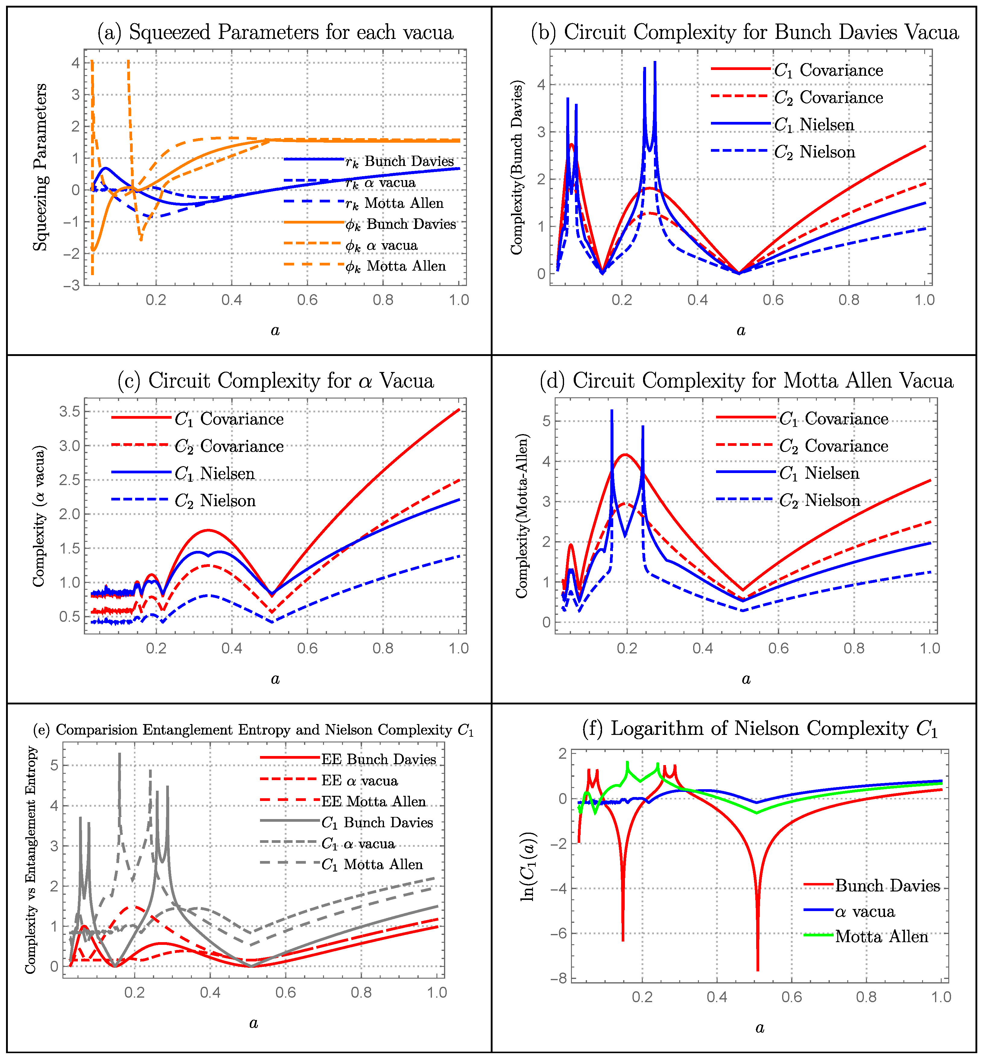
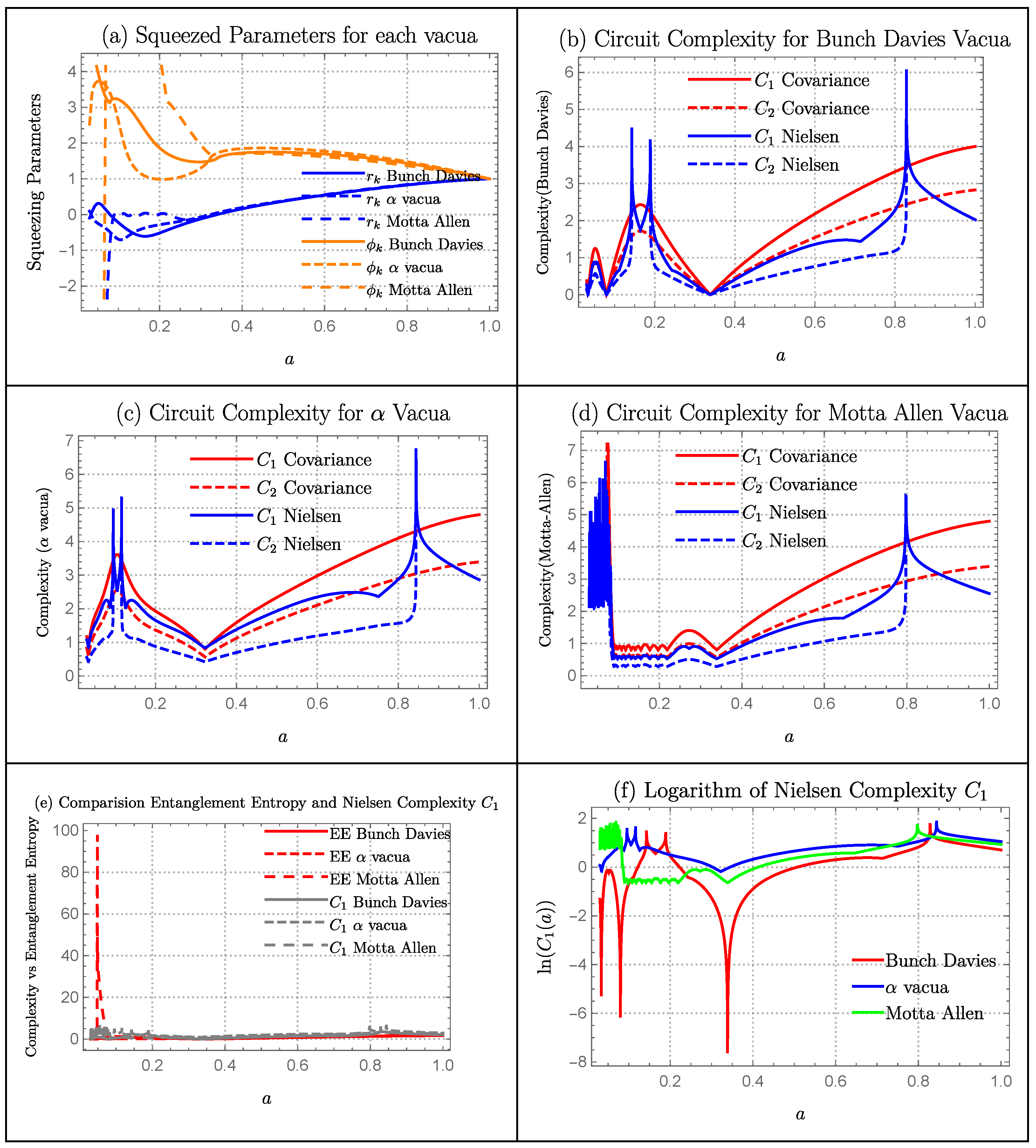
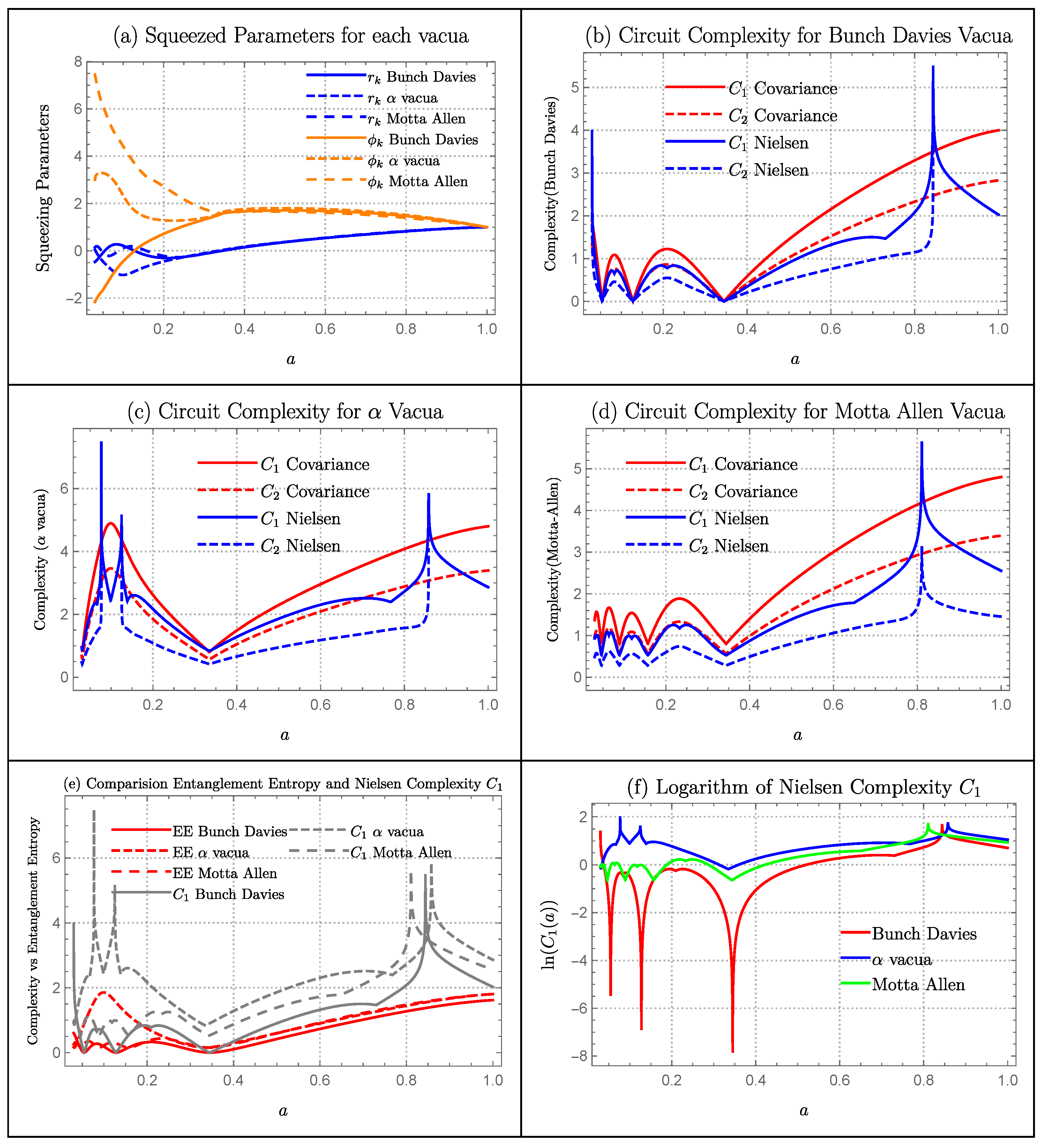
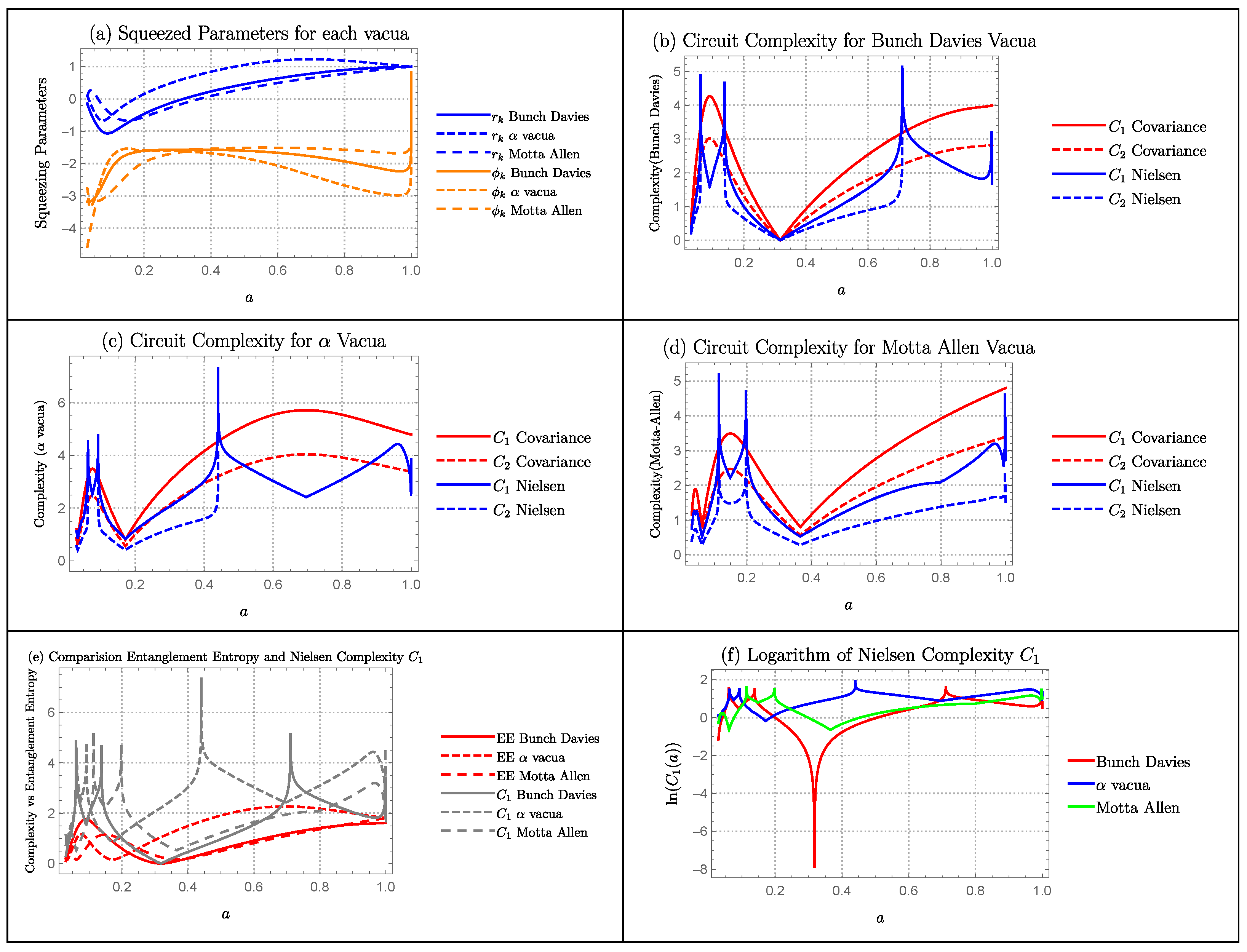
Contraction Bounce Model: In Figure 6a, we have plotted squeezing parameters $r_k$ and ${\varphi }_k$ for each vacua using the parameters $k=0.1,\alpha =0.2$ and $\gamma =0.4$. The growth of $r_k$ is very small for all vacua and they merge at each other. The evolution of ${\varphi }_k$ is different to Motta-Allen vacua than $\alpha$ and Bunch-Davies Vacua.

2.

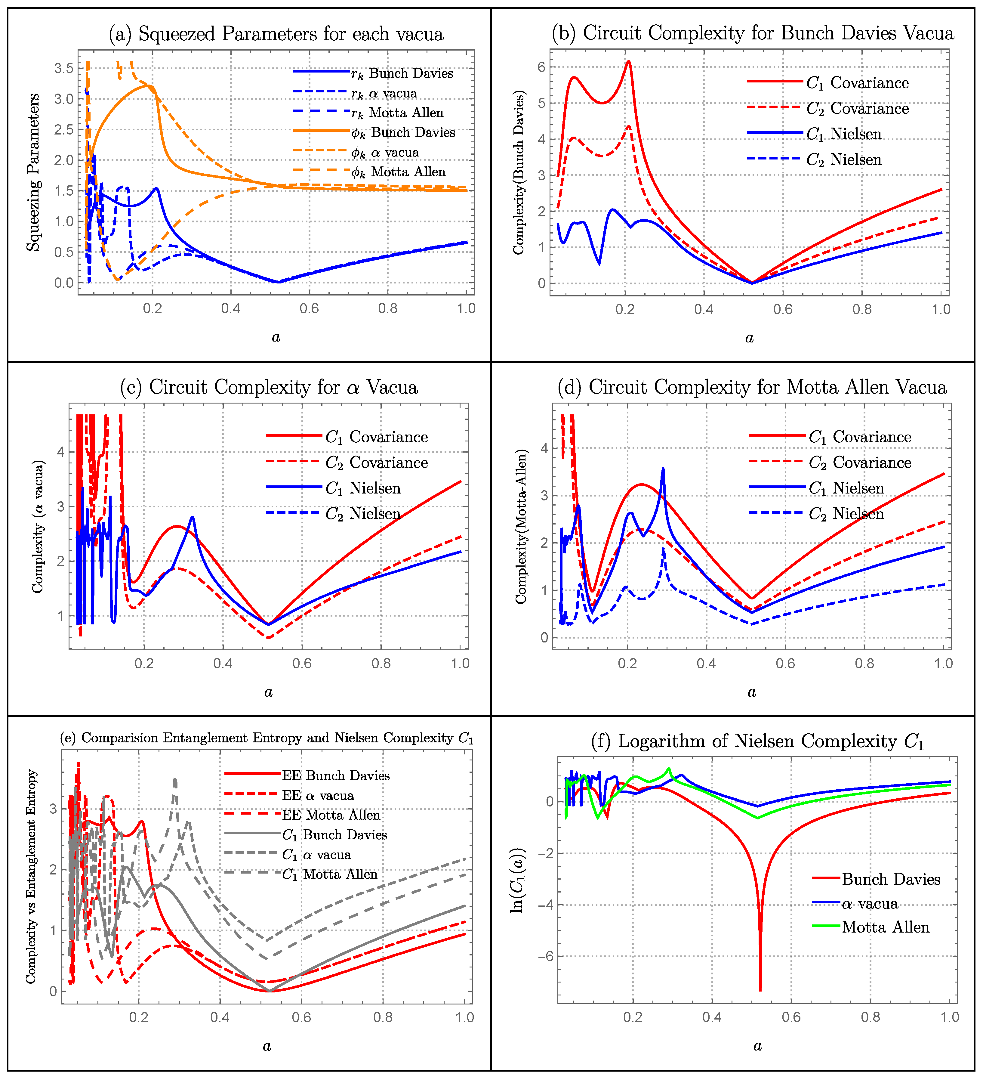
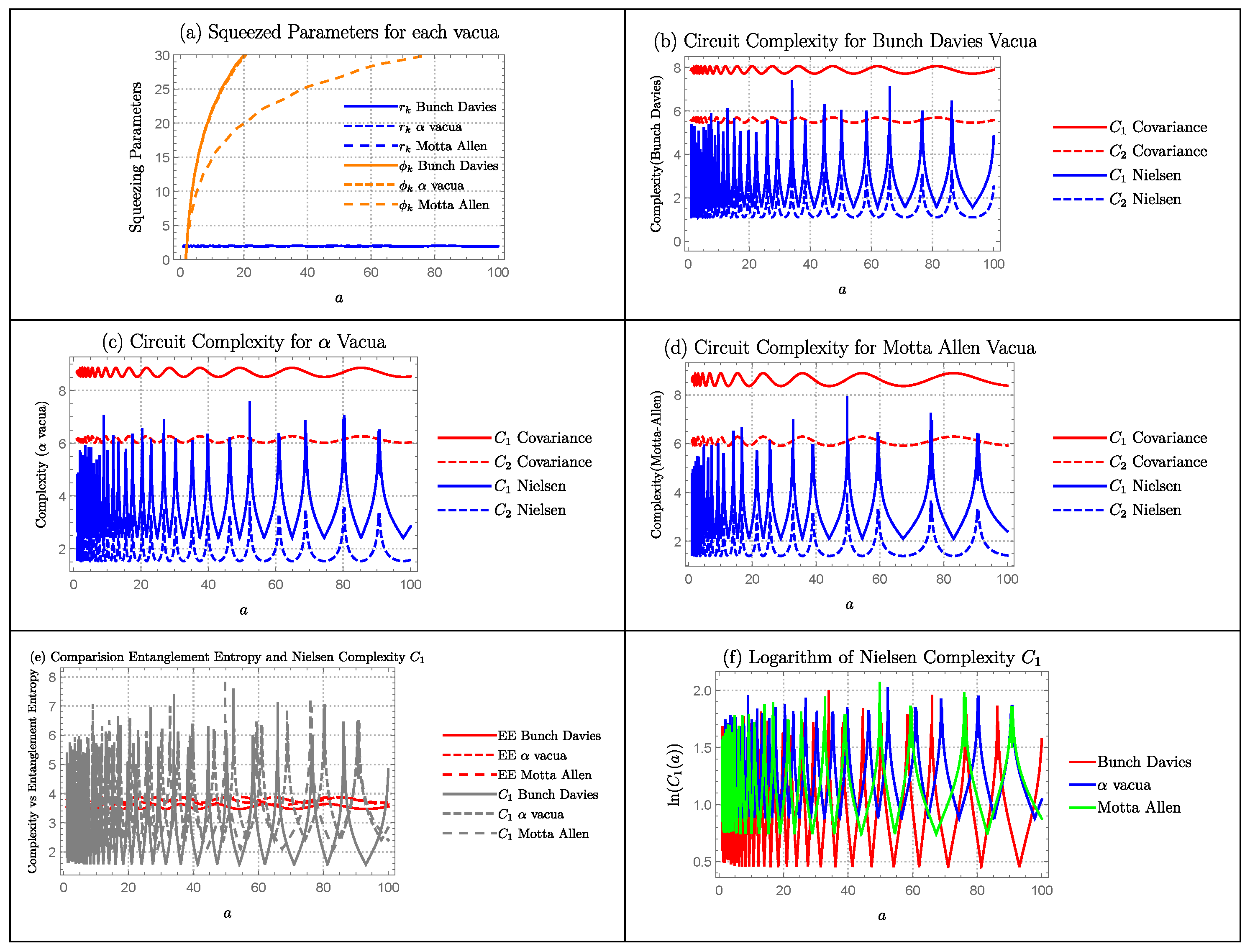
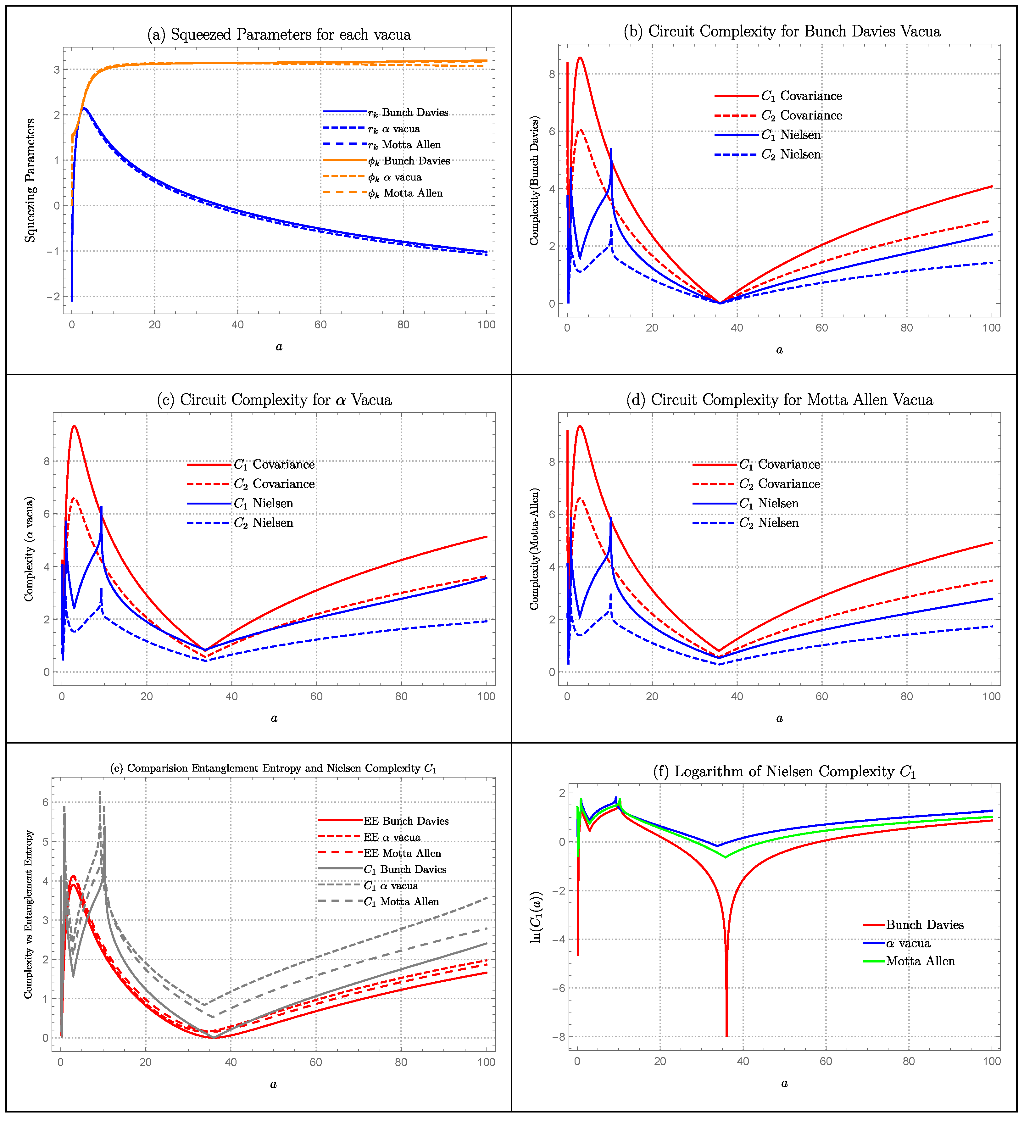
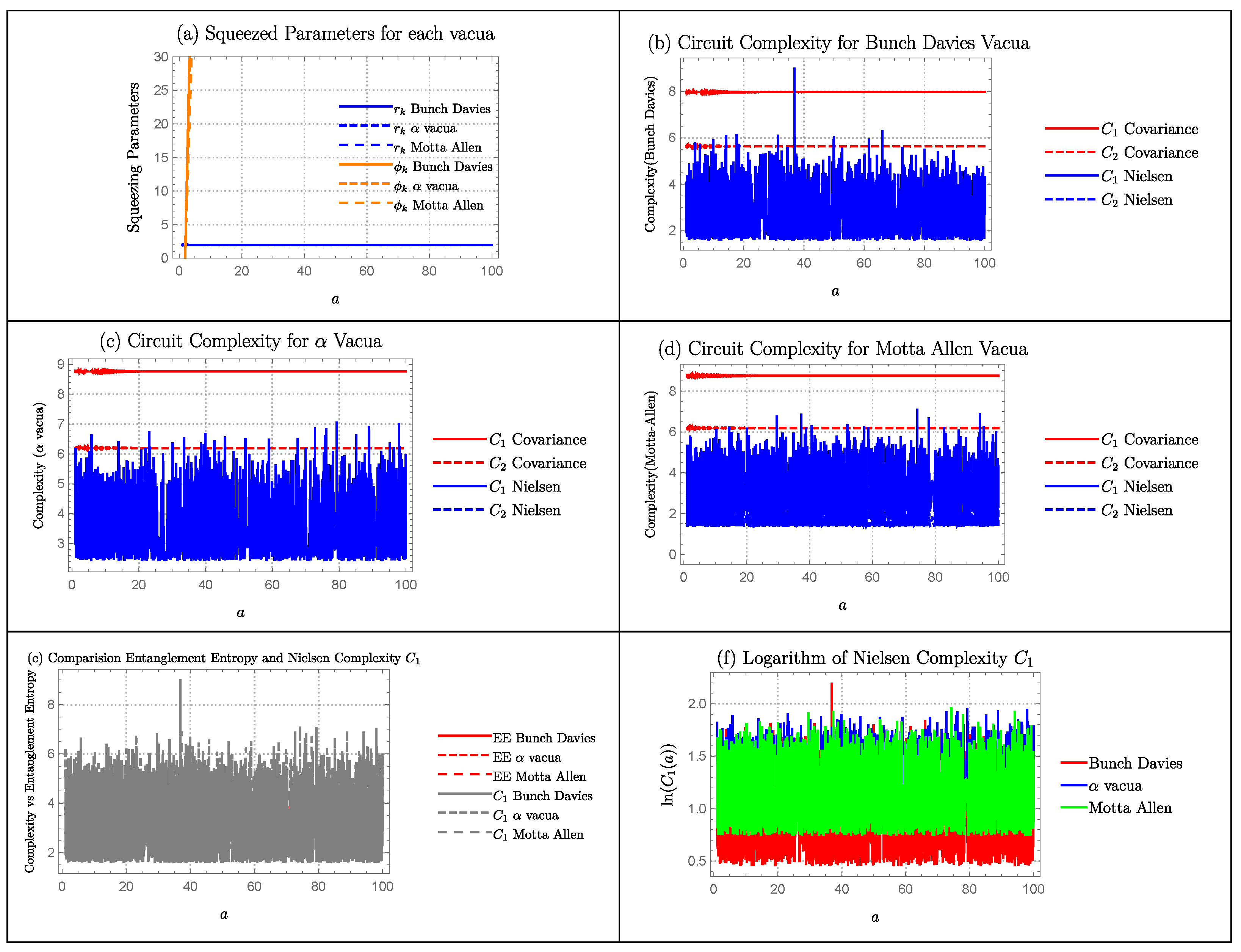
Matter Bounce Model: In Figure 7a, we have plotted squeezing parameters $r_k$ and ${\varphi }_k$ for each vacua using the parameters $k=0.1,\alpha =0.2$ and $\gamma =0.4$. For all three vacua, $r_k$ grows at the early values of scale factor a, and then keeps dropping. While for all three vacua, ${\varphi }_k$ grows and then saturates.

3.

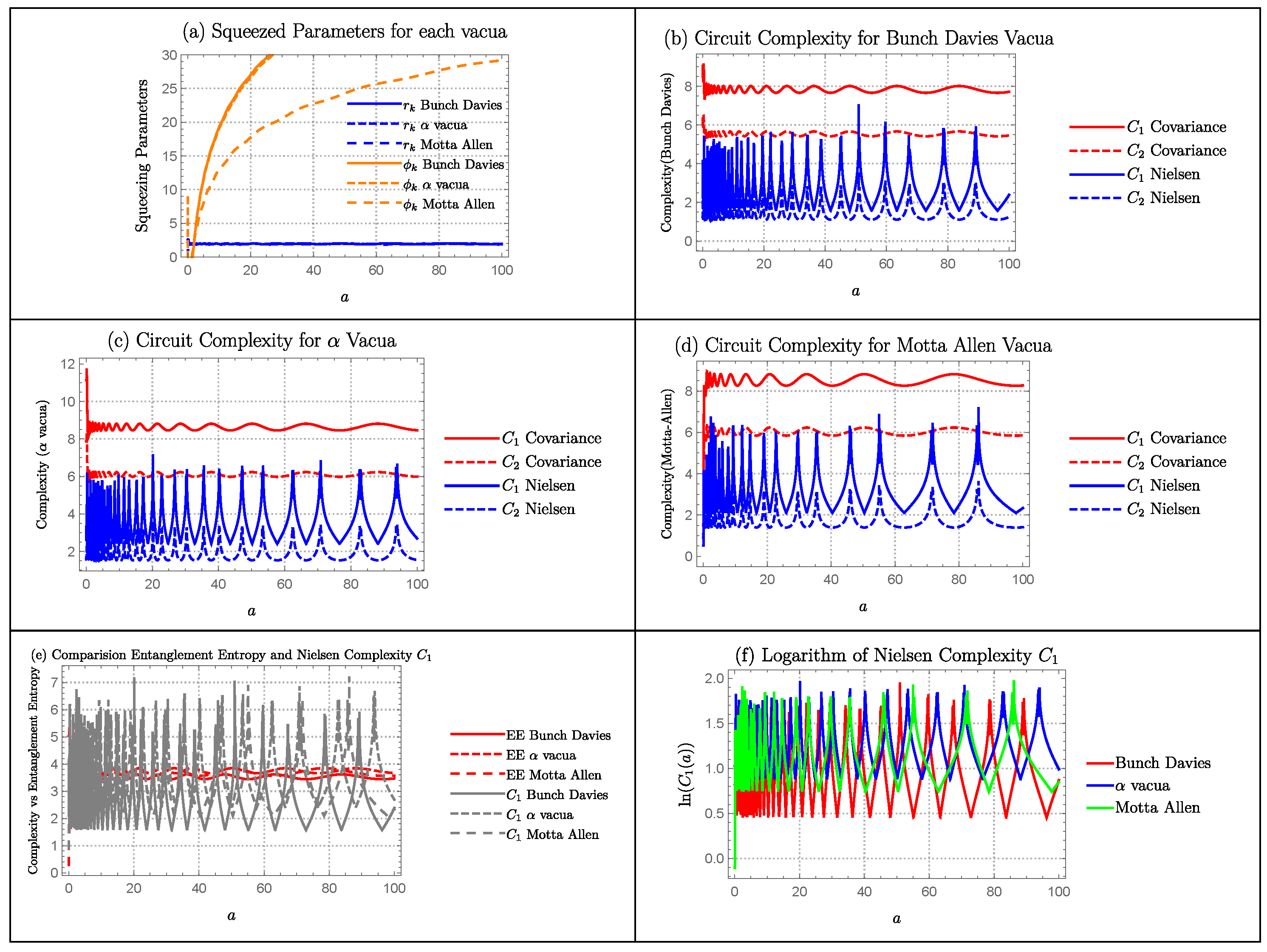
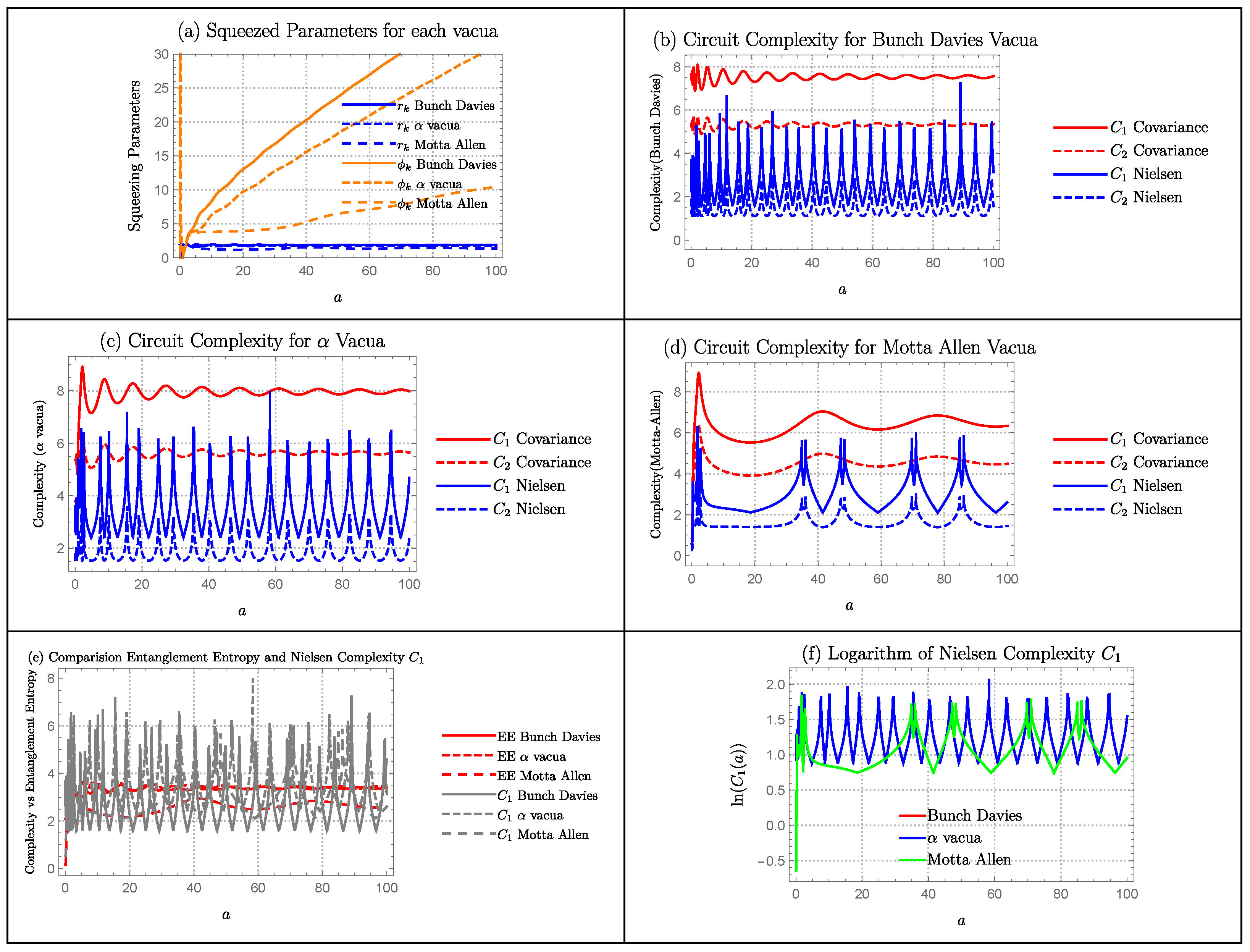
Sechyperbolic Bounce Model: In Figure 8a, we have plotted squeezing parameters $r_k$ and ${\varphi }_k$ for each vacua using the parameters $k=0.1,\alpha =0.2$ and $\gamma =0.4$. For all three vacua, $r_k$ keeps growing with respect to the scale factor a. While the behavior of ${\varphi }_k$ is different for each vacua at early a. Then, they starts to merge after some time.

4.

Cosinehyperbolic Bounce Model: In Figure 9a, we have plotted squeezing parameters $r_k$ and ${\varphi }_k$ for each vacua using the parameters $k=0.1,\alpha =0.2$ and $\gamma =0.4$. The growth of $r_k$ is very small for all vacua and they merge at each other. At early time, ${\varphi }_k$ starts to grow together with the evolution of ${\varphi }_k$ being different to Motta-Allen vacua than $\alpha$ and Bunch-Davies Vacua at later a.

5.

Sinehyperbolic Bounce Model: In Figure 10a, we have plotted squeezing parameters $r_k$ and ${\varphi }_k$ for each vacua using the parameters $k=0.1,\alpha =0.2$ and $\gamma =0.4$. The growth of $r_k$ is very small for all vacua and they merge at each other. At early time, ${\varphi }_k$ starts to grow together with the evolution of ${\varphi }_k$ being different to Motta-Allen vacua than $\alpha$ and Bunch-Davies Vacua at later a.

6.

Cosechyperbolic Bounce Model: In Figure 11a, we have plotted squeezing parameters $r_k$ and ${\varphi }_k$ for each vacua using the parameters $k=0.1,\alpha =0.2$ and $\gamma =0.4$. The growth of $r_k$ takes a dip around $a=0.15$ and then keeps a linear growth. This holds for all vacua. While value of ${\varphi }_k$ are different for each vacua until $a=0.3$, and then they merge. After that, they keep on dropping until it merge with $r_k$.

7.

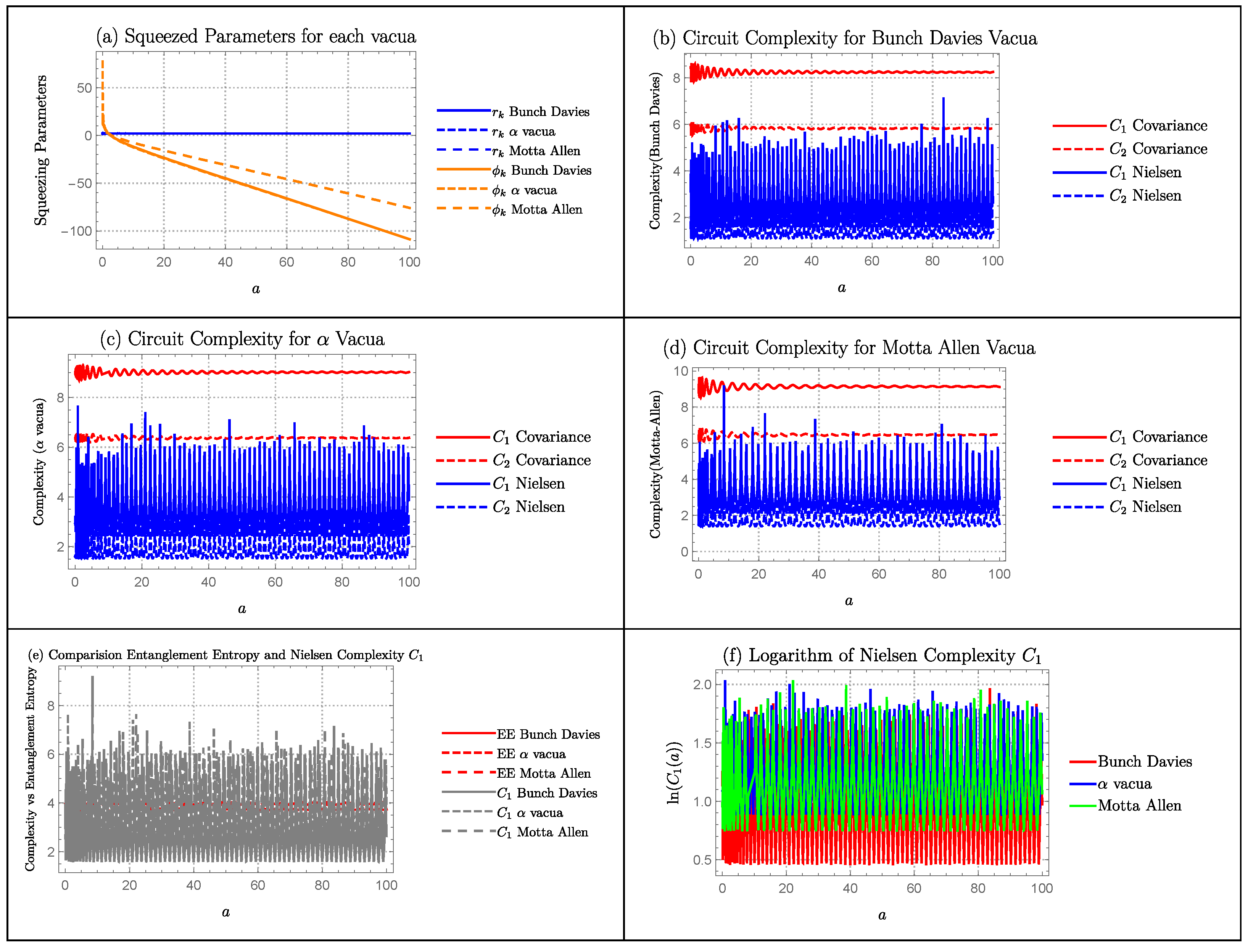
Exponential Bounce Model: In Figure 12a, we have plotted squeezing parameters $r_k$ and ${\varphi }_k$ for each vacua using the parameters $k=0.1,\alpha =0.2$ and $\gamma =0.4$. The value of $r_k$ is constant up to $a=0.35$, and then they starts to grow linearly. The value of ${\varphi }_k$ keeps dropping until it merges with $r_k$. This holds for all vacua.

8.

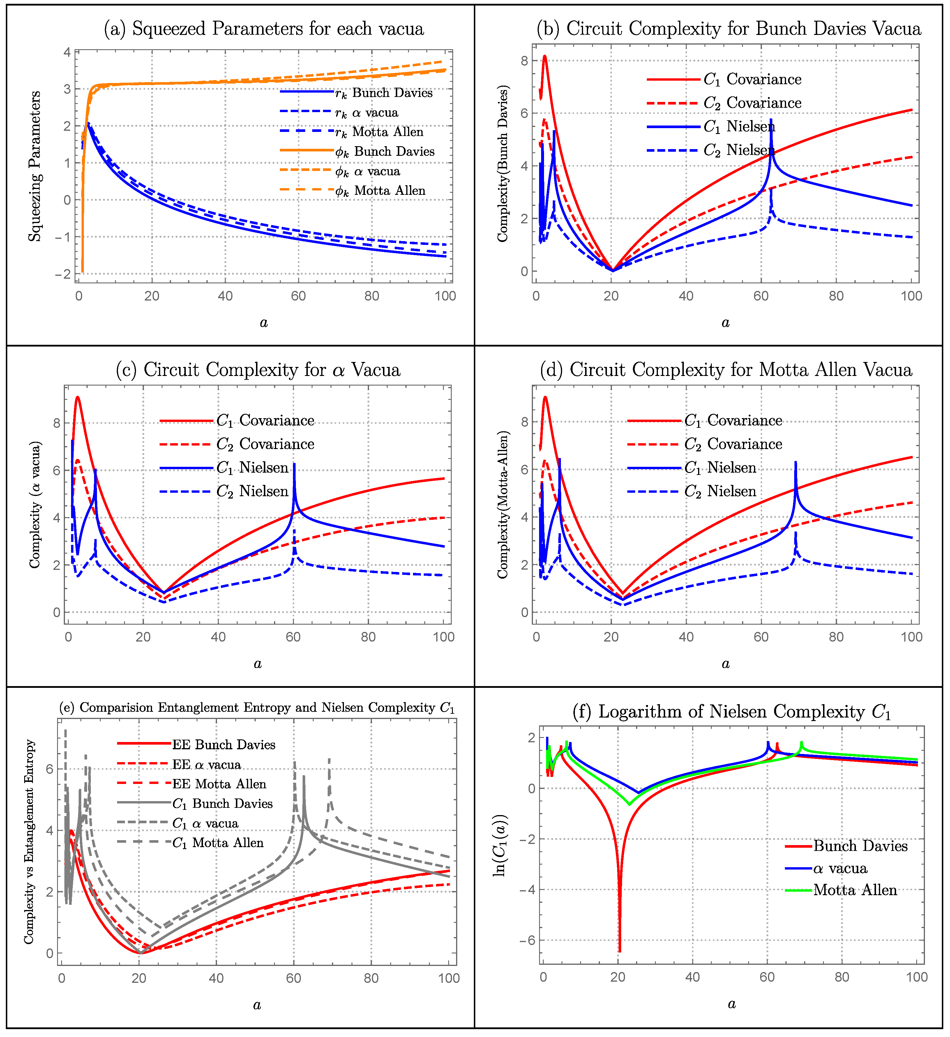
Power Law Bounce Model: In Figure 13a, we have plotted squeezing parameters $r_k$ and ${\varphi }_k$ for each vacua using the parameters $k=0.1,\alpha =0.2$ and $\gamma =0.4$. The value of $r_k$ takes a sharp growth and starts to drop. While ${\varphi }_k$ grows and then saturates.

9.

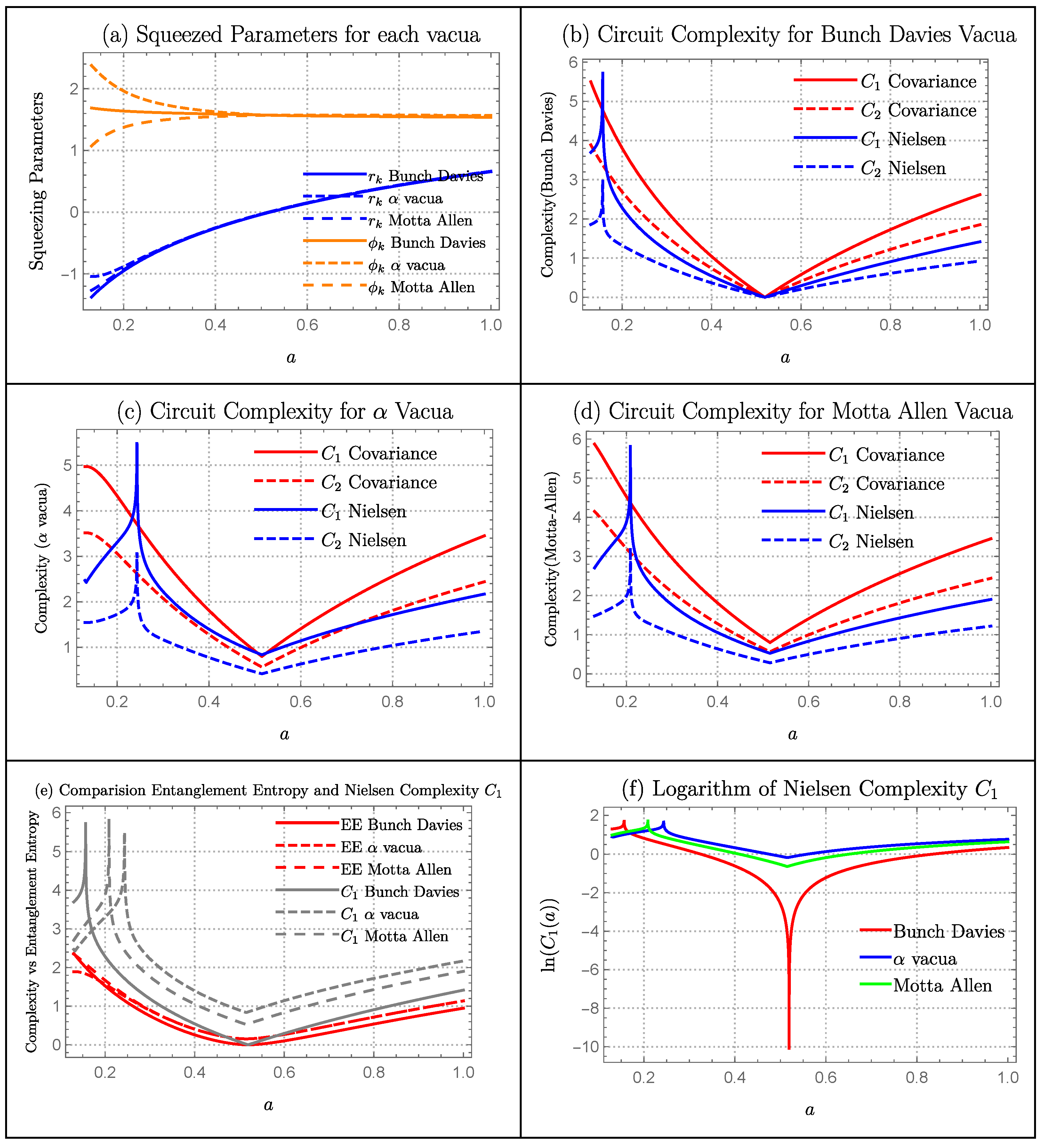
Polynomial Bounce Model: In Figure 14a, we have plotted squeezing parameters $r_k$ and ${\varphi }_k$ for each vacua using the parameters $k=0.1,\alpha =0.2$ and $\gamma =0.4$. The growth of $r_k$ is constant and almost same for each vacua. Bunch-Davies vauca has the largest growth of ${\varphi }_k$ followed by Alpha and then Motta-Allen vacua.

10.

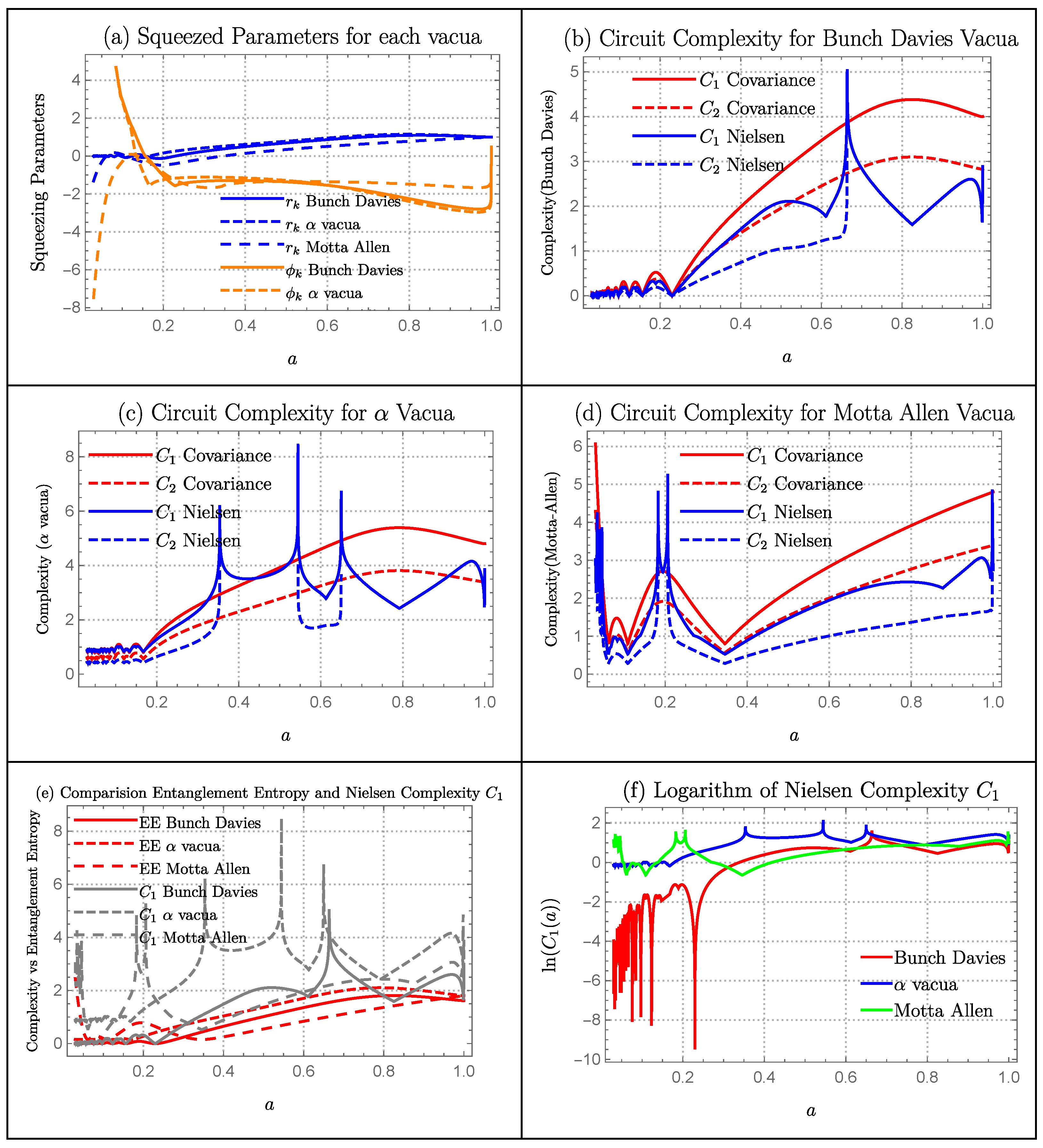
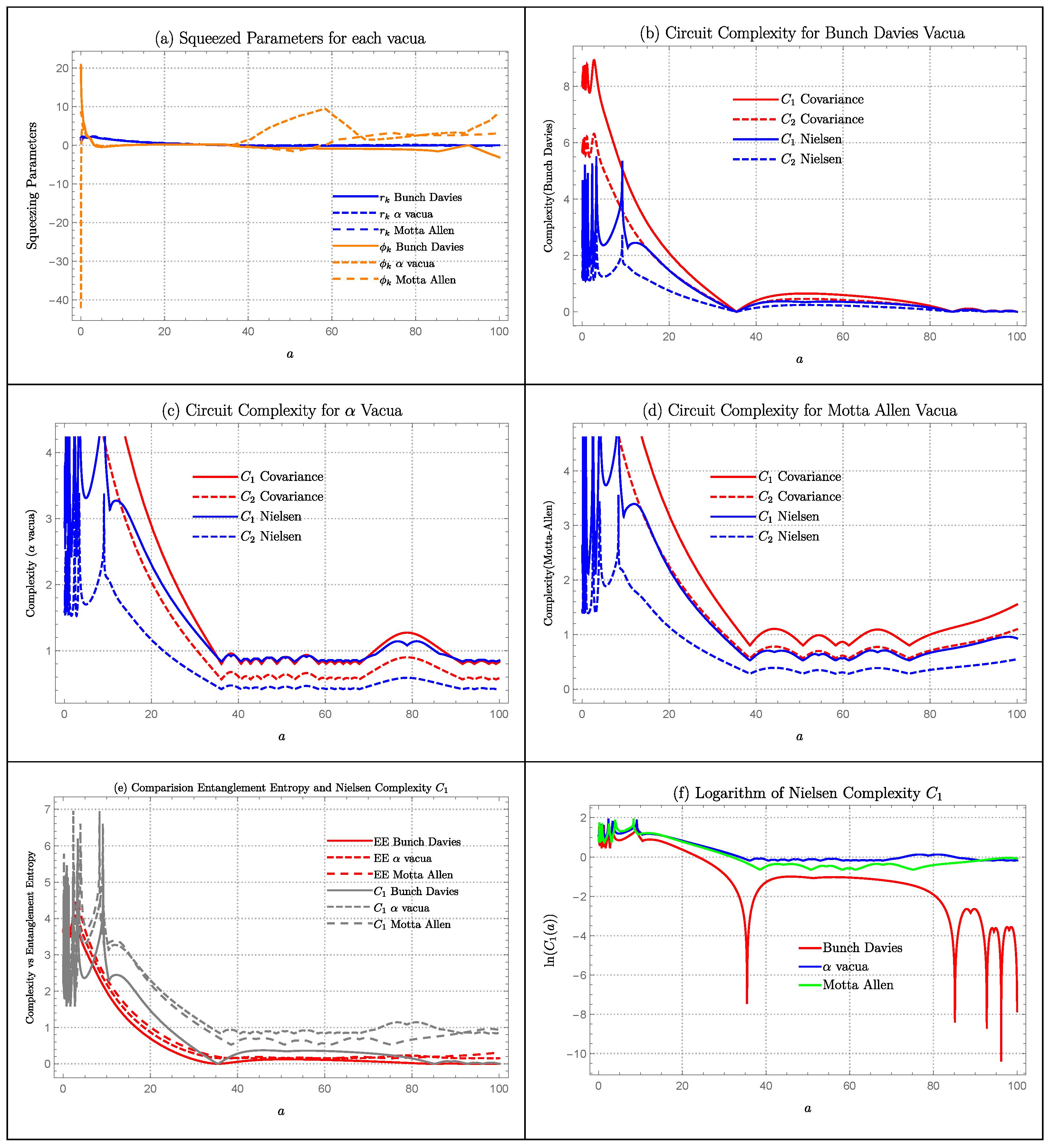
Expansion (Post-Bounce) Model: In Figure 15a, we have plotted squeezing parameters $r_k$ and ${\varphi }_k$ for each vacua using the parameters $k=0.1,\alpha =0.2$ and $\gamma =0.4$. The growth of $r_k$ is constant and almost same for each vacua. The growth of ${\varphi }_k$ is similar in the beginning for each vacua but they starts to diverge around $a=50$.

Complexity Measure

Figure 6, Figure 7, Figure 8, Figure 9, Figure 10, Figure 11, Figure 12, Figure 13, Figure 14 and Figure 15, in sub figure b–d, we have plotted the circuit complexity measures for Bunch-Davies Vacua, $\alpha$ Vacua and Motta-Allen Vacua respectively using both Covariance as well as Nielsen Approach using calculations from Section 4. Before discussing each case individually, let us discuss the overall features of these complexity measures. Covariance measure of complexity has similar pattern to the growth of squeezing parameter $r_k$. However, Nielsen’s complexity measure has more details on it. This is reasonable as Nielsen’s complexity measure is sensitive to both $r_k$ and ${\varphi }_k$.

1.

Contraction Bounce Model: Circuit complexity plots for each vacua is identical in overall pattern except for the magnitude. Overall, Motta-Allen Vacua has the largest magnitude with Bunch-Davies being lowest which is due to Motta-Allen Vacua having largest number of external parameters. Covariance measure of complexity is similar to the growth of the squeezing parameter $r_k$ with increase in magnitude. However, Nielsen’s measure is telling a different story. Nielsen’s measure of complexity is highly oscillatory for each vacua and for both cost function $C_1$ and $C_2$.

2.

Matter Bounce Model: Circuit complexity plots for each vacua is identical in overall pattern except for the magnitude. The plot for the covariance measure of complexity is smooth with a growth at early times and then taking a dip around $a=20$. After the dip, both $C_1$ and $C_2$ growing linearly. Nielsen measure of complexity has similar pattern but with more details on it. Around $a=60$, we can observe a pick in both $C_1$ and $C_2$. Even in early values of a, we can observe some oscillatory behaviour.

3.

Sechyperbolic Bounce Model: Interestingly, we can observe different behaviour in evolution of complexity for each vacua. For Bunch-Davies case, both $C_1$ and $C_2$ Covariance’s complexity is oscillatory before $a=0.2$, and then they keep growing with $C_2$ being bounded by $C_1$. While this pattern is visible for Nielsen’s approach too, there is a oscillatory around $a=0.65$. For $\alpha$ vacua, more such peaks are visible in Nielsen’s measure of complexity. In Motta-Allen Vacua, both covariance and Nielsen’s measure of complexity is oscillatory before $a=0.35$ after which they starts to take a smooth rise.

4.

Cosinehyperbolic Bounce Model: Circuit complexity plots for each vacua is identical in overall pattern except for the magnitude. Overall, Motta-Allen Vacua has the largest magnitude with Bunch davies being lowest which is due to Motta-Allen Vacua having largest number of external parameters. Covariance measure of complexity is similar to the growth of the squeezing parameter $r_k$ with increase in magnitude. However, Nielsen’s measure is telling a different story. Nielsen’s measure of complexity is highly oscillatory for each vacua and for both cost function $C_1$ and $C_2$. In all cases, $C_2$ is being bounded by $C_1$.

5.

Sinehyperbolic Bounce Model: Circuit complexity plots for each vacua is identical in overall pattern except for the magnitude. Overall, Motta-Allen Vacua has the largest magnitude with Bunch davies being lowest which is due to Motta-Allen Vacua having largest number of external parameters. Covariance measure of complexity is similar to the growth of the squeezing parameter $r_k$ with increase in magnitude. However, Nielsen’s measure is telling a different story. Nielsen’s measure of complexity is highly oscillatory for each vacua and for both cost function $C_1$ and $C_2$. In all cases, $C_2$ is being bounded by $C_1$.

6.

Cosechyperbolic Bounce Model: Interestingly, we can observe different behavior in evolution of complexity for each vacua. For Bunch-Davies case, both $C_1$ and $C_2$ Covariance’s complexity is oscillatory before $a=0.35$, and then they keep growing with $C_2$ being bounded by $C_1$. While this pattern is visible for Nielsen’s approach too, there is a oscillatory peak around $a=0.8$. Before $a=0.35$, the complexity measure is oscillatory just like for Bunch- Davies case but with more sharp peaks visible. In all cases, $C_2$ is being bounded by $C_1$.

7.

Exponential Bounce Model: The overall pattern of complexity measure is identical for each vacua expect for the change in magnitude. Covariance measure of complexity is similar to the growth of $r_k$ with $C_2$ being bounded by $C_1$. Nielsen’s measure of complexity is very oscillatory before $a=0.5$ after which it takes a growth and saturates.

8.

Power Law Bounce Model: The overall pattern of complexity measure is identical for each vacua expect for the change in magnitude. Covariance measure of complexity takes a sharp growth and takes a dip until $a=36$ and then keep a linear growth with $C_2$ being bounded by $C_1$. While this is also true for Nielsen’s measure, there are some peaks visible around $a=10$.

9.

Polynomial Bounce Model: Circuit complexity plots patter for Bunch-Davies and $\alpha$ vacua is identical in overall pattern except for the magnitude. For both vacua, covariance measure has the growth pattern similar to the squeezing parameter $r_k$. However, Nielsen’s measure of complexity is very oscillatory. For the case of Motta-Allen vacua, there are more gaps in the oscillatory peaks.

10.

Expansion (Post-Bounce) Model: For each vacua, circuit complexity drops until $a=35$ and then saturates around that point. In all vacua, Nielsen’s measure of complexity is quite chaotic and oscillatory before $a=10$. For $\alpha$ and Motta-Allen vacua, there are also more oscillatory bumps visible after the point $a=35$.

Comparison of Entanglement Entropy with Complexity

Entanglement entropy is a very popular probe to study the dynamics of quantum systems. We would like to see if circuit complexity can also be a similar candidate. In sub figure e, we have plotted a comparison of Nielsen’s circuit complexity $C_1$ and entanglement entropy. We have chosen Nielsen’s measure of complexity because, both Covariance complexity and entanglement entropy are independent of squeezing angle and depends linearly on squeezing parameter $r_k$. So, the pattern obtained from covariance measure of complexity will be similar as to entanglement entropy except that both complexity measure $C_1$ and $C_2$ is greater than entanglement entropy. However with Nielsen’s measure of complexity, we can obtain more interesting details of the system.

1.

Contraction Bounce Model: Complexity is highly oscillatory compared to the entanglement entropy.

2.

Matter Bounce Model: Both entanglement entropy and complexity measure has similar growth pattern. However, complexity measure has more peaks visible around $a=60$.

3.

Sechyperbolic Bounce Model: Again complexity measure has more oscillatory peaks compared to the entanglement entropy. This allows us to understand the system in more detail.

4.

Cosinehyperbolic Bounce Model: Complexity is highly oscillatory compared to the entanglement entropy.

5.

Sinehyperbolic Bounce Model: Complexity is highly oscillatory compared to the entanglement entropy.

6.

Cosechyperbolic Bounce Model: Both entanglement entropy and complexity has similar growth pattern but entanglement entropy has a very huge peak at early values of a.

7.

Exponential Bounce Model: Nielsen’s measure of complexity is very oscillatory before $a=0.5$ after which it takes a growth and saturates while entanglement entropy is not. But, entanglement entropy also takes a growth and saturates just like complexity measure.

8.

Power Law Bounce Model: Both complexity and entanglement entropy has a similar growth pattern, but there are some peaks visible around $a=10$ for the case of complexity measure.

9.

Polynomial Bounce Model: Complexity is highly oscillatory compared to the entanglement entropy.

10.

Expansion (Post-Bounce) Model: Nielsen’s measure of complexity is quite chaotic and oscillatory before $a=10$ but the overall pattern is similar to of entanglement entropy.

Quantum Lyapunov Exponent

Circuit complexity has also been proposed as a tool to measure quantum chaos. In particular, low growth of complexity indicates less chaotic system while higher growth of complexity indicates highly chaotic system. So, slope of the complexity could be a measure of quantum chaos. As a crude approximation, we will call the Lyapunov exponent ${\lambda }_i$ to be:

$${\lambda }_i=\frac{\ln C_i\left(\mathrm{point}\mathrm{of}\mathrm{saturation}\right)-\ln C_i\left(\mathrm{point}\mathrm{of}\mathrm{rise}\right)}{a\left(\mathrm{point}\mathrm{of}\mathrm{saturation}\right)-a\left(\mathrm{point}\mathrm{of}\mathrm{rise}\right)}$$

(287)

where i indicates the choice of vacua. For simplicity, we will restrict to Nielsen complexity $C_1$ and we will obtain Lyapunov exponent ${\lambda }_i$.

1.

Contraction Bounce Model: The log. complexity plot is too oscillatory to get the chaotic measure.

2.

Matter Bounce Model:

$$\begin{array}{cc}\hfill {\lambda }_{Motta-Allen}& =0.008\hfill \\ \hfill {\lambda }_{\alpha }& =0.007\hfill \\ \hfill {\lambda }_{Bunch-Davies}& =0.008\hfill \end{array}$$

(288)

All three vacua has similar lyapunov exponent, so they have similar chaotic properties.

3.

Sechyperbolic Bounce Model:

$$\begin{array}{cc}\hfill {\lambda }_{Motta-Allen}& =1\hfill \\ \hfill {\lambda }_{\alpha }& =0.01\hfill \\ \hfill {\lambda }_{Bunch-Davies}& =0.16\hfill \end{array}$$

(289)

Motta-Allen Vacua has the largest lyapunov exponent, so it is the most chaotic cosmological model followed by Bunch-Davies and $\alpha$ vacua.

4.

Cosinehyperbolic Bounce Model: The log. complexity plot is too oscillatory to get the chaotic measure.

5.

Sinehyperbolic Bounce Model: The log. complexity plot is too oscillatory to get the chaotic measure.

6.

Cosechyperbolic Bounce Model:

$$\begin{array}{cc}\hfill {\lambda }_{Motta-Allen}& =1.25\hfill \\ \hfill {\lambda }_{\alpha }& =0.41\hfill \\ \hfill {\lambda }_{Bunch-Davies}& =2.91\hfill \end{array}$$

(290)

Bunch-Davies Vacua has the largest Lyapunov exponent, so it is the most chaotic cosmological model followed by Motta-Allen and $\alpha$ vacua.

7.

Exponential Bounce Model:

$$\begin{array}{cc}\hfill {\lambda }_{Motta-Allen}& =0.83\hfill \\ \hfill {\lambda }_{\alpha }& =0.75\hfill \\ \hfill {\lambda }_{Bunch-Davies}& =0.75\hfill \end{array}$$

(291)

All three vacua has similar Lyapunov exponent, so they have similar chaotic properties.

8.

Power Law Bounce Model:

$$\begin{array}{cc}\hfill {\lambda }_{Motta-Allen}& =0.02\hfill \\ \hfill {\lambda }_{\alpha }& =0.01\hfill \\ \hfill {\lambda }_{Bunch-Davies}& =0.03\hfill \end{array}$$

(292)

All three vacua has similar Lyapunov exponent, so they have similar chaotic properties.

9.

Polynomial Bounce Model: The log. complexity plot is too oscillatory to get the chaotic measure.

10.

Expansion (Post-Bounce) Model: There is no growth or saturation point of complexity, so we will not be able to get the chaotic measure.

6.7. Cyclic Models

In Figure 16 and Figure 17, we have numerically plotted the squeezing parameters, derived circuit complexity measures for Bunch-Davies Vacua, $\alpha$ Vacua and Motta-Allen Vacua, comparison of entanglement entropy with circuit complexity measure and quantum chaos for Matter cyclic and Radiation cyclic model on super-horizon scales for the parameters $k=0.1,\alpha =0.2$ and $\gamma =0.4$. We have set $r_k(a=1)=1,{\varphi }_k(a=1)=1$ as our initial conditions. The extra parameters we have selected for each bouncing model will be highlighted under it’s own headings.

Squeezing Parameters

For each figures from Figure 16 and Figure 17, in sub figure a, we have plotted squeezing parameters $r_k$ and ${\varphi }_K$ for each vacua using the parameters that will be given below. Since all measures of interest such as Complexity, Entropy and Chaos are dependent on these parameters, it is crucial to understand their behavior.

1.

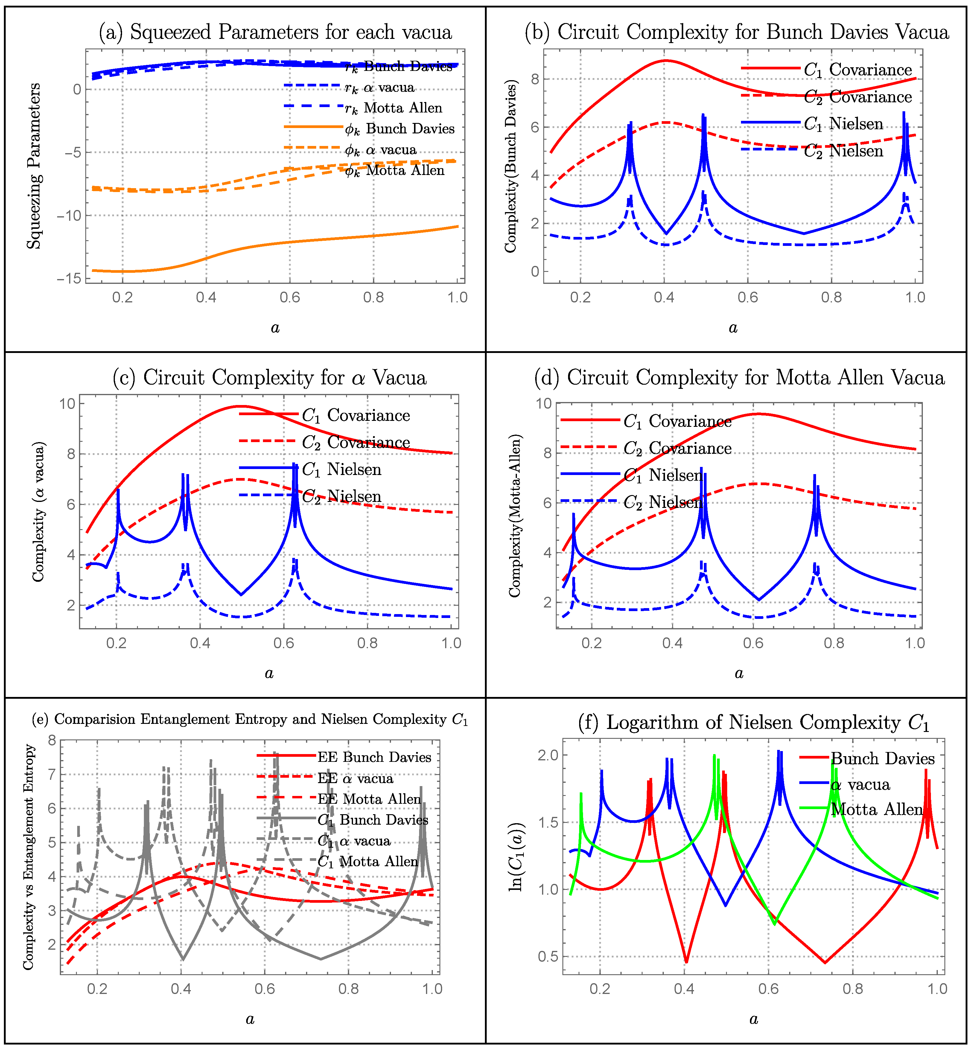
Matter cyclic model: In Figure 16a, we have plotted squeezing parameters $r_k$ and ${\varphi }_k$ for each vacua using the parameters $k=0.1,\alpha =0.2$ and $\gamma =0.4$. Before $a=0.2$, $r_k$ is different for each vacua. However, after that point, they merge and starts to grow linearly. While before $a=0.3$, ${\varphi }_k$ is different for each vacua, after that point they merge and saturates.

2.

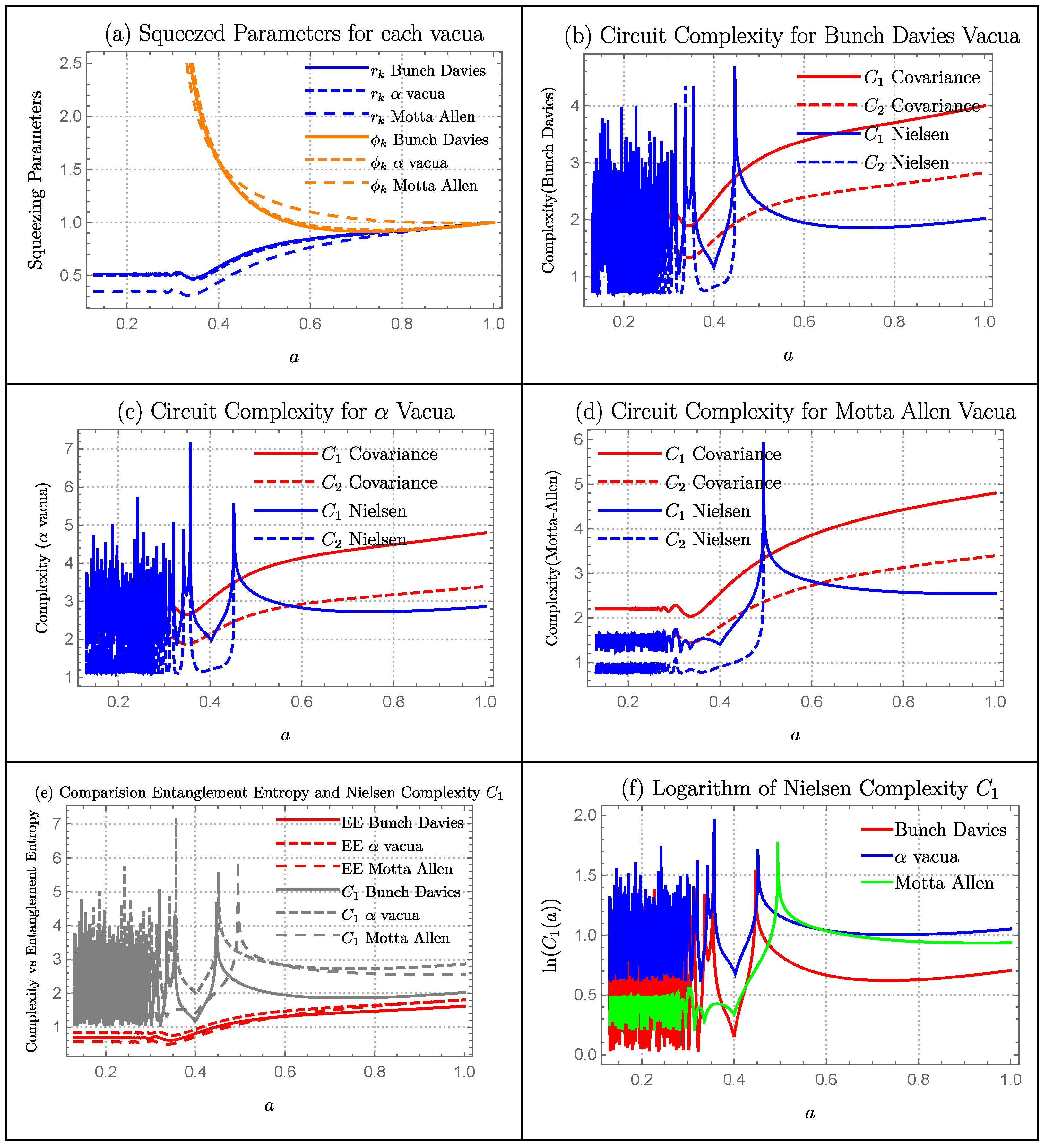
Radiation cyclic model: In Figure 17a, we have plotted squeezing parameters $r_k$ and ${\varphi }_k$ for each vacua using the parameters $k=0.1,\alpha =0.2$ and $\gamma =0.4$. The value of $r_k$ grows for each vacua but with a different magnitude. $\alpha$ vacua has the largest magnitude while Bunch-Davies and Motta-Allen have comparable values of $r_k$. At early values of a, ${\varphi }_k$ grows for each vacua and saturates. However at around $a=1$, all three vacua merges and takes a sharp growth.

Complexity Measure

For each figures from Figure 16 and Figure 17, in sub figure b–d, we have plotted the circuit complexity measures for Bunch-Davies Vacua, $\alpha$ Vacua and Motta-Allen Vacua respectively using both Covariance as well as Nielsen Approach using calculations from Section 4. Before discussing each case individually, let us discuss the overall features of these complexity measures. Covariance measure of complexity has similar pattern to the growth of squeezing parameter $r_k$. However, Nielsen’s complexity measure has more details on it. This is reasonable as Nielsen’s complexity measure is sensitive to both $r_k$ and ${\varphi }_k$.

1.

Matter cyclic model: For Bunch-Davies and Motta-Allen Vacua, covariance measure of complexity has a similar pattern but with different magnitude. Until $a=0.35$, it is oscillatory in nature with small magnitude. After which, it takes a linear growth. For $\alpha$ vacua, complexity grows at early values of a, then take a dip at $a=0.35$, and then grows linearly. Nielsen’s measure of complexity also has a similar pattern as covariance but has a peak around $a=0.8$.

2.

Radiation cyclic model: Covariance measure of complexity has the similar pattern for all three vacua. It grows at early values of a, then take a dip and then grows linearly. The point of dip is different for each vacua. However, Nielsen’s measure of complexity has more details coming from peaks at different values of a.

Comparison of Entanglement Entropy with Complexity

Entanglement entropy is a very popular probe to study the dynamics of quantum systems. We would like to see if circuit complexity can also be a similar candidate. In Figure 16e and Figure 17e, we have plotted a comparison of Nielsen’s circuit complexity $C_1$ and entanglement entropy. We have chosen Nielsen’s measure of complexity because, both Covariance complexity and entanglement entropy are independent of squeezing angle and depends linearly on squeezing parameter $r_k$. So, the pattern obtained from covariance measure of complexity will be similar as to entanglement entropy except that both complexity measure $C_1$ and $C_2$ is greater than entanglement entropy. However with Nielsen’s measure of complexity, we can obtain more interesting details of the system.

1.

Matter Cyclic Model: Both entanglement entropy and complexity measure has similar growth pattern. However, complexity measure has more peaks visible around $a=0.8$.

2.

Radiation Cyclic Model: Both entanglement entropy and complexity measure has similar growth pattern. However, complexity measure has more peaks. This shows that complexity measure is able to carry more details regarding the system compared to matter cyclic model.

Quantum Lyapunov Exponent

Circuit complexity has also been proposed as a tool to measure quantum chaos. In particular, low growth of complexity indicates less chaotic system while higher growth of complexity indicates highly chaotic system. So, slope of the complexity could be a measure of quantum chaos. As a crude approximation, we will call the lyapunov exponent ${\lambda }_i$ to be:

$${\lambda }_i=\frac{\ln C_i\left(\mathrm{point}\mathrm{of}\mathrm{saturation}\right)-\ln C_i\left(\mathrm{point}\mathrm{of}\mathrm{rise}\right)}{a\left(\mathrm{point}\mathrm{of}\mathrm{saturation}\right)-a\left(\mathrm{point}\mathrm{of}\mathrm{rise}\right)}$$

(293)

where i indicates the choice of vacua. For simplicity, we will restrict to Nielsen complexity $C_1$ and we will obtain lyapunov exponent ${\lambda }_i$.

1.

Matter Cyclic Model:

$$\begin{array}{cc}\hfill {\lambda }_{Motta-Allen}& =1.83\hfill \\ \hfill {\lambda }_{\alpha }& =1.33\hfill \\ \hfill {\lambda }_{Bunch-Davies}& =3.16\hfill \end{array}$$

(294)

Bunch-Davies Vacua has the largest lyapunov exponent, so it is the most chaotic cosmological model followed by Motta-Allen and $\alpha$ vacua.

2.

Radiation Cyclic Model:

$$\begin{array}{cc}\hfill {\lambda }_{Motta-Allen}& =2\hfill \\ \hfill {\lambda }_{\alpha }& =0.33\hfill \\ \hfill {\lambda }_{Bunch-Davies}& =2.5\hfill \end{array}$$

(295)

Bunch-Davies Vacua has the largest lyapunov exponent, so it is the most chaotic cosmological model followed by Motta-Allen and $\alpha$ vacua.

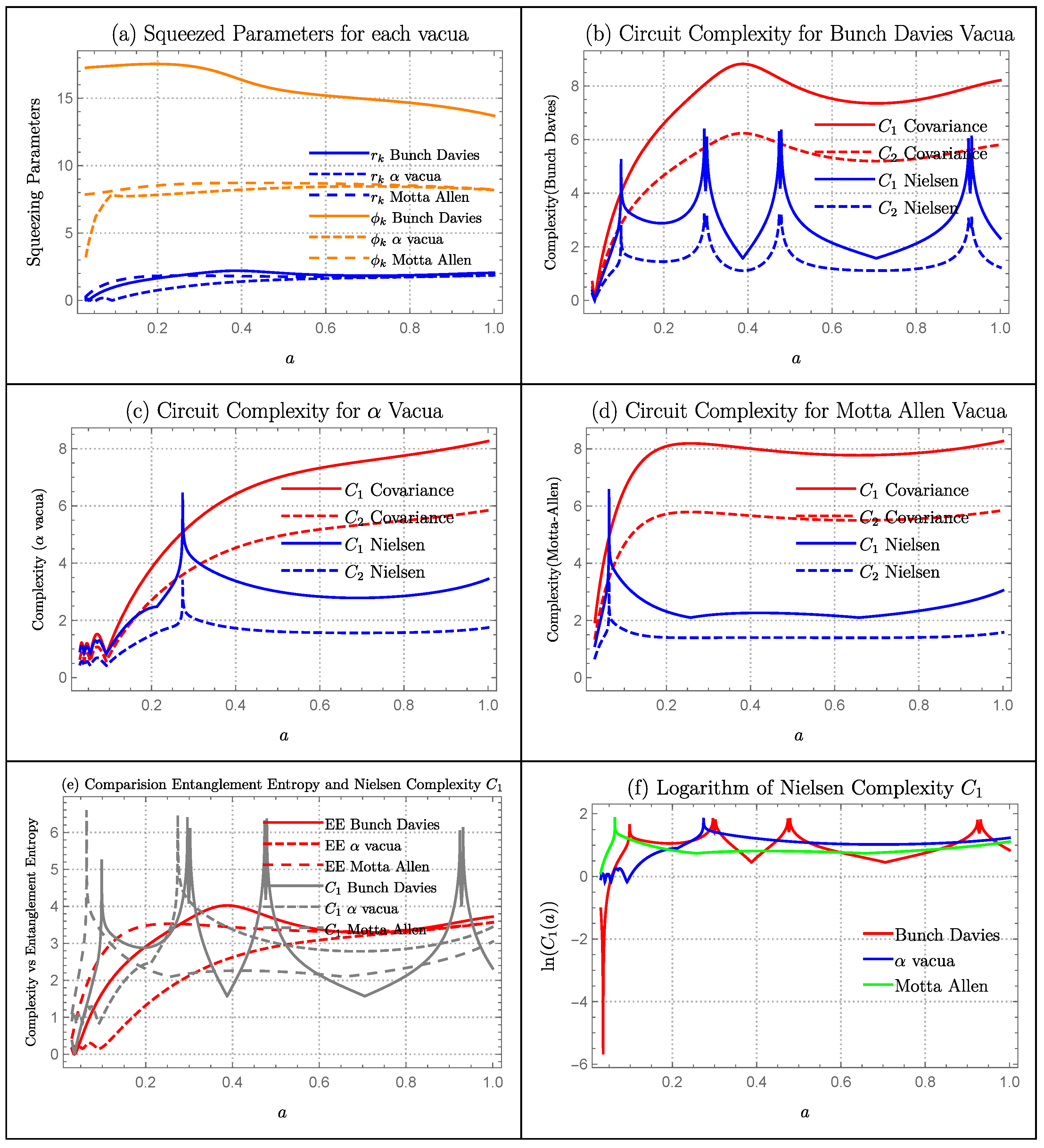
6.8. Black Hole Gas

In Figure 18, we have numerically plotted the squeezing parameters, derived circuit complexity measures for Bunch-Davies Vacua, $\alpha$ Vacua and Motta-Allen Vacua, comparison of entanglement entropy with circuit complexity measure and quantum chaos in de Sitter Model on super-horizon scales for the parameters $k=0.1$, $\alpha =0.2$ and $\gamma =0.4$. We have set $r_k(a=1)=1,{\varphi }_k(a=1)=1$ as our initial conditions.

Squeezing Parameters

In Figure 18a, we have plotted squeezing parameters $r_k$ and ${\varphi }_K$ for each vacua using the parameters listed above. $r_k$ takes a constant growth while ${\varphi }_k$ grows very quickly. Since both circuit complexity and entanglement entropy are strongly dependent on the values of these parameters, the behavior of these parameters are significant to understand the dynamics of the system.

Complexity Measure

In Figure 18b–d, we have plotted the circuit complexity measures for Bunch-Davies Vacua, $\alpha$ Vacua and Motta-Allen Vacua respectively using both Covariance as well as Nielsen Approach using calculations from Section 4. Nielsen’s measure of complexity is very oscillatory while Covariance measure grows similar to $r_k$ but with larger magnitude.

Comparison of Entanglement Entropy with Complexity

Entanglement entropy is a very popular probe to study the dynamics of quantum systems. We would like to see if circuit complexity can also be a similar candidate. In Figure 18e, we have plotted a comparison of Nielsen’s circuit complexity $C_1$ and entanglement entropy. We have chosen Nielsen’s measure of complexity because, both Covariance complexity and entanglement entropy are independent of squeezing angle and depends linearly on squeezing parameter $r_k$. So, the pattern obtained from covariance measure of complexity will be similar as to entanglement entropy except that both complexity measure $C_1$ and $C_2$ is greater than entanglement entropy. However with Nielsen’s measure of complexity, we can obtain more interesting details of the system such as the oscillatory behavior of complexity which is absent in entanglement entropy.

Quantum Lyapunov Exponent

Circuit complexity has also been proposed as a tool to measure quantum chaos. In particular, low growth of complexity indicates less chaotic system while higher growth of complexity indicates highly chaotic system. So, slope of the complexity could be a measure of quantum chaos. Because Nielsen’s measure of complexity is too oscillatory and doesn’t reach a saturation point, we will not be able to compute the lyapunov exponent term.

7. Conclusions

From our study we have the following final remarks:

• Compared to that calculated using the covariance matrix method, the circuit complexity computed using Nielsen’s wave function approach offers a much better understanding because it relies on the squeezing angle and the squeezing parameter and can therefore be linked to the entanglement entropy.
• We have computed the circuit complexity using both Nielsen’s wave function approach and Covariance matrix approach. From the study of both approaches to compute complexity in different cosmological models, it is clear that the overall pattern one obtain is similar in both cases. However, the circuit complexity computed from Nielsen’s wave function approach gives a much detailed understanding of the evolution of the system. The reason is that covariance measure of complexity is insensitive to the squeezing angle.
• The behaviour of the squeezing parameter is also different for each vacua: Bunch-Davies, $\alpha$ vacua and Motta-Allen Vacua. The reason for this is that dispersion relation for each vacua is different. So, while solving the set of differential equations, we will get different solutions for the squeezing parameter.
• We have computed the circuit complexity for all three vacua: Bunch-Davies, $\alpha$ vacua and Motta-Allen Vacua. Because the dispersion relation for each vacua is different, the solutions for the squeezing parameter is also different. This has the direct consequence in the properties of complexity measure. In addition, Motta-Allen and $\alpha$ vacua have more parameters than the simple Bunch-Davies vacua. This is also reflected in the complexity measure. Most of the times, Motta-Allen vacua has the largest complexity magnitude followed by $\alpha$ vacua and then Bunch-Davies vacua.
• The behavior of the entanglement entropy is also different for each vacua. Again, this is the result of having different set of solutions for the squeezing parameter. The values of entanglement entropy is bounded by the covariance measure of complexity $C_1$ and $C_2$. Entanglement entropy has the similar pattern as the covariance measure of complexity because both are independent of the squeezing angle ${\varphi }_k$. However, entanglement entropy has the different behaviour than the Nielsen’s measure of complexity. We are able to see more details in the complexity that is not visible in entanglement entropy growth. This shows that, complexity could also be a probe to detect important properties of a quantum system just like entanglement entropy. Since entanglement entropy is sometimes ridiculously difficult to compute, complexity could be a better alternative at those cases.
• The behaviour of circuit complexity is very dependent on the model and scale factor involved. For example: Nielsen’s measure of complexity is extremely oscillatory for models like Polynomial bounce and Sinehyperbolic bounce while very smooth for models like de-Sitter.

The future prospects of the work are:

• We have made qualitative comments on the relation between growth of complexity and quantum chaos. It would be interesting to see if it can be rigorously proven. One way could be to use the quantum speed limit properties to show the bound on complexity. Using Random Matrix theory, one can associate the bound on quantum speed limit to quantum chaos.
• For the framework of two-mode squeezed states, quantum complexity computed using Covariance matrix show similar feature that of entanglement entropy. It would be interesting to see if this holds true for other models.
• The relation between entanglement entropy and complexity can be studied in even more detail.
• In this paper, we have only studied the complexity measure for various cosmological models. It would be interesting to apply the lesson from these complexity plots to study the physical evolution of these models and observe to what extent it actually matches. Furthermore, concrete experimental prediction would be much desirable.

References

- Abbott, B.P.; Abbott, R.; Abbott, T.D.; Abernathy, M.R.; Acernese, F.; Ackley, K.; Cavalieri, R. Observation of Gravitational Waves from a Binary Black Hole Merger. Phys. Rev. Lett. 2016, 116, 061102. [Google Scholar] [CrossRef] [PubMed]
- Guzzetti, M.C.; Bartolo, N.; Liguori, M.; Matarrese, S. Gravitational waves from inflation. Riv. Nuovo Cim. 2016, 39, 399–495. [Google Scholar]
- Mather, J.C.; Cheng, E.S.; Eplee, R.E., Jr.; Isaacman, R.B.; Meyer, S.S.; Shafer, R.A.; Wilkinson, D.T. A Preliminary Measurement of the Cosmic Microwave Background Spectrum by the Cosmic Background Explorer (COBE) Satellite. Astrophys. J. 1990, 354, L37. [Google Scholar] [CrossRef]
- Akrami, Y.; Arroja, F.; Ashdown, M.; Aumont, J.; Baccigalupi, C.; Ballardini, M.; Savelainen, M. Planck 2018 results. X. Constraints on inflation. Astron. Astrophys. 2020, 641, A10. [Google Scholar]
- Aghanim, N.; Akrami, Y.; Ashdown, M.; Aumont, J.; Baccigalupi, C.; Ballardini, M.; Roudier, G. Planck 2018 results. VI. Cosmological parameters. Astron. Astrophys. 2020, 641, A6, Erratum: Astron. Astrophys. 2021, 652, C4. [Google Scholar]
- Baumann, D. Tasi Lectures on Inflation. arXiv 2012, arXiv:0907.5424. [Google Scholar]
- Baumann, D. Tasi lectures on primordial cosmology. arXiv 2018, arXiv:1807.03098. [Google Scholar]
- Mukhanov, V.; Winitzki, S. Introduction to Quantum Effects in Gravity; Cambridge University Press: Cambridge, UK, 2007; p. 6. [Google Scholar]
- Birrell, N.D.; Davies, P.C.W. Quantum Fields in Curved Space; Cambridge Monographs on Mathematical Physics; Cambridge University Press: Cambridge, UK, 1982. [Google Scholar]
- Grishchuk, L.P.; Sazhin, M.V. Squeezed quantum states of a harmonic oscillator in the problem of gravitational wave detection. Sov. Phys. JETP 1983, 57, 1128–1135. [Google Scholar]
- Guth, A.H.; Pi, S.-Y. The Quantum Mechanics of the Scalar Field in the New Inflationary Universe. Phys. Rev. D 1985, 32, 1899–1920. [Google Scholar] [CrossRef]
- Grishchuk, L.P.; Sidorov, Y.V. On the Quantum State of Relic Gravitons. Class. Quant. Grav. 1989, 6, L161–L165. [Google Scholar] [CrossRef]
- Grishchuk, L.P.; Sidorov, Y.V. Squeezed quantum states of relic gravitons and primordial density fluctuations. Phys. Rev. D 1990, 42, 3413–3421. [Google Scholar] [CrossRef]
- Albrecht, A.; Ferreira, P.; Joyce, M.; Prokopec, T. Inflation and squeezed quantum states. Phys. Rev. D 1994, 50, 4807–4820. [Google Scholar] [CrossRef] [PubMed]
- Barnett, S.M.; Radmore, P.M. Methods in Theoretical Quantum Optics; Oxford Series in Optical and Imaging Sciences; Oxford University Press: Oxford, UK, 2002. [Google Scholar]
- Allen, B.; Flanagan, E.E.; Papa, M.A. Is the squeezing of relic gravitational waves produced by inflation detectable? Phys. Rev. D 2000, 61, 024024. [Google Scholar] [CrossRef]
- Bose, S.; Grishchuk, L.P. On the observational determination of squeezing in relic gravitational waves and primordial density perturbations. Phys. Rev. D 2002, 66, 043529. [Google Scholar] [CrossRef]
- Baskaran, D.; Grishchuk, L.P.; Zhao, W. Primordial Gravitational Waves and Cosmic Microwave Background Radiation. In Proceedings of the 12th Marcel Grossmann Meeting on General Relativity, UNESCO Headquarters, Paris, France, 12–18 July 2009; Volume 4. [Google Scholar]
- Chapman, S.; Marrochio, H.; Myers, R.C. Complexity of Formation in Holography. JHEP 2017, 1, 62. [Google Scholar] [CrossRef]
- Chapman, S.; Marrochio, H.; Myers, R.C. Holographic complexity in Vaidya spacetimes. Part I. JHEP 2018, 6, 46. [Google Scholar] [CrossRef]
- Chapman, S.; Marrochio, H.; Myers, R.C. Holographic complexity in Vaidya spacetimes. Part II. JHEP 2018, 6, 114. [Google Scholar] [CrossRef]
- Caceres, E.; Chapman, S.; Couch, J.D.; Hernandez, J.P.; Myers, R.C.; Ruan, S.-M. Complexity of Mixed States in QFT and Holography. JHEP 2020, 3, 12. [Google Scholar] [CrossRef]
- Bernamonti, A.; Galli, F.; Hernandez, J.; Myers, R.C.; Ruan, S.-M.; Simón, J. Aspects of The First Law of Complexity. arXiv 2020, arXiv:2002.05779. [Google Scholar] [CrossRef]
- Bai, C.; Li, W.-H.; Ge, X.-H. Towards the non-equilibrium thermodynamics of the complexity and the Jarzynski identity. arXiv 2021, arXiv:2107.08608. [Google Scholar]
- Doroudiani, M.; Naseh, A.; Pirmoradian, R. Complexity for Charged Thermofield Double States. JHEP 2020, 1, 120. [Google Scholar] [CrossRef]
- Jefferson, R.; Myers, R.C. Circuit complexity in quantum field theory. JHEP 2017, 10, 107. [Google Scholar] [CrossRef]
- Bhattacharyya, A.; Nandy, P.; Sinha, A. Renormalized Circuit Complexity. Phys. Rev. Lett. 2020, 124, 101602. [Google Scholar] [CrossRef] [PubMed]
- Guo, M.; Hernandez, J.; Myers, R.C.; Ruan, S.-M. Circuit Complexity for Coherent States. JHEP 2018, 10, 11. [Google Scholar] [CrossRef]
- Jiang, J.; Liu, X. Circuit Complexity for Fermionic Thermofield Double states. Phys. Rev. D 2019, 99, 026011. [Google Scholar] [CrossRef]
- Khan, R.; Krishnan, C.; Sharma, S. Circuit Complexity in Fermionic Field Theory. Phys. Rev. D 2018, 98, 126001. [Google Scholar] [CrossRef]
- Hackl, L.; Myers, R.C. Circuit complexity for free fermions. JHEP 2018, 7, 139. [Google Scholar] [CrossRef]
- Camargo, H.A.; Heller, M.P.; Jefferson, R.; Knaute, J. Path integral optimization as circuit complexity. Phys. Rev. Lett. 2019, 123, 011601. [Google Scholar] [CrossRef] [PubMed]
- Stanford, D.; Susskind, L. Complexity and Shock Wave Geometries. Phys. Rev. D 2014, 90, 126007. [Google Scholar] [CrossRef]
- Brown, A.R.; Roberts, D.A.; Susskind, L.; Swingle, B.; Zhao, Y. Holographic Complexity Equals Bulk Action? Phys. Rev. Lett. 2016, 116, 191301. [Google Scholar] [CrossRef] [PubMed]
- Brown, A.R.; Roberts, D.A.; Susskind, L.; Swingle, B.; Zhao, Y. Complexity, action, and black holes. Phys. Rev. D 2016, 93, 086006. [Google Scholar] [CrossRef]
- Brown, A.R.; Susskind, L. Second law of quantum complexity. Phys. Rev. D 2018, 97, 086015. [Google Scholar] [CrossRef]
- Bhattacharyya, A.; Das, S.; Haque, S.S.; Underwood, B. Rise of cosmological complexity: Saturation of growth and chaos. Phys. Rev. Res. 2020, 2, 033273. [Google Scholar] [CrossRef]
- Bhattacharyya, A.; Das, S.; Haque, S.S.; Underwood, B. Cosmological Complexity. Phys. Rev. D 2020, 101, 106020. [Google Scholar] [CrossRef]
- Lehners, J.-L.; Quintin, J. Quantum Circuit Complexity of Primordial Perturbations. Phys. Rev. D 2021, 103, 063527. [Google Scholar] [CrossRef]
- Bhargava, P.; Choudhury, S.; Chowdhury, S.; Mishara, A.; Selvam, S.P.; Panda, S.; Pasquino, G.D. Quantum aspects of chaos and complexity from bouncing cosmology: A study with two-mode single field squeezed state formalism. SciPost Phys. Core 2021, 4, 26. [Google Scholar] [CrossRef]
- Choudhury, S.; Chowdhury, S.; Gupta, N.; Mishara, A.; Selvam, S.P.; Panda, S.; Pasquino, G.D.; Singha, C.; Swain, A. Circuit Complexity from Cosmological Islands. Symmetry 2021, 13, 1301. [Google Scholar] [CrossRef]
- Rangamani, M.; Takayanagi, T. Holographic Entanglement Entropy; Springer: Cham, Switzerland, 2017; Volume 931. [Google Scholar]
- Calabrese, P.; Cardy, J.L. Entanglement entropy and quantum field theory. J. Stat. Mech. 2004, 0406, P06002. [Google Scholar] [CrossRef]
- Maldacena, J.; Pimentel, G.L. Entanglement entropy in de Sitter space. JHEP 2013, 2, 038. [Google Scholar] [CrossRef]
- Arias, C.; Diaz, F.; Sundell, P. De Sitter Space and Entanglement. Class. Quant. Grav. 2020, 37, 015009. [Google Scholar] [CrossRef]
- Iizuka, N.; Noumi, T.; Ogawa, N. Entanglement entropy of de Sitter space α-vacua. Nucl. Phys. B 2016, 910, 23–29. [Google Scholar] [CrossRef]
- Matsumura, A.; Nambu, Y. Large scale quantum entanglement in de Sitter spacetime. Phys. Rev. D 2018, 98, 025004. [Google Scholar] [CrossRef]
- Adhikari, K.; Choudhury, S.; Chowdhury, S.; Shirish, K.; Swain, A. Circuit Complexity as a novel probe of Quantum Entanglement: A study with Black Hole Gas in arbitrary dimensions. arXiv 2021, arXiv:2104.13940. [Google Scholar] [CrossRef]
- Brahma, S.; Alaryani, O.; Brandenberger, R. Entanglement entropy of cosmological perturbations. Phys. Rev. D 2020, 102, 043529. [Google Scholar] [CrossRef]
- Eisert, J. Entangling Power and Quantum Circuit Complexity. Phys. Rev. Lett. 2021, 127, 020501. [Google Scholar] [CrossRef]
- Allen, B. Vacuum States in de Sitter Space. Phys. Rev. D 1985, 32, 3136. [Google Scholar] [CrossRef]
- Tagirov, E.A. Consequences of field quantization in de Sitter type cosmological models. Ann. Phys. 1973, 76, 561–579. [Google Scholar] [CrossRef]
- Chernikov, N.A.; Tagirov, E.A. Quantum theory of scalar fields in de Sitter space-time. Ann. Inst. Henri Poincare Phys. Theor. A 1968, 9, 109. [Google Scholar]
- Mottola, E. Particle Creation in de Sitter Space. Phys. Rev. D 1985, 31, 754. [Google Scholar] [CrossRef]
- Choudhury, S. The Cosmological OTOC: Formulating new cosmological micro-canonical correlation functions for random chaotic fluctuations in Out-of-Equilibrium Quantum Statistical Field Theory. Symmetry 2020, 9, 1527. [Google Scholar] [CrossRef]
- Choudhury, S. The Cosmological OTOC: A New Proposal for Quantifying Auto-correlated Random Non-chaotic Primordial Fluctuations. Symmetry 2021, 4, 599. [Google Scholar] [CrossRef]
- Orús, R. Tensor networks for complex quantum systems. APS Phys. 2019, 1, 538–550. [Google Scholar] [CrossRef]
- Choudhury, S.; Dutta, A.; Ray, D. Chaos and Complexity from Quantum Neural Network: A study with Diffusion Metric in Machine Learning. JHEP 2021, 4, 138. [Google Scholar] [CrossRef]
- Hashemi, S.S.; Jafari, G.; Naseh, A. First law of holographic complexity. Phys. Rev. D 2020, 102, 106008. [Google Scholar] [CrossRef]
- Nielsen, M.A. A geometric approach to quantum circuit lower bounds. arXiv 2005, arXiv:quant-ph/0502070. [Google Scholar] [CrossRef]
- Nielsen, M.A. Quantum computation as geometry. Science 2006, 311, 1133–1135. [Google Scholar] [CrossRef]
- Dowling, M.R.; Nielsen, M.A. The geometry of quantum computation. Quantum Inf. Comput. 2008, 8, 861–899. [Google Scholar] [CrossRef]
- Nielsen, M.A.; Dowling, M.R.; Gu, M.; Doherty, A.C. Optimal control, geometry, and quantum computing. Phys. Rev. A 2006, 73, 062323. [Google Scholar] [CrossRef]
- D’Alessio, L.; Kafri, Y.; Polkovnikov, A.; Rigol, M. From quantum chaos and eigenstate thermalization to statistical mechanics and thermodynamics. Adv. Phys. 2016, 65, 239–362. [Google Scholar] [CrossRef]
- Maldacena, J.; Shenker, S.H.; Stanford, D. A bound on chaos. JHEP 2016, 8, 106. [Google Scholar] [CrossRef]
- Maldacena, J.; Stanford, D. Remarks on the Sachdev-Ye-Kitaev model. Phys. Rev. D 2016, 94, 106002. [Google Scholar] [CrossRef]
- Sekino, Y.; Susskind, L. Fast Scramblers. JHEP 2008, 10, 065. [Google Scholar] [CrossRef]
- Shenker, S.H.; Stanford, D. Black holes and the butterfly effect. JHEP 2014, 3, 067. [Google Scholar] [CrossRef]
- Ali, T.; Bhattacharyya, A.; Haque, S.S.; Kim, E.H.; Moynihan, N.; Murugan, J. Chaos and Complexity in Quantum Mechanics. Phys. Rev. D 2020, 101, 026021. [Google Scholar] [CrossRef]
- Munoz, J.B.; Kamionkowski, M. Equation-of-State Parameter for Reheating. Phys. Rev. D 2015, 91, 043521. [Google Scholar] [CrossRef]
- Liu, X.-J.; Zhao, W.; Zhang, Y.; Zhu, Z.-H. Detecting Relic Gravitational Waves by Pulsar Timing Arrays: Effects of Cosmic Phase Transitions and Relativistic Free-Streaming Gases. Phys. Rev. D 2016, 93, 024031. [Google Scholar] [CrossRef]
- Brandenberger, R.H. Cosmology of the Very Early Universe. AIP Conf. Proc. 2010, 1268, 3–70. [Google Scholar]
- Brandenberger, R.H. The Matter Bounce Alternative to Inflationary Cosmology. arXiv 2012, arXiv:1206.4196. [Google Scholar]
- Bramberger, S.F.; Lehners, J.-L. Nonsingular bounces catalyzed by dark energy. Phys. Rev. D 2019, 99, 123523. [Google Scholar] [CrossRef]
- Gao, X.; Wang, Y.; Xue, W.; Brandenberger, R. Fluctuations in a Hořava-Lifshitz Bouncing Cosmology. JCAP 2010, 2010, 20. [Google Scholar] [CrossRef]
- Koehn, M.; Lehners, J.-L.; Ovrut, B.A. Cosmological super-bounce. Phys. Rev. D 2014, 90, 025005. [Google Scholar] [CrossRef]
- Koehn, M.; Lehners, J.-L.; Ovrut, B. Nonsingular bouncing cosmology: Consistency of the effective description. Phys. Rev. D 2016, 93, 103501. [Google Scholar] [CrossRef]
- Mathur, S.D. Three puzzles in cosmology. Int. J. Mod. Phys. D 2020, 29, 2030013. [Google Scholar] [CrossRef]
- Mathur, S.D. The Information paradox: A Pedagogical introduction. Class. Quant. Grav. 2009, 26, 224001. [Google Scholar] [CrossRef]
- Horowitz, G.T.; Polchinski, J. A Correspondence principle for black holes and strings. Phys. Rev. D 1997, 55, 6189–6197. [Google Scholar] [CrossRef]
- Veneziano, G. A Model for the big bounce. JCAP 2004, 2004, 4. [Google Scholar] [CrossRef]
- Fischler, W.; Susskind, L. Holography and cosmology. arXiv 1988, arXiv:hep-th/9806039. [Google Scholar]
- Ali, T.; Bhattacharyya, A.; Haque, S.S.; Kim, E.H.; Moynihan, N. Time Evolution of Complexity: A Critique of Three Methods. J. High Energy Phys. 2019, 4, 87. [Google Scholar] [CrossRef]
Disclaimer/Publisher’s Note: The statements, opinions and data contained in all publications are solely those of the individual author(s) and contributor(s) and not of MDPI and/or the editor(s). MDPI and/or the editor(s) disclaim responsibility for any injury to people or property resulting from any ideas, methods, instructions or products referred to in the content. |
© 2023 by the authors. Licensee MDPI, Basel, Switzerland. This article is an open access article distributed under the terms and conditions of the Creative Commons Attribution (CC BY) license (https://creativecommons.org/licenses/by/4.0/).
Share and Cite
Adhikari, K.; Choudhury, S.; Pandya, H.N.; Srivastava, R. Primordial Gravitational Wave Circuit Complexity. Symmetry 2023, 15, 664. https://doi.org/10.3390/sym15030664
Adhikari K, Choudhury S, Pandya HN, Srivastava R. Primordial Gravitational Wave Circuit Complexity. Symmetry. 2023; 15(3):664. https://doi.org/10.3390/sym15030664
Chicago/Turabian StyleAdhikari, Kiran, Sayantan Choudhury, Hardey N. Pandya, and Rohan Srivastava. 2023. "Primordial Gravitational Wave Circuit Complexity" Symmetry 15, no. 3: 664. https://doi.org/10.3390/sym15030664