Effects of Symmetry Restriction on the Antenna Gain Optimized Using Genetic Algorithms

Abstract

Automated design techniques for antennas are highly interesting regarding their ability to cut down on development time and their overall importance for communication technology. Sub-dividing a given area into individual pixels renders methods such as genetic algorithms possible, which enables an automated optimization process by evolutionary methods. While there are many examples in the literature that use this approach, most of them use the reflection coefficient as the optimization goal. Although this yields satisfying antennas for a variety of different applications, this approach generally does not achieve high directivities or antenna gains. In this work, we present the evolutionary optimization of antenna gain for pixelated antennas and the effect of symmetry restriction on the optimized topologies.

1. Introduction

Genetic algorithms (GAs) can be used for a variety of different applications, such as scheduling medical appointments [1], industrial clothing design [2] and structural health monitoring [3], but they are particularly useful for solving electromagnetic problems [4]. This has been extensively shown for pixelated or fragmented electromagnetic antennas in recent decades.

Pixelated or fragmented electromagnetic antennas have become an active research area, since they can not only be used for a variety of different application scenarios, but their appearance makes them suitable for automated design processes, such as particle swarm optimization [5,6,7] or the aforementioned GAs [8,9,10,11,12].

Typically, the reflection coefficient S₁₁ is used as a target function for the GA. While this is sufficient to create omnidirectional radiators that can be used for certain Internet of Things applications [13], directional antennas are much more robust against interference from off-axis sources due to their directional selectivity. Other advantages are improved data transmission and more efficient energy harvesting caused by their high gain. This is especially useful in certain energy harvesting application scenarios, such as passive UHF RFID, where devices are solely powered by the electromagnetic radiation from an external transmitter. Previous studies have reported on the gain enhancement of (pixelated) antennas using GAs [14,15]; however, the antenna gain was not used as a target function for optimization. As in other studies, the reflection coefficient was used and the influence of the optimization procedure on the gain was investigated. Examples of studies that have used the antenna gain as an optimization goal include the work of Jayasinghe and Uduwawala [16] and Chiu and Cheng [17].

In addition to the very few studies on the optimization of the gain for pixelated antennas, the effects of symmetry restrictions have also been mostly neglected so far. The only restrictions concerning the topology of pixelated antennas are usually applied to the overall size. In general, any restriction in symmetry decreases the possible solution space, potentially leading to worse results for automated optimization procedures that can be used to optimize pixelated antennas. Indeed, this has been studied for pixelated phased arrays that have been optimized using genetic algorithms, where the results showed that asymmetric arrays have a better scan and/or bandwidth performance [18]. For conventional antennas, symmetry restrictions have been demonstrated to influence the matching in asymmetric dipoles due to an increased radiation resistance [19] and the design of Baluns [20].

This study focuses on the optimization of the antenna gain, while also investigating the effects of symmetry restrictions for exemplary antennas in the UHF RFID band, with a resonance frequency of 868 $\mathrm{M}$$\mathrm{Hz}$. Using an automated optimization procedure employing genetic algorithms, antennas of different symmetry can be specifically optimized for their antenna gain or power in an automated manner.

This is the first report on the effects of symmetry restriction on the gain of pixelated antennas that have been optimized using genetic algorithms. The results show that it is advantageous to not apply any symmetry restriction for electrically large antennas. Specifically, unrestricted optimization enables the generation of high gain antennas without sacrificing the reflection coefficient.

2. Methods

The presented optimization method and measurement procedure have been described in detail in previous studies [13,21], which is why only a short summary will be given here.

The optimization method is implemented in Matlab and uses the ga-function as the genetic algorithm. The pixelation process, generation of the (initial) population and optimization are handled within Matlab. The simulation of the desired parameters, such as radiated power or gain for the generated antenna structures, is achieved using Sonnet Software via the Sonnetlab Toolbox [22].

2.1. Pixelation

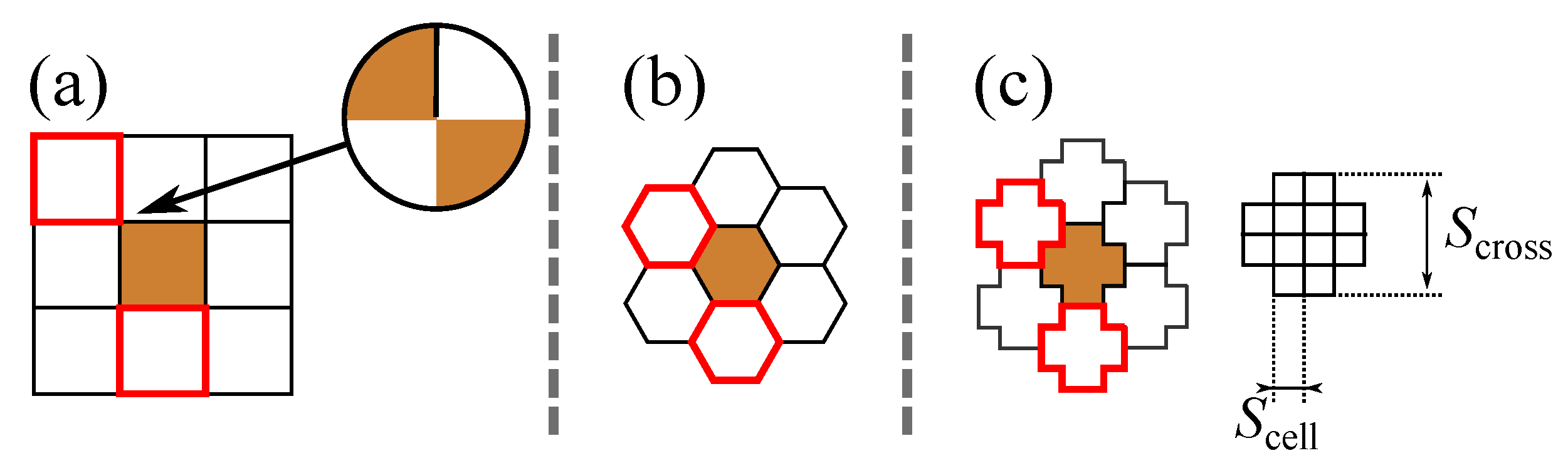
In order to achieve an automated optimization procedure using a genetic algorithm, a predefined area has to be subdivided into individual elements or pixels, as indicated in Figure 1. Each pixel is represented by a Boolean value that corresponds to a conductive or non-conductive element (0, 1). A conductive element, or “1”, is analogous to a 35 μm thick copper layer on top of the substrate (Rogers RO4350B). Although any geometrical shape can be used, crosses have been shown to be advantageous over rectangles and hexagons for mainly two reasons:

• Singularities: for rectangles, infinitesimally small connections between pixels can occur (Figure 1a). This can lead to a diminished simulation accuracy and also errors in measurements due to a limited production accuracy.
• Resolution: restriction to rectangular cells for the simulation mesh in certain software packages leads to errors due to the limited resolution of the angled sides in hexagons (Figure 1c).

Crosses exhibit no singularities and are ideal for simulation tools that employ rectangular cells. Every second row is shifted by half an element in order to avoid non-conducting areas between the crosses. The minimum resolution has been found to be 0.58% of the wavelength, i.e., a more refined mesh does not lead to improved simulation results.

2.2. Genetic Algorithm

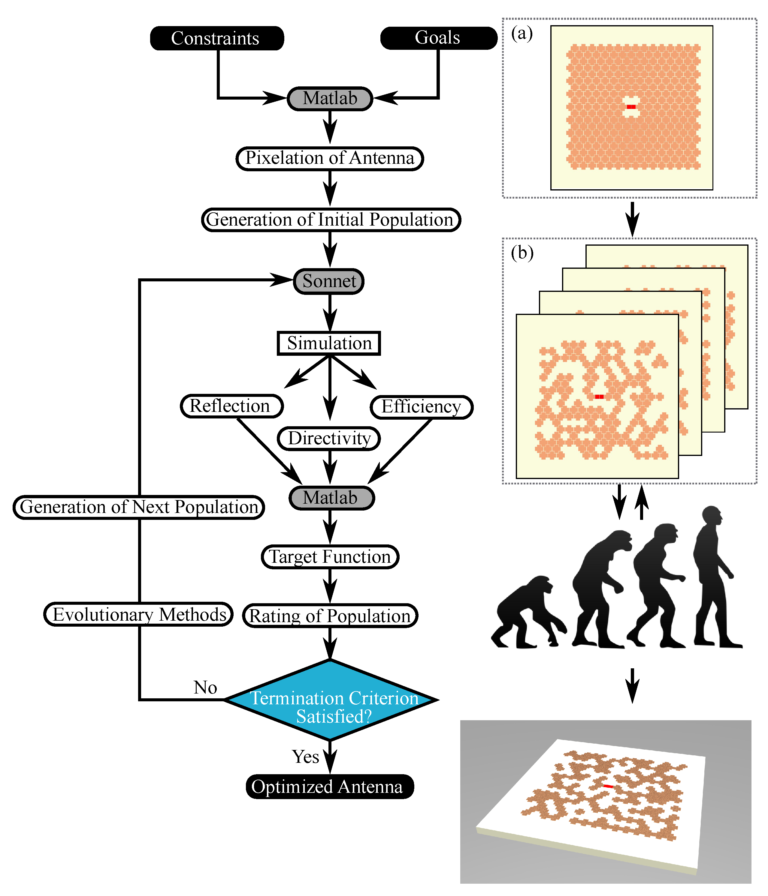
The basic principle of genetic algorithms, as shown in Figure 2, is the optimization of a problem through the continued improvement or evolution of individuals.

• Based on user input, a given antenna size is pixelated and a first, random, initial population with a uniform distribution of pixels (50% “0” and $50\%$ “1”) is generated in Matlab.
• This initial population is simulated with Sonnet Software, which has been chosen due to its fast computation time. Parameters needed for the calculation of a fitness function (i.e., reflection coefficient and gain or power) are simulated for each individual of the population and handed back to Matlab.
• The fitness function for each individual is computed from these simulated parameters, after which evolutionary methods such as selection, recombination and mutation are used to create a second population.
• The second population is again simulated with Sonnet Software.

This iterative process is repeated until either the termination criterion has been achieved (e.g., the desired optimization goal) or the maximum number of generations has been reached.

Post-optimization simulations are carried out employing full wave simulations with Ansys HFSS to cross-check the achieved results with Sonnet Software.

2.2.1. Antenna Parameters

In contrast to previous studies by the authors, instead of a low reflection coefficient S₁₁, the antenna gain or power are chosen as an optimization goal.

Both directivity, D, and gain, G, are a measure of the increase in emitted power over a reference antenna (isotropic antenna with uniform radiation in all spatial directions) in a specific direction.

The directivity function is defined as the ratio between the power per unit solid angle at a specific angle $U(\mathsf{\Theta },\phi )$ and the average radiated power per unit solid angle $P_{rad}/\left(4\pi \right)$ [23].

$$D(\mathsf{\Theta },\phi )=\frac{U(\mathsf{\Theta },\phi )}{\frac{1}{4\pi }{P}_{rad}}$$

(1)

The gain function additionally takes the radiation efficiency, ${\eta }_r$, into consideration [23].

$$G(\mathsf{\Theta },\phi )=\frac{U(\mathsf{\Theta },\phi )}{\frac{1}{4\pi }{P}_{rad}}{\eta }_r=D(\mathsf{\Theta },\phi ){\eta }_r$$

(2)

If not specified otherwise, the maximum value of Equation (1) is called the directivity and the maximum of Equation (2) is called the gain. Both are given in dBi when compared to an isotropic radiator.

The radiation efficiency can be defined as

$${\eta }_r=\frac{P_{rad}}{P_a}$$

(3)

with $P_a$ being the power accepted by an antenna, which can be written as:

$$P_a=P_t-P_r$$

(4)

where $P_r$ is the reflected power due to impedance mismatch and $P_t$ is the transmitted power to the antenna.

Using powers, the reflection coefficient S₁₁ can be defined as follows:

$$|S_{11}{|}^2=\frac{P_r}{P_t}$$

(5)

2.2.2. Symmetry Restriction

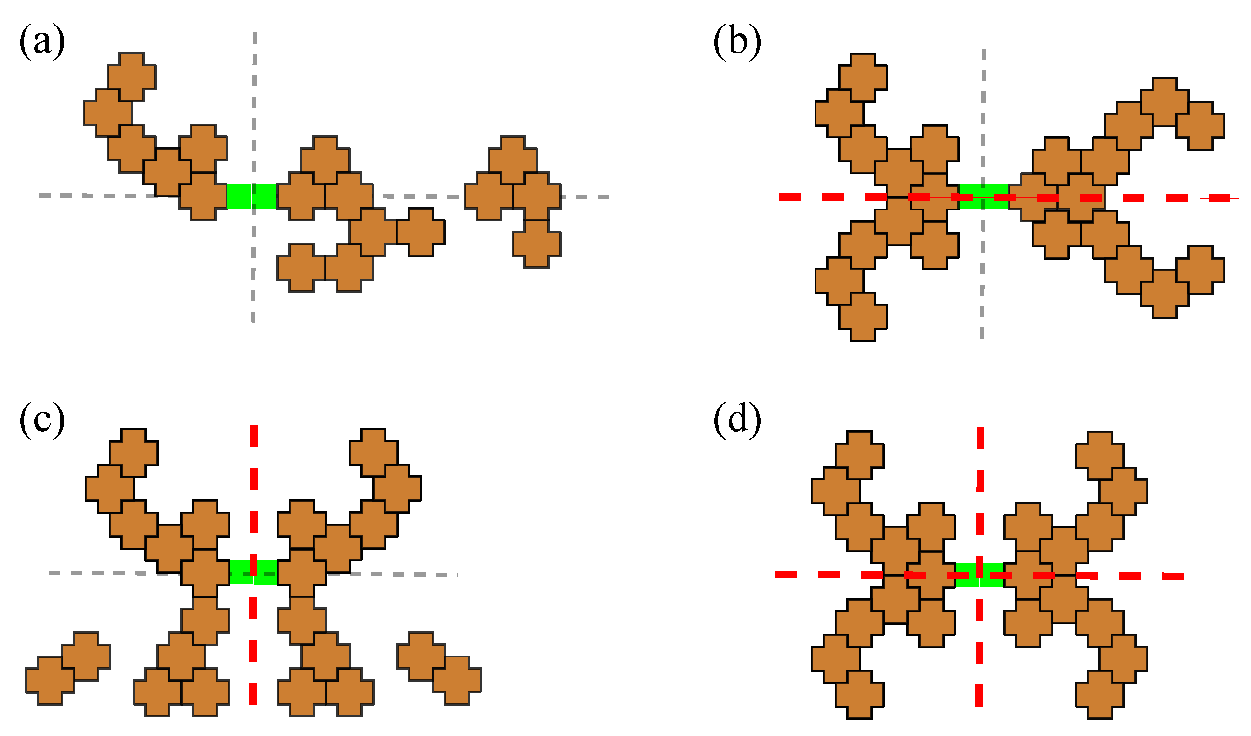
In order to study the influence of symmetry restrictions on an antenna’s performance, four distinct cases have to be distinguished:

(a)

Asymmetry: no symmetry restrictions are applied to the antenna;

(b)

x-symmetry: the antenna is symmetrical along the x-axis;

(c)

y-symmetry: the antenna is symmetrical along the y-axis;

(d)

xy-symmetry: the antenna is symmetrical along both axes.

Figure 3 shows exemplary representations of pixelated structures with different symmetries. The point of origin at (0, 0) in green indicates the antenna port, where differential feeding to the antenna is applied.

2.3. Measurement Procedure

Prior to the measurement, a VNA (Rohde und Schwarz, ZNB-8) is calibrated using through-open-short-match (TOSM) calibration (Rohde und Schwarz, ZV-Z170). For gain measurements, each antenna is measured twice (in the horizontal and vertical directions) to obtain the total system gain. In order to avoid pattern squint due to unbalanced currents, a Bazooka Balun is used, whose length is shorter than a quarter wavelength because of fringing fields at the open end of the balun [24].

Due to the balanced nature of the produced antennas, the method described by Qing et al. [25] is used to measure the impedance. The “direct compensation” standard de-embedding technique of the employed VNA is used, employing shorted fixture connectors to offset the influence of the test fixture.

3. Results

The main goal of this work was to design directional antennas. Antennas of different types were optimized following the process described above. Relevant data were collected for comparison in the following section. The antennas were optimized using gain or power in either the x-, y- or z-directions. The chosen operating frequency was 868 $\mathrm{M}$$\mathrm{Hz}$ for operation in the UHF RFID band.

The topologies implemented for this work were x-symmetrical, y-symmetrical and xy-symmetrical electrically large antennas, due to the ease of manufacture and short simulation times.

In order to describe the size of an antenna, the electrical size $ka$ is used, where k is the wavenumber ($2\pi /\lambda$) in radians per meter and a is the radius of a sphere at the antenna’s largest dimension.

$ka\le 1$ is often used as the threshold for electrically small antennas [26]; therefore, $ka>1$ describes electrically large antennas in this study.

3.1. Simulation Results

Table 1. Dimensions and electrical sizes of the groups of generated antennas.

Antenna	Dimensions/mm	Dimension/Pixels	Electrical Size
Asymmetrical	152.5 × 143.75	30 × 38	1.91
x symmetrical	152.5 × 140	30 × 37	1.88
y symmetrical	150 × 143.75	29 × 38	1.89
xy symmetrical	150 × 140	29 × 37	1.87

shows the physical dimensions and the electrical size of the various types of simulated antennas.

Apart from small deviations due to pixels deleted by the optimization process, the dimensions were kept the same within each group. The optimization options were kept identical across all simulations and are shown in Appendix A,

Table A1. Parameters used for the genetic algorithm function within Matlab.

Property	Value
Strings per Generation	50
Crossover Rate	0.8
Mutation Rate	0.01
Elite Count	2
MaxGenerations	200

. The exception is the method of calculating the fitness score, maximum power or maximum gain. The best antenna possible within the allotted generation limit is generated by giving the fitness function a goal it cannot reach.

The antennas were then investigated for the achieved maximum gain, their reflection coefficient at the operating frequency and the radiating direction of the main lobe with the deviation from the desired direction. The resolution of the gain patterns was examined in $5^{\circ }$ steps in the $\theta$ and $\varphi$ directions, as this delivers precise results in addition to a reasonable computing time.

Table A2. The gain, reflection coefficient, the direction with the deviation from the desired direction and the optimization goal of all antennas. For antennas optimized in z-direction, no deviation $d\Phi$ can be defined (˜).

Names	${\mathit{S}}_{11}$/dB	Gain/dB	$\mathbf{\Theta }$	$\mathit{d}\mathbf{\Theta }$	$\mathbf{\Phi }$	$\mathit{d}\mathbf{\Phi }$	Target Function
200914aSxO	−9.921	6.373	85	5	355	5	power
201012xSxO	−26.565	4.346	45	45	0	0	power
201020ySxO	−7.635	5.047	85	5	0	0	power
201021xSyO	−13.429	5.005	90	0	90	0	power
201023ySyO	−10.235	5.507	85	5	90	0	power
201106rSxO	−26.209	5.054	5	85	0	0	power
201220aSyO	−19.493	7.108	90	0	90	0	power
201223aSxO	−1.05	7.618	90	0	5	5	gain
201226aSyO	−5.295	6.435	90	0	90	0	gain
210109ySyO	−3.945	7.063	90	0	90	0	gain
210112aSxO	−10.305	6.326	90	0	5	0	power
210114aSyO	−7.409	5.601	85	5	95	5	power
210116rSyO	−8.094	6.184	90	0	90	0	power
210122aSxO	−11.141	5.953	90	0	15	15	power
210125aSyO	−9.048	5.993	90	0	90	0	power
210127aSzO	−23.978	3.783	10	10	225	˜	power
210203xSzO	−17.33	4.897	5	5	0	˜	power
210207ySzO	−22.709	3.57	10	10	270	˜	power
210308aSxO	−1.738	7.763	90	0	5	5	gain

in Appendix B shows these parameters at the desired resonance frequency of 868 $\mathrm{M}$$\mathrm{Hz}$, in addition to the used target function.

Table 2. Comparison of the calculated Chu–Harrington limit for each antenna type (G_CH), the maximum achieved gain (G_max) and the minimum achieved gain (G_min).

Antenna	GCH/dB	Gmax/dB	Gmin/dB
Asymmetrical	7.45	7.76	3.78
x symmetrical	7.31	7.24	4.35
y symmetrical	7.35	7.06	3.57
xy symmetrical	7.22	5.05	6.18

summarizes these results by showing the minimal and maximum achieved gain for each antenna symmetry compared to the theoretical gain according to the Chu–Harrington limit [27].

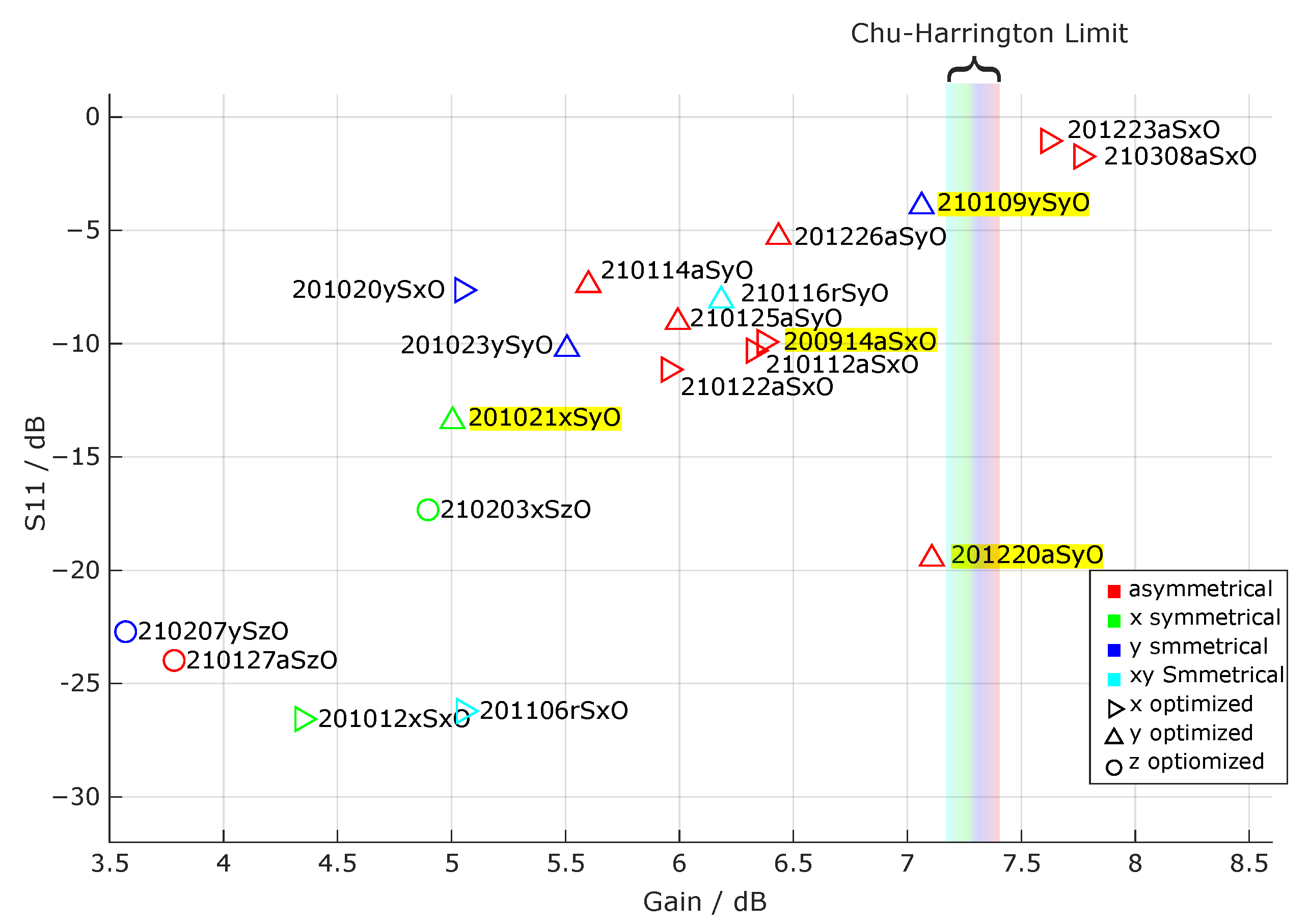
The results for gain and S₁₁ are shown in Figure 4, with the respective Chu–Harrington limit for the different antenna topologies. The employed nomenclature is Date-Symmetry-Direction of Optimization. The letter “r” for antenna symmetry designates radial symmetry, i.e., the xy symmetry. The colors of the data points in the plot indicate the symmetry of the optimized antennas, whereas the shapes of said data points signify the direction of optimization. Except for 210127aSzO, the gain of all asymmetrical antennas exceeds $5.5$ dBi. Conversely, all symmetrical antennas, with the exception of 210116rSyO and 210109ySyO, fall below this threshold.

Additionally, it can be seen from Table 2 in conjunction with Figure 4 that the only antennas surpassing the Chu–Harrington limit are 201223aSxO and 210308aSxO, which are asymmetric antennas optimized in the x-direction. The gains of all other antennas fall below their respective Chu–Harrington limit.

By looking at Table A2, it is apparent that all antennas with $S_{11}<-5 \mathrm{d}\mathrm{B}$ have been optimized using the power, $U(\mathsf{\Theta },\phi )$, and not the gain, $G(\mathsf{\Theta },\phi )$. This is due to the fact that the antenna gain is independent of S₁₁, but not the power $U(\mathsf{\Theta },\phi )$. Therefore, optimizing for $U(\mathsf{\Theta },\phi )$ inherently leads to better results for the reflection coefficient, whereas this parameter is not regarded when using $G(\mathsf{\Theta },\phi )$ as an optimization goal.

Consequently, in order to achieve a high gain and a low reflection coefficient, two possible strategies are possible:

• Optimizing for power;
• Multi-objective optimization to optimize an antenna using gain and S₁₁ as target functions at the same time. This method has already been successfully used to optimize pixelated antennas for submersion in dielectric materials in a recent study by the authors [28].

3.2. Measurement Results

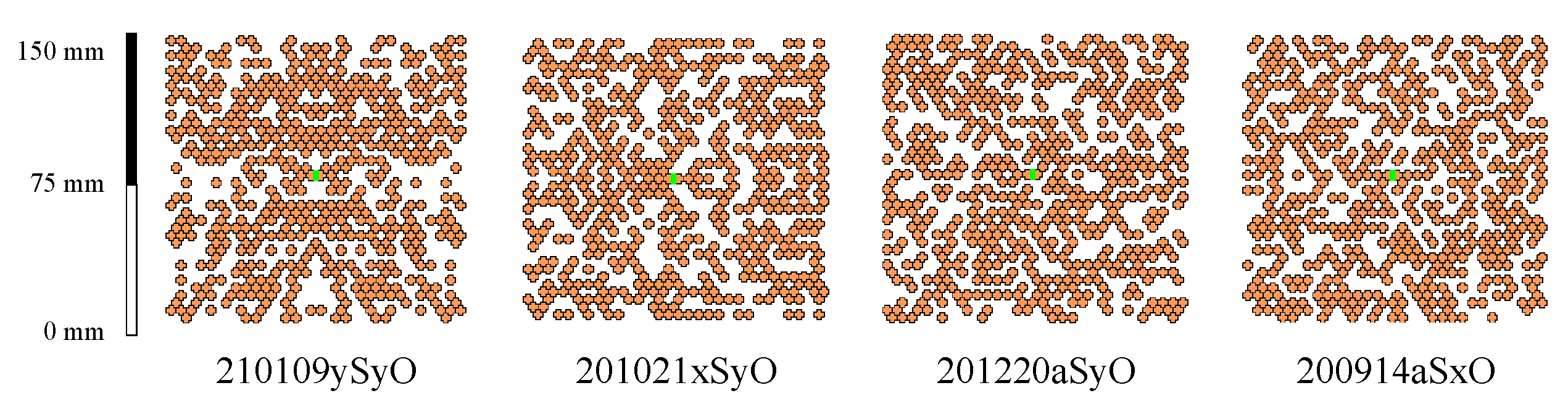
Four antennas were chosen for experimental verification based on their high gain and low reflection coefficients: two asymmetrical antennas (201220aSyO and 201111aSxO) and one antenna for each symmetry axis (y-symmetrical: 210109ySyO and x-symmetrical: 201021xSyO). The resulting topologies are shown in Figure 5.

The axial ratios of these presented topologies are 87 dB (210109ySyO), 72 dB (201021xSyO), 64 dB (201220aSyO) and 75 dB (201111aSxO), respectively, indicating a strong linear polarization.

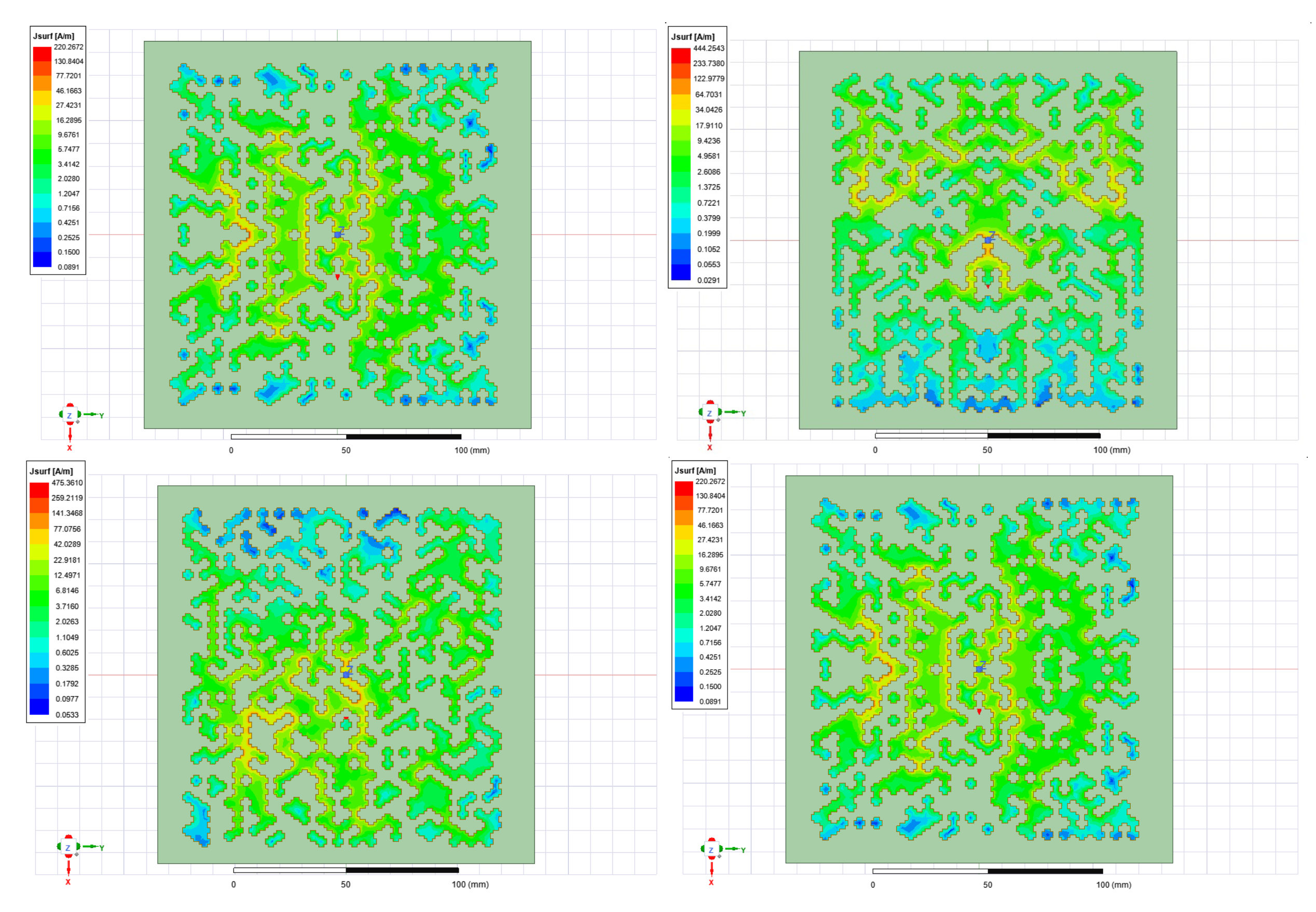
The gain patterns, the gain in the desired optimization direction and the S₁₁ of each antenna are shown compared to the simulation results. The gain patterns were measured at 868 $\mathrm{M}$$\mathrm{Hz}$. Surface current plots of the measured topologies are shown in Appendix C.

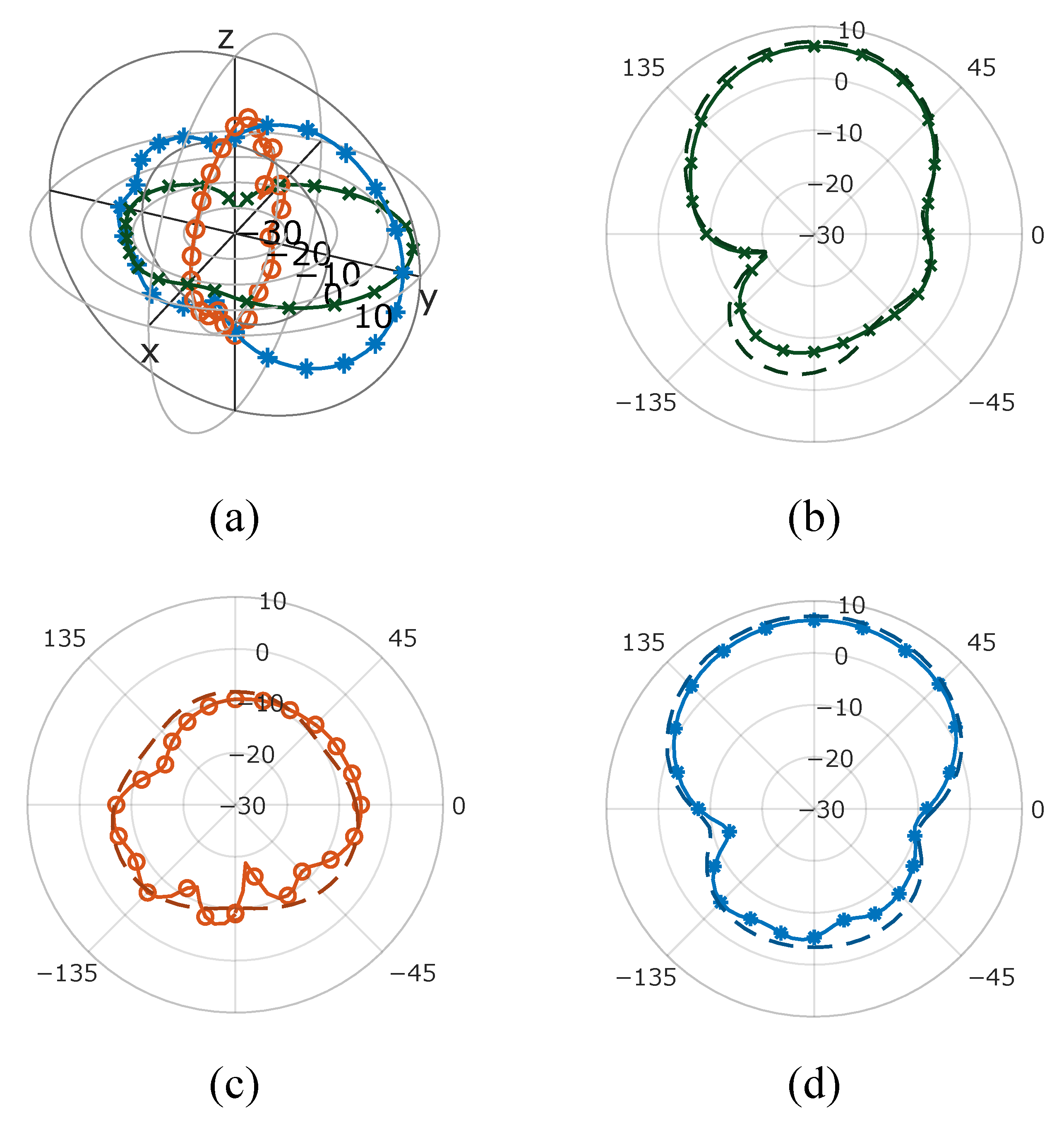
3.2.1. Antenna 210109ySyO

Gain Pattern

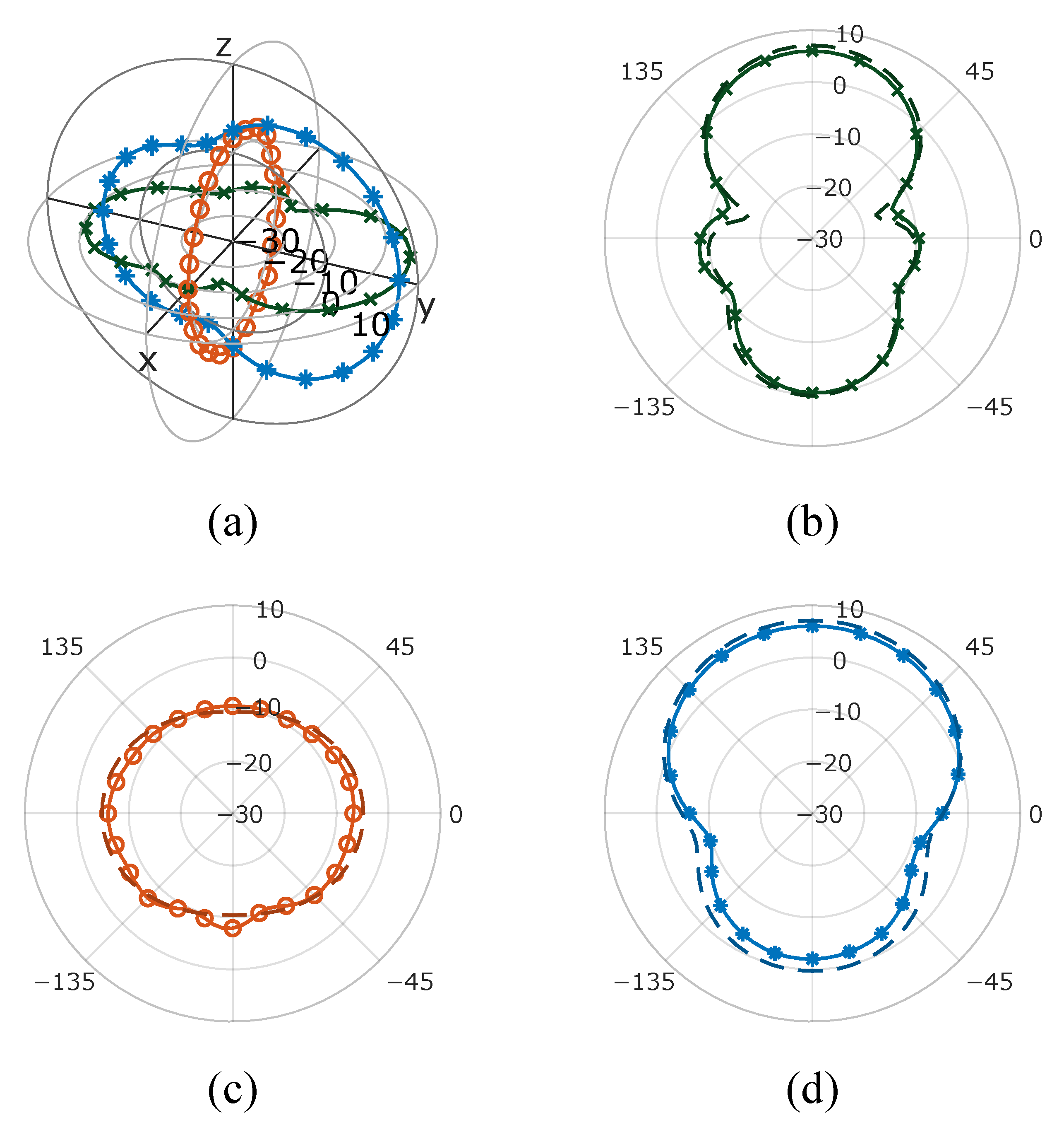
The measured and simulated data of 210109ySyO are in excellent agreement, as can be seen in Figure 6. Furthermore, the developed directivity matches the direction of optimization. The measured gain in the azimuth plane is $5.99$ dBi. The mean absolute error (MAE) of the gain pattern between measurement and simulation is $1.08$ dB.

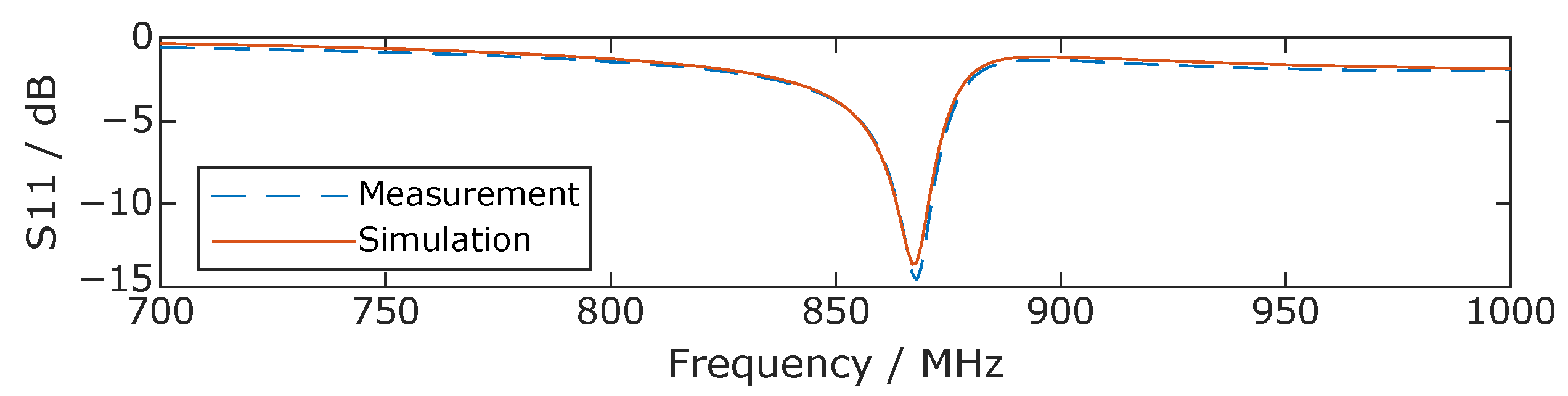
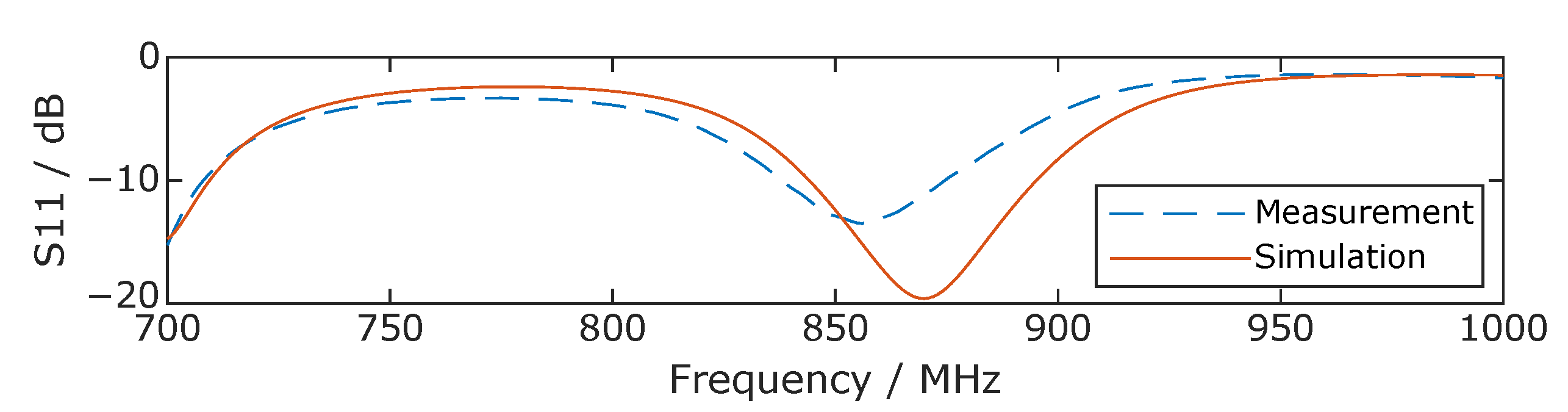
S₁₁ Parameter

The measured value of S₁₁ is $-16.98$ dB at a resonance frequency of $853.74$ $\mathrm{M}$$\mathrm{Hz}$, compared to the simulation value of $-15.62$ dB at $859.94$ $\mathrm{M}$$\mathrm{Hz}$, as seen in Figure 7. This corresponds to a deviation of only $0.7$ between measurement and simulation.

3.2.2. Antenna 201021xSyO

Gain Pattern

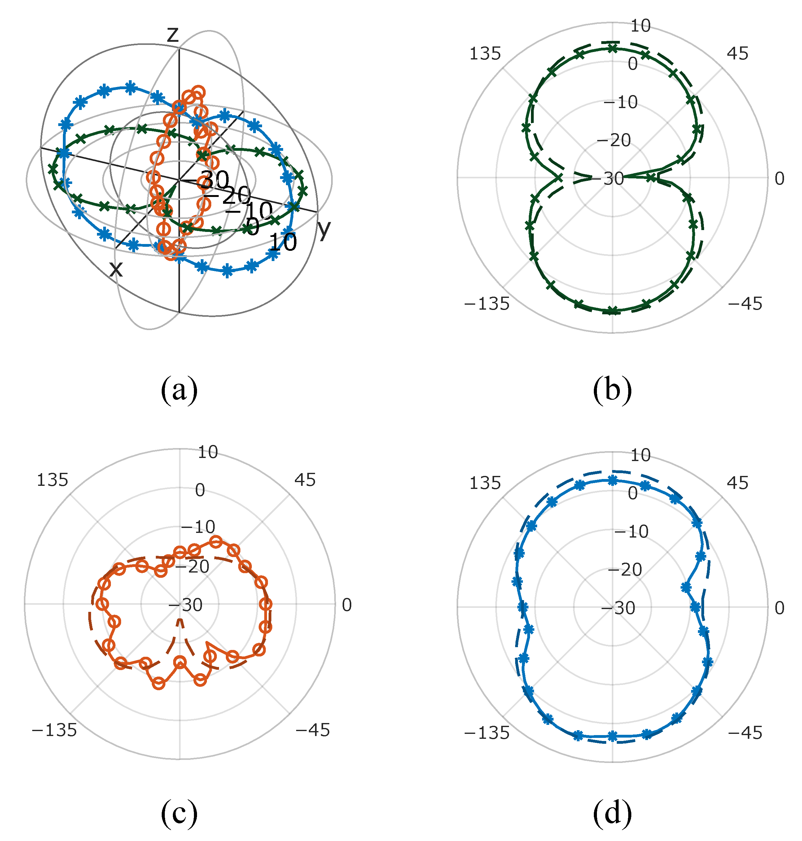
Again, the measurements match the simulation very well and the developed directivity matches the direction of optimization, as can be seen in Figure 8. The measured gain in the azimuth plane is $3.27$ dBi. The MAE of the gain pattern between measurement and simulation is $2.11$ dB.

S₁₁ Parameter

The measured and simulated S₁₁ of this antenna are close to being identical, as can be seen in Figure 9. The measured value of $S_{11}$ is $-14.52$ dB at a frequency of $867.7$ $\mathrm{M}$$\mathrm{Hz}$, compared to the simulated value of $867.11$ $\mathrm{M}$$\mathrm{Hz}$.

3.2.3. Antenna 201220aSyO

Gain Pattern

This antenna is asymmetrical and clearly develops a strong directiviy seen in Figure 10, with an overall excellent agreement between measurements and simulations. The measured gain in the elevation plane ($\varphi =90{}^{\circ }$) is $6.31$ dBi and the MAE of the gain pattern between measurement and simulation is $1.65$ dB.

S₁₁ Parameter

For this antenna, S₁₁ shows the largest deviation (in resonance and value), as seen in Figure 11. The measured value of S₁₁ is $-13.5$ dB at a resonance frequency of $855.74$ $\mathrm{M}$$\mathrm{Hz}$, compared to the simulation value of $-19.58$ dB at $869.79$ $\mathrm{M}$$\mathrm{Hz}$, which corresponds to a deviation of $1.6$% between measurement and simulation.

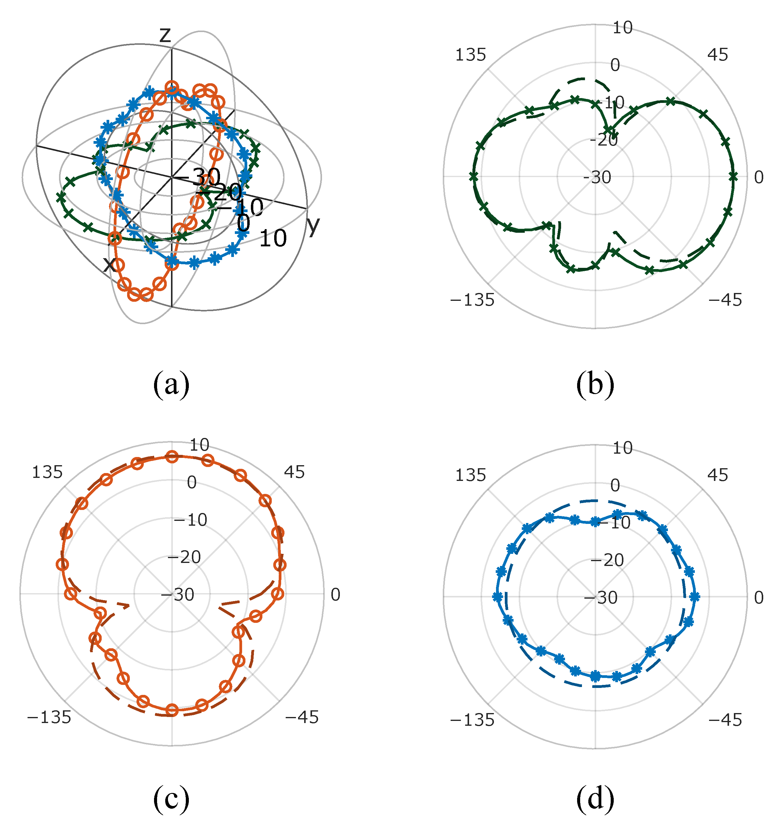
3.2.4. Antenna 200914aSxO

Gain Pattern

This antenna was optimized in the x-direction, which can be seen in Figure 12. Slight deviations can be detected in sections with a small gain. The measured gain in the elevation plane ($\varphi =0{}^{\circ }$) is $5.21$ dBi and the MAE of the gain pattern between measurement and simulation is $2.29$ dB.

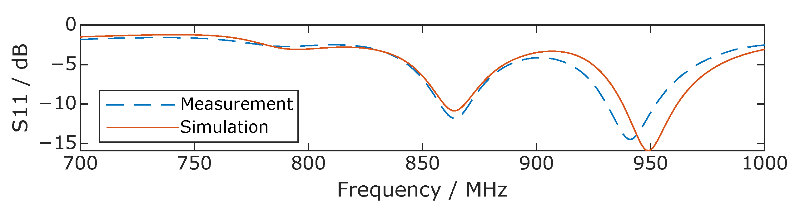
S₁₁ Parameter

This antenna developed two resonances in the pictured band. At the first resonance, the simulation and measurement match well, and at the second, a downshift in the minimum is visible, Figure 13. The measured value of S₁₁ is $-11.85$ dB at a resonance frequency of $863.73$ $\mathrm{M}$$\mathrm{Hz}$, compared to the simulated value of $-9.92$ dB at $864.03$ $\mathrm{M}$$\mathrm{Hz}$, which is a negligible deviation. The deviation for the second resonance (around 950 $\mathrm{M}$$\mathrm{Hz}$) is not discussed, since this was not an optimization goal.

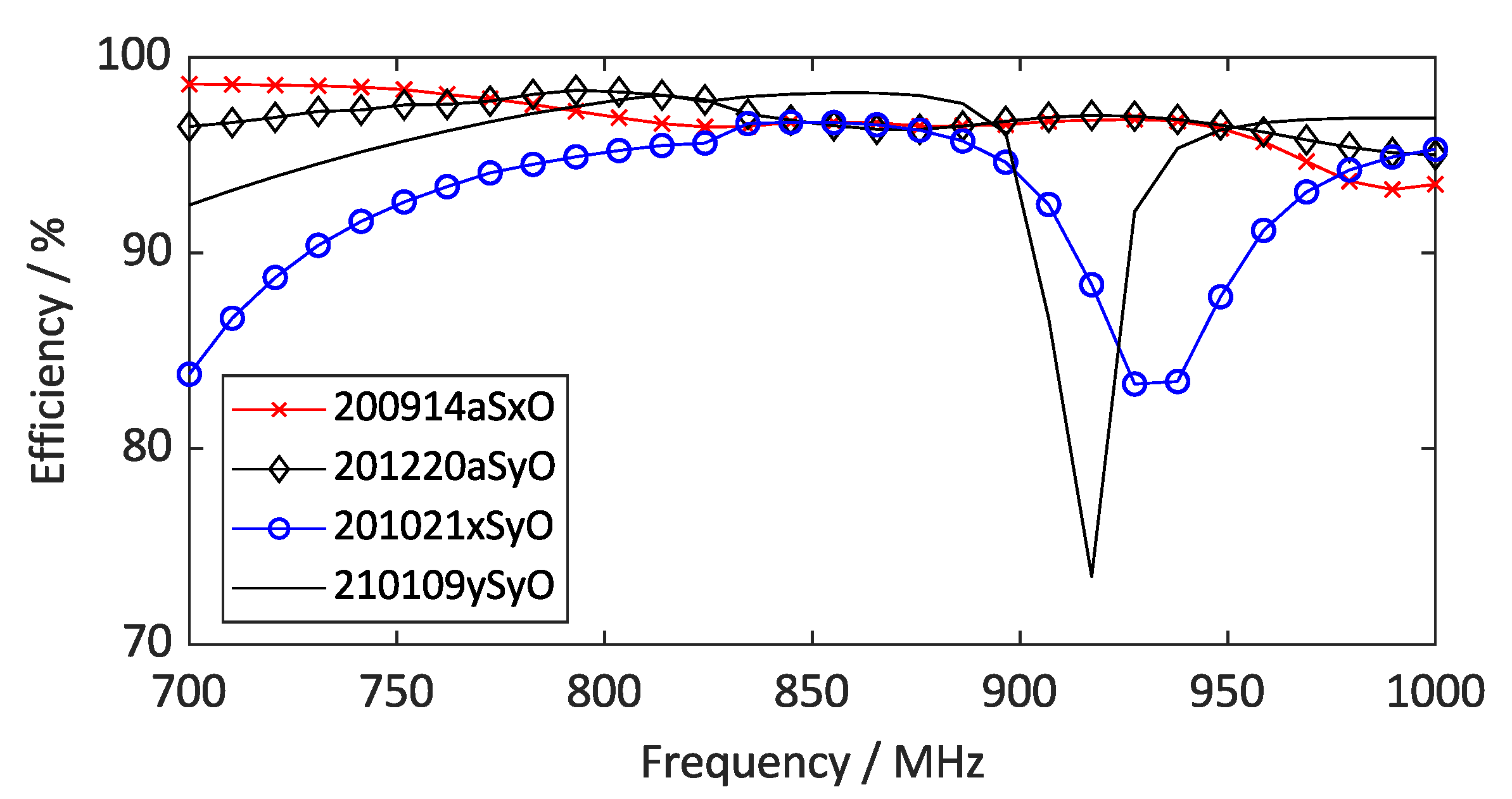
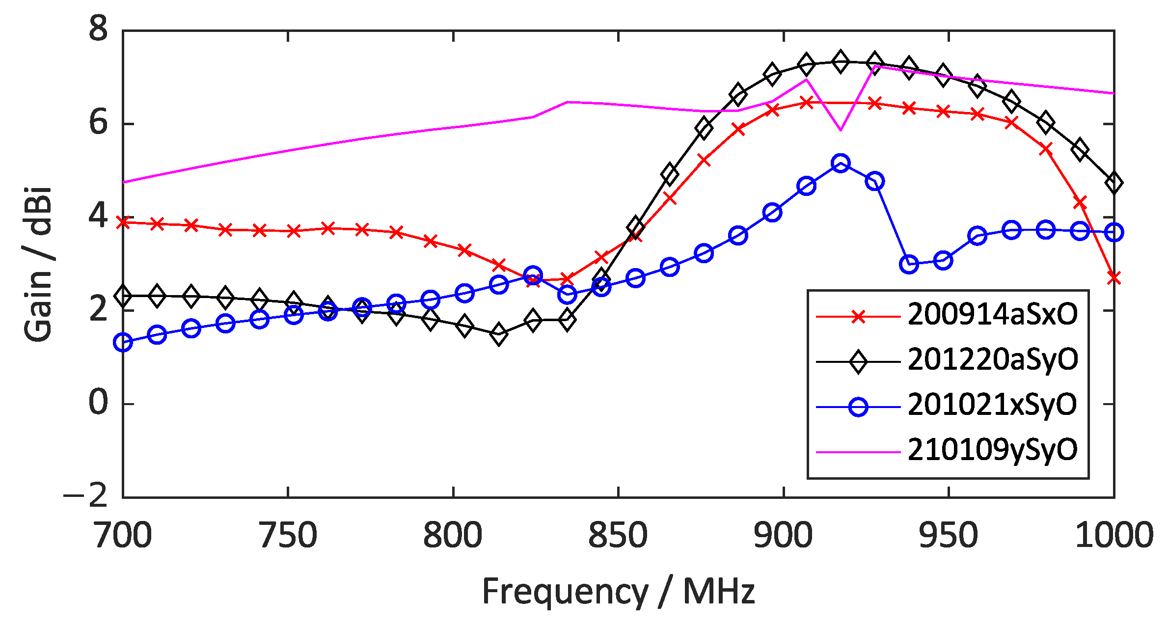
3.3. Gain and Radiation Efficiency as a Function of Frequency

Figure 14 and Figure 15 show the radiation efficiency and gain in the frequency range of 700 $\mathrm{M}$$\mathrm{Hz}$ to 1000 $\mathrm{M}$$\mathrm{Hz}$.

While the asymmetric antennas exhibit a consistent efficiency in the investigated frequency range, the symmetric antennas experience considerable dips around 917 $\mathrm{M}$$\mathrm{Hz}$ (210109ySyO) and 930 $\mathrm{M}$$\mathrm{Hz}$ (201021xSyO).

The asymmetric antennas exhibit a clear increase in gain starting from 835 $\mathrm{M}$$\mathrm{Hz}$. While the gain of the x-symmetric antenna also slightly increases at this frequency before decreasing again to 920 $\mathrm{M}$$\mathrm{Hz}$, the y-symmetric antenna shows a steady, high gain over the whole range.

A more detailed study on this behavior must be performed, possibly also employing multi-objective optimization in order to test these properties for a larger dataset. For just the four measured antennas, no clear statements about the influence of symmetry restrictions on the gain and radiation efficiency can be made. A common mode analysis of symmetric antennas might also yield additional information on the behaviour of the radiation efficiency for symmetric antennas.

Differences in the results for gain versus frequency and gain patterns shown in the previous paragraphs are due to the fact that the frequency dependence was simulated using Ansys, whereas the gain patterns were simulated using Sonnet due to the lower computation time.

4. Discussion

Overall, the simulated data match the measurement results very well, as extensively documented in Section 3.2. The errors between measured and simulated resonance frequencies are very small, with the highest deviation being 1.6%. The measured gain patterns match the simulated data very well, with the development of directional antennas in the desired direction of optimization. The simulation results were confirmed and the overall premise of the presented study, i.e., symmetry restrictions and their effects on the antenna gain, was shown to lead to interesting insights for pixelated antennas.

Optimizing for power or gain produces highly directional antennas, with gains close to the theoretical Chu–Harrington limit. This is the first report on pixelated antennas that have been specifically optimized for high gain by using either the gain or power as a target function in a genetic algorithm. A clear deviation in results is seen between choosing gain or power as the target function, where the latter can also produce well-matched antennas, i.e., those with a low S₁₁ and a high gain at the same time. Using the gain as an optimization goal leads to unsatisfying results for the reflection coefficient. As discussed in Section 3.1, this is due to the fact that the antenna gain is independent of S₁₁, whereas $U(\mathsf{\Theta },\phi )$ is not.

In order to achieve high-gain, well-matched antennas, optimizing for power is the method of choice when using single objective optimization. Multi-objective optimization of gain and reflection coefficients will be investigated in future studies.

Another possibility that has been shown in a different context for the design of a low-noise stable broadband microwave amplifier [29] is to use a hybrid optimization scheme. In the above study, a genetic algorithm was used in combination with a conjugate gradient method (CGM). While a CGM is not expected to be useful for the optimization of pixelated antennas due to the high dimensionality of the problem, a combination of different optimization methods might yield interesting results for pixelated antennas.

In addition to gain and power, symmetry restrictions were also investigated for antennas that are symmetrical along the x-, y- and xy-axes, and for antennas that have no symmetry restrictions. The results show that unrestricted optimization can lead to antennas that can outperform the Chu–Harrington limit. Therefore, symmetry restriction shows no benefit for electrically large antennas. The applicability of the reported results and their use for electrically small antennas will be studied in future investigations. In previous studies by the authors, it has been shown that electrically small antennas can be optimized for their reflection coefficient [21]. It can be expected that electrically small antennas will benefit from multi-objective optimization, leading to high gain while achieving a low S₁₁.

Another aspect that must be studied in the context of symmetry restrictions is the bandwidth. Preliminary results indicate that the simulated electrically large antennas have narrow bandwidths, but no detailed investigation has been undertaken thus far. While the presented results can be used for the design of other antennas for radio communication, such as for the $2.4$ $\mathrm{G}$$\mathrm{Hz}$ WiFi band, it must be investigated whether they also hold true for mm wave band (30 $\mathrm{G}$$\mathrm{Hz}$ to 300 $\mathrm{G}$$\mathrm{Hz}$) devices or if different symmetry effects will play a role in this wavelength regime.

This is the first report on the effects of symmetry restrictions on pixelated antennas that have been optimized using genetic algorithms. In conclusion, the optimization of pixelated antennas for gain, using the optimization goals of gain or power, produces highly directional antennas, with symmetry restrictions leading to no positive effect. An increased solution space for asymmetric antennas leads to high gain antennas with pronounced directivity, with measurement results confirming the extensive simulations.

References

- Squires, M.; Tao, X.; Elangovan, S.; Gururajan, R.; Zhou, X.; Acharya, U.R. A novel genetic algorithm based system for the scheduling of medical treatments. Expert Syst. Appl. 2022, 195, 116464. [Google Scholar] [CrossRef]
- Zhang, X.; Yang, C. Application of Multipopulation Genetic Algorithm in Industrial Special Clothing Design. Wirel. Commun. Mob. Comput. 2022, 2022, 1632063. [Google Scholar] [CrossRef]
- Marasco, G.; Piana, G.; Chiaia, B.; Ventura, G. Genetic Algorithm Supported by Influence Lines and a Neural Network for Bridge Health Monitoring. J. Struct. Eng. 2022, 148, 04022123. [Google Scholar] [CrossRef]
- Weile, D.; Michielssen, E. Genetic algorithm optimization applied to electromagnetics: A review. IEEE Trans. Antennas Propag. 1997, 45, 343–353. [Google Scholar] [CrossRef]
- Dong, J.; Li, Q.; Deng, L. Design of Fragment-Type Antenna Structure Using an Improved BPSO. IEEE Trans. Antennas Propag. 2018, 66, 564–571. [Google Scholar] [CrossRef]
- Jia, X.; Lu, G. A Hybrid Taguchi Binary Particle Swarm Optimization for Antenna Designs. IEEE Antennas Wirel. Propag. Lett. 2019, 18, 1581–1585. [Google Scholar] [CrossRef]
- Aldhafeeri, A.; Rahmat-Samii, Y. Brain storm optimization for electromagnetic applications: Continuous and discrete. IEEE Trans. Antennas Propag. 2019, 67, 2710–2722. [Google Scholar] [CrossRef]
- Haupt, R.L. Thinned arrays using genetic algorithms. IEEE Trans. Antennas Propag. 1994, 42, 993–999. [Google Scholar] [CrossRef]
- Ares-Pena, F.J.; Rodriguez-Gonzalez, J.A.; Villanueva-Lopez, E.; Rengarajan, S.R. Genetic algorithms in the design and optimization of antenna array patterns. IEEE Trans. Antennas Propag. 1999, 47, 506–510. [Google Scholar] [CrossRef]
- Thors, B.; Steyskal, H.; Holter, H. Broad-band fragmented aperture phased array element design using genetic algorithms. IEEE Trans. Antennas Propag. 2005, 53, 3280–3287. [Google Scholar] [CrossRef]
- Ouedraogo, R.O.; Tang, J.; Fuchi, K.; Rothwell, E.J.; Diaz, A.R.; Chahal, P. A tunable dual-band miniaturized monopole antenna for compact wireless devices. IEEE Antennas Wirel. Propag. Lett. 2014, 13, 1247–1250. [Google Scholar] [CrossRef]
- Trinh-Van, S.; Yang, Y.; Lee, K.Y.; Hwang, K. A Wideband Circularly Polarized Pixelated Dielectric Resonator Antenna. Sensors 2016, 16, 1349. [Google Scholar] [CrossRef] [Green Version]
- Mair, D.; Unterladstaetter, M.; Renzler, M.; Ussmueller, T. Evolutionary Optimized Pixelated Antennas for 5G IoT Communication. In Proceedings of the 2022 52nd European Microwave Conference (EuMC), Milan, Italy, 27–29 September 2022; IEEE: New York, NY, USA, 2022. [Google Scholar] [CrossRef]
- Derbal, M.C.; Zeghdoud, A.; Nedil, M. A Novel Dual Band Antenna Design for WiFi Applications Using Genetic Algorithms. In Proceedings of the 2018 IEEE International Symposium on Antennas and Propagation & USNC/URSI National Radio Science Meeting, Boston, MA, USA, 8–13 July 2018; IEEE: New York, NY, USA, 2018. [Google Scholar] [CrossRef]
- Dhakshinamoorthi, M.K.; Gokulakkrizhna, S.; Denesh Kumar, M.; Subha, M.; Mekaladevi, V. Rectangular Microstrip Patch Antenna Miniaturization using improvised Genetic Algorithm. In Proceedings of the 2020 4th International Conference on Trends in Electronics and Informatics (ICOEI)(48184); Tirunelveli, India, 15–17 June 2020, IEEE: New York, NY, USA, 2020. [Google Scholar] [CrossRef]
- Jayasinghe, J.; Uduwawala, D. Optimization of the performance of patch antennas using genetic algorithms. J. Natl. Sci. Found. Sri Lanka 2013, 41, 113. [Google Scholar] [CrossRef] [Green Version]
- Chiu, Y.H.; Chen, Y.S. Multi-objective optimization for UWB antennas in impedance matching, gain, and fidelity factor. In Proceedings of the 2015 IEEE International Symposium on Antennas and Propagation & USNC/URSI National Radio Science Meeting, Vancouver, BC, Canada, 19–24 July 2015; IEEE: New York, NY, USA, 2015. [Google Scholar] [CrossRef]
- Steyskal, H. On the Merit of Asymmetric Phased Array Elements. IEEE Trans. Antennas Propag. 2013, 61, 3519–3524. [Google Scholar] [CrossRef]
- Song, C.; Huang, Y.; Zhou, J.; Carter, P.; Yuan, S.; Xu, Q.; Fei, Z. Matching Network Elimination in Broadband Rectennas for High-Efficiency Wireless Power Transfer and Energy Harvesting. IEEE Trans. Ind. Electron. 2017, 64, 3950–3961. [Google Scholar] [CrossRef] [Green Version]
- McLean, J.S.; Foltz, H.D. Symmetry Versus Balance in Balancing Networks for Dipolar Antennas. IEEE Trans. Electromagn. Compat. 2020, 62, 1406–1418. [Google Scholar] [CrossRef]
- Mair, D.; Renzler, M.; Pfeifhofer, A.; Ußmüller, T. Evolutionary optimization of asymmetrical pixelated antennas employing shifted cross shaped elements for UHF RFID. Electronics 2020, 9, 1856. [Google Scholar] [CrossRef]
- Sonnet. SonnetLab. 2023. Available online: https://www.sonnetsoftware.com/support/sonnet-suites/sonnetlab.html (accessed on 25 January 2023).
- Volakis, J.L. Antenna Engineering Handbook, 4th ed.; McGraw-Hill Professional: New York, NY, USA, 2007. [Google Scholar]
- Saario, S.A.; Lu, J.W.; Thiel, D.V. Full-wave analysis of choking characteristics of sleeve balun on coaxial cables. Electron. Lett. 2002, 38, 304–305. [Google Scholar] [CrossRef] [Green Version]
- Qing, X.; Goh, C.K.; Chen, Z.N. Impedance Characterization of RFID Tag Antennas and Application in Tag Co-Design. IEEE Trans. Microw. Theory Tech. 2009, 57, 2017288. [Google Scholar] [CrossRef]
- Wheeler, H.A. Fundamental limitations of small antennas. Proc. IRE 1947, 35, 1479–1484. [Google Scholar] [CrossRef]
- Harrington, R.F. Effect of antenna size on gain, bandwidth, and efficiency. J. Res. Nat. Bur. Stand 1960, 64, 1–12. [Google Scholar] [CrossRef]
- Mair, D.; Fischer, M.; Konzilia, J.; Renzler, M.; Ussmueller, T. Evolutionary Optimization of Antennas for Structural Health Monitoring. IEEE Access 2023, 11, 4905–4913. [Google Scholar] [CrossRef]
- Shirkolaei, M.M. A New Design Approach of Low-Noise Stable Broadband Microwave Amplifier Using Hybrid Optimization Method. IETE J. Res. 2020, 68, 4160–4166. [Google Scholar] [CrossRef]
Figure 1.
Possible connections between elements of different shapes: (a) rectangles, (b) hexagons and (c) crosses, where red elements show vertical and diagonal neighbors. Diagonal elements can result in singularities due to a (theoretically) infinitesimally small connection (a), whereas for vertically spaced elements no singularities occur (b,c). For cross-shaped elements, the cross size (SCross) is defined as well as its separation into different Sonnet Software cells with size Scell (c).
Figure 2.
Flowchart of the proposed optimization technique. Initially, a predefined area is pixelated (a), after which an initial population is created with Matlab (b). After simulation with Sonnet, the fitness function is computed in Matlab. The population is rated and if it does not meet the termination criteria, a new one is created based on the first optimization.
Figure 3.
Examples of the different antennas: asymmetrical (a), symmetrical along the x-axis (b), symmetrical along the y-axis (c) and symmetrical along both x- and y-axes (d). The dashed red lines indicate the symmetry axes. The green elements in the center of the antenna indicate the antenna port.
Figure 4.
Gain and S11 for all optimized antenna structures with their respective symmetry and direction of optimization. The antennas chosen for measurement are highlighted.
Figure 5.
Topologies of the measurements chosen for experimental verification. The green squares indicate the feeding.
Figure 6.
(a) Gain pattern of 210109ySyO in 3D, (b) the azimuth plane and (c) the elevation plane at and (d) at (measurement: ― simulation: - - -).
Figure 7.
S11 of 210109ySyO between 700 MHz and 1 GHz.
Figure 8.
(a) Gain pattern of 210109xSyO in 3d, (b) the azimuth plane and (c) the elevation plane at and (d) at (measurement: ― simulation: - - -).
Figure 9.
S11 of 201021xSyO between 700 MHz and 1 GHz.
Figure 10.
(a) Gain pattern of 201220aSyO in 3d, (b) the azimuth plane and (c) the elevation plane at and (d) at (measurement: ― simulation: - - -).
Figure 11.
S11 of 201220aSyO between 700 MHz and 1 GHz.
Figure 12.
(a) Gain pattern of 200914aSxO in 3d, (b) the azimuth plane and (c) the elevation plane at and (d) at (measurement: ― simulation: - - -).
Figure 13.
S11 of 200914aSxO between 700 MHz and 1 GHz.
Figure 14.
Radiation efficiency as a function of frequency.
Figure 15.
Gain as a function of frequency.