Circuit Complexity in Interacting Quenched Quantum Field Theory

Abstract

In this work, we explore the effects of quantum quenching on the circuit complexity of quenched quantum field theory with weakly coupled quartic interactions. We use the invariant operator method under a perturbative framework to compute the ground state of this system. We give the analytical expressions for specific reference and target states using the ground state of the system. Using a particular cost functional, we show the analytical computation of circuit complexity for the quenched and interacting field theory. Furthermore, we give a numerical estimate of circuit complexity with respect to the quench rate, $\delta t$, for two coupled oscillators. The parametric variation in the unambiguous contribution of the circuit complexity for an arbitrary number of oscillators has been studied with respect to the dimensionless parameter $(t/\delta t$). We comment on the variation in the circuit complexity for different values of coupling strength, different numbers of oscillators and even in different dimensions.

1. Introduction

The quest to understand the fundamental laws of nature has driven research in both high energy physics and quantum information theory, leading to a remarkable interplay between these fields. By applying information-theoretic tools to the study of various quantum systems, researchers have made groundbreaking discoveries, revealing the deep connections between seemingly disparate areas of physics [1,2,3,4,5,6,7]. As we continue to explore the interconnections between these fields, we can look forward to new insights and discoveries that have the potential to transform our understanding of the universe.

Circuit complexity is a fundamental concept in quantum information theory that studies the computational resources required to solve a problem using quantum circuits. Formally, circuit complexity measures the minimum number of gates required to implement a given quantum computation as a function of the size of the input. The study of circuit complexity plays a crucial role in designing efficient quantum algorithms and understanding the power and limitations of quantum computers.

Since Leonard Susskind and their collaborators proposed the use of circuit complexity to study the interior of black holes [8,9,10,11,12,13,14,15], this approach has been extended to the study of quantum field theories. Researchers have found that circuit complexity can provide a useful tool for characterizing the complexity of entangled states in these theories and understanding their dynamics [16,17,18,19].

In the realm of many-body physics, the study of quantum quenches has become increasingly important in recent years, as it offers a powerful way to drive systems out of equilibrium and explore their dynamics [20,21,22]. In a quantum quench, a time-dependent parameter is suddenly or slowly varied, driving the system away from its ground state and potentially leading to thermalization. The study of entanglement in the context of quenched systems has been a key area of investigation [23,24,25,26,27,28,29,30,31,32]. Moreover, the measurement of circuit complexity in quenched systems has emerged as a valuable tool for quantifying the computational resources required to simulate their dynamics [33,34]. Together, these studies shed light on the fundamental principles of non-equilibrium dynamics in quantum systems, and may pave the way for the development of novel quantum technologies.

In dynamical systems, the time-dependent Schrödinger equation plays a crucial role in understanding their evolution over time. To tackle this problem, the Lewis–Resenfeld invariant operator method has been developed, which allows one to determine the time-dependent eigenstates of such systems [35]. Additionally, the method can be extended to consider the adiabatic evolution of time-dependent parameters [36,37], providing a means to compute time-independent perturbative corrections to the eigenstates [38]. The exact form of time-dependent parameters in these eigenstates can be found by solving the Ermakov–Milne–Pinney equation, which can be efficiently computed using the Mathematica software. These methods offer a powerful means to investigate the behavior of dynamical systems, shedding new light on the intricate interplay between their time-dependent parameters and their evolution over time.

In this research article, we investigate the circuit complexity of an interacting (quartic) quenched quantum field theory using the invariant operator method as described in the appendix of our previous work [39]. The quench protocol we employ is the most commonly studied in the literature, and we use the results of [19] based on Nielsen’s geometric approach to compute the circuit complexity. Specifically, we focus on graphically representing the time evolution of the unambiguous contribution of circuit complexity under different parametric variations. Our findings contribute to the growing body of literature on circuit complexity in quantum field theory and provide insights into the dynamics of complex interacting systems. For more details on the chosen quench protocol and methodology, readers can refer to [19,33,40].

The organization of the paper is as follows:

• Discretising quantum field theory (QFT) with quartic interaction on a lattice, we decouple the Hamiltonian using Fourier modes in Section 2. Evidently, the decoupled Hamiltonian refers to that of N coupled oscillators having a quartic perturbative coupling. The frequency of these oscillators is quenched by choosing a particular protocol.
• In Section 3, we use the invariant operator method to compute the time-dependent ground states and also the first-order perturbative corrections to the ground state of the quenched Hamiltonian. Notably, our research article represents the first time that this method has been applied to the computation of circuit complexity in quenched field theory. This innovative approach allows for a more comprehensive understanding of the dynamics of complex interacting systems and provides new insights into the behavior of circuit complexity under quenched conditions.
• Using the ground, we fix a specific reference and target state in Section 4. We then evaluate the circuit complexity of the chosen reference and target state in interacting (quartic) quenched quantum field theory using a particular cost function. We also evaluate the continuum limit of circuit complexity. Our results are based on a modification of the results presented in [19], which is founded on Nielsen’s geometric approach [41,42,43,44]. The method we use is more general than the covariance matrix approach used in [33] and is, therefore, applicable in a perturbative framework.
• In Section 5, we numerically evaluate circuit complexity for different sets of parameters and comment on the dynamical behavior of the circuit complexity in three different regimes.
• Section 6 encapsulates the conclusions we draw from the results obtained in this work.

2. The Setup and the Quench Protocol

While the effect of quenching on free field theories has been previously studied, this is one of the first attempts to understand its impact in the context of interacting theory. To begin, we focus on a scalar field theory with the $\widehat{\lambda }{\varphi }^4$ interaction term, which we regulate by placing it on a lattice. Once discretized, the Hamiltonian represents a family of N coupled anharmonic oscillators. We transform the original coordinates to normal modes to decouple the Hamiltonian, which allows us to compute the eigenstates for the system in a simpler way. To facilitate comparison with previous works, we follow the notations used in [16,19]. We also describe the time-dependent quench profile chosen, which is the frequency of these oscillators. The Hamiltonian for scalar field theory with a $\widehat{\lambda }{\varphi }^4$ interaction is given by [16],

$$\begin{array}{cc}\hfill \mathcal{H}=\frac{1}{2}\int d^{d-1}x& \left[\pi {\left(x\right)}^2+{(\nabla \varphi \left(x\right))}^2+m^2\varphi {\left(x\right)}^2+\frac{\widehat{\lambda }}{12}\varphi {\left(x\right)}^4\right],\hfill \end{array}$$

(1)

where d contains the space-time dimensions. We assume the coupling $\widehat{\lambda }<<1$, so that we can work in a perturbative framework. This theory can be discretized on a $d-1$ dimensional lattice, which is characterized by a lattice spacing $\delta$.

Closely following the prescription shown in [16,19] by making proper substitutions one can show that the Hamiltonian for scalar field theory having quartic interaction term can be expressed as,

$$\begin{array}{cc}\hfill \mathcal{H}=& \sum _{\overrightarrow{n}}\left\{\frac{\widehat{P}{\left(\overrightarrow{n}\right)}^2}{2M}+\frac{1}{2}M\left[{\omega }^2\widehat{X}{\left(\overrightarrow{n}\right)}^2+{\eta }^2\sum _i{\left(\widehat{X}\left(\overrightarrow{n}\right)-\widehat{X}\left(\overrightarrow{n}-{\widehat{x}}_i\right)\right)}^2+2\lambda \widehat{X}{\left(\overrightarrow{n}\right)}^4\right]\right\},\hfill \end{array}$$

(2)

where $\overrightarrow{n}$ denotes the spatial location of the points on the lattice, ${\widehat{x}}_i$ represents the unit vectors along the lattice, $\omega$ represents the frequency of individual oscillators and $\eta$ denotes inter-mass coupling. The above Hamiltonian in Equation (2) represents a family of infinitely coupled anharmonic oscillators. We use normal mode coordinates as a discrete Fourier transform of the original coordinates, given by:

$$x_a=\frac{1}{\sqrt{N}}\sum _{k=0}^{N-1}exp\left[i\frac{2\pi a}{N}k\right]{\tilde{x}}_k$$

(3)

$$p_a=\frac{1}{\sqrt{N}}\sum _{k=0}^{N-1}exp\left[i\frac{2\pi a}{N}k\right]{\tilde{p}}_k$$

(4)

Setting $M=1$ for simplicity, the Hamiltonian of Equation (2) can be rewritten in normal modes as:

$$\begin{array}{c}\hfill H=H_k+H_{{\varphi }^4}^{\prime },\end{array}$$

(5)

where

$$\begin{array}{c}\hfill H_k=\frac{1}{2}\sum _{k=0}^{N-1}\left[|{\tilde{p}}_k{|}^2+{\omega }_k^2{\left|{\tilde{x}}_k\right|}^2\right]\end{array}$$

(6)

denotes the unperturbed (free) Hamiltonian which can be decoupled for each of the N oscillators. Here,

$${\omega }_k^2={\omega }^2+4{\eta }^2{sin}^2\left(\frac{\pi k}{N}\right)$$

(7)

denotes the frequency for each of the N oscillators. The exact form of the eigenstates for the unperturbed Hamiltonian of Equation (6) has been computed in Section 3.1.

On the other hand, the $\lambda {\varphi }^4$ perturbation term in the Hamiltonian of Equation (5) can be dealt with by transforming the form of perturbations in normal modes:

$$\begin{array}{c}\hfill H_{{\varphi }^4}^{\prime }=\frac{\lambda }{N}\sum _{k_1,k_2,k_3=0}^{N-1}{\tilde{x}}_{\alpha }{\tilde{x}}_{k_1}{\tilde{x}}_{k_2}{\tilde{x}}_{k_3};\\ \hfill \alpha =N-k_1-k_2-k_3\mathrm{mod}N\end{array}$$

(8)

The contribution of the above Hamiltonian in Equation (8) is evaluated by approximating the first-order correction to the eigenstates of the unperturbed Hamiltonian by employing the use of time-independent perturbation theory in Section 3.2.

We now consider the frequency, $\omega$, in Equation (7) as a time-dependent quench profile. One of the most common quench profiles used in the literature [40] is given by:

$${\omega }^2(t/\delta t)={\omega }_0^2\left[{tanh}^2\left(\frac{t}{\delta t}\right)\right],$$

(9)

where ${\omega }_0$ can be considered as a free parameter and $\delta t$ measures the quench rate. We choose this particular quench profile since it admits an exact solution for the mode functions given in [40]. Note that this profile attains a constant value at very early and late time. Furthermore, for this chosen form of quench profile, dynamical changes in the system occur in the time window $[-\delta t,\delta t]$. We will set $t/\delta t=T$ and ${\omega }_0=1$. The respective frequencies in the normal mode basis take the following form,

$${\omega }_k=\sqrt{\omega {\left(T\right)}^2+4{\eta }^2{sin}^2\left(\frac{\pi k}{N}\right)},$$

(10)

where $\omega \left(T\right)$ is the quench profile in Equation (9) and k runs from 0 to $N-1$.

As the frequency of each oscillator now depends on time, the unperturbed Hamiltonian is evidently time-dependent. We employ the use of the invariant operator method to compute the exact form of the unperturbed Hamiltonian. We emphasize that the perturbed Hamiltonian is not time-dependent and hence can be used as a time-independent perturbation applied to N coupled oscillators. Using the ground state of the total Hamiltonian of Equation (5), we construct the reference as well as target states, which are further used to evaluate the circuit complexity of this interacting quench model.

3. Constructing a Wave Function for a ${\mathbf{\varphi }}^{\mathbf{4}}$ Quench Model

In this section, our prime objective is to derive an analytical expression for the eigenstates of the Hamiltonian in Equation (5) by using the Lewis–Resenfield invariant operator method and approximate it to the first-order perturbative correction. The expression for eigenstates of the decoupled and unperturbed Hamiltonian in Equation (6) is derived using the invariant operator method in Section 3.1. The first order perurbative correction to the ground state of the decoupled Hamiltonian is derived in Section 3.2.

3.1. Eigenstates and Eigenvalues for Unperturbed Hamiltonian

As shown earlier, in the normal mode basis, the unperturbed Hamiltonian of Equation (6) for N oscillators is decoupled. The wavefunction for any generic state of the N oscillators is then a product of the eigenstates for each decoupled Hamiltonian of Equation (6):

$$\begin{array}{c}\hfill {\psi }_{n_0\cdots n_{N-1}}\left({\tilde{x}}_0,\cdots {\tilde{x}}_{N-1},T\right)={\psi }_{n_0}({\tilde{x}}_0,T){\psi }_{n_1}({\tilde{x}}_1,T)\cdots {\psi }_{n_{N-1}}({\tilde{x}}_{N-1},T).\end{array}$$

(11)

where T denotes the time dependence of the eigenstates, emerging due to the quenched frequency in Equation (9). We deal with these time-dependent eigenstates by employing the use of the invariant operator method, closely following the method of [45]. In Appendix A, we have briefly mentioned the steps one can follow to compute an analytical expression for the eigenstates of a quenched Hamiltonian of Equation (6) using the invariant operator method. Using Equation (A11) and the arguments given in Appendix A, one can show that the expression for the eigenstate of the total unperturbed Hamiltonian of N coupled oscillators is:

$$\begin{array}{c}\hfill {\psi }_{n_1\cdots n_{N-1}}^{\left(0\right)}=\left(\frac{1}{2^{n_0+n_1+\cdots +n_{N-1}}{n}_0!\cdots n_{N-1}!}\right){\left(\frac{g_0{g}_1\cdots g_{N-1}}{{\pi }^N}\right)}^{1/4}exp\left[-\frac{i}{2}\sum _{k=0}^{N-1}(2n_k+1){\gamma }_k\right]exp\left[-\frac{1}{2}\sum _{k=0}^{N-1}{\tilde{\nu }}_k{\tilde{x}}_k^2\right]\\ \hfill \times {\mathbf{H}}_{n_0}\left[\sqrt{\dot{{\gamma }_0}}{\tilde{x}}_0\right]\cdots {\mathbf{H}}_{n_{N-1}}\left[\sqrt{{\dot{\gamma }}_{N-1}}{\tilde{x}}_{N-1}\right]\end{array}$$

(12)

where $g_k={\dot{\gamma }}_k$ and

$${\tilde{\nu }}_k={\dot{\gamma }}_k\left(1-\frac{i\dot{{\rho }_k}}{{\rho }_k\dot{{\gamma }_k}}\right)$$

(13)

for $k=0,1\cdots ,N-1$. All other symbols used in Equation (12) are defined in Appendix A. In this work, we focus on the ground state of the wavefunction shown in Equation (12), which can be written as:

$$\begin{array}{c}\hfill {\psi }_{0\cdots 0}^{\left(0\right)}={\left(\frac{g_0{g}_1\cdots g_{N-1}}{{\pi }^N}\right)}^{1/4}exp\left[-\frac{1}{2}\sum _{k=0}^{N-1}(i{\gamma }_k+{\tilde{\nu }}_k{\tilde{x}}_k^2)\right].\end{array}$$

(14)

To compute the eigenvalues of the unperturbed quenched Hamiltonian in Equation (6), one can again use the invariant operator method. From the arguments given in [38], the energy eigenvalues for time-dependent harmonic oscillators can be evaluated by multiplying the time-dependent factor by the expression of the energy eigenvalues of time-independent harmonic oscillators. Hence, one can show that the energy eigenvalues for each of the N decoupled oscillators become:

$$\begin{array}{cc}\hfill \langle {\psi }_{n_k}|H_i|{\psi }_{n_k}\rangle & =W_k\left(T\right)\left[n_k+\frac{1}{2}\right],\hfill \end{array}$$

(15)

where $W_k\left(T\right)$ for $k=0,\cdots ,N-1$ is a time-dependent factor for each oscillator given by,

$$W_k\left(T\right)=\frac{\dot{{\gamma }_k}}{2}\left(\frac{\dot{{\rho }_k}+{\rho }_i^2{\rho }_i^2+{\rho }_i^2\dot{{\gamma }_i}}{{\rho }_i^2{\dot{{\gamma }_i}}^2}\right).$$

(16)

Using the above form of time-dependent eigenvalues, one can compute the energy eigenvalues for the decoupled Hamiltonian of Equation (6), which is given by:

$$\begin{array}{c}\hfill \langle {\psi }_{n_1,\cdots ,n_{N-1}}^{\left(0\right)}|H|{\psi }_{n_1,\cdots ,n_{N-1}}^{\left(0\right)}\rangle =\sum _{k=0}^{N-1}{W}_k\left(n_k+\frac{1}{2}\right).\end{array}$$

(17)

The above expression for the eigenvalues of the unperturbed Hamiltonian can now be used to approximate the first order time-independent perturbative correction to the ground state of Equation (14).

3.2. Wavefunction for $\lambda {\varphi }^4$ Perturbation Applied to the Ground State of N Quenched-Coupled Oscillators

In this section, our prime objective is to evaluate the analytical expression for the wavefunction of the ground state of N coupled oscillators in a perturbative framework, approximated to first order. We consider ${\psi }^{\left(1\right)}$ to be the first-order correction arising due to the Hamiltonian in Equation (8). Hence, using Equation (14), the expression for the ground state of the total Hamiltonian (Equation (5)) corrected to first order in $\lambda$ can be written as:

$$\begin{array}{c}\hfill {\psi }_{0,0,\cdots 0}\left({\overline{x}}_0,\cdots {\tilde{x}}_{N-1}\right)={\left(\frac{g_0{g}_1\cdots g_{N-1}}{{\pi }^N}\right)}^{1/4}\times exp\left[-\frac{1}{2}\sum _{k=0}^{N-1}(i{\gamma }_k+{\tilde{\nu }}_k{\tilde{x}}_k^2+\lambda {\psi }^1)\right].\end{array}$$

(18)

We take note of the fact that for N coupled oscillators, the $\lambda {\varphi }^4$ perturbation can give rise to a combination of five terms, viz., $x_a^4,x_b^2{x}_c^2,x_d{x}_e^3,x_f{x}_g^2{x}_h$ and $x_i{x}_j{x}_k{x}_l$. Hence, we have expressed the form of the first-order correction by closely following the notations used in [19],

$$\begin{gathered} {\psi }_4^1=\sum _{\begin{array}{c}a=0\\ 4amodN\equiv 0\end{array}}^{N-1}{B}_1\left(a\right)+\sum _{\begin{array}{c}b,c=0\\ (2b+2c)modN\equiv 0\\ b\ne c\end{array}}^{N-1}\frac{B_2(b,c)}{2}+\sum _{\begin{array}{c}d,e=0\\ (3e+d)modN\equiv 0\\ d\ne e\end{array}}^{N-1}{B}_3(d,e) \\ +\sum _{\begin{array}{c}f,m,h=0\\ (f+2m+h)modN\equiv 0\\ f\ne m\ne h\end{array}}^{N-1}\frac{B_4(f,m,h)}{2}+\sum _{\begin{array}{c}i,j,k,l=0\\ (i+j+k+l)modN\equiv 0\\ i\ne j\ne k\ne l\end{array}}^{N-1}\frac{B_5(i,j,k,l)}{24}. \end{gathered}$$

(19)

One can compute the exact form of coefficients for each of the five different perturbative terms by first choosing an appropriate number of oscillators and then generalizing the result for N oscillators. Furthermore, one can compute the perturbative correction by setting V as each perturbative term mentioned above, and then using the formula given below,

$${\psi }_{0,\cdots 0}^{\left(1\right)}=\sum _{(n_0\cdots n_{N-1})\ne (0,\cdots 0)}\frac{\langle {\psi }_{n_0,\cdots n_{N-1}}^{\left(0\right)}|V|{\psi }_{0,\cdots 0}^{\left(0\right)}\rangle \times {\psi }_{n_0,\cdots n_{N-1}}^{\left(0\right)}}{\langle {\psi }_{0,\cdots 0}^{\left(0\right)}|H|{\psi }_{0,\cdots 0}^{\left(0\right)}\rangle -\langle {\psi }_{n_0,\cdots n_{N-1}}^{\left(0\right)}|H|{\psi }_{n_0,\cdots n_{N-1}}^{\left(0\right)}\rangle }.$$

(20)

For example, if one wants to obtain the form of $B_3(d,e)$ in Equation (19), set the number of oscillators to $N=2$ and put $V=x_0{x}_1^3$ into Equation (20). The form of the perturbative expansion thus obtained can be generalized for an arbitrary number of N oscillators. We then repeat these steps to fix all the coefficients of perturbative expansion. The exact form of all these coefficients, using Equation (20), is tabulated in Appendix D.

4. Analytical Calculation for Circuit Complexity of ${\mathbf{\varphi }}^{\mathbf{4}}$ Quench Model

The ground state of the total Hamiltonian, calculated in the previous section and given by Equation (18), is used to construct the reference and target states in Section 4.1. Choosing a specific cost functional, we have derived the analytical expression for circuit complexity by modifying the results of [19] in Section 4.2.

4.1. Constructing Target/Reference States

In the wavefunction for N oscillators with quartic perturbation shown in Equation (18), following the method given in [19] one can write the exponent in the form of a matrix conjugated by a basis vector $\overrightarrow{v}$. The wavefunction then takes the below given form:

$${\psi }_{0,0,\cdots 0}^s\left({\tilde{x}}_0,\cdots ,{\tilde{x}}_{N-1}\right)\approx {\mathcal{N}}^{s}exp\left[-\frac{1}{2}{v}_a{A}_{ab}^s{v}_b\right]$$

(21)

where ${\mathcal{N}}^s$ denotes the normalization factor and $A^s$ denotes a block diagonal matrix for the respective state. Furthermore, the space of circuits is parameterized by setting value of the running parameter s. At $s=1$, the above form of the wavefunction coincides with the wavefunction in Equation (18), such that ${\mathcal{N}}_{s=1}$ becomes the normalizing factor of Equation (18) by an appropriate choice of the basis $\overrightarrow{v}$. Then, ${\psi }_{0,0,\cdots 0}^{s=1}$ is referred to as the target state. There are many possible choices for choosing bases so as to obtain the terms in the perturbative expansion in Equation (19). However, as a minimal choice we choose the below mentioned basis,

$$\overrightarrow{v}=\{{\tilde{x}}_0,\cdots {\tilde{x}}_{N-1},{\tilde{x}}_0^2,\cdots ,{\tilde{x}}_{N-1}^2,\cdots ,{\tilde{x}}_a{\tilde{x}}_b,\cdots \}.$$

(22)

In this basis, one can show that the matrix A in Equation (21) has a block diagonal form:

$$A_{ab}^{s=1}=\left(\begin{array}{cc}{A}_1& 0\\ 0& A_2\end{array}\right).$$

(23)

$A_1$ contains coefficients of terms such as $x_a^2$ and $x_a{x}_b$ in Equation (18) multiplied by $-2$. All the elements of $A_1$ can be fixed to obtain a specific form of target state. This block is often referred to as the unambiguous block.

The elements of the $A_2$ block consist of coefficients which are basis dependent, i.e., there is not a unique choice of basis vector for defining the elements of the $A_2$ block because, unlike the $A_1$ block which only consists of coefficients of quadratic terms which can be defined uniquely without any ambiguity, the $A_2$ block consists of elements which are coefficients of terms such as ${\tilde{x}}_a^2{\tilde{x}}_b^2$, ${\tilde{x}}_a^2{\tilde{x}}_b^2{\tilde{x}}_c^2$ and ${\tilde{x}}_a{\tilde{x}}_b{\tilde{x}}_c{\tilde{x}}_d$, which can be defined in several ways. Due to this arbitrariness, the complexity for the ambiguous block will be different for different choices of basis. One cannot therefore fix elements of $A_2$ such that the contribution of $A_2$ to the total complexity of the system is independent of the choice of basis. Due to these ambiguities, the $A_2$ block is often referred to as the ambiguous block. We construct the reference state by choosing the value of all the frequencies for each of the N oscillators as ${\tilde{\omega }}_{ref}$. Since all the oscillators have the same frequency, the reference state evidently would be time independent. Then, the wavefunction in Equation (19) can be modified to that of reference state mentioned below,

$${\psi }^{s=0}(x_1,x_2,....,x_n)={\mathcal{N}}^{s=0}exp[-\sum _{i=0}^{N-1}\frac{{\tilde{\omega }}_{ref}}{2}\left(x_i^2+{\lambda }^0{x}_i^4)\right].$$

(24)

Note that ${\lambda }^0$ is a parameter denoting the non-Gaussian nature of the reference state and is not to be confused with the perturbative coupling $\lambda$ used in the target state. In normal modes, the above expression can be recast as shown below,

$${\psi }^{s=0}({\tilde{x}}_1,{\tilde{x}}_2,....,{\tilde{x}}_n)={\mathcal{N}}^{s=0}exp\left[-\frac{1}{2}\left(v_a{A}_{ab}^{s=0}{v}_b\right)\right],$$

(25)

where the matrix $A_{ab}^{s=0}$ can be fixed as:

$$A_{ab}^{s=0}=\left(\begin{array}{cc}{\tilde{\omega }}_{ref}{\mathbb{I}}_{N\times N}& 0\\ 0& A_2^{s=0}\end{array}\right).$$

(26)

Again, there will be ambiguities in fixing the elements of $A_2^{s=0}$ for the reasons already mentioned above.

Equipped with the target and and reference states for the quenched and interacting oscillators, we can proceed to give an analytical expression for circuit complexity by getting around the ambiguities in the upcoming subsection.

4.2. Analytical Calculation of the Complexity Functional

In this subsection, we outline the analytical steps to compute the expression for circuit complexity for the previously mentioned target state (Equation (18)) starting with a reference state (Equation (25)) using the results of [19].

As shown in [33], the complexity functional depends on the chosen cost function. In this article, we work with the following cost function,

$${\mathcal{F}}_{\kappa }\left(s\right)=\sum _I{p}_I{\left|Y^I\right|}^{\kappa }.$$

(27)

As shown in [19,46], the circuit complexity with this particular cost function becomes,

$${\mathcal{C}}_{\kappa }={\int }_{s=0}^1{\mathcal{F}}_{\kappa }ds.$$

(28)

Next, we write the complexity as the sum of two terms,

$${\mathcal{C}}_{\kappa }={\mathcal{C}}_{\kappa }^{\left(1\right)}+{\mathcal{C}}_{\kappa }^{\left(2\right)},$$

(29)

where ${\mathcal{C}}_{\kappa }^{\left(1\right)}$ refers to the contribution to the circuit complexity from $A_1$ block while ${\mathcal{C}}_{\kappa }^{\left(2\right)}$ refers to the contribution from $A_2$ block. ${\mathcal{C}}_{\kappa }^{\left(1\right)}$ and ${\mathcal{C}}_{\kappa }^{\left(2\right)}$ can be given as the ratio of eigenvalues of the respective blocks for the chosen target (18) and reference states (Equation (25)) as demonstrated in [19,33],

$${\mathcal{C}}_{\kappa }=\frac{1}{2^{\kappa }}\sum _{i=0}^{N-1}|log\left(\frac{{\mathrm{\Lambda }}_i^{\left(1\right)}}{{\tilde{\omega }}_{ref}}\right){|}^{\kappa }+\mathcal{A}\sum _j|log\left(\frac{{\mathrm{\Lambda }}_j^{\left(2\right)}}{h_i{\tilde{\omega }}_{ref}{\lambda }_0}\right){|}^{\kappa },$$

(30)

where $\mathcal{A}$ denotes the penalty factor. Due to the ambiguities arising while fixing the form of the $A_2$ block, numerically one cannot fix the form of ${\mathrm{\Lambda }}_i^{\left(2\right)}$. However, as discussed in Appendix C, we can choose a minimal basis such that the elements of $A_2$ are fixed for $N=2$ oscillators. In Appendix C, we have computed the total circuit complexity for $N=2$ coupled oscillators with a quenched Hamiltonian with quartic coupling.

In this work, have neglected the contribution of the ambiguous block, i.e., ${\mathcal{C}}_{\kappa }^{\left(2\right)}$, as we cannot find any basis to determine the numerically exact contribution of the $A_2$ block for an arbitrary number of oscillators. Nonetheless, we attempt to give an analytical form of ${\mathcal{C}}_{\kappa =1}^{\left(2\right)}$ in terms of renormalized parameters in Appendix B, again following the steps shown in [19].

4.3. The Continuum Limit for ${\mathcal{C}}_1$

Now, we will compute the exact form of the eigenvalues of the $A_1$ block taking the continuum limit. To find the form of ${\mathrm{\Lambda }}_i^{\left(1\right)}$, we now reinstate the factor M, previously set to $M=1$ in Section 2. In light of this, the Hamiltonian given in Equation (5) will change, although it will retain the previous form of eigenvalues and eigenfunctions. The new Hamiltonian with a factor of M becomes,

$$\begin{array}{c}\hfill H=\frac{1}{M}\sum _{\overrightarrow{n}}\{\frac{P{\left(\overrightarrow{n}\right)}^2}{2}+\frac{1}{2}{M}^2\left[{\omega }^{2}X{\left(\overrightarrow{n}\right)}^2+{\mathrm{\Omega }}^2\sum _i{(X\left(\overrightarrow{n}\right)-X(\overrightarrow{n}-{\widehat{x}}_i))}^2+2\left\{{\lambda }_{4}X{\left(\overrightarrow{n}\right)}^4\}\right]\right\}.\end{array}$$

(31)

Considering the reinstated factor of M, we rescale some of the parameters as shown below,

$$\begin{array}{c}\hfill \omega \to \frac{\omega }{\delta };\eta \to \frac{\eta }{\delta };\lambda \to \frac{\lambda }{{\delta }^2};{\tilde{\omega }}_{ref}\to \frac{{\tilde{\omega }}_{ref}}{\delta };{\lambda }^0\to \frac{{\lambda }^0}{\delta }.\end{array}$$

Using these rescaled parameters, one can generalize the form of eigenvalues ${\mathrm{\Lambda }}_i^{\left(1\right)}$ using Mathematica by considering trial cases for different values of N and eliminating all the factors, except for ${\rho }_k$ and ${\tilde{\omega }}_k$, by using the appropriate formulae mentioned in previous sections. Below, we show the generalized formula for the eigenvalues of the $A_1^{(s=1)}$ block depending on whether the chosen number of oscillators, N, is even or odd,

$$\begin{array}{c}\hfill {\mathrm{\Lambda }}_i=\frac{3\lambda {\rho }_i^2}{2N}\left(\frac{g_{\alpha }+2g_i}{g_{\alpha }\left({\rho }_i^2\left(g_i+{\omega }_i^2\right)+\dot{{\rho }_i}\right)}-\frac{2g_i{\rho }_{\alpha }^2}{{\rho }_i^2\left({\rho }_{\alpha }^2\left({\omega }_i^2{g}_{\alpha }+g_i\left(2g_{\alpha }+{\omega }_{\alpha }^2\right)\right)+g_i\dot{{\rho }_{\alpha }}\right)+\dot{{\rho }_i}{g}_{\alpha }{\rho }_{\alpha }^2}\right)+\frac{{\tilde{\nu }}_i}{2},N:\mathrm{Even}\\ \hfill =\frac{3\lambda g_i^2{\rho }_i^4\left(\left(g_i+{\omega }_i^2\right){\rho }_i^2+\dot{{\rho }_i}\right)}{N{g}_i\left({\rho }_i^2\left(g_i+{\omega }_i^2\right)+\dot{{\rho }_i}\right)\left({\rho }_i^2\left({\rho }_i^2\left(g_i{\omega }_i^2+g_i\left(2g_i+{\omega }_i^2\right)\right)+g_i\dot{{\rho }_i}\right)+g_i\dot{{\rho }_i}{\rho }_i^2\right)}+\frac{{\tilde{\nu }}_i}{2},N:\mathrm{Odd}\end{array}$$

(32)

where the index $\alpha =|N/2-i|$. One can insert this expression for the eigenvalues into Equation (30) to obtain the desired value of circuit complexity. We emphasize that the form of these eigenvalues makes the circuit complexity a time-dependent quantity due to the chosen quench profile. This time-dependence of the complexity is explored in numerical plots by choosing an appropriate time scale.

One can check the behavior of circuit complexity, $C_1$, at the continuum limit: $N\to \infty$ while $\delta \to 0$ such that $L=\left(N\delta \right)$ is finite.

Now, in arbitrary dimensions, the equation for ${\mathcal{C}}_{\kappa =1}^{\left(1\right)}$ can be rewritten as:

$${\mathcal{C}}_{\kappa =1}^{\left(1\right)}=\frac{1}{2}\sum _{k=1}^{d-1}\sum _{i=0}^{N-1}\left|log\left(\frac{{\mathrm{\Lambda }}_i^{\left(1\right)}}{{\tilde{\omega }}_{ref}}\right)\right|.$$

(33)

For simplicity, if one chooses to set the same frequency (of the respective oscillator) in each dimension, d, then one can write:

$${\omega }_i=\sqrt{\frac{1}{d-1}\left[4(d-1){\eta }^2{sin}^2\left(\frac{\pi i}{N}\right)+{\omega }_0^2{tanh}^2\left(\frac{t}{\delta t}\right)\right]}.$$

(34)

Hence, in arbitrary dimensions d, the circuit complexity can be still be computed using Equation (30), thus getting rid of the lattice sums in Equation (33) such that the frequencies are set by Equation (34).

5. Numerical Results

In this section, we numerically evaluate the value of circuit complexity for coupled oscillators using the expressions computed for the total complexity of two coupled oscillators, denoted by $\mathcal{C}$ and shown in Appendix C, and the unambiguous contribution of the complexity on the arbitrary number of oscillators using the results of Section 4.3, henceforth denoted by ${\mathcal{C}}_1$. We will use a finite lattice for our numerical evaluation and will discretize the time steps to plot the behavior of the obtained circuit complexity. Note that each time-dependent coefficient in these expressions explicitly depends on ${\rho }_k(t,\delta t)$ given by Equation (A7). To obtain the values of $A,B$ and C which can be inserted into Equation (A7), we set some straightforward initial conditions. The invariant quantities, ${\mathrm{\Omega }}_k$ in Equation (A8), are taken to be ${\mathrm{\Omega }}_k=1$. Using the values of ${\rho }_k(t,\delta t)$ for $t\to 0$, we obtain the desired values of A, B and C by setting ${\rho }_k(0,\delta t)=1$ and ${\gamma }_k(0,\delta t)=0$ by using $AC-B^2={\mathrm{\Omega }}^2$. The coupling between the oscillators is set to $\eta =0.25$. The free parameter in the quench profile, Equation (9), is set to ${\omega }_0=1$. The frequency of the reference state is set to ${\omega }_{ref}=0.001$.

Using the exact values of circuit complexity, we parameterize four different plots in this section. The first plot features the behavior of the total complexity, $\mathcal{C}$, computed for two coupled oscillators discretized on a lattice of size $L=20$, varying with the quench rate, $\delta t$. This plot is divided into two regions, $\delta t<1$ is the sudden quench limit (blue) region, while $\delta t>1$ is the slow quench limit (yellow) region. The next three plots characterize the behavior of the unambiguous contribution of the circuit complexity, $C_1$, for more than two coupled oscillators discretized on a lattice of size $L=100$, varying with the dimensionless parameter $(t/\delta t)$. In these plots, we mark $(t/\delta t)=1$ as the quench point by a dotted vertical red line. The red region for $(t/\delta t)<1.2$ features the early time behavior of the circuit complexity, the yellow region ($0.8<(t/\delta t)<1.2$) shows the behavior of complexity near the quench point, while the blue region ($(t/\delta t)>1.2$) characterizes the late time behavior of the circuit complexity.

In Figure 1, we have plotted the numerical values of total complexity for a $N=2$ coupled oscillator system with quartic interaction using Equation (A23) with respect to the quench rate, $\delta t$. The blue colored region shows the behavior of the circuit complexity in the fast regime, $\delta <<1$. In the slow regime, initially, the circuit complexity monotonically increases until $\delta t=0.01$. Beyond this ($\delta t=0.01$), the complexity shows a linear scaling with the slope, $log\mathcal{C}/log\delta t=0.0825$, up to $t=0.1$. This linear scaling is then followed by a monotonous increase in the circuit complexity until $t=0.2$. Beyond $t=0.2$, the circuit complexity saturates, changing the transition into a slow regime ($\delta t>1$), marked by a yellow background. Furthermore, it is evident that, for each quartic coupling, $\lambda$, the circuit complexity shows same behavior. However, it is clear that as one increases the quartic coupling, the complexity decreases.

Although one cannot obtain numerical results for the total circuit complexity of more than two oscillators, we have plotted the numerical values of complexity pertaining to the unambiguous block, i.e., ${\mathcal{C}}_1$, with respect to the dimensionless parameter $(t/\delta t$) for $N=10$ coupled oscillators in Figure 2. The figure is divided into three regions, the first is the early time behavior for the dimensionless parameter between $0<(t/\delta t)<0.8$, marked by a red background. In this region, for all the three considered quartic couplings, the circuit complexity decreases linearly up to $(t/\delta t)=0.7$. Beyond this, for $(t/\delta t)>0.7$, the circuit complexity, $C_1$, diverges for each particular quartic coupling, $\lambda$, such that the higher the value of $\lambda$, the higher the complexity, $C_1$. This linear scaling is then followed by a monotonous decrease in the value of $C_1$ as we move near the quench point, $(t/\delta t)=1$, marked by a yellow background. The late time behavior is characterized by saturation of $C_1$ for $(t/\delta t)>1.2$, which is marked by a blue background. It is evident that for different quartic couplings, $\lambda$ and the circuit complexity, $C_1$, scale similarly in each particular region. However, as we increase the quartic coupling, $\lambda$ and the circuit complexity, $C_1$, increase at any particular time near and beyond the quench point.

In Figure 3, we have plotted the unambiguous contribution of the circuit complexity, $C_1$, for discretized field theory with respect to the dimensionless parameter $(t/\delta t)$ for different numbers of oscillators, viz., $N=10,11$ and 12 (keeping the quartic coupling fixed at $\lambda =0.01$). The early time behavior for a particular N is characterized by a steep linear decrease in value of the circuit complexity, $C_1$, up to $(t/\delta t)=0.4$. Beyond this point, the complexity, $C_1$, monotonically decreases and finally saturates at $(t/\delta t)\approx 0.5$. After this point, the unambiguous contribution of the circuit complexity, $C_1$, remains saturated. The early time behavior of $C_1$ features a decrease and a saturation in the value of complexity, marked by a red background. The behavior of $C_1$ near to the quench point, as well as at late time, is characterized by a constant saturated value at all times, marked by yellow and blue backgrounds, respectively. It is evident that the unambiguous contribution of circuit complexity, $C_1$, scales similarly for any N. However, the larger the number of oscillators, N, the larger the value of $C_1$. At the continuum limit, when we have large number of coupled oscillators, one can expect that the unambiguous contribution of the circuit complexity, $C_1$, will behave similarly to that shown in this figure.

In Figure 4, we have plotted the unambiguous contribution of the circuit complexity, $C_1$, for discretized field theory with respect to the dimensionless parameter $(t/\delta t)$ for different numbers of dimensions, viz., $d=2,3$ and 4 (keeping the quartic coupling fixed at $\lambda =0.01$ and the number of oscillators at $N=10$). For a particular d, the early time behavior of the unambiguous contribution of the circuit complexity is characterized by a monotonous decrease in the value of $C_1$, marked by a red background. The values of $C_1$ for different dimensions, d, begin to converge near to the quench point, $(t/\delta t=1)$, and finally saturate to a constant value, this is marked by a yellow background. At late times, the unambiguous contribution of the circuit complexity, $C_1$, remains saturated to a constant value, this is marked by a blue background. It is evident for any dimension d, the circuit complexity, $C_1$, scales similarly. However, the higher the dimension d, the larger the value of $C_1$ at any particular time (in the red region).

6. Conclusions

In this article, we have studied the dynamic behavior of the circuit complexity in quenched field theory with quartic interactions. To do this, we have used a unique framework that combines Nielsen’s geometric approach based on [19,33] and the invariant operator method. While preparing the reference and target states, we have employed Nielsen’s geometric approach to finding the optimal circuit out of an infinite set of circuits. This approach provided a novel perspective to understand the behavior of the complexity under different parametric conditions.

We have used the invariant operator method to find the exact form of the eigenstates of the unperturbed part of the Hamiltonian. Combining this with perturbation theory, we were able to determine approximate solutions to the time-dependent Schrödinger equation. This enabled us to derive the analytical expression for time-dependent circuit complexity using Nielsen’s method.

We have discretized the field theory on a lattice and evaluated the wavefunction for N-coupled oscillators with quartic perturbation and a quenched frequency. We used the ground state wavefunction to derive the analytical form of the reference and target states. By choosing a specific cost function and a minimal basis, we computed the exact form of the total complexity for two coupled oscillators and the unambiguous contribution of circuit complexity for an arbitrary N number of oscillators. Our study thus provides a comprehensive understanding of the dynamical behavior of the circuit complexity in quenched field theory with quartic interactions.

The important results of our work are detailed below point-wise:

• For two coupled oscillators, we observed that in most parts of the sudden quench, the total circuit complexity monotonously increases at very small values of quench rate, then scales linearly and shows a trend of thermalization near $\delta t=1$. In the slow quench limit, the complexity remains saturated irrespective of the quench rate. When parameterized for different values of quartic coupling, $\lambda$, it is evident that as the coupling increases, the circuit complexity increases.
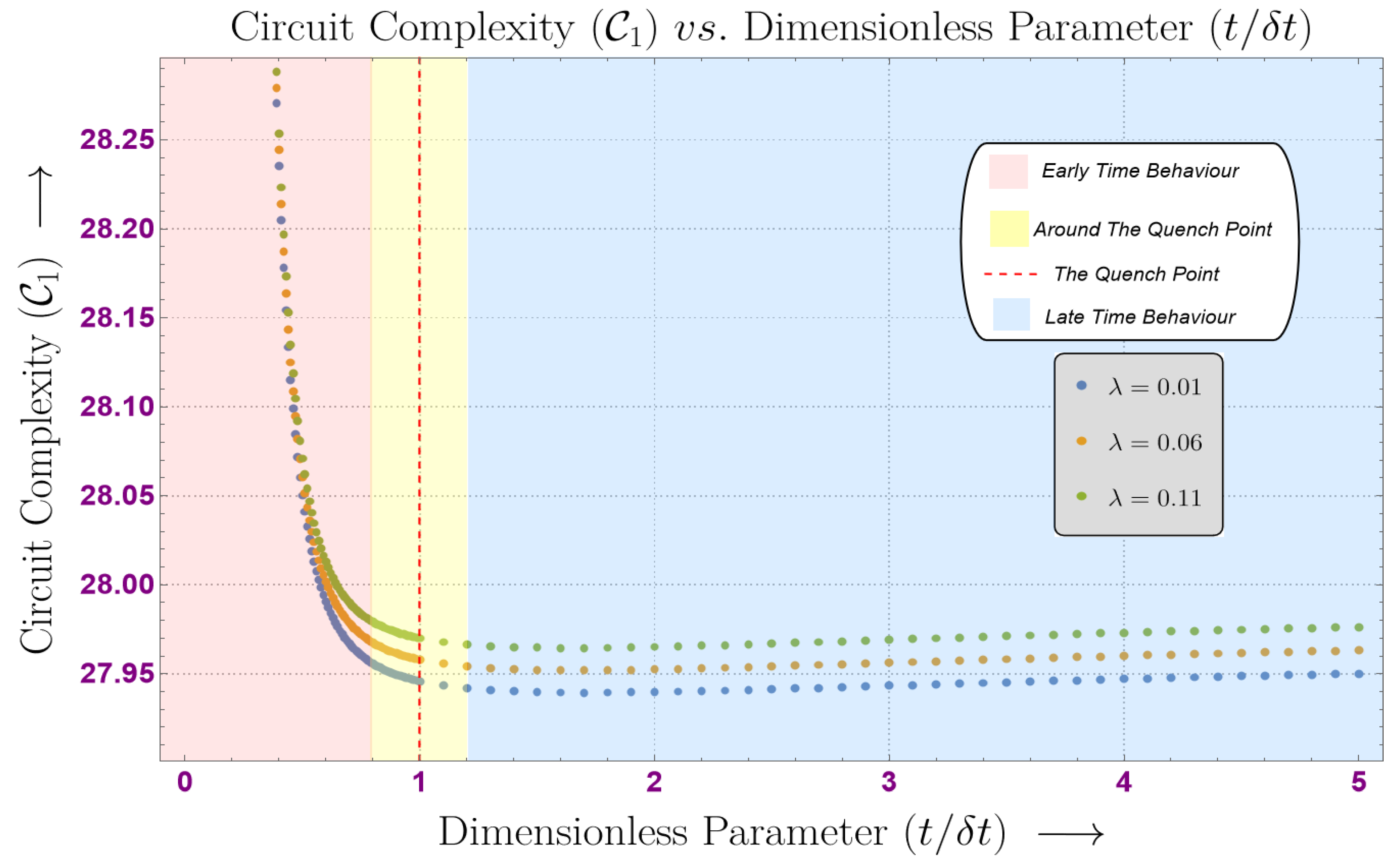
• The exact analytical form for the unambiguous contribution of the circuit complexity for N coupled oscillators was derived using the results of [19]. The parametric variation in this circuit complexity was then plotted with respect to the dimensionless parameter $(t/\delta t)$.
• It is evident from these plots that the unambiguous contribution of the circuit complexity decreases with respect to the dimensionless parameter. When parametrized for different quartic couplings, we find that, initially, the complexity decreases linearly following the same line, irrespective of the quartic coupling. Near to the quench point, the complexity for each quartic coupling diverges and saturates at late times. After the quench point, the complexity after divergence is clearly in direct proportion to the increasing value of the quartic coupling.
• We observed that the unambiguous contribution of the circuit complexity behaves similarly, irrespective of the number of oscillators, N. However, as N increases, the respective value of the complexity increases at any particular time. Using this, we commented on the continuum limit where the results would still be the same.
• Furthermore, it is clear that the unambiguous contribution of the circuit complexity for the chosen set of parameters is proportional to the increasing number of dimensions at early times. However, at the quench point, the unambiguous contribution of the circuit complexity attains a constant value, irrespective of the number of dimensions, and thermalizes at late times.

In conclusion, we have presented a novel approach to study the time-dependent circuit complexity in the context of quenched interacting field theory. By combining the invariant operator method and Nielsen’s geometric approach, we have derived the analytical expression for circuit complexity and explored its behavior under various parametric conditions. Our results demonstrate that the quenching of the system has a significant impact on the circuit complexity of interacting field theories. Our work provides a new perspective on the understanding of the dynamical behavior of circuit complexity in interacting field theories. It also opens up avenues for future research, such as the exploration of circuit complexity in other interacting field theories and the study of its relationship with other quantum information theoretic quantities.

Future Prospects:

• In this work, we explored the effects of quantum quenching on QFT with quartic coupling. In the future, it would be interesting to explore the effects of quantum quenching on Krylov complexity [47,48,49,50,51] for QFT with quartic coupling.
• Some of the works focusing on understanding the connection between complexity and quantum entanglement can be found in [40,52,53,54,55]. The connection between complexity and quantum entanglement in the case of quenched theories might turn out to be fruitful.

References

1. Calabrese, P.; Cardy, J. Entanglement entropy and quantum field theory. J. Stat. Mech. Theory Exp. 2004, 2004, 06002. [Google Scholar] [CrossRef] [Green Version]
2. Witten, E. Notes on Some Entanglement Properties of Quantum Field Theory. arXiv 2018, arXiv:1803.04993. [Google Scholar]
3. Nishioka, T. Entanglement entropy: Holography and renormalization group. Rev. Mod. Phys. 2018, 90, 035007. [Google Scholar] [CrossRef] [Green Version]
4. Blanco, D. Quantum information measures and their applications in quantum field theory. arXiv 2017, arXiv:1702.07384. [Google Scholar]
5. Headrick, M. Lectures on entanglement entropy in field theory and holography. arXiv 2019, arXiv:1907.08126. [Google Scholar]
6. Amico, L.; Fazio, R.; Osterloh, A.; Vedral, V. Entanglement in many-body systems. Rev. Mod. Phys. 2008, 80, 517–576. [Google Scholar] [CrossRef] [Green Version]
7. Cirac, J.I. Entanglement in many-body quantum systems. arXiv 2012, arXiv:1205.3742. [Google Scholar]
8. Susskind, L. Three Lectures on Complexity and Black Holes. arXiv 2018, arXiv:1810.11563. [Google Scholar]
9. Brown, A.R.; Susskind, L.; Zhao, Y. Quantum Complexity and Negative Curvature. Phys. Rev. D 2017, 95, 045010. [Google Scholar] [CrossRef] [Green Version]
10. Brown, A.R.; Roberts, D.A.; Susskind, L.; Swingle, B.; Zhao, Y. Holographic Complexity Equals Bulk Action? Phys. Rev. Lett. 2016, 116, 191301. [Google Scholar] [CrossRef] [Green Version]
11. Brown, A.R.; Roberts, D.A.; Susskind, L.; Swingle, B.; Zhao, Y. Complexity, action, and black holes. Phys. Rev. D 2016, 93, 086006. [Google Scholar] [CrossRef] [Green Version]
12. Susskind, L. Entanglement is not enough. Fortsch. Phys. 2016, 64, 49–71. [Google Scholar] [CrossRef] [Green Version]
13. Susskind, L.; Zhao, Y. Switchbacks and the Bridge to Nowhere. arXiv 2014, arXiv:1408.2823. [Google Scholar]
14. Stanford, D.; Susskind, L. Complexity and Shock Wave Geometries. Phys. Rev. D 2014, 90, 126007. [Google Scholar] [CrossRef] [Green Version]
15. Susskind, L. Computational Complexity and Black Hole Horizons. Fortsch. Phys. 2016, 64, 24–43. [Google Scholar] [CrossRef] [Green Version]
16. Jefferson, R.; Myers, R.C. Circuit complexity in quantum field theory. J. High Energy Phys. 2017, 10, 107. [Google Scholar] [CrossRef] [Green Version]
17. Hackl, L.; Myers, R.C. Circuit complexity for free fermions. J. High Energy Phys. 2018, 7, 139. [Google Scholar] [CrossRef] [Green Version]
18. Chapman, S.; Heller, M.P.; Marrochio, H.; Pastawski, F. Toward a Definition of Complexity for Quantum Field Theory States. Phys. Rev. Lett. 2018, 120, 121602. [Google Scholar] [CrossRef] [Green Version]
19. Bhattacharyya, A.; Shekar, A.; Sinha, A. Circuit complexity in interacting QFTs and RG flows. J. High Energy Phys. 2018, 10, 140. [Google Scholar] [CrossRef] [Green Version]
20. Polkovnikov, A.; Sengupta, K.; Silva, A.; Vengalattore, M. Colloquium: Nonequilibrium dynamics of closed interacting quantum systems. Rev. Mod. Phys. 2011, 83, 863–883. [Google Scholar] [CrossRef] [Green Version]
21. Gogolin, C.; Eisert, J. Equilibration, thermalisation, and the emergence of statistical mechanics in closed quantum systems. Rep. Prog. Phys. 2016, 79, 056001. [Google Scholar] [CrossRef] [PubMed] [Green Version]
22. Calabrese, P.; Essler, F.H.L.; Mussardo, G. Introduction to ‘quantum integrability in out of equilibrium systems’. J. Stat. Mech. Theory Exp. 2016, 2016, 064001. [Google Scholar] [CrossRef]
23. Calabrese, P.; Cardy, J. Quantum Quenches in Extended Systems. J. Stat. Mech. 2007, 706, P06008. [Google Scholar] [CrossRef] [Green Version]
24. Basu, P.; Das, S.R. Quantum Quench across a Holographic Critical Point. J. High Energy Phys. 2012, 1, 103. [Google Scholar] [CrossRef] [Green Version]
25. Buchel, A.; Lehner, L.; Myers, R.C.; van Niekerk, A. Quantum quenches of holographic plasmas. J. High Energy Phys. 2013, 5, 067. [Google Scholar] [CrossRef] [Green Version]
26. Das, S.R.; Galante, D.A.; Myers, R.C. Universal scaling in fast quantum quenches in conformal field theories. Phys. Rev. Lett. 2014, 112, 171601. [Google Scholar] [CrossRef] [PubMed] [Green Version]
27. Das, S.R.; Galante, D.A.; Myers, R.C. Universality in fast quantum quenches. J. High Energy Phys. 2015, 2, 167. [Google Scholar] [CrossRef]
28. Das, S.R.; Galante, D.A.; Myers, R.C. Smooth and fast versus instantaneous quenches in quantum field theory. J. High Energy Phys. 2015, 8, 073. [Google Scholar] [CrossRef]
29. Das, S.R.; Galante, D.A.; Myers, R.C. Quantum Quenches in Free Field Theory: Universal Scaling at Any Rate. J. High Energy Phys. 2016, 5, 164. [Google Scholar] [CrossRef] [Green Version]
30. Alba, V.; Calabrese, P. Entanglement dynamics after quantum quenches in generic integrable systems. SciPost Phys. 2018, 4, 017. [Google Scholar] [CrossRef]
31. Ghosh, S.; Gupta, K.S.; Srivastava, S.C.L. Entanglement dynamics following a sudden quench: An exact solution. Europhys. Lett. 2017, 120, 50005. [Google Scholar] [CrossRef] [Green Version]
32. Ghosh, S.; Gupta, K.S.; Srivastava, S.C.L. Exact relaxation dynamics and quantum information scrambling in multiply quenched harmonic chains. Phys. Rev. E 2019, 100, 012215. [Google Scholar] [CrossRef] [Green Version]
33. Camargo, H.A.; Caputa, P.; Das, D.; Heller, M.P.; Jefferson, R. Complexity as a Novel Probe of Quantum Quenches: Universal Scalings and Purifications. Phys. Rev. Lett. 2019, 122, 081601. [Google Scholar] [CrossRef] [PubMed] [Green Version]
34. Alves, D.W.F.; Camilo, G. Evolution of complexity following a quantum quench in free field theory. J. High Energy Phys. 2018, 2018, 29. [Google Scholar] [CrossRef] [Green Version]
35. Lewis, H.R.; Riesenfeld, W.B. An exact quantum theory of the time-dependent harmonic oscillator and of a charged particle in a time-dependent electromagnetic field. J. Math. Phys. 1969, 10, 1458–1473. [Google Scholar] [CrossRef]
36. Adiabatic evolution under quantum control. Ann. Phys. 2012, 327, 1293–1303. [CrossRef] [Green Version]
37. Ye, M.-Y.; Zhou, X.-F.; Zhang, Y.-S.; Guo, G.-C. Two kinds of quantum adiabatic approximation. Phys. Lett. A 2007, 368, 18–24. [Google Scholar] [CrossRef] [Green Version]
38. Choi, J.R. Perturbation theory for time-dependent quantum systems involving complex potentials. Front. Phys. 2020, 8, 189. [Google Scholar] [CrossRef]
39. Choudhury, S.; Gharat, R.M.; Mandal, S.; Pandey, N.; Roy, A.; Sarker, P. Entanglement in interacting quenched two-body coupled oscillator system. Phys. Rev. D 2022, 106, 025002. [Google Scholar] [CrossRef]
40. Caputa, P.; Das, S.R.; Nozaki, M.; Tomiya, A. Quantum Quench and Scaling of Entanglement Entropy. Phys. Lett. B 2017, 772, 53–57. [Google Scholar] [CrossRef]
41. Nielsen, M.A. A geometric approach to quantum circuit lower bounds. arXiv 2005, arXiv:0502070. [Google Scholar] [CrossRef]
42. Nielsen, M.A. Quantum computation as geometry. Science 2006, 311, 1133–1135. [Google Scholar] [CrossRef] [Green Version]
43. Dowling, M.R.; Nielsen, M.A. The geometry of quantum computation. Quantum Info. Comput. 2008, 8, 861–899. [Google Scholar] [CrossRef]
44. Nielsen, M.A.; Dowling, M.R.; Gu, M.; Doherty, A.C. Optimal control, geometry, and quantum computing. Phys. Rev. A 2006, 73, 062323. [Google Scholar] [CrossRef] [Green Version]
45. Yeon, K.H.; Kim, H.J.; Um, C.I.; George, T.F.; Pandey, L.N. Wave function in the invariant representation and squeezed-state function of the time-dependent harmonic oscillator. Phys. Rev. A 1994, 50, 1035–1039. [Google Scholar] [CrossRef]
46. Adhikari, K.; Choudhury, S.; Kumar, S.; Mandal, S.; Pandey, N.; Roy, A.; Sarkar, S.; Sarker, P.; Shariff, S.S. Circuit Complexity in Z2EEFT. Symmetry 2023, 15, 31. [Google Scholar] [CrossRef]
47. Parker, D.E.; Cao, X.; Avdoshkin, A.; Scaffidi, T.; Altman, E. A Universal Operator Growth Hypothesis. Phys. Rev. X 2019, 9, 041017. [Google Scholar] [CrossRef] [Green Version]
48. Caputa, P.; Liu, S. Quantum complexity and topological phases of matter. arXiv 2022, arXiv:2205.05688. [Google Scholar] [CrossRef]
49. Caputa, P.; Magan, J.M.; Patramanis, D. Geometry of Krylov complexity. Phys. Rev. Res. 2022, 4, 013041. [Google Scholar] [CrossRef]
50. Adhikari, K.; Choudhury, S.; Roy, A. Krylov Complexity in Quantum Field Theory. arXiv 2022, arXiv:2204.02250. [Google Scholar]
51. Adhikari, K.; Choudhury, S. Cosmological Krylov Complexity. arXiv 2022, arXiv:2203.14330. [Google Scholar]
52. Adhikari, K.; Choudhury, S.; Chowdhury, S.; Shirish, K.; Swain, A. Circuit complexity as a novel probe of quantum entanglement: A study with black hole gas in arbitrary dimensions. Phys. Rev. D 2021, 104, 065002. [Google Scholar] [CrossRef]
53. Choudhury, S.; Chowdhury, S.; Gupta, N.; Mishara, A.; Selvam, S.P.; Panda, S.; Pasquino, G.D.; Singha, C.; Swain, A. Circuit Complexity from Cosmological Islands. Symmetry 2021, 13, 1301. [Google Scholar] [CrossRef]
54. Eisert, J. Entangling Power and Quantum Circuit Complexity. Phys. Rev. Lett. 2021, 127, 020501. [Google Scholar] [CrossRef]
55. Mathur, S.D. Three puzzles in cosmology. Int. J. Mod. Phys. D 2020, 29, 2030013. [Google Scholar] [CrossRef]
56. Holzhey, C.; Larsen, F.; Wilczek, F. Geometric and renormalized entropy in conformal field theory. Nucl. Phys. B 1994, 424, 443–467. [Google Scholar] [CrossRef] [Green Version]
57. Mukherjee, S.; Choudhury, A.; Guha, P. Generalized damped Milne-Pinney equation and Chiellini method. arXiv 2016, arXiv:1603.08747. [Google Scholar]
Figure 1. Log–log variation of the total circuit complexity (C) with respect to the quench rate ( δ t ) for different orders of the coupling constant, λ , for two coupled oscillators with quartic perturbation.
Symmetry 15 00655 g001
Figure 2. Variation in the circuit complexity for the A 1 block ( C 1 ) for N = 10 , with respect to the dimensionless parameter ( t / δ t ) for different orders of the coupling constant λ .
Symmetry 15 00655 g002
Figure 3. Semi-Log variation in the circuit complexity for the A 1 block ( C 1 ) at λ = 0.01 , with respect to the dimensionless parameter ( t / δ t ) for different values of N.
Symmetry 15 00655 g003
Figure 4. Semi-Log variation in the circuit complexity for the A 1 block ( C 1 ) at λ = 0.01 , N = 10 , with respect to the dimensionless parameter ( t / δ t ) for different dimensions d.
Symmetry 15 00655 g004
Disclaimer/Publisher’s Note: The statements, opinions and data contained in all publications are solely those of the individual author(s) and contributor(s) and not of MDPI and/or the editor(s). MDPI and/or the editor(s) disclaim responsibility for any injury to people or property resulting from any ideas, methods, instructions or products referred to in the content.