The Impact of Heat Source and Temperature Gradient on Brinkman–Bènard Triple-Diffusive Magneto-Marangoni Convection in a Two-Layer System

Abstract

The effect of a heat source and temperature gradient on Brinkman–Bènard Triple-Diffusive magneto-Marangoni (BBTDMM) convection in a two-layer system is investigated. The two-layer system is horizontally infinite and is surrounded on all sides by adiabatic boundaries. It is exposed to basic uniform and non-uniform temperature profiles and heat sources. The appropriate eigenvalues and thermal Marangoni numbers (TMNs), which depend on temperature and concentration, are obtained for the temperature profiles (TPs) for lower rigid and higher free boundaries with surface tension. The transformed system of ordinary differential equations is solved by using an exact technique. For all three TPs, the impact of significant relevant parameters on these eigenvalues, and hence on BBTDMM convection, are investigated versus the thermal ratio. It is observed that, by increasing the values of the modified internal Rayleigh number for the fluid layer and the solute Marangoni numbers, the Darcy number, and the viscosity ratio for the set of physical parameters chosen in the study, one can postpone BBTDMM convection. Higher values of the modified internal Rayleigh numbers for the porous layer augment BBTDMM convection.

1. Introduction

Many academics are interested in three-component convection problems because the presence of triple-diffusive components is quite prevalent and natural in practically all real-time problems. Ravi et al. [1] demonstrated free convection between two vertical walls by considering temperature-dependent source/sink. Chung Liu et al. [2] studied the effects of a magnetic field, viscous dissipation, a nonuniform heat source and/or sink, and thermal radiation on flow and heat transfer in a hydromagnetic liquid film over an unstable stretched sheet with a prescribed heat flux condition. Srinivasacharya and Surender [3] studied a viscous fluid using a double stratification method that took into account the Soret and Dufour effects. MHD effects on heat transmission over a stretching sheet immersed in a porous medium with changing viscosity, viscous dissipation, and heat source/sink were investigated by Dessie and Kishan [4]. A Casson fluid with a non-uniform heat source/sink was considered by Gireesha et al. [5]. The characteristics of a heat source/sink in a magneto-hydrodynamic flow of a non-Newtonian fluid submerged in a porous medium were examined by Hayat et al. [6]. Mabood et al. [7] looked into micropolar fluids with non-uniform heat sources and sinks. Oni [8] offered an analytical solution for the combined influence of a heat source, porosity, and thermal radiation on mixed convection flow in a vertical annulus. According to his research, increases in the radiation and heat source parameters result in a rise in the fluid temperature and heat transfer rate. Hakeem et al. [9] conducted nonlinear research on the influence of non-uniform heat generation/absorption on the hydromagnetic flow of a nanofluid across a vertical plate. The impacts of viscous dissipation and a non-uniform heat source and sink on Casson fluid flow for an unstable, inclined, permeable, stretched surface were investigated by Raju et al. [10]. Khan et al. [11] investigated the influence of a magnetic field on the flow of a UCMF with the property of a heat source/sink immersed in a porous medium. The effects of the magnetic field and internal heat generation on three-component convection in an Oldroyd-B liquid were investigated using the Galerkin method by Gayathri et al. [12]. Archana et al. [13] studied triple-diffusive flow in the presence of a nanofluid. Rana et al. [14] used analytical methods to investigate the start of triple-diffusive linear aperiodic and periodic convection for a magnetic field-exposed closely packed rotating porous layer saturated with nanofluid. Manjunatha and Sumithra [15] studied the triple-diffusive convection for composite systems in the absence of a constant heat source. Taiwo et al. [16] used Riemann sum approximation to investigate the effect of isothermal and isoflux heating/cooling with a heat source/sink on the unsteady hydromagnetic-free convective flow of a viscous incompressible fluid in an annulus. Jha and Samaila [17] presented research on a close form of solution to MHD free convection with nanoparticles with a generated magnetic field effect. Thirupathi and Mishra [18] investigated the impact of a heat source/sink, as well as space- and temperature-dependent viscosity and Joule dissipation, on 3D magnetohydrodynamic radiating Eyring–Powell nanofluid streamline flow via a stretching sheet under convective conditions. Naveen and Singh [19] investigated Hall effects and a transverse magnetic field in the presence of a heat source and sink.

The symmetry laws serve as the foundation for theoretical and mathematical physics. They are frequently used as selection rules, making it possible to pick out of a group of mathematically valid equations that have the desired properties. Such symmetry selection can occasionally produce an original equation. We investigate the symmetry characteristics of the heat, momentum, and species equation for a convection-related problem. The impact of the heat source/sink parameter on the laminar transient free convective flow through a vertical cylinder filled with a permeable material was investigated by Anurag and Singh [20] using the Laplace transform scheme. Anurag et al. [21] examined the effect of Newtonian heating/cooling in the presence of a heat source/sink on laminar free convective flow in a vertical annular permeability zone. They discovered that in the case of Newtonian heating, velocity and temperature are increased, whereas in the case of Newtonian cooling, the opposite is true for both the source and sink. Rudziva et al. [22] investigated the three types of rotational modulations in salted water triple-diffusive convection. Pranesh et al. [23] used linear and non-linear techniques to investigate three-component convection in a Newtonian fluid. A regular perturbation method is used in linear theory to obtain the equations for the Rayleigh number and the corrected Rayleigh number. Nagendramma et al. [24] use Lie-group transformation to examine the dynamics of triple-diffusive convection. They discovered that as the Lewis number rises, the impact of the heat and mass transfer rates declined for both fluid flow instances. Investigation of mixed convection under the influence of MHD, velocity slip, and heat source/sink was conducted by Zainodin et al. [25]. The importance of radiation and Soret and Dufour’s impacts for MHD flow regarding slip, temperature, and concentration were all examined by Lakshmi Devi et al. [26]. The Soret and Dufour effects, heat generation, heat radiation, and chemical reactions in a Casson fluid were all investigated by Kune et al. [27]. Different effects on an Oldroyd-B bio-nanofluid inside a confined channel were observed by Kaleem et al. [28]. Khan et al. [29] investigated stability analysis with a heat source present. Khan et al. [30] investigated the effects of an inclined magnetic field and double-diffusive convection in nanofluids. With an internal heat source modelled by Darcy’s law, Rafeek et al. [31] investigated the effects of throughflow and the Coriolis force on the beginning of double-diffusive convection. Corcione and Quintino [32] explored the numerical analysis of Rayleigh–Benard convection in nanofluids. Using single-mode equations, Liu and Knobloch [33] investigated convection and double-diffusive convection in a porous medium. Manjunatha and Sumithra [34] and Manjunatha et al. [35] examined the single- and double-diffusive convection for composite layer systems using an exact technique. They found that an inverted parabolic profile is more stable and stabilises the system.

According to the papers cited above, several investigations on magneto-convection in a single, double, or porous layer in the presence of a heat source have indeed been conducted. However, the reality of constant heat sources and sinks and uneven temperature gradients is one that is rarely addressed. In this work, the impacts of a continuous heat source/sink and an applied magnetic field as well as those of temperature gradients (linear, parabolic, and inverted parabolic profiles) on triple-diffusive natural convection are researched using a two-layer structure. The eigenvalue problem has been solved utilising an exact approach while accounting for the heat source using the Darcy–Brinkman model. It has been found that one can delay BBTDMM convection by raising the values for the set of physical parameters selected for the investigation. BBTDMM convection is enhanced by higher values of the modified internal Rayleigh numbers for the porous layer. This research will undoubtedly be useful in a variety of applications in engineering, geophysics, climatology, and astronomy.

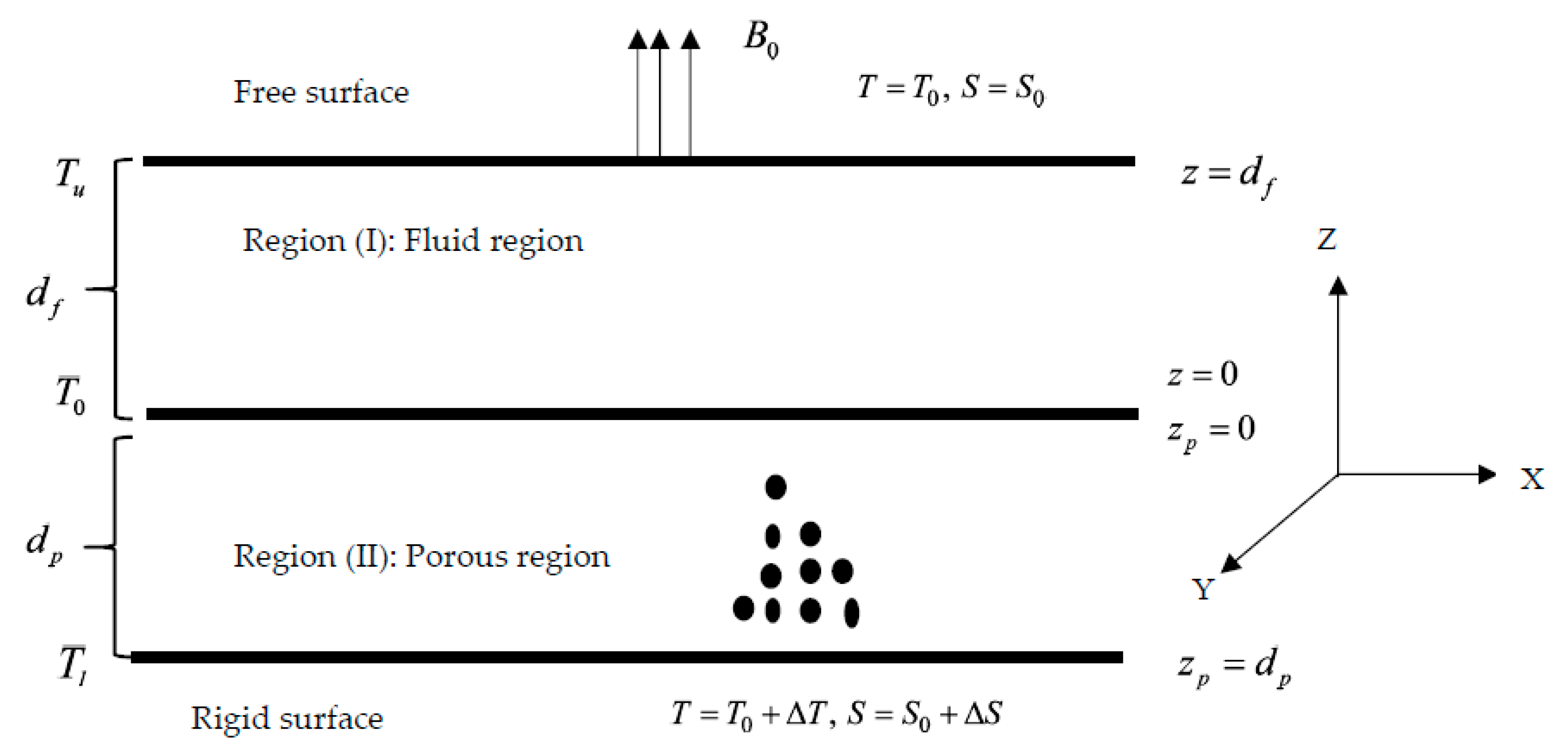
2. Formulation of the Problem and Physical Model

Consider a horizontally infinite, electrically conducting, fluid-saturated, isotropic, incompressible, sparsely packed three-component fluid layer of thickness d_f underlying a porous layer of thickness $d_p$ with a vertical Z-direction-imposed magnetic field of intensity $B_0$ and constant heat sources ${\Phi }_f$ and ${\Phi }_p$. The porous layer’s lower surface is rigid, while the fluid layer’s upper surface is free, with surface tension effects depending on temperature and concentration. The interface between the fluid and saturated porous medium is at $z=0=z_p$; the temperature and concentration differences between the lower and upper bounds are denoted $\Delta T\&\Delta C$, respectively. Also, $T_0,C_0$ are the initial temperature and concentration respectively. As shown in Figure 1, a Cartesian coordinate system is used, with the origin at the interface between the fluid layer (region I) and porous layer (region II) and the Z-axis running vertically upwards. The following model takes the relevant equations with an Oberbeck–Boussinesq approximation (refer to Barna and Matyas [36], Barna et al. [37], and Shivakumara et al. [38,39]).

Fluid layer: region I

$$\nabla .{\overrightarrow{V}}_f=0$$

(1)

$$\nabla .\overrightarrow{B}=0$$

(2)

$${\rho }_0\left(\frac{\partial {\overrightarrow{V}}_f}{\partial t}+({\overrightarrow{V}}_f.\nabla ){\overrightarrow{V}}_f\right)=-\nabla P_f+{\mu }_f{\nabla }^2{\overrightarrow{V}}_f+{\gamma }_f(\overrightarrow{B}.\nabla )\overrightarrow{B}$$

(3)

$$\frac{\partial T_f}{\partial t}+({\overrightarrow{V}}_f.\nabla )T_f={\kappa }_f{\nabla }^2{T}_f+{\Phi }_f$$

(4)

$$\frac{\partial S_1}{\partial t}+({\overrightarrow{V}}_f.\nabla )S_1={\kappa }_{f1}{\nabla }^2{S}_{f1}$$

(5)

$$\frac{\partial S_2}{\partial t}+({\overrightarrow{V}}_f.\nabla )S_2={\kappa }_{f2}{\nabla }^2{S}_{f2}$$

(6)

$$\frac{\partial \overrightarrow{B}}{\partial t}=\nabla \times {\overrightarrow{V}}_f\times \overrightarrow{B}+{\nu }_f{\nabla }^2\overrightarrow{B}$$

(7)

The relevant equations for the porous layer: region II

$${\nabla }_p.\overrightarrow{V_p}=0$$

(8)

$${\nabla }_p.\overrightarrow{B}=0$$

(9)

$${\rho }_0\left({\varphi }^{-1}\frac{\partial \overrightarrow{V_p}}{\partial t}+{\varphi }^{-2}(\overrightarrow{V_p}.{\nabla }_p)\overrightarrow{V_p}\right)=-{\nabla }_p{P}_p-\frac{{\mu }_p}{K}\overrightarrow{V_p}+{\mu }_p{\nabla }_p^2\overrightarrow{V_p}+{\gamma }_p(\overrightarrow{B}.{\nabla }_p)\overrightarrow{B}$$

(10)

$$M\frac{\partial T_p}{\partial t}+(\overrightarrow{V_p}.{\nabla }_p)T_p={\kappa }_p{\nabla }_p^2{T}_p+{\Phi }_p$$

(11)

$$\varphi \frac{\partial S_{p1}}{\partial t}+(\overrightarrow{V_p}.{\nabla }_p)S_{p1}={\kappa }_{p1}{\nabla }_p^2{S}_{p1}$$

(12)

$$\varphi \frac{\partial S_{p2}}{\partial t}+(\overrightarrow{V_p}.{\nabla }_p)S_{p2}={\kappa }_{p2}{\nabla }_p^2{S}_{p2}$$

(13)

$$\varphi \frac{\partial \overrightarrow{B}}{\partial t}={\nabla }_p\times \overrightarrow{V_p}\times \overrightarrow{B}+{\nu }_p{\nabla }_p^2\overrightarrow{B}$$

(14)

where $‘f’$ denotes the fluid layer (region I), ${\overrightarrow{V}}_f$ is the velocity vector, ${\rho }_0$ is the fluid density, ${\mu }_f$ is the fluid viscosity, $P_f$ is the total hydromagnetic pressure, $\overrightarrow{B}$ is the magnetic field, $T_f$ is the temperature, ${\kappa }_f$ is the thermal diffusivity of the fluid, ${\nu }_f$ is the magnetic viscosity, ${\gamma }_f$ is the magnetic permeability, ${\kappa }_{f1},{\kappa }_{f2}$ are the solute diffusivities of the fluid, $S_{f1},S_{f2}$ are salinity field1 and salinity field2, respectively, the subscript ‘p’ denotes the quantities in region II, $\varphi$ is the porosity, ${\mu }_p$ is the effective viscosity of the fluid in region II, $K$ is the permeability, and $M$ is the heat capacity ratio.

The initial state is described as follows:

Region I:

$$\begin{array}{l}{\overrightarrow{V}}_f=(0,0,0),P_f=P_{fb}(z),T_f=T_{fb}(z),S_{f1}=S_{f1b}(z),S_{f2}=S_{f2b}(z),\overrightarrow{B}=B_0(z),\\ \frac{-d_f}{\Delta T_f}\frac{d{T}_{fb}}{d{z}_f}={\chi }_f(z)\end{array}\}$$

(15)

Region II:

$$\begin{array}{l}{\overrightarrow{V}}_p=(0,0,0),P_p=P_{pb}(z_p),T_p=T_{pb}(z_p),S_{p1}=S_{1pb}(z_p),S_{p2}=S_{p2b}(z_p),\overrightarrow{B}=B_0(z_p),\\ \frac{-d_p}{\Delta T_p}\frac{d{T}_{pb}}{d{z}_p}={\chi }_p(z_p)\end{array}\}$$

(16)

The temperature and species concentration distributions $T_{fb}(z),T_{pb}(z_p)$ and $S_{fib}(z),S_{pib}(z_p)$, respectively, take the forms:

$$T_{fb}=\frac{{\Phi }_{f}z(d_f-z)}{2{\kappa }_f}+\frac{(T_u-T_0){\chi }_f(z)}{d_f}+T_{0}0\le z\le d_f$$

(17)

$$T_{pb}=\frac{-{\Phi }_p{z}_p(z_p+d_p)}{2{\kappa }_p}+\frac{(T_0-T_l){\chi }_p(z_p)}{d_p}+T_0{d}_p\le z_p\le 0$$

(18)

$$S_{fib}(z)=S_{i0}+\frac{(S_{iu}-S_{i0})z}{d_f},i=1,20\le z\le d_f$$

(19)

$$S_{pib}(z_m)=S_{i0}+\frac{(S_{i0}-S_{il})z_p}{d_p},i=1,2d_p\le z_p\le 0$$

(20)

where the basic state is represented by the subscript $‘b’$, ${\displaystyle \underset{0}{\overset{d_f}{\int }}{\chi }_f(z)}dz=1$ is the temperature profile in the fluid layer, and ${\displaystyle \underset{0}{\overset{d_p}{\int }}{\chi }_p(z_p)}d{z}_p=1$ is the same quantity in the porous layer; $T_0=\frac{{\kappa }_f{d}_p{T}_u+{\kappa }_p{d}_f{T}_l}{\kappa d_p+{\kappa }_p{d}_f}+\frac{d_f{d}_p({\Phi }_p{d}_p+{\Phi }_f{d}_f)}{2({\kappa }_f{d}_p+{\kappa }_p{d}_f)}$ and $S_{i0}=\frac{{\kappa }_{fi}{d}_p{S}_{iu}+{\kappa }_{pi}{d}_f{S}_{il}}{{\kappa }_{fi}{d}_p+{\kappa }_{pi}{d}_f},i=1,2$.

In regions I and II infinite perturbations are introduced to probe the stability of the fundamental state.

$$\begin{array}{l}{\overrightarrow{V}}_f=0+{{\overrightarrow{V}}_f}^{\prime },P_f=P_b(z)+P_f^{\prime },T_f=T_{fb}(z)+T_f^{\prime },\\ S_{f1}=S_{f1b}(z)+S_{f1}^{\prime },S_{f2}=S_{f2b}(z)+S_{f2}^{\prime },\overrightarrow{B}={\overrightarrow{B}}_0(z)+{\overrightarrow{B}}^{\prime }\end{array}\}$$

(21)

$$\begin{array}{l}{\overrightarrow{V}}_p=0+{{\overrightarrow{V}}_p}^{\prime },P_p=P_b(z)+P_p^{\prime },T_p=T_{pb}(z_p)+T_p^{\prime },\\ S_{p1}=S_{p1b}(z_p)+S_{p1}^{\prime },S_{p2}=S_{p2b}(z_p)+S_{p2}^{\prime },\overrightarrow{B}={\overrightarrow{B}}_0(z_p)+{\overrightarrow{B}}^{\prime }\end{array}\}$$

(22)

where ${{\overrightarrow{V}}_f}^{\prime }$, $P_f^{\prime },T_f^{\prime },S_{f1}^{\prime }$, $S_{f2}^{\prime }$, and ${\overrightarrow{B}}^{\prime }$, and ${{\overrightarrow{V}}_p}^{\prime }$, $P_p^{\prime },T_p^{\prime },S_{p1}^{\prime }$, $S_{p2}^{\prime }$, and ${\overrightarrow{B}}^{\prime }$ are the perturbed velocity, pressure, temperature, salinity1, salinity2, and magnetic field in regions I and II, respectively. The variables are nondimensionalized for regions I and II, respectively using $d_f,$ $d_f^2/{\kappa }_f,$${\kappa }_f/d_f,$$T_0-T_u,$$S_{10}-S_{1u},$$S_{20}-S_{2u}$, $B_0$ and $d_p,d_p^2/{\kappa }_p,{\kappa }_p/d_p,$$T_l-T_0,S_{1l}-S_{10},$ $S_{2l}-S_{20},B_0$.

3. Normal Mode Technique and Stability Analysis

The solutions for dependent variables are established in regions I and II as follows:

$$\left(w,T_f,S_{f1},S_{f2},\overrightarrow{B}\right)=\left(W_f(z),{\Theta }_f(z),{\Sigma }_{f1}(z),{\Sigma }_{f2}(z),\overrightarrow{B}(z)\right)exp\left(ilx+imy+n_{f}t\right)$$

(23)

$$\left(w,T_p,S_{p1},S_{p2},\overrightarrow{B}\right)=\left(W_p(z_p),{\Theta }_p(z_p),{\Sigma }_{p1}(z_p),{\Sigma }_{p2}(z_p),\overrightarrow{B}(z_p)\right)exp\left(i{l}_{p}x+i{m}_{p}y+n_p{t}_p\right)$$

(24)

where $l,m$ and $l_p,m_p$ are wave numbers in the $x$ and $y$ direction, respectively, and $n_f,n_p$ are growth rates in the fluid and porous layer respectively.

By applying Equations (15), (16) and (21)–(24), as well as Equations (1)–(14), using normal mode analysis and assuming that the notion of stability exchange is applicable for the current situation (see Manjunatha and Sumithra [15]):

Fluid layer: Region I $0\le z\le 1$

$$\left[{(D_f^2-a_f^2)}^2-Q_f{D}_f^2\right]W_f(z)=0$$

(25)

$$(D_f^2-a_f^2){\Theta }_f(z)=-\left[{\chi }_f(z)+R_a^{*}(2z-1)\right]W_f(z)$$

(26)

$${\tau }_{f1}(D_f^2-a_f^2){\Sigma }_{f1}(z)=-W_f(z)$$

(27)

$${\tau }_{f2}(D_f^2-a_f^2){\Sigma }_{f2}(z)=-W_f(z)$$

(28)

Porous layer: Region II $1\le z_p\le 0$

$$[(D_p^2-a_p^2)\widehat{\mu }{\beta }^2-1](D_p^2-a_p^2)W_p(z_p)=Q_p{\beta }^2{D}_p^2{W}_p(z_p)$$

(29)

$$(D_p^2-a_p^2){\Theta }_p(z_p)=-\left[{\chi }_p(z_p)+R_{ap}^{*}(2z_p+1)\right]W_p(z_p)$$

(30)

$${\tau }_{p1}(D_p^2-a_p^2){\Sigma }_{p1}(z_p)=-W_p(z_p)$$

(31)

$${\tau }_{p2}(D_p^2-a_p^2){\Sigma }_{p2}(z_p)=-W_p(z_p)$$

(32)

where $D_f=\frac{d}{dz}$, $a_f=\sqrt{l^2+m^2}$ is the resultant wave number, $Q_f$ is the Chandrasekhar number,$R_a^{*}=\frac{R_{If}}{2(T_0-T_u)}$ is the modified internal Rayleigh number (MRN), $R_{If}=\frac{{\Phi }_f{d}_f^2}{{\kappa }_f}$ is the internal Rayleigh number, $W_f(z)$ is the vertical velocity, ${\Theta }_f(z)$ is the temperature distribution, ${\tau }_{f1}=\frac{{\kappa }_{f1}}{{\kappa }_f}$ and ${\tau }_{f2}=\frac{{\kappa }_{f2}}{{\kappa }_f}$ are the diffusivity ratios, ${\Sigma }_{f1}(z),{\Sigma }_{f2}(z)$ are the salinity distributions in region I, and $D_p=\frac{d}{d{z}_p}$, $a_p=\sqrt{l_p^2+m_p^2}$, $Q_p$, $R_{ap}^{*}=\frac{R_{Ip}}{2(T_l-T_0)}$, $R_{Ip}=\frac{{\Phi }_p{d}_p^2}{{\kappa }_p}$, $W_p(z_p),{\Theta }_p(z_p)$, ${\tau }_{p1}=\frac{{\kappa }_{p1}}{{\kappa }_p}$, ${\tau }_{p2}=\frac{{\kappa }_{p2}}{{\kappa }_p}$, and ${\Sigma }_{p1}(z_p),{\Sigma }_{p2}(z_p)$ are similar quantities in the porous layer. Because the composite layers’ horizontal wave numbers must match, so that we have $a_p=a_f\widehat{d}$, here, $\widehat{d}=\frac{d_p}{d_f}$ is the depth ratio.

Before being expanded in normal mode, all of the boundary conditions are nondimensionalized (see Manjunatha and Sumithra [15]).

The velocity, thermal, and salinities boundary conditions are respectively:

$$\begin{array}{l}{W}_f(1)=0,W_p(1)=0,D_p{W}_p(1)=0,\widehat{T}{W}_f(0)=W_p(0),\widehat{T}\widehat{d^2}(D_f^2+a_f^2)W_f(0)=\widehat{\mu }(D_p^2+a_p^2)W_p(0),\\ \widehat{T}\widehat{d}{D}_f{W}_f(0)=D_p{W}_p(0),\widehat{T}\widehat{d^3}{\beta }^2[(D_f^3-3a_f^2{D}_f)]W_f(0)=[-D_p+\widehat{\mu }{\beta }^2(D_p^3-3a_p^2{D}_p)]W_p(0)\end{array}\}$$

(33)

$$D_f{\Theta }_f(1)=0,{\Theta }_f(0)=\widehat{T}{\Theta }_p(0),D_f{\Theta }_f(0)=D_p{\Theta }_p(0),D_p{\Theta }_p(1)=0$$

(34)

$$D_f{\Sigma }_{f1}(1)=0,{\Sigma }_{f1}(0)={\widehat{S}}_1{\Sigma }_{p1}(0),D_f{\Sigma }_{f1}(0)=D_p{\Sigma }_{p1}(0),D_p{\Sigma }_{p1}(1)=0$$

(35)

$$D_f{\Sigma }_{f2}(1)=0,{\Sigma }_{f2}(0)={\widehat{S}}_2{\Sigma }_{p2}(0),D_f{\Sigma }_{f2}(0)=D_p{\Sigma }_{p2}(0),D_p{\Sigma }_{p2}(1)=0$$

(36)

where $\widehat{T}$ is the thermal ratio, $\widehat{\mu }=\frac{{\mu }_p}{{\mu }_f}$ is the viscosity ratio, ${\widehat{S}}_i=\frac{S_{il}-S_{i0}}{S_{i0}-S_{iu}},i=1,2$ is the solute diffusivity ratio, and ${\beta }^2=\frac{K}{d_p^2}=Da$ is the porous parameter.

4. Profiles and Thermal Marangoni Numbers

The thermal Marangoni numbers are obtained analytically for linear, parabolic, and inverted parabolic profiles using an exact technique.

4.1. Velocity Profiles

By utilizing the conditions of Equation (33), the velocity profiles are derived by solving Equations (25) and (29) as follows

$$W_f(z)=A_1[\cosh ({\delta }_{f}z)+a_1\sinh ({\delta }_{f}z)+a_2\cosh ({\zeta }_{f}z)+a_3\sinh ({\zeta }_{f}z)]$$

(37)

$$W_p(z_p)=A_1[a_4\cosh ({\eta }_p{z}_p)+a_5\sinh ({\eta }_p{z}_p)+a_6\cosh ({\psi }_p{z}_p)+a_7(\sinh {\psi }_p{z}_p)]$$

(38)

where

$$\begin{array}{c}{\delta }_f=\frac{\sqrt{Q_f}+\sqrt{Q_f+4a_f^2}}{2},{\zeta }_f=\frac{\sqrt{Q_f}-\sqrt{Q_f+4a_f^2}}{2},\\ {\eta }_p^2=\frac{r_1+\sqrt{r_1^2-4r_2}}{2},{\psi }_p^2=\frac{r_1-\sqrt{r_1^2-4r_2}}{2},r_1=\frac{(2\widehat{\mu }{\beta }^2{a}_p^2+1+Q_p{\beta }^2)}{\widehat{\mu }{\beta }^2},r_2=\frac{(a_p^2+a_p^4\widehat{\mu }{\beta }^2)}{\widehat{\mu }{\beta }^2},\\ a_1=\frac{1}{{\delta }_{14}}(a_6{\delta }_{15}+a_7{\delta }_{16}+{\delta }_{17}),a_2=a_6{\delta }_5+{\delta }_6,a_3=\frac{1}{{\delta }_9}(a_1{\delta }_{10}+a_7{\delta }_{11}),\\ a_4={\delta }_7+a_6{\delta }_8,a_5=a_1{\delta }_{12}+a_7{\delta }_{13},a_6=\frac{{\delta }_{23}{\delta }_{25}-{\delta }_{26}{\delta }_{22}}{{\delta }_{25}{\delta }_{21}-{\delta }_{24}{\delta }_{22}},\\ a_7=\frac{{\delta }_{23}{\delta }_{24}-{\delta }_{26}{\delta }_{21}}{{\delta }_{24}{\delta }_{22}-{\delta }_{25}{\delta }_{21}},{\delta }_1=\widehat{T}{\beta }^2\widehat{d^3}({\delta }_f^3-3a_f^2{\delta }_f),{\delta }_2=\widehat{T}{\beta }^2\widehat{d^3}({\zeta }_f^3-3a_f^2{\zeta }_f),\\ {\delta }_3=\widehat{\mu }{\beta }^2({\eta }_p^3-3a_p^2{\eta }_p)-{\eta }_p,{\delta }_4=\widehat{\mu }{\beta }^2({\psi }_p^3-3a_p^2{\psi }_p)-{\psi }_p,{\delta }_5=\frac{\widehat{\mu }[({\psi }_p^2+a_p^2)-\widehat{T}({\eta }_p^2+a_p^2)]}{\widehat{T}\widehat{d^2}({\zeta }_f^2+a_f^2)-\widehat{\mu }\widehat{T}({\eta }_p^2+a_p^2)},\\ {\delta }_6=\frac{\widehat{\mu }({\eta }_p^2+a_p^2)-\widehat{d^2}({\delta }_f^2+a_f^2)}{\widehat{d^2}({\zeta }_f^2+a_f^2)-\widehat{\mu }({\eta }_p^2+a_p^2)},{\delta }_7=\widehat{T}(1+{\delta }_6),{\delta }_8=\widehat{T}{\delta }_5-1,{\delta }_9=\frac{\widehat{T}\widehat{d}{\zeta }_f{\delta }_3-{\delta }_2{\eta }_p}{{\eta }_p},{\delta }_{10}=\frac{\widehat{T}\widehat{d}{\delta }_f{\delta }_3-{\delta }_1{\eta }_p}{{\eta }_p},\\ {\delta }_{11}=\frac{{\delta }_4{\eta }_p-{\psi }_p{\delta }_3}{{\eta }_p},{\delta }_{12}=\frac{1}{{\eta }_p{\delta }_9}\left({\delta }_9\widehat{T}\widehat{d}{\delta }_f+{\zeta }_f{\delta }_{10}\right),\\ {\delta }_{13}=\frac{1}{{\eta }_p{\delta }_9}\left(\widehat{T}\widehat{d}{\zeta }_f{\delta }_{11}-{\psi }_p{\delta }_9\right),{\delta }_{14}=\sinh {\delta }_f+\frac{{\delta }_{10}\sinh {\zeta }_f}{{\delta }_9},{\delta }_{15}={\delta }_5\cosh {\zeta }_f,\\ {\delta }_{16}=\frac{{\delta }_{11}\sinh {\zeta }_f}{{\delta }_9},{\delta }_{17}={\delta }_6\cosh {\zeta }_f+\cosh {\delta }_f,{\delta }_{18}=\frac{{\delta }_{12}{\delta }_{15}}{{\delta }_{14}},{\delta }_{19}=\frac{{\delta }_{12}{\delta }_{16}}{{\delta }_{14}}+{\delta }_{13},{\delta }_{20}=\frac{{\delta }_{12}{\delta }_{17}}{{\delta }_{14}},\\ {\delta }_{21}={\delta }_8\cosh {\eta }_p-{\delta }_{18}\sinh {\eta }_p+\cosh {\psi }_p,{\delta }_{22}=-({\delta }_{19}\sinh {\eta }_p+\sinh {\psi }_p),\\ {\delta }_{23}=\sinh {\eta }_p({\delta }_{20}-{\delta }_7\coth {\eta }_p),{\delta }_{24}=-{\eta }_p\sinh {\eta }_p({\delta }_8+{\delta }_{18}\coth {\eta }_p)-{\psi }_p\sinh {\psi }_p,\\ {\delta }_{25}=-{\eta }_p{\delta }_{19}\cosh {\eta }_p+{\psi }_p\cosh {\psi }_p,{\delta }_{26}={\delta }_{20}{\eta }_p\cosh {\eta }_p+{\delta }_7{\eta }_p\sinh {\eta }_p\end{array}$$

4.2. Salinity Profiles

We solve Equations (27) and (28) for fluid layer, (31) and (32) for porous layer salinity distributions using the salinity/concentration boundary conditions (35) and (36), as follows:

$${\Sigma }_{f1}(z)=A_1[c_{13}\cosh a_{f}z+c_{14}\sinh a_{f}z+f_1(z)]$$

(39)

$${\Sigma }_{p1}(z_p)=A_1[c_{15}\cosh a_p{z}_p+c_{16}\sinh a_p{z}_p+f_{p1}(z_p)]$$

(40)

$${\Sigma }_{f2}(z)=A_1[c_{17}\cosh a_{f}z+c_{18}\sinh a_{f}z+f_2(z)]$$

(41)

$${\Sigma }_{p2}(z_p)=A_1[c_{19}\cosh a_p{z}_p+c_{20}\sinh a_p{z}_p+f_{p2}(z_p)]$$

(42)

where

$$\begin{array}{c}{f}_1(z)=\frac{-1}{{\tau }_{f1}}\left[\frac{\cosh {\delta }_{f}z(1+a_1\tanh {\delta }_{f}z)}{{\delta }_f^2-a_f^2}+\frac{\cosh {\zeta }_{f}z(a_2+a_3\tanh {\zeta }_{f}z)}{{\zeta }_f^2-a_f^2}\right]\\ f_{p1}(z_p)=\frac{-1}{{\tau }_{p1}}\left[\frac{\cosh {\eta }_p{z}_p(a_4+a_5\tanh {\eta }_p{z}_p)}{{\eta }_p^2-a_p^2}+\frac{\cosh {\psi }_p{z}_p(a_6+a_7\tanh {\psi }_p{z}_p)}{{\psi }_p^2-a_p^2}\right]\\ f_2(z)=\frac{-1}{{\tau }_{f2}}\left[\frac{\sinh {\delta }_{f}z(\coth {\delta }_{f}z+a_1)}{{\delta }_f^2-a_f^2}+\frac{\sinh {\zeta }_{f}z(a_2\coth {\zeta }_{f}z+a_3)}{{\zeta }_f^2-a_f^2}\right]\\ f_{p2}(z_p)=\frac{-1}{{\tau }_{p2}}\left[\frac{\sinh {\eta }_p{z}_p(a_4\coth {\eta }_p{z}_p+a_5)}{{\eta }_p^2-a_p^2}+\frac{\sinh {\psi }_p{z}_p(a_6\coth {\psi }_p{z}_p+a_7)}{{\psi }_p^2-a_p^2}\right]\\ c_{13}={\widehat{S}}_1{c}_{15}+R_{100}+R_{101},c_{14}=\frac{1}{a_f}(c_{16}{a}_p+R_{102}+R_{103}),\\ c_{15}=\frac{R_{108}{a}_p\cosh a_p-R_{107}{R}_{105}}{a_p\sinh a_p(R_{107}+R_{106}\coth a_p)},c_{16}=\frac{R_{105}{R}_{106}+a_p\sinh a_p{R}_{108}}{a_p\sinh a_p(R_{107}+R_{106}{a}_p\coth a_p)}\\ c_{17}={\widehat{S}}_2{c}_{19}+R_{109}+R_{110},c_{18}=\frac{1}{a_f}(c_{20}{a}_p+R_{111}+R_{112}),\\ c_{19}=\frac{R_{117}{a}_p\cosh a_p-R_{116}{R}_{114}}{a_p\sinh a_p{R}_{116}+R_{115}{a}_p\cosh a_p},c_{20}=\frac{R_{105}{R}_{115}+a_p\sinh a_p{R}_{117}}{a_p\sinh a_p(R_{116}+R_{115}\coth a_p)},\\ R_{100}=\frac{-{\widehat{S}}_1}{{\tau }_{p1}}\left[\frac{a_4}{{\eta }_p^2-a_p^2}+\frac{a_6}{{\psi }_p^2-a_p^2}\right],R_{101}=\frac{1}{{\tau }_{f1}}\left[\frac{1}{{\delta }_f^2-a_f^2}+\frac{a_2}{{\zeta }_f^2-a_f^2}\right],\\ R_{102}=\frac{-1}{{\tau }_{p1}}\left[\frac{{\eta }_p{a}_5}{{\eta }_p^2-a_p^2}+\frac{{\psi }_p{a}_7}{{\psi }_p^2-a_p^2}\right],R_{103}=\frac{1}{{\tau }_{f1}}\left[\frac{a_1{\delta }_f}{{\delta }_f^2-a_f^2}+\frac{a_3{\zeta }_f}{{\zeta }_f^2-a_f^2}\right],\\ R_{104}=\frac{1}{{\tau }_{f1}}\left[\frac{\sinh {\delta }_f(1+a_1\coth {\delta }_f){\delta }_f}{{\delta }_f^2-a_f^2}+\frac{\sinh {\zeta }_f(a_2+a_3\coth {\zeta }_f){\zeta }_f}{{\zeta }_f^2-a_f^2}\right],\\ R_{105}=\frac{1}{{\tau }_{p1}}\left[\frac{{\eta }_p\sinh {\eta }_p(a_5\coth {\eta }_p-a_4)}{{\eta }_p^2-a_p^2}+\frac{{\psi }_p\sinh {\psi }_p(a_7\coth {\psi }_p-a_6)}{{\psi }_p^2-a_p^2}\right],\\ R_{106}={\widehat{S}}_1{a}_f\sinh a_f,R_{107}=a_p\cosh a_f,\\ R_{108}=R_{104}-(R_{100}+R_{101})a_f\sinh a_f-(R_{102}+R_{103})\cosh a_f.\\ R_{109}=\frac{-{\widehat{S}}_2}{{\tau }_{p2}}\left[\frac{a_4}{{\eta }_p^2-a_p^2}+\frac{a_6}{{\psi }_p^2-a_p^2}\right],R_{110}=\frac{1}{{\tau }_{f2}}\left[\frac{1}{{\delta }_f^2-a_f^2}+\frac{a_2}{{\zeta }_f^2-a_f^2}\right],\\ R_{111}=\frac{-1}{{\tau }_{p2}}\left[\frac{{\eta }_p{a}_5}{{\eta }_p^2-a_p^2}+\frac{{\psi }_p{a}_7}{{\psi }_p^2-a_p^2}\right],R_{112}=\frac{1}{{\tau }_{f2}}\left[\frac{a_1{\delta }_f}{{\delta }_f^2-a_f^2}+\frac{a_3{\zeta }_f}{{\zeta }_f^2-a_f^2}\right],\\ R_{113}=\frac{1}{{\tau }_{f2}}\left[\frac{(\sinh {\delta }_f+a_1\cosh {\delta }_f){\delta }_f}{{\delta }_f^2-a_f^2}+\frac{(a_2\sinh {\zeta }_f+a_3\cosh {\zeta }_f){\zeta }_f}{{\zeta }_f^2-a_f^2}\right],\\ R_{114}=\frac{1}{{\tau }_{p2}}\left[\frac{{\eta }_p(-a_4\sinh {\eta }_p+a_5\cosh {\eta }_p)}{{\eta }_p^2-a_p^2}+\frac{{\psi }_p(-a_6\sinh {\psi }_p+a_7\cosh {\psi }_p)}{{\psi }_p^2-a_p^2}\right],\\ R_{115}={\widehat{S}}_2{a}_f\sinh a_f,R_{116}=a_p\cosh a_f,\\ R_{117}=R_{113}-(R_{109}+R_{110})a_f\sinh a_f-(R_{111}+R_{112})\cosh a_f.\end{array}$$

4.3. Temperature Profiles

Introducing the

Table 1. The profiles considered for the present study.

Profiles	Region I	Region II
Linear profile	${\chi }_f(z)=1$	${\chi }_p(z_p)=1$
Parabolic profile	${\chi }_f(z)=2z$	${\chi }_p(z_p)=2z_p$
Inverted parabolic profile	${\chi }_f(z)=2(1-z)$	${\chi }_p(z_p)=2(1-z_p)$

profiles (see Shivakumara et al. [38,39,40] and Sparrow et al. [41]) into Equations (26) and (30), the TMNs for the linear, parabolic, and inverted parabolic profiles are obtained using following boundary condition:

$$a_f^2{\Theta }_f(1)M_T+D_f^2{W}_f(1)+a_f^2\left(M_{S1}{\Sigma }_{f1}(1)+M_{S2}{\Sigma }_{f2}(1)\right)=0$$

(43)

where $M_T=-\frac{\partial {\sigma }_t}{\partial T_f}\frac{\Delta T{d}_f}{{\mu }_f{\kappa }_f}$ and $M_{Si}=-\frac{\partial {\sigma }_t}{\partial S_{fi}}\frac{(S_{i0}-S_{iu})d_f}{{\mu }_f{\kappa }_f},i=1,2$ are the thermal and solute Marangoni numbers, respectively.

Using an exact technique, the analytical forms of the TMNs are obtained for the linear, parabolic, and inverted parabolic models in regions I and II.

4.3.1. Linear Model

Introducing the linear profile into Equations (26) and (30), the heat equation takes the following form:

$${\Theta }_f(z)=A_1[c_1\cosh a_{f}z+c_2\sinh a_{f}z+g_1(z)]$$

(44)

$${\Theta }_p(z_p)=A_1[c_3\cosh a_p{z}_p+c_4\sinh a_p{z}_p+g_{p1}(z_p)]$$

(45)

where

$$\begin{array}{c}{g}_1(z)=A_1[{\delta }_{27}-{\delta }_{28}+{\delta }_{29}-{\delta }_{30}],g_{p1}(z_p)=A_1[{\delta }_{31}-{\delta }_{32}+{\delta }_{33}-{\delta }_{34}]\\ {\delta }_{27}=\frac{(E_{2}z+E_1)\sinh {\delta }_{f}z}{({\delta }_f^2-a_f^2)}(\coth {\delta }_{f}z+a_1),{\delta }_{28}=\frac{2{\delta }_f{E}_2\sinh {\delta }_{f}z}{{({\delta }_f^2-a_f^2)}^2}(a_1\coth {\delta }_{f}z+1),\\ {\delta }_{29}=\frac{(E_{2}z+E_1)\sinh {\zeta }_{f}z}{({\zeta }_f^2-a_f^2)}(a_2\coth {\zeta }_{f}z+a_3),{\delta }_{30}=\frac{2{\zeta }_f{E}_2\sinh {\zeta }_{f}z}{{({\zeta }_f^2-a_f^2)}^2}(a_3\coth {\zeta }_{f}z+a_2),\\ {\delta }_{31}=\frac{(E_{2p}{z}_p+E_{1p})\sinh {\eta }_p{z}_p}{({\eta }_p^2-a_p^2)}(a_4\coth {\eta }_p{z}_p+a_5),{\delta }_{32}=\frac{2{\eta }_p{E}_{2p}\sinh {\eta }_p{z}_p}{{({\eta }_p^2-a_p^2)}^2}(a_5\coth {\eta }_p{z}_p+a_4),\\ {\delta }_{33}=\frac{(E_{2p}{z}_p+E_{1p})\sinh {\psi }_p{z}_p}{({\psi }_p^2-a_p^2)}(a_6\coth {\psi }_p{z}_p+a_7),{\delta }_{34}=\frac{2{\psi }_p{E}_{2p}\sinh {\psi }_p{z}_p}{{({\psi }_p^2-a_p^2)}^2}(a_7\coth {\psi }_p{z}_p+a_6),\\ c_1=c_3\widehat{T}+R_2-R_3,c_2=\frac{1}{a_f}(c_4{a}_p+R_4-R_5),c_3=\frac{R_8{R}_{10}-R_{11}{R}_6}{-R_7{R}_{10}-R_9{R}_6},c_4=\frac{R_8{R}_9+R_{11}{R}_7}{R_6{R}_9+R_{10}{R}_7},\\ E_1=R_a^{*}-1,E_2=-2R_a^{*},E_{1p}=-(R_{ap}^{*}+1),E_{2p}=-2R_{ap}^{*}.\end{array}$$

The TMN for the linear model from Equation (43) takes the form:

$$M_{T1}=\frac{-\left[{\delta }_f^2(\cosh {\delta }_f+a_1\sinh {\delta }_f)+{\zeta }_f^2(a_2\cosh {\zeta }_f+a_3\sinh {\zeta }_f)\right]-a_f^2\left(M_{S1}{\Sigma }_{f1}(1)+M_{S2}{\Sigma }_{f2}(1)\right)}{a_f^2{\Theta }_f(1)}$$

(46)

where

$$\begin{array}{c}{\Theta }_f(1)=A_1[c_1\cosh a_f+c_2\sinh a_f+g_1(1)],R_1=-[{\delta }_{35}+{\delta }_{36}+{\delta }_{37}+{\delta }_{38}],\\ {\delta }_{35}=\frac{{\delta }_f(E_2+E_1)}{({\delta }_f^2-a_f^2)}(a_1\cosh {\delta }_f+\sinh {\delta }_f),{\delta }_{36}=[\frac{E_2}{({\delta }_f^2-a_f^2)}-\frac{2{\delta }_f^2{E}_2}{{({\delta }_f^2-a_f^2)}^2}](\cosh {\delta }_f+a_1\sinh {\delta }_f),\\ {\delta }_{37}=\frac{{\zeta }_f(E_2+E_1)}{({\zeta }_f^2-a_f^2)}(a_3\cosh {\zeta }_f+a_2\sinh {\zeta }_f),\\ {\delta }_{38}=[\frac{E_2}{({\zeta }_f^2-a_f^2)}-\frac{2{\zeta }_f^2{E}_2}{{({\zeta }_f^2-a_f^2)}^2}](a_2\cosh {\zeta }_f+a_3\sinh {\zeta }_f),\\ R_2=\widehat{T}\left[\frac{E_{1p}{a}_4}{({\eta }_p^2-a_p^2)}-\frac{2E_{2p}{\eta }_p{a}_5}{{({\eta }_p^2-a_p^2)}^2}+\frac{E_{1p}{a}_6}{({\psi }_p^2-a_p^2)}-\frac{2E_{2p}{\psi }_p{a}_7}{{({\psi }_p^2-a_p^2)}^2}\right],\\ R_3=\frac{E_1}{({\delta }^2-a_f^2)}-\frac{2{\delta }_f{a}_1{E}_2}{{({\delta }^2-a_f^2)}^2}+\frac{a_2{E}_1}{({\zeta }_f^2-a_f^2)}-\frac{2{\zeta }_f{a}_3{E}_2}{{({\zeta }_f^2-a_f^2)}^2},\\ R_4=\frac{{\eta }_p{a}_5{E}_{1p}({\eta }_p^2-a_p^2)-E_{2p}(a_p^2+{\eta }_p^2)a_4}{{({\eta }_p^2-a_p^2)}^2}+\frac{{\psi }_p{a}_7{E}_{1p}({\psi }_p^2-a_p^2)-E_{2p}({\psi }_p^2+a_p^2)a_6}{{({\psi }_p^2-a_p^2)}^2},\\ R_5=\frac{E_1{\delta }_f{a}_1-E_2({\delta }_f^2+a_f^2)}{{({\delta }_f^2-a_f^2)}^2}+\frac{E_1{\zeta }_f{a}_3-E_2{a}_2({\zeta }_f^2+a_f^2)}{{({\zeta }_f^2-a_f^2)}^2},\\ R_6=a_p\cosh a_p,R_7=a_p\sinh a_p,R_8=-[{\delta }_{39}+{\delta }_{40}+{\delta }_{41}+{\delta }_{42}],\\ {\delta }_{39}=\frac{E_{2p}({\eta }_p^2+a_p^2)\sinh {\eta }_p}{{({\eta }_p^2-a_p^2)}^2}(a_5-a_4\coth {\eta }_p)\\ {\delta }_{40}=\frac{(E_{1p}-E_{2p}){\eta }_p\sinh {\eta }_p}{({\eta }_p^2-a_p^2)}(a_5\coth {\eta }_p-a_4),\\ {\delta }_{40}=\frac{E_{2p}({\psi }_p^2+a_p^2)a_7\sinh {\psi }_p}{{({\psi }_p^2-a_p^2)}^2}(a_7-a_6\coth {\psi }_p),\\ {\delta }_{41}=\frac{(E_{1p}-E_{2p}){\psi }_p\sinh {\psi }_p}{({\psi }_p^2-a_p^2)}(a_7\coth {\psi }_p-a_6),\\ R_9=\widehat{T}{a}_f\sinh a_f,R_{10}=a_p\cosh a_f,\\ R_{11}=R_1-\sinh a_f\left((R_2-R_3)a_f-(R_4-R_5)\coth a_f\right),\end{array}$$

4.3.2. Parabolic Model

Introducing the parabolic profile into Equations (26) and (30), the heat equation takes the form:

$${\Theta }_f(z)=A_1[c_5\cosh a_{f}z+c_6\sinh a_{f}z+g_2(z)]$$

(47)

$${\Theta }_p(z_p)=A_1[c_7\cosh a_p{z}_p+c_8\sinh a_p{z}_p+g_{p2}(z_p)]$$

(48)

where

$$\begin{array}{c}{g}_2(z)=A_1[{\delta }_{43}-{\delta }_{44}+{\delta }_{45}-{\delta }_{46}],g_{p2}(z_p)=A_1[{\delta }_{47}-{\delta }_{48}+{\delta }_{49}-{\delta }_{50}]\\ E_3=R_a^{*},E_4=-2(R_a^{*}+1),E_{3p}=-R_{ap}^{*},E_{4p}=-2(R_{ap}^{*}+1),\\ {\delta }_{43}=\frac{(E_{4}z+E_3)\sinh {\delta }_{f}z}{({\delta }_f^2-a_f^2)}(\coth {\delta }_{f}z+a_1),{\delta }_{44}=\frac{2{\delta }_f{E}_4\sinh {\delta }_{f}z}{{({\delta }_f^2-a_f^2)}^2}(a_1\coth {\delta }_{f}z+1),\\ {\delta }_{45}=\frac{(E_{4}z+E_3)\sinh {\zeta }_{f}z}{({\zeta }_f^2-a_f^2)}(a_2\coth {\zeta }_{f}z+a_3),{\delta }_{46}=\frac{2{\zeta }_f{E}_4\sinh {\zeta }_{f}z}{{({\zeta }_f^2-a_f^2)}^2}(a_3\coth {\zeta }_{f}z+a_2),\\ {\delta }_{47}=\frac{(E_{4p}{z}_p+E_{3p})\sinh {\eta }_p{z}_p}{({\eta }_p^2-a_p^2)}(a_4\coth {\eta }_p{z}_p+a_5),\\ {\delta }_{48}=\frac{2{\eta }_p{E}_{4p}\sinh {\eta }_p{z}_p}{{({\eta }_p^2-a_p^2)}^2}(a_5\coth {\eta }_p{z}_p+a_4),\\ {\delta }_{49}=\frac{(E_{4p}{z}_p+E_{3p})}{({\psi }_p^2-a_p^2)}(a_6\cosh {\psi }_p{z}_p+a_7\sinh {\psi }_p{z}_p),\\ {\delta }_{50}=\frac{2{\psi }_p{E}_{4p}}{{({\psi }_p^2-a_p^2)}^2}(a_7\cosh {\psi }_p{z}_p+a_6\sinh {\psi }_p{z}_p),\\ c_5=c_7\widehat{T}+R_{13}-R_{14},c_6=\frac{1}{a_f}(c_8{a}_p+R_{15}-R_{16}),\\ c_7=\frac{R_{19}{R}_{20}-R_{22}{R}_{17}}{-R_{18}{R}_{20}-R_{21}{R}_{17}},c_8=\frac{R_{19}{R}_{21}+R_{22}{R}_{18}}{R_{17}{R}_{21}+R_{20}{R}_{18}}.\end{array}$$

The TMN for the parabolic model from Equation (43) takes the form:

$$M_{T2}=\frac{-[{\delta }_f^2(\cosh {\delta }_f+a_1\sinh {\delta }_f)+{\zeta }_f^2(a_2\cosh {\zeta }_f+a_3\sinh {\zeta }_f)]-a_f^2\left(M_{S1}{\Sigma }_{f1}(1)+M_{S2}{\Sigma }_{f2}(1)\right)}{a_f^2{\Theta }_f(1)}$$

(49)

where

$$\begin{array}{c}{\Theta }_f(1)=A_1[c_5\cosh a_f+c_6\sinh a_f+g_2(1)]\\ R_{12}=-[{\delta }_{51}+{\delta }_{52}+{\delta }_{53}+{\delta }_{54}],{\delta }_{51}=\frac{{\delta }_f(E_4+E_3)}{({\delta }_f^2-a_f^2)}(a_1\cosh {\delta }_f+\sinh {\delta }_f),\\ {\delta }_{52}=[\frac{E_4}{({\delta }_f^2-a_f^2)}-\frac{2{\delta }_f^2{E}_4}{{({\delta }_f^2-a_f^2)}^2}](\cosh {\delta }_f+a_1\sinh {\delta }_f),{\delta }_{53}=\frac{{\zeta }_f(E_4+E_3)}{({\zeta }_f^2-a_f^2)}(a_3\cosh {\zeta }_f+a_2\sinh {\zeta }_f),\\ {\delta }_{54}=[\frac{E_4}{({\zeta }_f^2-a_f^2)}-\frac{2{\zeta }_f^2{E}_4}{{({\zeta }_f^2-a_f^2)}^2}](a_2\cosh {\zeta }_f+a_3\sinh {\zeta }_f),\\ R_{13}=\widehat{T}\left[\frac{E_{3p}{a}_4({\eta }_p^2-a_p^2)-2E_{4p}{\eta }_p{a}_5}{{({\eta }_p^2-a_p^2)}^2}+\frac{E_{3p}{a}_6({\psi }_p^2-a_p^2)-2E_{4p}{\psi }_p{a}_7}{{({\psi }_p^2-a_p^2)}^2}\right],\\ R_{14}=\frac{E_3}{({\delta }_f^2-a_f^2)}-\frac{2{\delta }_f{a}_1{E}_4}{{({\delta }_f^2-a_f^2)}^2}+\frac{a_2{E}_3}{({\zeta }_f^2-a_f^2)}-\frac{2{\zeta }_f{a}_3{E}_4}{{({\zeta }_f^2-a_f^2)}^2},\\ R_{15}=\frac{{\eta }_p{a}_5{E}_{3p}({\eta }_p^2-a_p^2)-E_{4p}({\eta }_p^2+a_p^2)a_4}{{({\eta }_p^2-a_p^2)}^2}+\frac{{\psi }_p{a}_7{E}_{3p}({\psi }_p^2-a_p^2)-E_{4p}{a}_6({\psi }_p^2+a_p^2)}{{({\psi }_p^2-a_p^2)}^2},\\ R_{16}=\frac{E_3{\delta }_f{a}_1-E_4({\delta }_f^2-a_f^2)}{{({\delta }_f^2-a_f^2)}^2}+\frac{E_3{\zeta }_f{a}_3-E_4{a}_2({\zeta }_f^2+a_f^2)}{{({\zeta }_f^2-a_f^2)}^2},R_{17}=R_6,R_{18}=R_7.R_{19}=-[{\delta }_{55}+{\delta }_{56}+{\delta }_{57}+{\delta }_{58}],\\ {\delta }_{55}=\frac{E_{4p}({\eta }_p^2+a_p^2)\sinh {\eta }_p}{{({\eta }_p^2-a_p^2)}^2}(a_5-a_4\coth {\eta }_p),{\delta }_{56}=\frac{{\eta }_p(E_{3p}-E_{4p})\sinh {\eta }_p}{({\eta }_p^2-a_p^2)}(a_5\coth {\eta }_p-a_4)\\ ,{\delta }_{57}=\frac{\sinh {\psi }_p{E}_{4p}({\psi }_p^2+a_p^2)}{{({\psi }_p^2-a_p^2)}^2}(a_7-a_6\coth {\psi }_p),{\delta }_{58}=\frac{\sinh {\psi }_p(E_{3p}-E_{4p}){\psi }_p}{({\psi }_p^2-a_p^2)}(a_7\coth {\psi }_p-a_6),\\ R_{20}=\widehat{T}{a}_f\sinh a_f,R_{21}=a_p\cosh a_f,R_{22}=R_{12}-a_f(R_{13}-R_{14})\sinh a_f-(R_{15}-R_{16})\cosh a_f.\end{array}$$

4.3.3. Inverted Parabolic Model

Introducing the inverted parabolic profile into Equations (26) and (30), the heat equation takes the form:

$${\Theta }_f(z)=A_1[c_9\cosh a_{f}z+c_{10}\sinh a_{f}z+g_3(z)]$$

(50)

$${\Theta }_p(z_p)=A_1[c_{11}\cosh a_p{z}_p+c_{12}\sinh a_p{z}_p+g_{p3}(z_p)]$$

(51)

where

$$\begin{array}{c}{g}_3(z)=A_1[{\delta }_{59}-{\delta }_{60}+{\delta }_{61}-{\delta }_{62}],g_{p3}(z_p)=A_1[{\delta }_{63}-{\delta }_{64}+{\delta }_{65}-{\delta }_{66}]\\ {\delta }_{59}=\frac{(E_{6}z+E_5)}{({\delta }_f^2-a_f^2)}(\cosh {\delta }_{f}z+a_1\sinh {\delta }_{f}z),\\ {\delta }_{60}=\frac{2{\delta }_f{E}_6}{{({\delta }_f^2-a_f^2)}^2}(a_1\cosh {\delta }_{f}z+\sinh {\delta }_{f}z),\\ {\delta }_{61}=\frac{(E_{6}z+E_5)}{({\zeta }_f^2-a_f^2)}(a_2\cosh {\zeta }_{f}z+a_3\sinh {\zeta }_{f}z),\\ {\delta }_{62}=\frac{2{\zeta }_f{E}_6}{{({\zeta }_f^2-a_f^2)}^2}(a_3\cosh {\zeta }_{f}z+a_2\sinh {\zeta }_{f}z),\\ {\delta }_{63}=\frac{(E_{6p}{z}_p+E_{5p})\sinh {\eta }_p{z}_p}{({\eta }_p^2-a_p^2)}(a_4\coth {\eta }_p{z}_p+a_5),\\ {\delta }_{64}=\frac{2{\eta }_p{E}_{6p}\sinh {\eta }_p{z}_p}{{({\eta }_p^2-a_p^2)}^2}(a_5\coth {\eta }_p{z}_p+a_4),\\ {\delta }_{65}=\frac{(E_{6p}{z}_p+E_{5p})\sinh {\psi }_p{z}_p}{({\psi }_p^2-a_p^2)}(a_6\coth {\psi }_p{z}_p+a_7),\\ {\delta }_{66}=\frac{2{\psi }_p{E}_{6p}\sinh {\psi }_p{z}_p}{{({\psi }_p^2-a_p^2)}^2}(a_7\coth {\psi }_p{z}_p+a_6),\\ c_{10}=\frac{c_{12}{a}_p}{a_f}+\frac{R_{26}}{a_f}-\frac{R_{27}}{a_f}, c_{11}=\frac{R_{33}{R}_{28}-R_{30}{R}_{31}}{R_{29}{R}_{31}+R_{32}{R}_{28}},c_{12}=\frac{R_{30}{R}_{32}+R_{33}{R}_{29}}{R_{28}{R}_{32}+R_{31}{R}_{29}},\\ E_5=-(2-R_a^{*}),E_6=2(R_a^{*}-1),E_{5p}=-(2+R_{ap}^{*}),E_{6p}=-2(R_{ap}^{*}-1).\end{array}$$

The TMN for the inverted parabolic model from Equation (43) takes the form:

$$M_{T3}=\frac{-[{\delta }_f^2(\cosh {\delta }_f+a_1\sinh {\delta }_f)+{\zeta }_f^2(a_2\cosh {\zeta }_f+a_3\sinh {\zeta }_f)]-a_f^2\left(M_{S1}{\Sigma }_{f1}(1)+M_{S2}{\Sigma }_{f2}(1)\right)}{a_f^2{\Theta }_f(1)}$$

(52)

where

$$\begin{array}{c}{\Theta }_f(1)=A_1[c_9\cosh a_f+c_{10}\sinh a_f+g_3(1)]\\ {\Sigma }_{f1}(1)=A_1[c_{13}\cosh a_f+c_{14}\sinh a_f+f_1(1)],\\ {\Sigma }_{f2}(1)=A_1[c_{17}\cosh a_f+c_{18}\sinh a_f+f_2(1)],\\ R_{23}=-[{\delta }_{67}+{\delta }_{68}+{\delta }_{69}+{\delta }_{70}],{\delta }_{67}=\frac{{\delta }_f(E_6+E_5)}{({\delta }_f^2-a_f^2)}(a_1\cosh {\delta }_f+\sinh {\delta }_f),\\ {\delta }_{68}=[\frac{E_6}{({\delta }_f^2-a_f^2)}-\frac{2{\delta }_f^2{E}_6}{{({\delta }_f^2-a_f^2)}^2}](\cosh {\delta }_f+a_1\sinh {\delta }_f),\\ {\delta }_{69}=\frac{{\zeta }_f(E_6+E_5)}{({\zeta }_f^2-a_f^2)}(a_3\cosh {\zeta }_f+a_2\sinh {\zeta }_f),\\ {\delta }_{70}=[\frac{E_6}{({\zeta }_f^2-a_f^2)}-\frac{2{\zeta }_f^2{E}_6}{{({\zeta }_f^2-a_f^2)}^2}](a_2\cosh {\zeta }_f+a_3\sinh {\zeta }_f),\\ R_{24}=\widehat{T}\left[\frac{E_{5p}{a}_4}{({\eta }_p^2-a_p^2)}-\frac{2E_{6p}{\eta }_p{a}_5}{{({\eta }_p^2-a_p^2)}^2}+\frac{E_{5p}{a}_6}{({\psi }_p^2-a_p^2)}-\frac{2E_{6p}{\psi }_p{a}_7}{{({\psi }_p^2-a_p^2)}^2}\right],\\ R_{25}=\frac{E_5}{({\delta }_f^2-a_f^2)}-\frac{2{\delta }_f{a}_1{E}_6}{{({\delta }_f^2-a_f^2)}^2}+\frac{a_2{E}_5}{({\zeta }_f^2-a_f^2)}-\frac{2{\zeta }_f{a}_3{E}_6}{{({\zeta }_f^2-a_f^2)}^2},\\ R_{26}=[\frac{E_{6p}}{({\eta }_p^2-a_p^2)}-\frac{2{\eta }_p^2{E}_{6p}}{{({\eta }_p^2-a_p^2)}^2}]a_4+\frac{{\eta }_p{a}_5{E}_{5p}}{({\eta }_p^2-a_p^2)}+R_{260}\\ R_{260}=[\frac{E_{6p}}{({\psi }_p^2-a_p^2)}-\frac{2{\psi }_p^2{E}_{6p}}{{({\psi }_p^2-a_p^2)}^2}]a_6+\frac{{\psi }_p{a}_7{E}_{5p}}{({\psi }_p^2-a_p^2)}\\ R_{27}=\frac{E_5{\delta }_f{a}_1+E_6}{({\delta }_f^2-a_f^2)}-\frac{2E_6{\delta }_f^2}{{({\delta }_f^2-a_f^2)}^2}+\frac{E_5{\zeta }_f{a}_3+E_6{a}_2}{({\zeta }_f^2-a_f^2)}-\frac{2a_2{E}_6{\zeta }_f^2}{{({\zeta }_f^2-a_f^2)}^2},\\ R_{28}=R_6,R_{29}=R_7,R_{30}=-[{\delta }_{71}+{\delta }_{72}+{\delta }_{73}+{\delta }_{74}],\\ {\delta }_{71}=\frac{E_{6p}({\eta }_p^2+a_p^2)\sinh {\eta }_p}{{({\eta }_p^2-a_p^2)}^2}(a_5-a_4\coth {\eta }_p),\\ {\delta }_{72}=\frac{{\eta }_p(E_{5p}-E_{6p})\sinh {\eta }_p}{({\eta }_p^2-a_p^2)}(a_5\coth {\eta }_p-a_4),\\ {\delta }_{73}=\frac{E_{6p}({\psi }_p^2+a_p^2)\sinh {\psi }_p}{{({\psi }_p^2-a_p^2)}^2}(a_7-a_6\coth {\psi }_p),\\ {\delta }_{74}=\frac{{\psi }_p(E_{5p}-E_{6p})\sinh {\psi }_p}{({\psi }_p^2-a_p^2)}(a_7\coth {\psi }_p-a_6),\\ {\Delta }_{31}=\widehat{T}{a}_f\sinh a_f,{\Delta }_{32}=a_p\cosh a_f,\\ R_{33}=R_{23}-a_f(R_{24}-R_{25})\sinh a_f-(R_{26}-R_{27})\cosh a_f.\end{array}$$

(53)

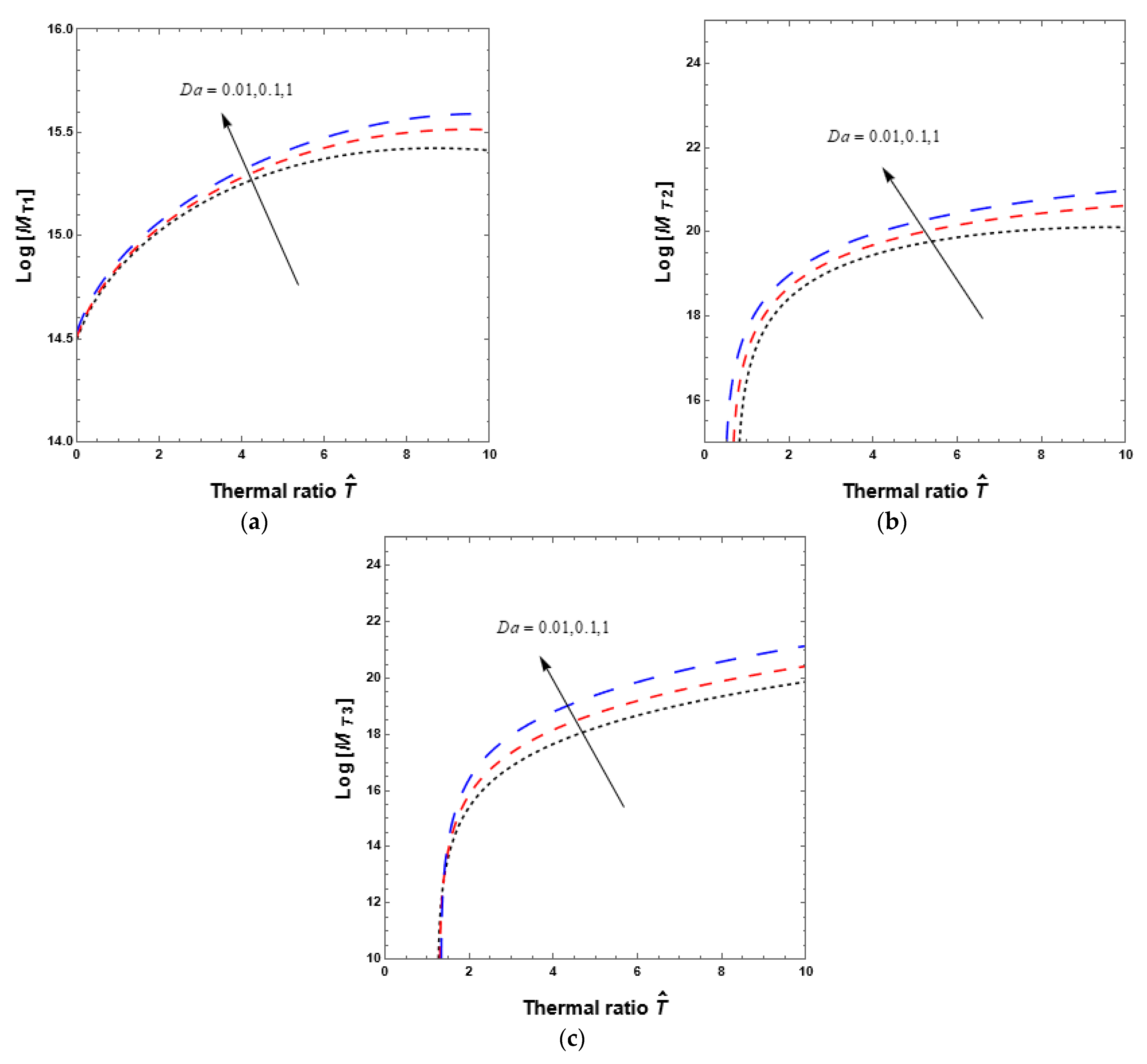
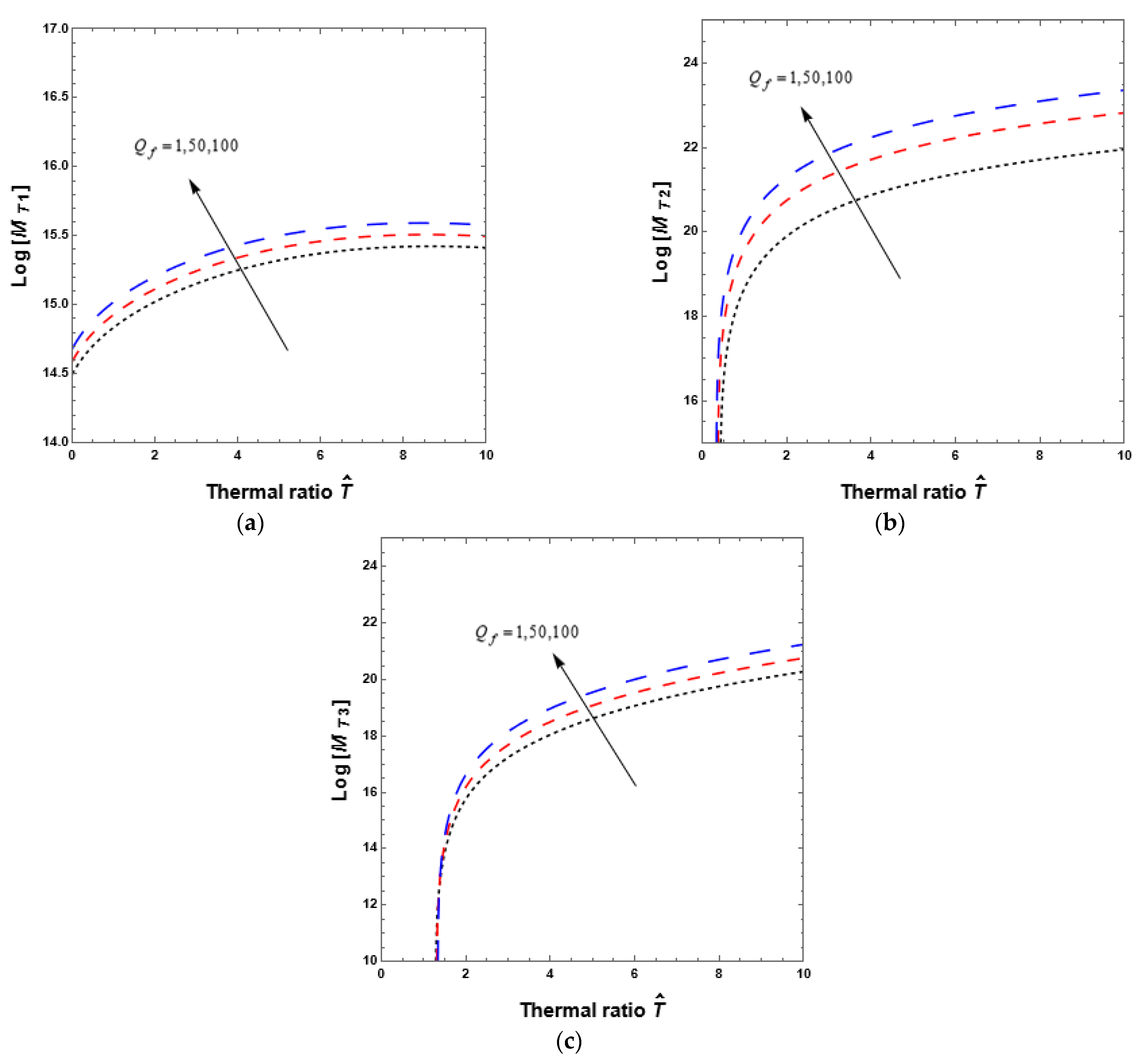
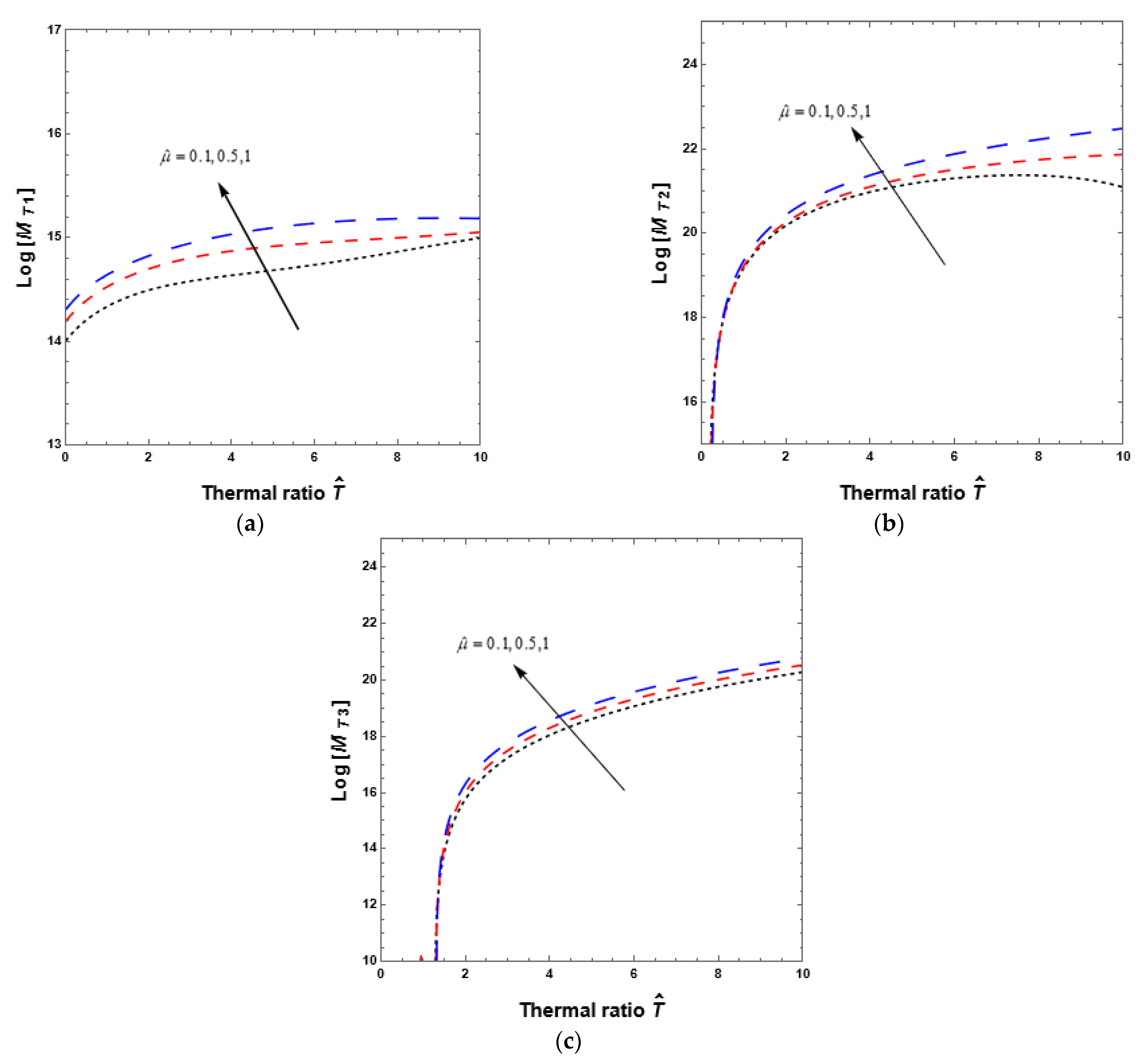
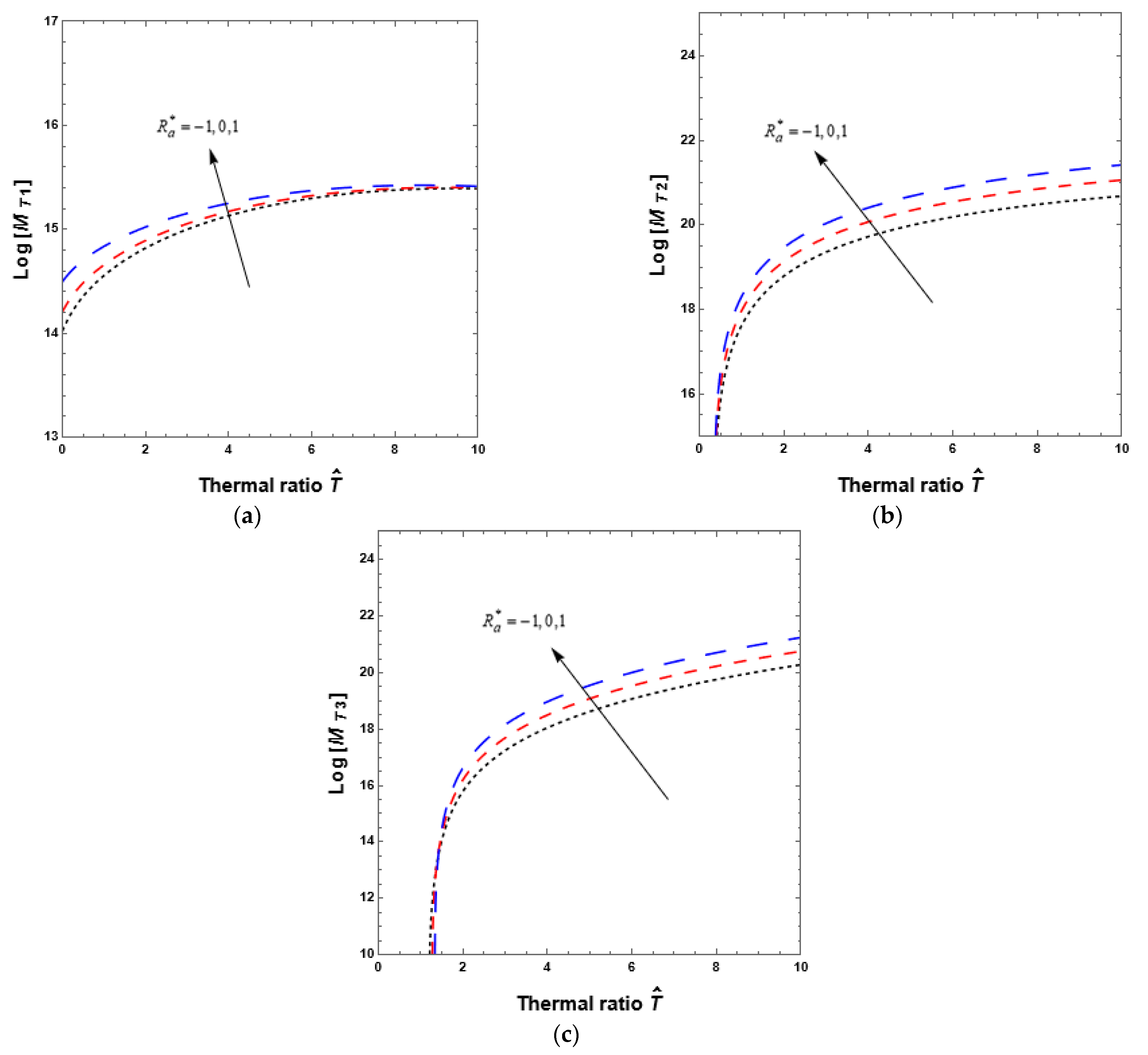
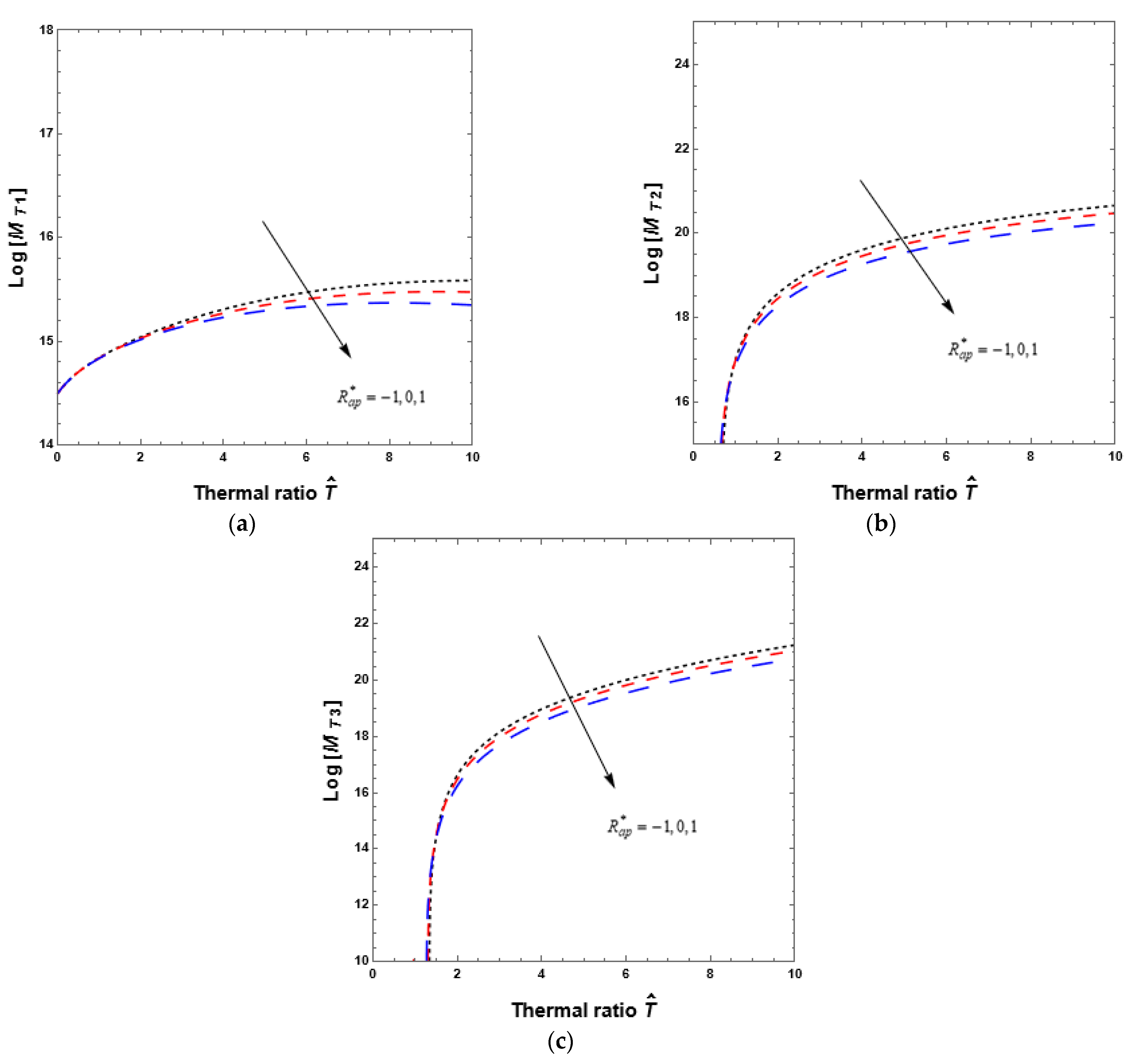
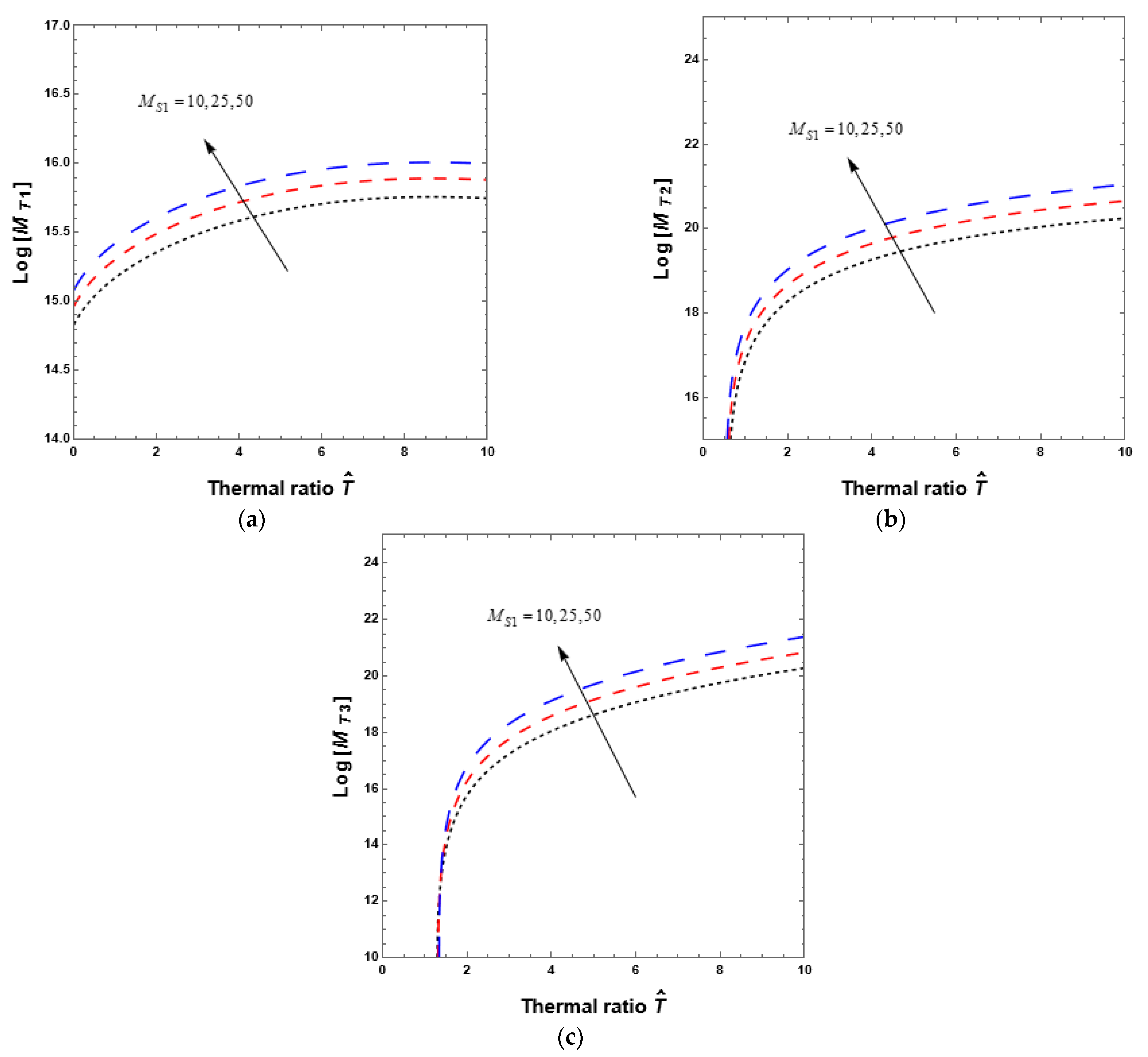
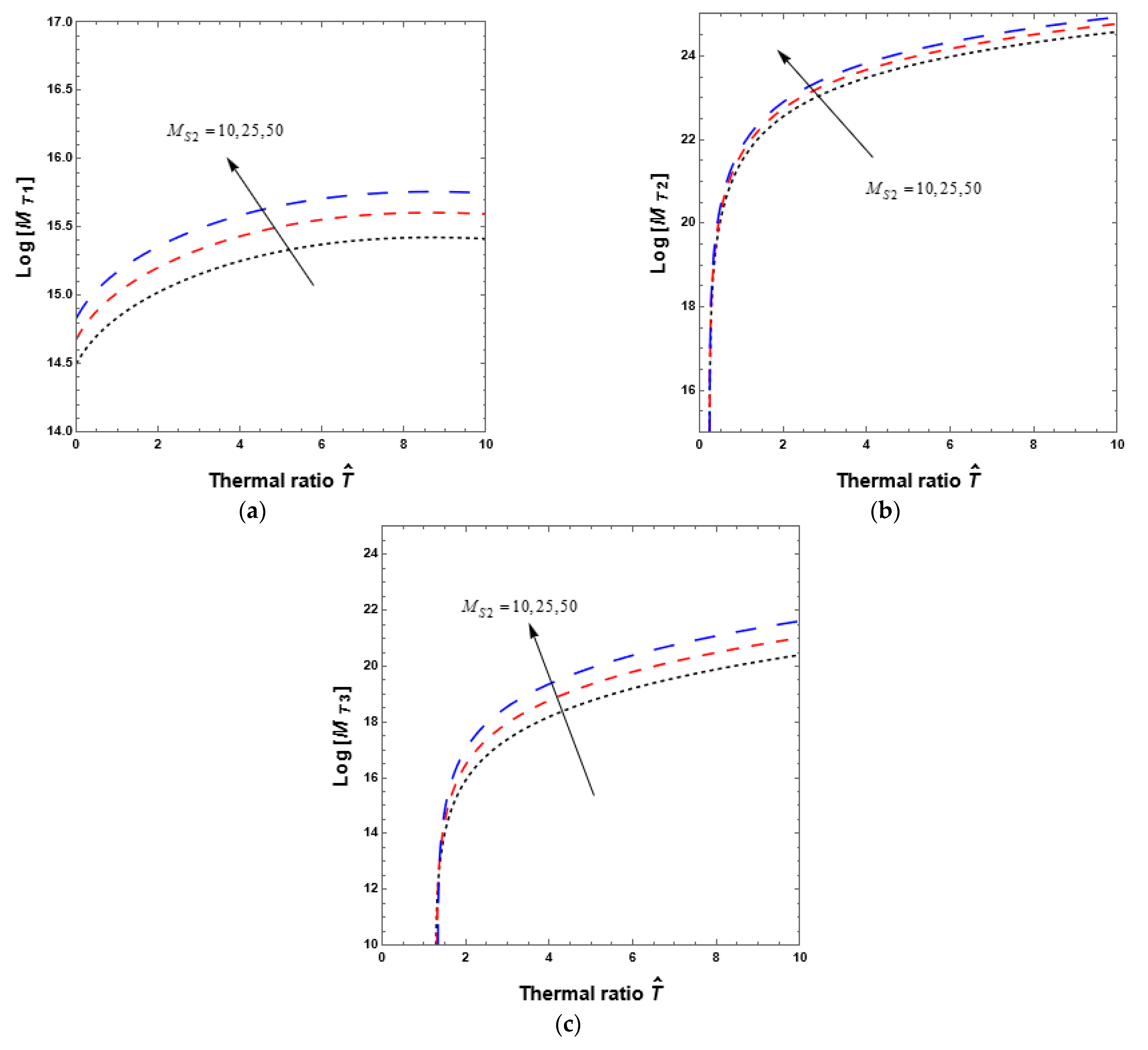
5. Results and Discussion

The three thermal Marangoni numbers (TMNs)—for the linear TP $M_{T1}$, for the parabolic TP $M_{T2}$, and for the inverted parabolic TP $M_{T3}$—are solved for BBTDMM convection in the occurrence of constant heat sources/sinks in a closed-form and uniform vertical magnetic field. These three TMNs $M_T$ are drawn against the thermal ratio $\widehat{T}$ with the logarithm of TMNs along the y-axis. The effects of permeability (in terms of Darcy number), effective viscosity ratio (in terms of viscosity ratio), heat source/sink (in terms of modified internal Rayleigh numbers), and second and third diffusing components (in terms of solute Marangoni numbers) on the three TMNs are shown in the following figures, which correspond to all three TPs.

Figure 2a for linear profile, Figure 2b for parabolic profile, and Figure 2c for inverted parabolic profile shows the effect of permeability on TMNs for all three TPs, expressed as a Darcy number for $Da=0.01,0.1,1$. With the increase in thermal ratio, the TMNs increase by a certain value, demonstrating that the system is stable, even though the fluid has a larger window. This could be due to a combination of salinity and magnetic field effects. As a result, increasing permeability delays BBTDMM convection for all TPs; this was not predicted. The Darcy number is also effective for bigger values of thermal ratios, as evidenced by the diverging curves. The effect of the magnetic field on the TMNs is shown in Figure 3a for linear, Figure 3b for parabolic, and Figure 3c for inverted parabolic profiles, for all three TPs in terms of the Chandrasekhar number $Q_f$. The TMNs rise as the value of this parameter grows; therefore, by increasing the values of this parameter, BBTDMM convection can be postponed, which is materially sensible, and bigger effective viscosity values generate flow resistance, making the system stable. The effect of the viscosity ratio $\widehat{\mu }$ on the TMNs can be seen in Figure 4a for linear profile, Figure 4b for parabolic profile, and Figure 4c for inverted parabolic profile. The TMNs rise as the value of this parameter grows; by increasing the values of this parameter, BBTDMM convection can be postponed, which is materially sensible, and larger effective viscosity values produce flow resistance, resulting in a stable system. As demonstrated in Figure 3a for linear, Figure 3b for parabolic, and Figure 3c for inverted parabolic profiles, and Figure 4a for linear profile, Figure 4b for parabolic profile, and Figure 4c for inverted parabolic profile, these parameters are also effective for greater values of the thermal ratios for parabolic and inverted parabolic TPs.

For all the three TPs, the influence of the modified internal Rayleigh number $R_a^{*}$ on the TMNs is shown in Figure 5a for linear profile, Figure 5b for parabolic profile, and Figure 5c for inverted parabolic profile. The TMNs increase as the value of this parameter grows, demonstrating that raising the value of heat from sink to source can delay BBTDMM convection. As a result of the heat absorption, the system becomes stable, which is extremely impractical. This could be due to the presence of second and third diffusing components. For the parabolic and inverted parabolic TPs, these parameters have a bigger influence at higher thermal ratios, but the linear TP shows the opposite effect. The effect of the modified internal Rayleigh number $R_{ap}^{*}$ for region II of the TMN is seen in Figure 6a for linear profile, Figure 6b for parabolic profile, and Figure 6c for inverted parabolic profile for all three TPs. As the value of this parameter increases from sink to source, the TMN decreases, allowing BBTDMM convection to be pre-scheduled by lowering the values of this parameter, which is materially perceptible, and the heat absorption in the porous layer stabilizes the system. As demonstrated in the figure, this parameter is likewise effective for a moderate value of the thermal ratios for all three TPs.

The impact of solute1 and solute2 Marangoni numbers $M_{S1}$ and $M_{S2}$ on the TMNs is compared for all the three TPs in Figure 7a for linear profile, Figure 7b for parabolic profile, and Figure 7c for inverted parabolic profile and Figure 8a for linear profile, Figure 8b for parabolic profile, and Figure 8c for inverted parabolic profile, respectively, for $M_{S1}=10,25,50$ and $M_{S2}=10,25,50$. The TMNs increase as the values of these parameters increase, and hence elevating the values of these solute Marangoni numbers for all TPs can delay BBTDMM convection in the double layer. In other words, in the presence of all TPs, the existence of second and third diffusing components delays BBTDMM convection in two layers. These factors have a significant impact when the thermal ratio is higher, as seen by the diverging curves for all parabolic and inverted parabolic TPs.

6. Conclusions

By taking into account the heat source using the Darcy–Brinkman model, the triple-diffusive magneto-convection problem with diffusing component heat and solute has been examined for three temperature profiles using an exact technique. Version 12.0 of the MATHEMATICA software was used to perform numerical calculations. The investigation’s findings are as follows, based on the results:

➢

The inverted parabolic TP on BBTDMM convection in a double layer is the most stable of all the three TPs, the linear TP is the most unstable one, and the parabolic TP is the moderate one.

➢

The study’s pertinent physical parameters hold true for higher values of thermal ratios.

➢

One can delay BBTDMM convection in two layers by raising the values of the modified internal Rayleigh number for the fluid layer and the solute Marangoni numbers, Darcy number, and viscosity ratio for the group of physical factors used in the study.

➢

An applied magnetic field stabilizes the system by postponing BBTDMM convection.

➢

The modified internal Rayleigh number for the porous region destabilizes the system. Higher values of the modified internal Rayleigh number for region II augment BBTDMM convection.

➢

The destabilizing effects under conditions of normal gravity are more effective in the production of permanent magnetic materials. It is possible to create a high-quality permanent magnetic material by increasing the modified internal Rayleigh number for the porous medium.

➢

The findings are in good agreement with earlier research articles.

References

1. Ravi, S.K.; Singh, A.K.; Alawadhi, K.A. Effect of temperature dependent heat source/sink on free convective flow of a micropolar fluid between two vertical walls. Int. J. Energy Technol. 2011, 3, 1–8. [Google Scholar]
2. Liu, I.-C.; Wang, H.-H.; Umavathi, J.C. Effect of viscous dissipation, internal heat source/sink, and thermal radiation on a hydromagnetic liquid film over an unsteady stretching sheet. J. Heat Transf. 2013, 135, 031701. [Google Scholar] [CrossRef]
3. Srinivasacharya, D.; Surender, O. Non-Darcy mixed convection in a doubly stratified porous medium with Soret-Dufour effects. Int. J. Eng. Math. 2014, 2014, 126218. [Google Scholar] [CrossRef] [Green Version]
4. Dessie, H.; Kishan, N. MHD effects on heat transfer over stretching sheet embedded in porous medium with variable viscosity, viscous dissipation and heat source/sink. Ain Shams Eng. J. 2014, 5, 967–977. [Google Scholar] [CrossRef] [Green Version]
5. Gireesha, B.J.; Mahanthesh, B.; Rashidi, M.M. MHD boundary layer heat and mass transfer of a chemically reacting Casson fluid over a permeable stretching surface with non-uniform heat source/sink. Int. J. Ind. Math. 2015, 7, 247–260. [Google Scholar]
6. Hayat, T.; Awais, M.; Imtiaz, A. Heat source/sink in a magneto-hydrodynamic non-Newtonian fluid flow in a porous medium: Dual solutions. PLoS ONE 2016, 11, e0162205. [Google Scholar] [CrossRef] [Green Version]
7. Mabood, F.; Ibrahim, S.M.; Rashidi, M.M.; Shadloo, M.S.; Lorenzini, G. Non-uniform heat source/sink and Soret effects on MHD non-Darcian convective flow past a stretching sheet in a micropolar fluid with radiation. Int. J. Heat Mass Transf. 2016, 93, 674–682. [Google Scholar] [CrossRef]
8. Oni, M.O. Combined effect of heat source, porosity and thermal radiation on mixed convection flow in a vertical annulus: An exact solution. Eng. Sci. Tech. Int. J. 2017, 20, 518–527. [Google Scholar] [CrossRef]
9. Hakeem, A.K.A.; Ganga, B.; Ansari, S.M.Y.; Ganesh, N.V.; Rahman, M.M. Nonlinear studies on the effect of non-uniform heat generation/absorption on hydromagnetic flow of nanofluid over a vertical plate. Nonlinear Anal. Model. Control 2017, 22, 1–16. [Google Scholar]
10. Venkateswara Raju, K.; Reddy, S.R.R.; Bala Anki Reddy, P. Effects of viscous dissipation and non-uniform heat source/sink on Casson fluid flow over an unsteady inclined permeable stretching surface. Int. J. Sci. Res. Math. Stat. Sci. 2018, 5, 130–136. [Google Scholar]
11. Khan, Z.; Rasheed, H.U.; Alkanhal, T.A.; Ullah, M.; Khan, I.; Tlili, I. Effect of magnetic field and heat source on Upper-convected-Maxwell fluid in a porous channel. Open Phys. 2018, 16, 917–928. [Google Scholar] [CrossRef]
12. Melathil, G.; Pranesh, S.; Tarannum, S. Effects of magnetic field and internal heat generation on triple diffusive convection in an Oldroyd-B liquid. Int. J. Res. Advent Technol. 2019, 7, 154–163. [Google Scholar] [CrossRef]
13. Archana, M.; Gireesha, B.J.; Prasannakumara, B.C. Triple diffusive flow of Casson nanofluid with buoyancy forces and nonlinear thermal radiation over a horizontal plate. Arch. Thermodyn. 2019, 40, 49–69. [Google Scholar]
14. Rana, P.; Agarwal, S.; Bhardwaj, A. Triple diffusive convection study of a binary nanofluid saturated rotating porous layer under the influence of magnetic field. Int. J. Comput. Methods Eng. Sci. Mech. 2019, 20, 395–403. [Google Scholar] [CrossRef]
15. Manjunatha, N.; Sumithra, R. Effects of non-uniform temperature gradients on triple diffusive surface tension driven magneto convection in a composite layer. Univers. J. Mech. Eng. 2019, 7, 398–410. [Google Scholar]
16. Taiwo, Y.S.; Gambo, D.; Olaife, A.H. Effect of heat source/sink on MHD start-up natural convective flow in an annulus with isothermal and isoflux boundaries. Arab J. Basic Appl. Sci. 2020, 27, 365–374. [Google Scholar] [CrossRef]
17. Jha, B.K.; Samaila, G. Impact of temperature dependent heat source on MHD natural convection flow between two vertical plates filled with nanofluid with induced magnetic field effect. Arab J. Basic Appl. Sci. 2020, 27, 299–312. [Google Scholar] [CrossRef]
18. Thumma, T.; Mishra, S.R. Effect of nonuniform heat source/sink, and viscous and Joule dissipation on 3D Eyring–Powell nanofluid flow over a stretching sheet. J. Comput. Des. Eng. 2020, 7, 412–426. [Google Scholar] [CrossRef]
19. Dwivedi, N.; Singh, A.K. Transient free convective hydromagnetic flow in an infinite vertical cylinder with Hall current and heat source/sink. Heat Transf. 2020, 49, 4091–4108. [Google Scholar] [CrossRef]
20. Singh, A.K. Role of heat source/sink in transient free convective flow through a vertical cylinder filled with a permeable medium: An analytical approach. Heat Transf. 2021, 50, 3154–3175. [Google Scholar]
21. Singh, A.K.; Chandran, P.; Sacheti, N.C. Effect of Newtonian heating/cooling on free convection in an annular permeable region in the presence of heat source/sink. Heat Transf. 2021, 50, 712–732. [Google Scholar]
22. Rudziva, M.; Sibanda, P.; Noreldin OA, I.; Goqo, S. On trigonometric cosine, square, sawtooth, and triangular wave-type rotational modulations on triple-diffusive convection in salted water. Heat Transf. 2021, 50, 6886–6914. [Google Scholar] [CrossRef]
23. Pranesh, S.; Siddheshwar, P.G.; Zhao, Y.; Mathew, A. Linear and nonlinear triple diffusive convection in the presence of sinusoidal/non-sinusoidal gravity modulation: A comparative study. Mech. Res. Commun. 2021, 113, 103694. [Google Scholar] [CrossRef]
24. Nagendramma, V.; Durgaprasad, P.; Sivakumar, N.; Rao, B.M.; Raju, C.S.K.; Shah, N.A.; Yook, S.J. Dynamics of triple diffusive free convective MHD fluid flow: Lie group transformation. Mathematics 2022, 10, 2456. [Google Scholar] [CrossRef]
25. Zainodin, S.; Jamaludin, A.; Nazar, R.; Pop, I. MHD mixed convection of hybrid ferrofluid flow over an exponentially stretching/shrinking surface with heat source/sink and velocity slip. Mathematics 2022, 10, 4400. [Google Scholar] [CrossRef]
26. Lakshmi Devi, G.; Niranjan, H. The novelty of thermo-diffusion and diffusion-thermo, slip, temperature and concentra-tion boundary conditions on magneto–chemically reactive fluid flow past a vertical plate with radiation. Symmetry 2022, 14, 1496. [Google Scholar] [CrossRef]
27. Kune, R.; Naik, H.S.; Reddy, B.S.; Chesneau, C. Role of nanoparticles and heat source/sink on MHD flow of Cu-H2O nanofluid flow past a vertical plate with Soret and Dufour effects. Math. Comput. Appl. 2022, 27, 102. [Google Scholar] [CrossRef]
28. Kaleem, M.M.; Usman, M.; Asjad, M.I.; Eldin, S.M. magnetic field, variable thermal conductivity, thermal radiation, and viscous dissipation effect on heat and momentum of fractional Oldroyd-B bio nano-fluid within a channel. Fractal Fract. 2022, 6, 712. [Google Scholar] [CrossRef]
29. Khan, U.; Zaib, A.; Ishak, A.; Alotaibi, A.M.; Eldin, S.M.; Akkurt, N.; Waini, I.; Madhukesh, J.K. Stability analysis of buoyancy magneto flow of hybrid nanofluid through a stretchable/shrinkable vertical sheet induced by a micropolar fluid subject to nonlinear heat sink/source. Magnetochemistry 2022, 8, 188. [Google Scholar] [CrossRef]
30. Khan, Y.; Akram, S.; Razia, A.; Hussain, A.; Alsulaimani, H.A. Effects of double diffusive convection and inclined magnetic field on the peristaltic flow of fourth grade nanofluids in a non-uniform channel. Nanomaterials 2022, 12, 3037. [Google Scholar] [CrossRef]
31. Rafeek, K.V.M.; Reddy, G.J.; Ragoju, R.; Reddy, G.S.K.; Sheremet, M.A. Impact of throughflow and coriolis force on the onset of double-diffusive convection with internal heat source. Coatings 2022, 12, 1096. [Google Scholar] [CrossRef]
32. Corcione, M.; Quintino, A. Double-diffusive effects on the onset of Rayleigh-Bènard convection of water-based nanofluids. Appl. Sci. 2022, 12, 8485. [Google Scholar] [CrossRef]
33. Liu, C.; Knobloch, E. Single-mode solutions for convection and double-diffusive convection in porous media. Fluids 2022, 7, 373. [Google Scholar] [CrossRef]
34. Manjunatha, N.; Sumithra, R. Effects of heat source/sink on Darcian-Bènard-Magneto-Marangoni convection in a composite layer subjected to non-uniform temperature gradients. TWMS J. Appl. Eng. Math. 2022, 12, 669–684. [Google Scholar]
35. Manjunatha, N.; Sumithra, R.; Vanishree, R.K. Influence of constant heat source/sink on non-Darcian-Bènard double diffusive Marangoni convection in a composite layer system. JAMI J. Appl. Math. Inform. 2022, 40, 99–115. [Google Scholar]
36. Barna, I.F.; Bognár, G.; Mátyás, L.; Hriczó, K. Self-similar analysis of the time-dependent compressible and incompressible boundary layers including heat conduction. J. Therm. Anal. Calorim. 2022, 147, 13625–13632. [Google Scholar] [CrossRef]
37. Barna, I.F.; Mátyás, L. Analytic self-similar solutions of the Oberbeck-Boussinesq equation. Chaos Solitons Fractals 2015, 78, 249–255. [Google Scholar] [CrossRef] [Green Version]
38. Shivakumara, I.S.; Rudraiah, N.; Nanjundappa, C.E. Effect of non-uniform basic temperature gradient on Rayleigh-Benard-Marangoni convection in ferrofluids. J. Magn. Magn. Mater. 2002, 248, 379–395. [Google Scholar] [CrossRef]
39. Shiva kumara, I.S.; Suma, S.P.; Chavaraddi, K.B. Onset of surface tension driven convection in superposed layers of fluid and saturated porous medium. Arch. Mech. 2006, 58, 71–92. [Google Scholar]
40. Shivakumara, I.S.; Sureshkumar, S.; Devaraju, N. Effect of non-uniform temperature gradients on the onset of convection in a couple-stress fluid-saturated porous medium. J. Appl. Fluid Mech. 2012, 5, 49–55. [Google Scholar] [CrossRef]
41. Sparrow, E.M.; Goldstein, R.J.; Jonson, V.K. Thermal instability in a horizontal fluid layer effect of boundary conditions and non-linear temperature profile. J. Fluid. Mech 1964, 18, 513. [Google Scholar] [CrossRef]
Figure 1. Physical model of the problem.
Symmetry 15 00644 g001
Figure 2. (a) for linear profile, (b) for parabolic profile, and (c) for inverted parabolic profile. Effects of Darcy number D a on TMN when a f = 1 , d ^ = 1 , μ ^ = 1.5 , S ^ 1 = S ^ 2 = 1 , τ f 1 = τ f 2 = 0.25   τ p 1 = τ p 2 = 0.25 , Q f = 10 , M S 1 = 10 , M S 2 = 15 , R a * = R a p * = 1 .
Symmetry 15 00644 g002
Figure 3. (a) for linear profile, (b) for parabolic profile, and (c) for inverted parabolic profile. Effects of Chandrasekhar number Q f effects in region I on TMN when a f = 1 , d ^ = 1 , D a = 1.0 , μ ^ = 1.5 , S ^ 1 = S ^ 2 = 1 , τ f 1 = τ f 2 = τ p 1 = τ p 2 = 0.25 , M S 1 = 10 , M S 2 = 15 , R a * = R a p * = 1 .
Symmetry 15 00644 g003
Figure 4. (a) for linear profile, (b) for parabolic profile, and (c) for inverted parabolic profile. Effects of viscosity ratio μ ^ effects in region II on TMN when a f = 1 , d ^ = 1 , D a = 1.0 , μ ^ = 1.5 , S ^ 1 = S ^ 2 = 1 , τ f 1 = τ f 2 = 0.25   τ p 1 = τ p 2 = 0.25 , Q f = 10 , M S 1 = 10 , M S 2 = 15 , R a * = R a p * = 1 .
Symmetry 15 00644 g004
Figure 5. (a) for linear profile, (b) for parabolic profile, and (c) for inverted parabolic profile. Modified internal Rayleigh number R a * on TMN when a f = 1 , d ^ = 1 , D a = 1.0 , μ ^ = 1.5 , S ^ 1 = S ^ 2 = 1 , τ f 1 = τ f 2 = τ p 1 = τ p 2 = 0.25 ,   Q f = 10 , M S 1 = 10 , M S 2 = 15 , R a p * = 1 .
Symmetry 15 00644 g005
Figure 6. (a) for linear profile, (b) for parabolic profile, and (c) for inverted parabolic profile. Modified internal Rayleigh number R a p * on TMN when a f = 1 , d ^ = 1 , D a = 1.0 , μ ^ = 1.5 , S ^ 1 = S ^ 2 = 1 , τ f 1 = τ f 2 = τ p 1 = τ p 2 = 0.25 ,   Q f = 10 , M S 1 = 10 , M S 2 = 15 , R a * = 1 .
Symmetry 15 00644 g006
Figure 7. (a) for linear profile, (b) for parabolic profile and (c) for inverted parabolic profile. Effects of solute1 Marangoni number M S 1 on TMN when a f = 1 , d ^ = 1 , D a = 1.0 , μ ^ = 1.5 , S ^ 1 = S ^ 2 = 1 , τ f 1 = τ f 2 = τ p 1 = τ p 2 = 0.25 , Q f = 10 , M S 2 = 15 , R a * = R a p * = 1 .
Symmetry 15 00644 g007
Figure 8. (a) for linear profile, (b) for parabolic profile and (c) for inverted parabolic profile. Effects of solute2 Marangoni number M S 2 on TMN when a f = 1 , d ^ = 1 , D a = 1.0 , μ ^ = 1.5 , S ^ 1 = S ^ 2 = 1 , τ f 1 = τ f 2 = τ p 1 = τ p 2 = 0.25 , Q f = 10 , M S 1 = 10 , R a * = R a p * = 1 .
Symmetry 15 00644 g008