Wobbling Fractals for The Double Sine–Gordon Equation

Abstract

This paper studies a perturbative approach for the double sine–Gordon equation. Following this path, we are able to obtain a system of differential equations that shows the amplitude and phase modulation of the approximate solution. In the case λ = 0, we get the well-known perturbation theory for the sine–Gordon equation. For a special value $\lambda$ = −1/8, we derive a phase-locked solution with the same frequency of the linear case. In general, we obtain both coherent (solitary waves, lumps and so on) solutions as well as fractal solutions. Using symmetry considerations, we can demonstrate the existence of envelope wobbling solitary waves, due to the critical observation the phase modulation depending on the solution amplitude and on the position. Because the double sine–Gordon equation has a very rich behavior, including wobbling chaotic and fractal solutions due to an arbitrary function in its solution, the main conclusion is that it is too reductive to focus only on coherent solutions.

1. Introduction

Nonlinear evolution equations are a fundamental topic in the scientific literature and many times we obtain approximate solution and study their behavior, even if there are nonlinear integrable equations of applicative relevance with analytical solutions and solitons [1].

The double sine–Gordon (DSG) equation was studied in many physical problems. It describes spin waves in superfluid ³He, self-induced transparency in accounting degeneracy of atomic levels [2], electromagnetic waves propagation in semiconductor quantum superlattices [3], etc.

Numerical studied have been devoted to the double sine–Gordon equation, mainly about the kink–anti-kink interaction. Moreover, starting from the numerical scheme, with a theoretical analysis, we can derive the stability and convergence results [4]

A completely different topic is studied in [5]: the chaotic motion of the driven and damped double sine–Gordon equation. Homoclinic and heteroclinic chaos are detected by the Melnikov method. The corresponding Melnikov functions are derived. A numerical method to estimate the Melnikov integral is given, and its effectiveness is illustrated through an example. Numerical simulations of homoclinic and heteroclinic chaos are precisely demonstrated through several examples. Further, a state feedback control method has been performed to suppress both homoclinic and heteroclinic chaos simultaneously. At last, numerical simulations are utilized to prove the validity of control methods [5].

We underline that at least two physical problems are described by the DSG equation, the propagation of ultra-short optical pulses in a resonant five-fold degenerate medium and the creation and propagation of spin waves in the anisotropic magnetic liquids ³HeA and ³HeB at temperatures below the transition to the A phase at 2.6 mK [6].

The optical pulse problem is governed by a double sine–Gordon equation, the ³HeA problem by the sine–Gordon and the ³HeB by a double sine–Gordon with changed sign. The double sine–Gordon equation is not integrable. In the optical case, a “wobbling” 4 pulse is seen, and experiments confirm this observation [6].

In the last years, a few papers were devoted to numerical studies for particular nonlinear equations, above all the so-called good Boussinesq equation. A Fourier pseudo-spectral method has been found for the “good” Boussinesq equation with second-order temporal accuracy [7].

In a recent paper, the exact traveling wave and numerical solutions of the good Boussinesq (GB) equation were found by employing He’s semi-inverse process and moving mesh approaches. The exact results can be shown in the form of hyperbolic trigonometric functions. The GB equation has been discretized using the finite-difference method. The accuracy and stability of the used numerical scheme have been carefully investigated. Numerical comparisons with exact traveling wave solutions can be found theoretically and graphically. We can conclude that the novel methods improve solution stability and accuracy. In conclusion, these new techniques are reliable and effective in extracting some new solutions for some nonlinear partial differential equations (NLPDEs) [5].

Moreover, a Fourier pseudo spectral method with second-order temporal accuracy can be successfully achieved [5].

The double sine–Gordon theory has been considered because it is a prototype of non-integrable field theory. We can find interesting results by application of techniques developed in the context of integrable field theories [8]. We can remind the study of massive Schwinger model (two-dimensional quantum electrodynamics) and a generalized Ashkin-Teller model (a quantum spin system) [9]. Another application to the one-dimensional Hubbard model is examined in [10]. The unperturbed DSG equation can be written as

$$\frac{{\partial }^2\varphi }{\partial t^2}-\frac{{\partial }^2\varphi }{\partial x^2}+sin\varphi +\lambda sin2\varphi =0$$

(1)

where $\varphi =\varphi \left(x,t\right)$ is the real nonlinear field under investigation. We obtain the sine–Gordon (SG) equation when λ = 0. The sine–Gordon equation was studied by Eleuch and Rostostev (see [10] and references therein).

The group derived solutions using new analytical methods, and a number of pertinent solutions were found. It is well known that the interactions of solitary waves for the DSG equation are not elastic [11,12,13], they are accompanied by radiation loss. The DSG equation can be solved using the Asymptotic Perturbation (AP) method, which has also been used in a number of resonances for the Hirota–Maccari equation [14], the Maccari system [15] and the nonlinear Schrodinger equation (parametric resonance) [16].

In Section 2, we are able to obtain an approximate solution for the DSG equation, using an independent Lorentz-invariant variable change with a slow time and a large space scale, using $\epsilon$ as a bookkeeping device, followed by a Fourier expansion.

In Section 3, we consider the coherent solutions, envelope solitary waves, phase-locked solutions, envelope lumps solutions and so on and observe the wobbling behavior of the nonlinear solution,

In Section 4, we consider stochastic fractal solutions starting from the Weierstrass function and other stochastic functions.

Conclusion and directions for future work is reserved to Section 5.

2. Building the Approximate Solution

We apply the asymptotic perturbation (AP) method to the DSG Equation (1).

First of all, we consider the following approximate equation in order to build an approximate solution for the Equation (1) and use a Taylor expansion for the nonlinear field,

$$\varphi \to \epsilon \varphi ,sin\varphi \approx \epsilon \varphi -{\epsilon }^3\frac{{\varphi }^3}{6}+h.o.t., sin2\varphi \approx 2\epsilon \varphi -4{\epsilon }^3\frac{{\varphi }^3}{3}+h.o.t.$$

(2)

$$\frac{{\partial }^2\varphi }{\partial t^2}-\frac{{\partial }^2\varphi }{\partial x^2}+\left(2\lambda +1\right)\varphi -{\epsilon }^2\left(\frac{4}{3}\lambda +\frac{1}{6}\right){\varphi }^3=0$$

(3)

where h.o.t. stands for higher order terms and $\epsilon$ is a bookkeeping device, which we will set to unity in the final analysis. The AP method is different from the multiple scales method, because it uses only two temporal scales: the fast (t) and the slow ($\tau$) time. the fast scale is used to delete the higher harmonics terms; on the contrary, the slow scale describes the nonlinear effects produced by the nonlinearity.

Considering only the linear part of Equation (3), where the nonlinear term in ${\varphi }^3$ can be neglected, we find that plane waves in the form:

$$Aexp\left(iKx-\omega t\right)$$

(4)

are solutions if the following linear dispersion law is verified:

$${\omega }^2=K^2+2\lambda +1$$

(5)

where A is a constant term, K the wave number and $\omega$ the circular frequency. The dispersion law allows us to understand how the wave number K, i.e., the wavelength

$$\lambda =\frac{2\pi }{K}$$

(6)

modifies the circular frequency $\omega$.

From Equation (5) we can obtain the relative group velocity:

$$V_G=\frac{d\omega }{dK}=\frac{K}{\omega }=\frac{K}{\sqrt{K^2+2\lambda +1}}$$

(7)

Note that for large K values the group velocity becomes 1, that is the light speed. We introduce coarse grained independent variables, slow time and large space through a Lorentz-invariant transformation (speed of light c = 1)

$$\xi =\epsilon \gamma \left(x-\beta t\right)\hspace{1em}\hspace{1em}𝜏=\epsilon \gamma \left(t-\beta x\right)$$

(8)

where

$$\gamma =1/\sqrt{\left(1-{\beta }^2\right)}$$

(9)

is the usual Lorentz factor.

We use a Fourier expansion:

$$\begin{gathered} U\left(x,t\right)=\epsilon \psi \left(\epsilon ,\xi ,\tau \right)exp\left(i\left(kx-\omega t\right)\right)+{\epsilon }^3{\psi }_3\left(\epsilon ,\xi ,\tau \right)exp\left(3i\left(kx-\omega t\right)\right) \\ +\epsilon \tilde{\psi }\left(\epsilon ,\xi ,\tau \right)exp\left(-i\left(kx-\omega t\right)\right)+{\epsilon }^3\widetilde{{\psi }_3}\left(\epsilon ,\xi ,\tau \right)exp\left(-3i\left(kx-\omega t\right)\right) \\ +\dots {\epsilon }^n{\psi }_n\left(\epsilon ,\xi ,\tau \right)exp\left(-\left(Kx-\omega t\right)\right)+{\epsilon }^n\widetilde{{\psi }_n}\left(\epsilon ,\xi ,\tau \right)exp\left(-\left(Kx-\omega t\right)\right)+\dots h.o.t. \end{gathered}$$

(10)

where the wide tilde stands for complex conjugate, n is a positive odd integer and h.o.t. stands for higher order terms.

Proposition 1.

We assume that in the Fourier expansion (10) the following limit exists and is finite

$$\underset{\epsilon \to 0}{\mathit{lim}} {\psi }_n\left(\epsilon ,\xi ,\tau \right)={\psi }_n\left(\xi ,\tau \right)$$

(11)

Theorem 1.

The variable change (8–9) and the Fourier expansion (10) imply that:

$${\partial }_x\to \gamma {\partial }_{\xi }-\beta \gamma {\partial }_{\tau }+\mathit{ink}$$

(12)

$${\partial }_t\to \gamma {\partial }_{\tau }-\beta \gamma {\partial }_{\xi }-\mathit{in}\omega$$

(13)

Proof. 

This theorem follows from the observation that:

$${\partial }_x\psi \left(\xi ,\tau \right)exp\left(\left(Kx-\omega t\right)\right)\to ink\psi \left(\xi ,\tau \right)+\left(\epsilon \gamma {\partial }_{\xi }\psi \left(\xi ,\tau \right)-\epsilon \beta \gamma {\partial }_{\tau }\psi \left(\xi ,\tau \right)\right)exp\left(\left(Kx-\omega t\right)\right)$$

(14)

$${\partial }_t\psi \left(\xi ,\tau \right)exp\left(\left(Kx-\omega t\right)\right)\to -in\omega \psi \left(\xi ,\tau \right)+\left(\epsilon \gamma {\partial }_{\tau }\psi \left(\xi ,\tau \right)-\epsilon \beta \gamma {\partial }_{\xi }\psi \left(\xi ,\tau \right)\right)exp\left(\left(KX-\omega t\right)\right)$$

(15)

We now insert the Fourier expansion (10) into the Equation (3) and consider the equations for each given Fourier mode and to the same $\epsilon$magnitude.

If we consider only the leader terms (order of magnitude = $\epsilon$), we get the dispersion law for the linear part:

$$\left(K^2+2\lambda +1\right)\varphi =0$$

(16)

at the next order ${\epsilon }^2$we obtain, for n = 1, (NL = nonlinear part):

$$-2iK\left(\gamma {\psi }_{\xi }-\beta \gamma {\psi }_{\tau }\right)-2i\omega \left(\gamma {\psi }_{\tau }-\beta \gamma {\psi }_{\xi }\right)+NL=0$$

(17)

and if we choose

$$\beta =\frac{K}{\omega }=V_G$$

(18)

we can eliminate the two terms with the $\xi$ derivative.

At last, if we consider even the nonlinear terms, the Equation (3) yields:

$$+2i\gamma \left(K\beta -\omega \right){\psi }_{\tau }-N{\left|\psi \right|}^2\psi =0$$

(19)

where

$$N=\frac{4}{3}\lambda +\frac{1}{6}$$

(20)

Now we use the polar substitution:

$$\psi \left(\xi ,\tau \right)=\rho \left(\xi ,\tau \right)exp\left(i\theta \left(\xi ,\tau \right)\right)$$

(21)

and the reader can verify that the linearized equation obtained from Equation (3) can be easily solved with (21), because the linearized equation is easily solved with the dispersion law 5).

Using (21), we can derive two independent equations from (19)) and obtain:

$${\rho }_{\tau }=0$$

(22)

$$2\gamma \left(K\beta -\omega \right){\theta }_{\tau }-N{\rho }^2=0$$

(23)

and then

$$\rho =\rho \left(\xi \right)$$

(24)

arbitrary function of the independent variable, but time-constant and:

$${\theta }_{\tau }=\frac{\left(8\lambda +1\right)}{12\gamma \left(1+2\lambda \right)}{\rho }^2\left(\xi \right)=\Omega \left(\xi \right)$$

(25)

Note that we consider that the limit

$$\rho \left(\epsilon \to 0,\xi \right)=\rho \left(\xi \right)\ne 0$$

(26)

exists and is finite, then there is no need to assume that this limit becomes zero. □

Theorem 2.

There is a phase-locked solution for $\lambda =-\left(\frac{1}{8}\right)$ when the solution frequency is equal to the linear case.

Proof. 

Just look at the Equation (25). A new, exciting research field in physics is the phase-locked solution in nonlinear partial differential equations. We give here just two recent examples.

First, the fifth generation (5G) of mobile communications produces millimeter (mm) waves and an increasing number of connected devices. Second, optically assisted RF carrier generation are necessary to tackle this issue, with a wide use of analog radio-over-fiber (ARoF) architectures. The most important drawback of these optical well-known methods is related to the finite coherence of lasers sources, because it can dramatically degrade data transmission in analog formats. Efficient phase noise compensation algorithms can be obtained through the use of orthogonal frequency-division multiplexing (OFDM) as the 5G standard. Experimental observations support the use of a mm-wave generation technique based on an optical phase-locked loop (OPLL) that fulfills the frequency specifications for 5G [17]. In conclusion, we can state that OPLLs is a viable solution to generate mm-wave carriers for 5G and beyond. □

Now we consider another important topic connected to phase-locked solutions.

Researchers have found that there are coherent and incoherent types of random lasers, with broadband and randomly distributed narrow-band lasing spectrum, respectively. WE underline that no fixed phase relationship has ever been observed among the lasing modes in such lasers. A new form of random lasers can be found in patterned organic–inorganic hybrid perovskite MAPbBr_3. Multiple simultaneously lasing modes are stably locked in phase so that lasing lines are achieved with equal spectral separations. In the paper [18] we find the first observation of phase locking between random lasers. It can be performed by the cascaded molecular absorption-emission or cascaded excitation-injection processes among random laser modes.

Theorem 3.

Wobbling nonlinear solutions can be observed because of the phase $\Omega \left(\xi \right)$ depending on the solution amplitude and its position.

Proof. 

Theorem 3 is the most important result of this paper, i.e., an asymptotic perturbation method is able to find a wobbling behavior in the nonlinear solutions of Equation (2). Suitable choices for the arbitrary function $\rho \left(\xi \right)$, based on the Weierstrass function and symmetry reflections, can lead to wobbling solitons. □

If we look at the Equation (25), we can find that the solutions phase depends on the amplitude $\rho$ and on the $\xi$-variable, so that fractal solutions are connected to the spatial environment.

Wobbling solutions are well known. For example, in recent papers [19,20], the scattering between a wobbling kink and a wobbling anti-kink in the standard ϕ⁴ model is numerically investigated. A careful study performs the dependence of the final velocities, wobbling amplitudes and frequencies of the scattered kinks on the collision velocity and on the initial wobbling amplitude. The fractal structure becomes more intricate due to the emergence of new resonance windows and the splitting of those arising in the non-excited kink scattering.

We can observe two dominant frequencies in the second component radiation:

(i) The first is one is three times the frequency of the orthogonal wobbling mode;

(ii) The second is the sum of the frequencies of the longitudinal and orthogonal vibration modes [19,20].

In another interesting paper, it was shown that a spectral wall, i.e., an obstacle in the dynamics of a bosonic soliton, which arises due to the transition of a normal mode into the continuum spectrum, exists after coupling the original bosonic model to fermions. This spectral wall can be found if the boson or fermion field is in an excited state. The role of internal modes in multi-kink collisions has been widely studied. Now, there is a reasonably good understanding of the impact of normal and quasi-normal modes on soliton dynamics, especially in the case of bosonic field theories in (1 + 1) dimensions. First of all, such modes may trigger, via the resonant energy transfer mechanism, a chaotic (or even fractal) structure in the final state formation in multi-kink collisions. The most prominent example of such behavior is the kink–antikink scattering in φ 4 theory, Furthermore, while passing through a spectral wall, an incoming kink–fermion bound state can be separated into purely bosonic kink, which continues to move to spatial infinity and a fermionic cloud that spreads in the region before the wall [21].

3. Coherent Solutions

There are many coherent solutions for the nonlinear Equation (3).

A solitary wave is possible with the choice

$$\gamma =1.3,\beta =0.8\hspace{1em}\hspace{1em}\rho \left(\xi \right)=\frac{A}{cosh\left(B\xi \right)}\hspace{1em}\hspace{1em}A=0.1, B=2\hspace{1em}\hspace{1em}\lambda =1$$

(27)

in such a way to obtain an envelope solitary wave given by the Equation (25).

$$U\left(x,t\right)=\frac{0.1}{cosh\left(\left(2\left(\gamma \left(x-\beta t\right)\right)\right)\right)}cos\left(0.8\left(\gamma \left(x-\beta t\right)-\left(3+{\Omega }^2\right)\right)\gamma \left(t-\beta x\right)\right)$$

(28)

where $\Omega$ is given by (25). (see Figure 1a,b)

By the phase velocity V_F = 1 that is the light speed, it is obvious that this behavior is connected to the Lorentz-invariant feature of the double sine–Gordon equation.

Theorem 4.

The nonlinear solution phase depends on the solution position, a very important feature for the double sine–Gordon equation. See Figure 2.

Proof. 

The above statement follows easily from the Equation (23).

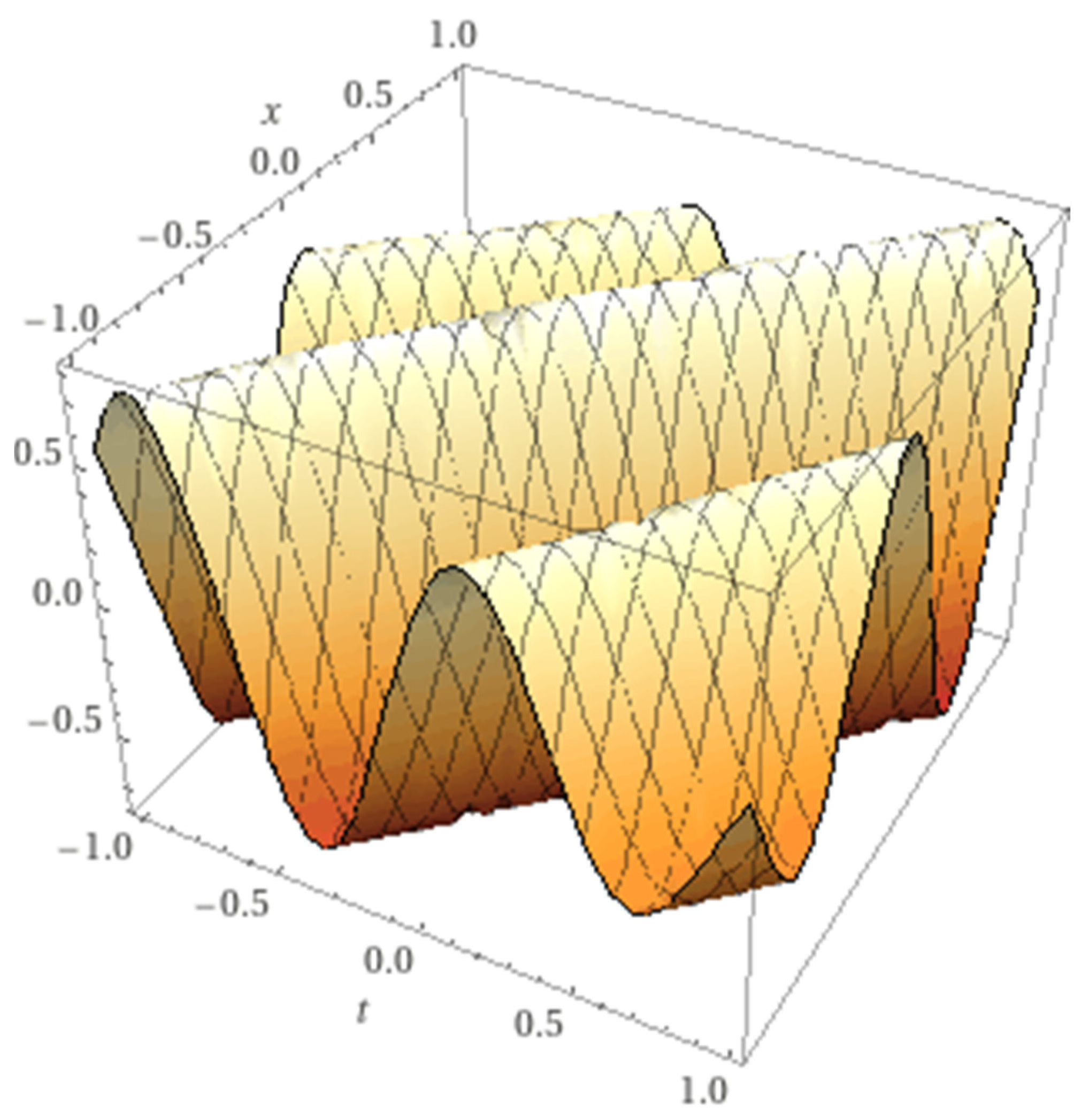
Now we study the lump phase-locked solution ($\lambda =-\left(\frac{1}{8}\right)$), see Figure 2,with the choice

$$\rho \left(\xi \right)=\frac{A}{B+C{\xi }^2}$$

(29)

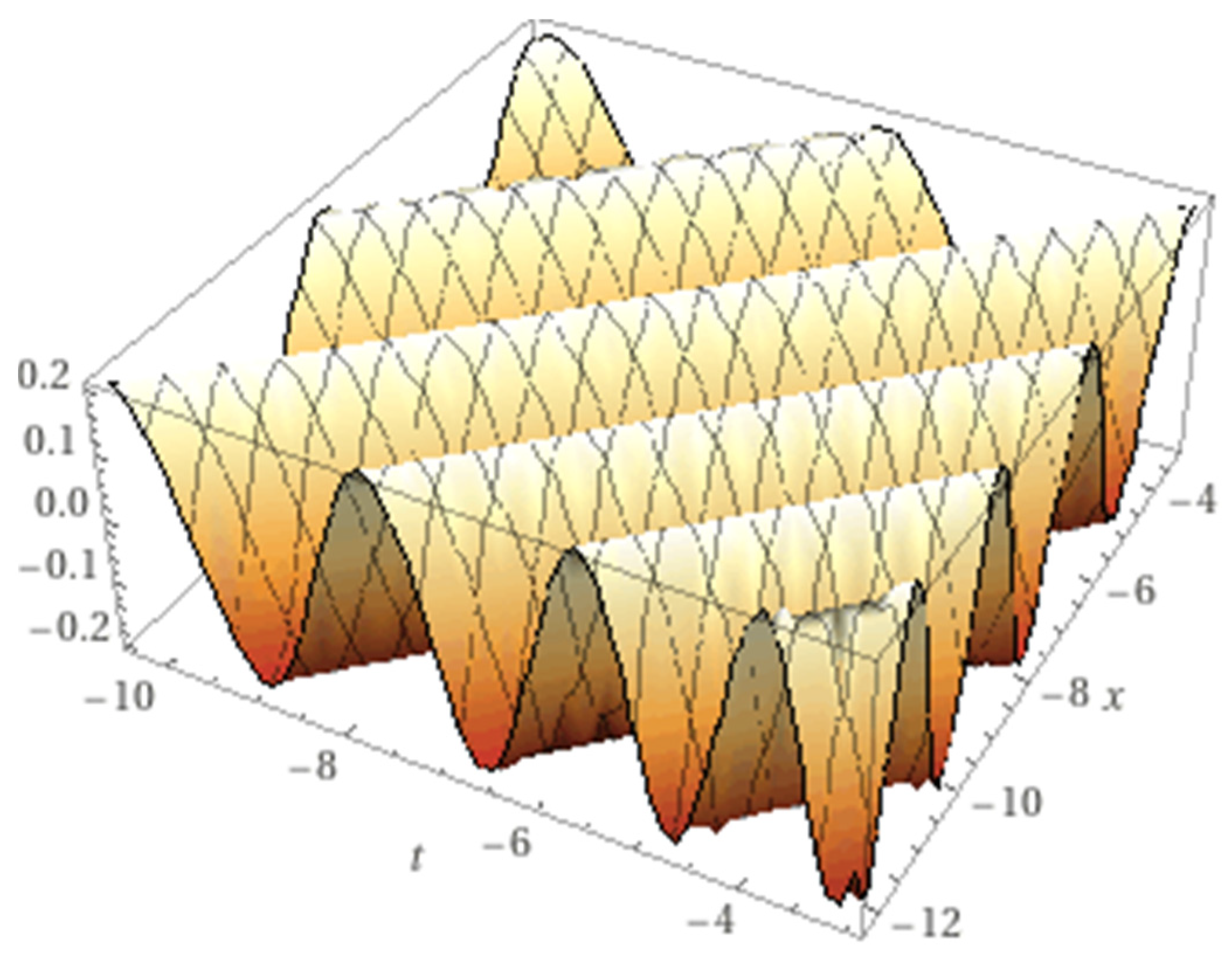
Another coherent solution is possible with the choice

$$\rho \left(\xi \right)=A{e}^{\left(B\left|\left(\xi \right)\right|\right)}$$

(30)

and it is shown in Figure 3.

See above the discussion about Theorem 4. Moreover, we can consider the chaotic and phase-locked breather dynamics in the damped and parametrically driven sine–Gordon equation [22].

4. Fractal Solutions

In this Section we show that even fractal solutions are possible for the nonlinear Equation (3). The most important feature is the arbitrary function (24) that allow us to obtain chaotic and/or fractal solutions.

We can consider the stochastic, fractal Weierstrass function W(x). This function is continuous but nowhere differentiable

$$W\left(x\right)={\displaystyle \sum }_{k=1}^N{\left(c_1\right)}^k\sin \left[{\left(c_2\right)}^{k}x\right],N\to \infty ,$$

(31)

with c₂ odd and

$$c_1{c}_2>1+\frac{3\pi }{2}$$

(32)

It is well known that the Weierstrass function (1872) was considered at the beginning a pathological function, but Weierstrass faced the most important challenge, disproving the notion that every continuous function is differentiable except on a set of isolated points. Weierstrass demonstrated that continuity did not imply almost-everywhere differentiability. It was a great breakthrough for mathematics, overturning several proofs that relied on geometric intuition and vague definitions of smoothness.

Other famous mathematicians rejected this type of functions and Henri Poincarè called it a “monster” and Weierstrass function was considered “an outrage against common sense”. Charles Hermite wrote that this function was a “lamentable scourge”. Obviously, the function was impossible to visualize until the arrival of computers in the next century, and the results did not gain wide acceptance until practical applications such as models of Brownian motion necessitated infinitely jagged functions (nowadays known as fractal curves). The Mandelbrot pioneering work changed all our beliefs about these fractal functions [23].

Fractals are everywhere. The most important concept in fractals theory is self-similarity [24,25].

Self-similarity means invariance against change in scale or size, it can be found in many physical laws and a lot of phenomena in the world. Self-similarity is one of the most important symmetries that shape our Universe. Symmetry itself is one of the most fundamental concepts in physics [24], and involves an invariance against change, for instance, “the flipping sides”. Many living bodies are built in nearly symmetric way. Even in Newton’s laws, there is no difference between right and left.

We recall, however, that the violation of the parity symmetry in weak interactions has convinced all the physicists to understand the difference between right and left. We must recall, however, that the non-conservation of parity in radioactive decay, i.e., the violation of the parity symmetry in the weak interactions was the most important topic to understand better the difference between left and right.

The fundamental work of Felix Hausdorff and Abram Besicovitch gave us a powerful tool to study self-similarity objects (the Hausdorff dimension).

Recently, a new method was proposed, the bilinear neural network method (BNNM), to find exact solutions to nonlinear partial differential equations. First, new, test functions are constructed using specific activation functions of a single-layer model, specific activation functions of “2-2” model and arbitrary functions of “2-2-3” model [26]. By means of the BNNM, nineteen sets of exact analytical solutions and twenty-four arbitrary function solutions of the dimensionally reduced p-gBKP equation are obtained via symbolic computation. The fractal solitons waves are obtained by choosing appropriate values and the self-similar characteristics of these waves are observed by reducing the observation range and amplifying the partial picture. By giving a specific activation function in the single layer neural network model, exact periodic waves and breathers are obtained. Through various three-dimensional plots, contour plots and density plots, the evolution characteristics of these waves are exhibited. [26].

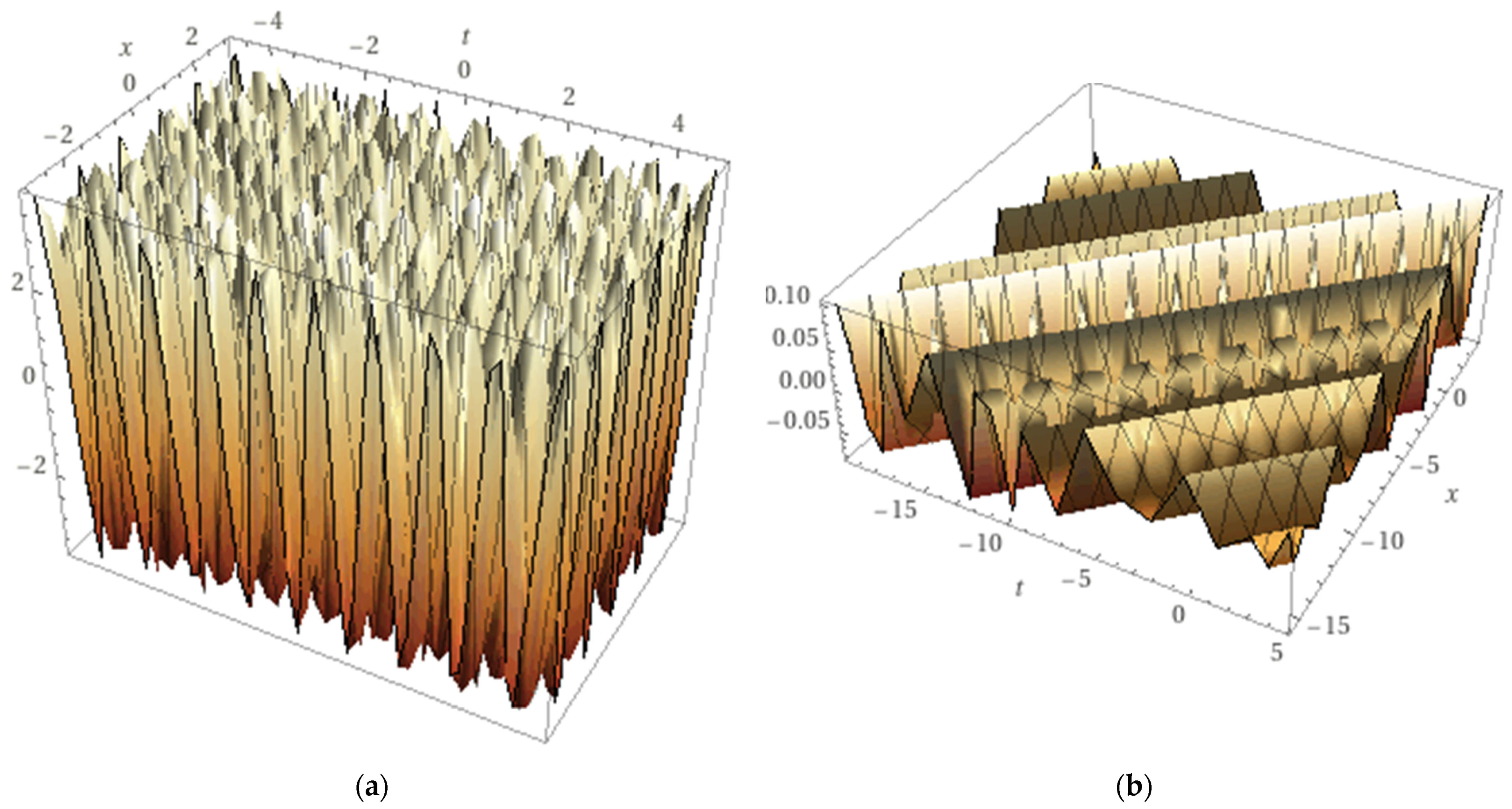
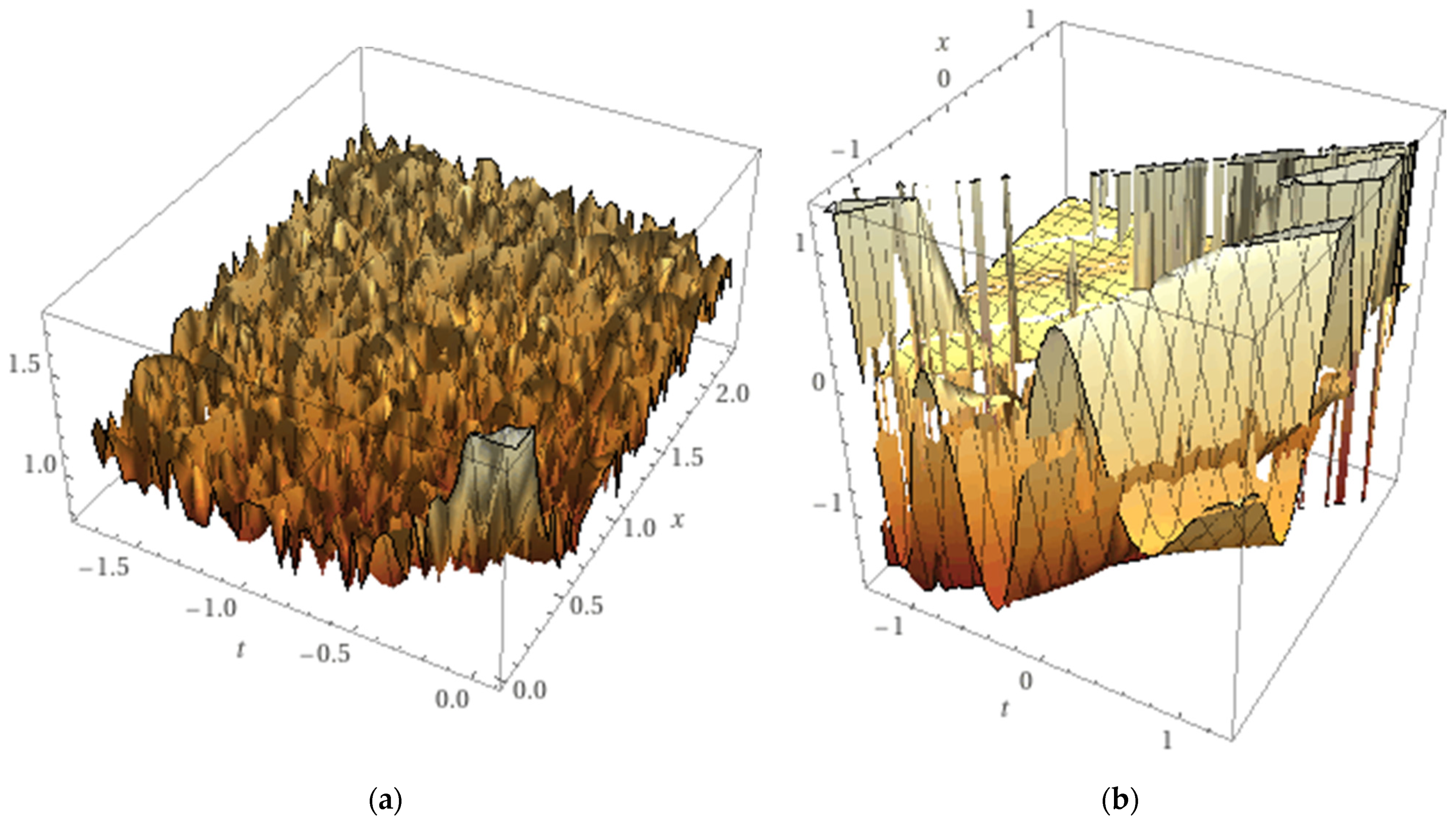
We display in Figure 4, the stochastic fractal lump solution, for simplicity we consider N = 5 and calculate the approximate Solution. We find a new type of solutions, the wobbling fractals.

$$\varphi \left(x,t\right)=W\left(\xi \right)cos\left(K\gamma \left(x-\beta t\right)-\left(\omega +\Omega \right)\gamma \left(t-\beta x\right)\right)\frac{A}{B+C{\xi }^2}$$

(33)

where $\xi$ is given by (8)) and $\Omega \left(\xi \right)$ by (25)

Note the wobbling behavior, that is, the fractal behavior, depends on the phase solution and the position. The third unlabeled axis represents the U(x,t) approximate solution function.

If we choose this fractal solution, we can see that the field U(x,t) is excited everywhere and loses all its previous coherence. These solutions have been neglected so far because they have been interpreted as noise.

Spatially coarse-grained (or effective) versions of nonlinear partial differential equations must because used together with a model for the unresolved small scales. For systems that are known to display fractal scaling, a recent paper proposed a model based on synthetically generating a scale-invariant field at small scales using fractal interpolation, and then analytically studied its effects on the large, resolved scales. The procedure was illustrated for the forced Burgers equation, that has been solved numerically on a coarse grid. Detailed comparisons with direct simulation of the full Burgers equation and with an effective viscosity model have been investigated [27].

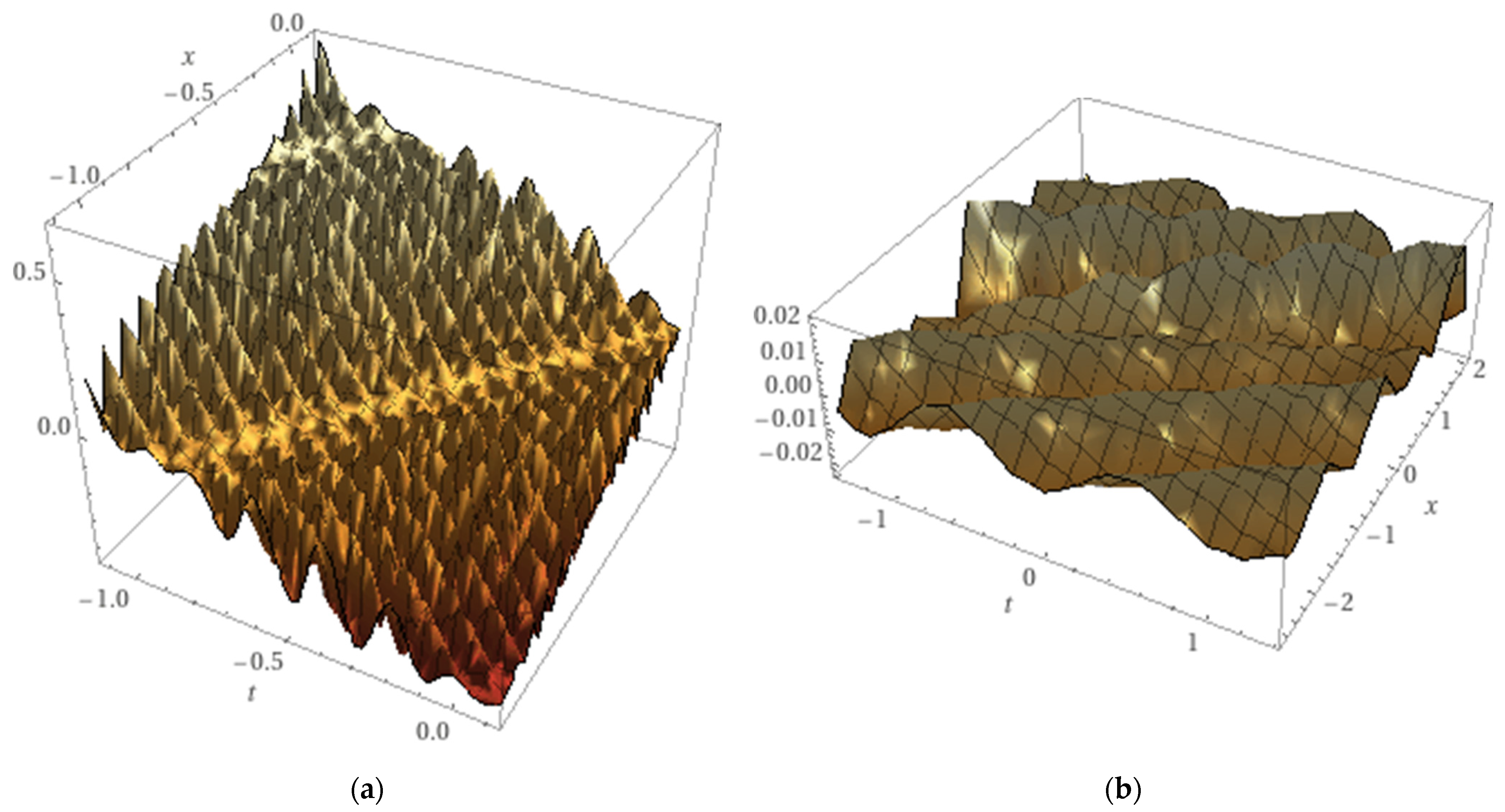
A fractal lump solution is algebraically localized in large scale and possesses self-similar structure near the center of the lump. We consider for example an amplitude fractal dromion:

$$\rho \left(\xi \right)=Rexp\left(-C\left(\left|\gamma \left(x-\beta t\right)\right|\right)\right),$$

(34)

and R is given by:

$$R=2+\sin \left(ln\left(T^2\right)\right).$$

(35)

where T is

$$T=W\left(\xi \right)=W\left(\gamma \left(x-\beta t\right)\right)$$

(36)

If we look at Figure 5a,b, we can understand that the fractal solution can arise when the initial condition is described by a fractal function and the experience and the Mandelbrot pioneering work teach us that fractals are everywhere [24].

In an interesting paper, the appearance of fractal solutions of linear and nonlinear dispersive partial differential equation on the torus was studied. Firstly, fractal solutions of linear Schrödinger equation and equations with higher-order dispersion were considered. Subsequently, applications to their nonlinear counterparts, such as the cubic Schrödinger equation and the Korteweg–de Vries equation, were carefully investigated. This paper connects with our work because both consider fractal solutions in nonlinear partial differential equations [28].

The novelty is now that we consider wobbling fractals a behavior researchers found only in some coherent solutions, such as the kink-antikink in the sine–Gordon equation.

5. Conclusions

We applied the AP method to the DSG Equation (3), considering a Lorentz-invariant change of variables with slow time and large space scale. We introduce a parameter $\lambda$ in such a way that, for $\lambda$ = 0, we obtain the standard sine–Gordon nonlinear equation.

Considering the phase modulation, we demonstrated the existence of wobbling nonlinear solutions with the phase depending on the solution amplitude and position.

Moreover, for $\lambda$ = −1/8, we obtain a phase-locked solution and show its behavior.

Nonlinear partial differential equations with phase-locked solutions can be of applicative relevance [18,19].

The AP method is then able to obtain wobbling fractal solutions, using also symmetry considerations. In the past, these fractals were considered simply as noise. Future work can be devoted to find wobbling fractal solutions for other nonintegrable nonlinear equation.

References

- Grira, S.; Boutabba, N.; Eleuch, H. Exact solutions of the Bloch equations of a two-level atom driven by the generalized double exponential quotient pulses with dephasing. Mathematics 2022, 10, 2105. [Google Scholar] [CrossRef]
- Salado, G.A.N.J.A.; Gibbs, H.E.M.; Churchill, G.C. Effects of Degeneracy on Self-Induced Transparency. Phys. Rev. Sett. 1974, 33, 273–277. [Google Scholar]
- Kr’uchkov, S.V.; Shapovalov, A.I. Effect of a high-frequency electric field on the shape of a solitary wave in a superlattice with a spectrum beyond the framework of the nearest neighbors approximation. Sov. Opt. Spectrosc. 1998, 2, 286–291. [Google Scholar]
- Campbell, D.K.; Michel, M.; Sodano, P. Kink-antikink interactions in the double sine-Gordon equation. Phys. D Nonlinear Phenom. 1986, 19, 165–205. [Google Scholar] [CrossRef]
- Xia, Z.; Yang, X. A second order accuracy in time, Fourier pseudo-spectral numerical scheme for “Good” Boussinesq equation. Discret. Contin. Dyn. Syst.-Ser. B 2022, 27, 7151–7167. [Google Scholar] [CrossRef] [Green Version]
- Bullough, R.K.; Caudrey, P.J.; Gibbs, H.M. The Double Sine-Gordon Equations: A physically applicable system of equations. In Solitons, Lectures on Current Physics; Bullough, R.K., Caudrey, P.J., Eds.; Springer: New York, NY, USA, 2011; pp. 107–141. [Google Scholar]
- Almatrafi, M.B.; Alharbi, A.R.; Tunc, C. Constructions of the soliton solutions to the Good Boussinesq equation. Adv. Differ. Equ. 2020, 29, 3089–3097. [Google Scholar] [CrossRef]
- Ablowitz, M.J.; Kruskal, M.D.; Ladik, J.F. Solitary wave collisions. SIAM J. Appl. Math. 1979, 36, 428–434. [Google Scholar] [CrossRef]
- Bullough, R.K.; Caudrey, P.J. The Double Sine Gordon Equation, Wobbling solitons? Rocky Mt. J. Math. 1978, 8, 53–60. [Google Scholar] [CrossRef]
- Olsen, O.H.; Samuelsen, M.R. Solitary wave interaction. Wave Motion 1982, 4, 29–35. [Google Scholar] [CrossRef]
- Eleuch, H.; Rostovtsev, Y.V. Analytical solution to sine-Gordon equation. J. Math. Phys. 2010, 51, 093515. [Google Scholar] [CrossRef]
- Mason, A.L. Nonlinear Equations in Physics and Mathematics; Barut, A.O., Ed.; Reidel Publishing Company: Dordrecht, Holland, 1978; pp. 205–218. [Google Scholar]
- Mussardo, G.; Riva, V.; Sotkov, G. Semiclassical particle spectrum of double sine-Gordon model. Nucl. Phys. B 2004, 687, 189–219. [Google Scholar] [CrossRef] [Green Version]
- Goldstone, J.; Jackiw, R. Quantization of nonlinear waves. Phys. Rev. D 1975, 11, 1486. [Google Scholar] [CrossRef]
- Maccari, A. Rogue Waves Generator and Chaotic and Fractal Behavior for the Maccari System with a Resonant Parametric Excitation. Symmetry 2022, 14, 2321–2329. [Google Scholar] [CrossRef]
- Maccari, A. Parametric Resonance for the Hirota-Maccari Equation. Symmetry 2022, 14, 1444–1451. [Google Scholar] [CrossRef]
- Maccari, A. A Reverse infinite period bifurcation for the nonlinear Schrodinger equation in 2+1 dimensions with a parametric excitation. J. Found. Appl. Phys. 2021, 8, 69–76. [Google Scholar]
- Dodane, D.; Santacruz, J.P.; Bourderionnet, J.; Rommel, S.; Feugnet, G.; Jurado-Navas, A.; Vivien, L.; Monroy, I.T. Optical phase-locked loop phase noise in 5G mm-wave OFDM ARoF systems. Opt. Commun. 2023, 526, 128872–128876. [Google Scholar] [CrossRef]
- Zhang, X.; Fu, J.H.Y.; Guo, J.; Zhang, Y.; Song, X. Phase-Locking of Random Lasers by Cascaded Ultrafast Molecular Excitation Dynamics. Laser Photonics Rev. 2023, 2200333. [Google Scholar] [CrossRef]
- Izquierdo, A.A.; Queiroga-Nunes, J.; Nieto, L.M. Scattering between wobbling kinks. Phys. Rev. D 2021, 103, 45003–45006. [Google Scholar] [CrossRef]
- Campos, J.G.F.; Mohammadi, A.; Queiruga, J.M.; Wereszczynski, A.; Zakrzewski, W.J. Fermionic spectral walls in kink collisions. J. High Energy Phys. 2023, 2023, 71. [Google Scholar] [CrossRef]
- Alonso-Izquierdo, A.; Miguélez-Caballero, D.; Nieto, L.M.; Queiroga-Nunesa, J. Wobbling kinks in a two-component scalar field theory: Interaction between shape modes. Phys. D Nonlinear Phenom. 2023, 443, 33590–133596. [Google Scholar] [CrossRef]
- Grauer, R.; Kivshar, Y.S. Chaotic and phase-locked breather dynamics in the damped and parametrically driven sine-Gordon equation. Phys. Rev. E 1993, 48, 4791–4795. [Google Scholar] [CrossRef] [PubMed]
- Mandelbrot, B. Fractals and Chaos; Springer: Berlin, Germany, 2004. [Google Scholar]
- Weyl, H. Simmetrie; Birkhauser: Basel, Switzerland, 1955. [Google Scholar]
- Zhang, R.; Bilige, S.; Chaolu, T. Fractal Solitons, Arbitrary Function Solutions, Exact Periodic Wave and Breathers for a Nonlinear Partial Differential Equation by Using Bilinear Neural Network Method. J. Syst. Sci. Complex. 2021, 34, 122–139. [Google Scholar] [CrossRef]
- Scotti, A.; Meneveau, C. Fractal Model for Coarse-Grained Nonlinear Partial Differential Equations. Phys. Rev. Lett. 1997, 78, 867. [Google Scholar] [CrossRef] [Green Version]
- Chousionis, V.; Erdoğan, M.B.; Tzirakis, N. Fractal solutions of linear and nonlinear dispersive partial differential equations. Proc. Lond. Math. Soc. 2015, 110, 543–564. [Google Scholar] [CrossRef] [Green Version]
Figure 1.
(a): Envelope solitary wave with, A = 0.1, B = 2, λ = 1. The third unlabeled axis represents the U(x,t) approximate solution function. (b): Envelope solitary waves with , A = 0.1, B = 0.5, = 1. We choose less points building the picture in order to understand better the nonlinear This solution amplitude propagates with velocity = 0.8 and the relative modulation is given.
Figure 2.
The nonlinear approximate Solution (29) for the phase-locked solution with , A = 0.1, B = 1, C = 0.2 = −1/8. The third unlabeled axis represents the U(x,t) approximate solution function.
Figure 3.
The nonlinear approximate solution (30), with , A = 0.1, B = 0.08, = 1. The third unlabeled axis represents the U(x,t) approximate solution function. □
Figure 4.
(a): The stochastic fractal solution (33), with , A = 0.1, B = 0.2, C = 0.2 = 1, c1 = 0.4, c2 = 20. The third unlabeled axis represents the U(x,t) approximate solution function. (b): The sane (a) but with less points to understand the formation of the fractal solution.
Figure 5.
(a): The nonlinear approximate Solution (34), with, C = 0.1, = 1, c1 = 0.4, c2 = 20. The third unlabeled axis represents the U(x,t) approximate solution function. (b): The same as (a), but with less points, in order to understand the formation of the fractal structure. The third unlabeled axis represents the U(x,t) approximate solution function.
Disclaimer/Publisher’s Note: The statements, opinions and data contained in all publications are solely those of the individual author(s) and contributor(s) and not of MDPI and/or the editor(s). MDPI and/or the editor(s) disclaim responsibility for any injury to people or property resulting from any ideas, methods, instructions or products referred to in the content. |
© 2023 by the author. Licensee MDPI, Basel, Switzerland. This article is an open access article distributed under the terms and conditions of the Creative Commons Attribution (CC BY) license (https://creativecommons.org/licenses/by/4.0/).
Share and Cite
MDPI and ACS Style
Maccari, A. Wobbling Fractals for The Double Sine–Gordon Equation. Symmetry 2023, 15, 639. https://doi.org/10.3390/sym15030639
AMA Style
Maccari A. Wobbling Fractals for The Double Sine–Gordon Equation. Symmetry. 2023; 15(3):639. https://doi.org/10.3390/sym15030639
Chicago/Turabian StyleMaccari, Attilio. 2023. "Wobbling Fractals for The Double Sine–Gordon Equation" Symmetry 15, no. 3: 639. https://doi.org/10.3390/sym15030639
Note that from the first issue of 2016, this journal uses article numbers instead of page numbers. See further details here.