Asymmetric Twisting of Coronal Loops

Abstract

The bright solar corona entirely consists of closed magnetic loops rooted in the photosphere. Photospheric motions are important drivers of magnetic stressing, which eventually leads to energy release into heat. These motions are chaotic and obviously different from one footpoint to the other, and in fact, there is strong evidence that loops are finely stranded. One may also expect strong transient variations along the field lines, but at a glance, coronal loops ever appear more or less uniformly bright from one footpoint to the other. We aim to understand how much coronal loops can preserve their own symmetry against asymmetric boundary motions that are expected to occur at loop footpoints. We investigate this issue by time-dependent 2.5D MHD modelling of a coronal loop, including its rooting and beta-variation in the photosphere. We assume that the magnetic flux tube is stressed by footpoint rotation but also that the rotation has a different pattern from one footpoint to the other. In this way, we force strong asymmetries because we expect independent evolution along different magnetic strands. We found that until the Alfvén crossing-travel time relative to the entire loop length is much lower than the twisting period, the loop’s evolution depends only on the relative velocity between the boundaries, and the symmetry is efficiently preserved. We conclude that the very high Alfvén velocities that characterise the coronal environment can explain why coronal loops can maintain a very high degree of symmetry even when they are subjected to asymmetric photospheric motions for a long time.

1. Introduction

Coronal loops are relatively dense and bright structures supported by an arch-like magnetic tube. They fill the magnetic skeleton of the lower solar corona with tenuous ($n\sim {10}^8$ cm${}^{-3}$) and hot ($T\sim {10}^6$ K) plasma. They are acknowledged as building blocks. of this layer, where the emergent magnetic field is typically organized in a network of topologically closed structures (Reale 2014 [1]).

Coronal loops are generally organised into clusters of small, twisted threads following the same collective behaviour. As coronal loops commonly exhibit strong magnetic fields of the order of 10 G (Yang et al., 2020 [2], Long et al., 2017 [3]), it is thought the closed field lines confine the plasma, and make it move and transport energy mostly along them (Reale 2014).

Macroscopic flux tubes are generally found to evolve inside highly magnetised regions (known as active regions). They are characterised by intense heating activity. Indeed, their temperatures are found to be sensibly higher than those measured in quiet regions of the Sun’s atmosphere. The strong correlation between magnetic field intensity and temperatures suggests that the heating mechanism that maintains the corona millions of kelvins hot is provided by the magnetic activity. Nowadays, magnetic reconnection is regarded as the main key mechanism for magnetic energy dissipation into heat. In particular, magnetic energy is found to be released in the corona thought-out a widespread fan of events that occur either at large (flares, <${10}^{25}$ J) and smaller (microflares, <${10}^{22}$ J) scales. The so-called nanoflare activity (Parker 1988 [4]) may be responsible for the diffuse background heating maintaining even quite coronal regions at temperatures close to one million kelvins.

Coronal loops are anchored to the underlying cromosphere and, a little further down, to the photospheric layer where the plasma beta parameter exceeds one by a few orders of magnitude. For this reason, the so-called loop’s foot-points are dragged by photospheric plasma motions, which in turn might be highly structured. The typical strength of the photospheric magnetic field in active regions is found to be a few hundred Gauss (Ishikawa et al., 2021 [5]). By ascending toward the corona, the pressure decreases, the magnetic field lines progressively expand, and the field intensity decreases, keeping the magnetic flux conserved. The greater expansion rate is expected across the thin transition region dividing the cromosphere to the upperlying corona (Gabriel 1976 [6]). There, the temperature suddenly switches from units of ${10}^4$ K to millions of kelvins and consequently, the pressure scale height increases by some orders of magnitude. As coronal loops build up in the lower corona, they go through different phases of twisting, heating and brightening, ultimately cooling back to a tenuous, ∼1 MK hot atmosphere. To describe this process self-consistently, earlier models of 1D hydrodynamic tubes have long been abandoned in favour of magnetically driven scenarios, which have been extensively explored in theoretical modelling and multidimensional numerical applications over the past decade. Observations and numerical experiments proved that coronal loop evolution is deeply influenced by photospheric motion. For instance, foot-point rotation may lead the magnetic structure to twist and gain magnetic energy. The transverse-velocity pattern of the photospheric plasma can show a high degree of complexity. Indeed, each foot-point may undergo an independent evolution. While magnetic energy is stored, the flux tube could be subjected to potentially strong stresses that may lead to fast magnetohydrodynamic instabilities (as the kink instability, Hood et al., 2009 [7]) or to long-lasting ohmic heating. According to the numerical experiment described in Reale et al., 2016 [8], in the last case, the gained energy is likely to be released by magnetic dissipation when a current density threshold is exceeded. In particular, when ohmic dissipation starts, the highly efficient thermal conduction spreads the heat along the whole magnetic tube. The heat pulse also reaches the transition region and drains material from the underlying chromospheric layer leading to a sudden enhancement of the coronal loop’s density. The loop brightening is associated with the progressive densification of the flux tube, which in turn leads the differential emission measure ($DEM\left(T\right)=\int n^2\left(T\right)dr$) of the loop’s optically-thin material to increase.

The thermodynamic evolution of a single thread is not strongly influenced by the neighbouring ones. Indeed, while thermal conduction is very efficient in the field-aligned direction, cross-field transport is strongly inhibited by the presence of the magnetic field. Such anisotropic thermal conduction could explain the observed tendency of coronal loops to evolve into bundles of thermally insulated magnetic treads, each one filled by a fairly isothermal plasma. Several studies have, therefore, focused on the characterization of the (thermo)dynamics of a single coronal loop.

Axisymmetric 2D and 3D MHD simulations (Guarrasi et al., 2014 [9], Reale et al., 2016 [8]) have investigated the behaviour of such systems by including gravity as in a curved loop, thermal conduction, radiative losses from optically thin plasma, ohmic heating by magnetic dissipation and magnetic field expansion (tapering) across a dense chromospheric layer and a thin transition region. In Reale et al., 2016 [8], the twisting of the magnetic field lines is provided by photospheric motion at the boundaries of the domain. For each foot-point, such a photospheric motion, despite non-uniform at small scales, is assumed to be constrained by the same azimuthal velocity’s macroscopic envelope. For this reason, the coronal loop is always found to be symmetric with respect to the plane transverse to the tube at its apex (mirror symmetry).

In this paper, we assess how much the degree of twisting along the tube depends on the specific degree of coherence of the foot-points rotation. Moreover, we investigated how the coronal loop’s properties could be affected by asymmetries in the photospheric boundary conditions. In general, we found that coronal loops tend to preserve a high degree of symmetry when subjected to different foot-point velocities as well as by different cross-sections in the rotation patterns. This is deeply related to the high Alfvén speeds that characterise the coronal environment. However, if the coronal density is enhanced by long-lasting chromospheric evaporation, the Alfvén speed may be reduced enough not to ensure fast signal transmission and magnetic field relaxation against asymmetric photospheric motions. We concluded that long-lasting footpoint rotation could initially lead mirror-symmetric coronal loops to evolve into asymmetric configurations.

2. Materials and Methods

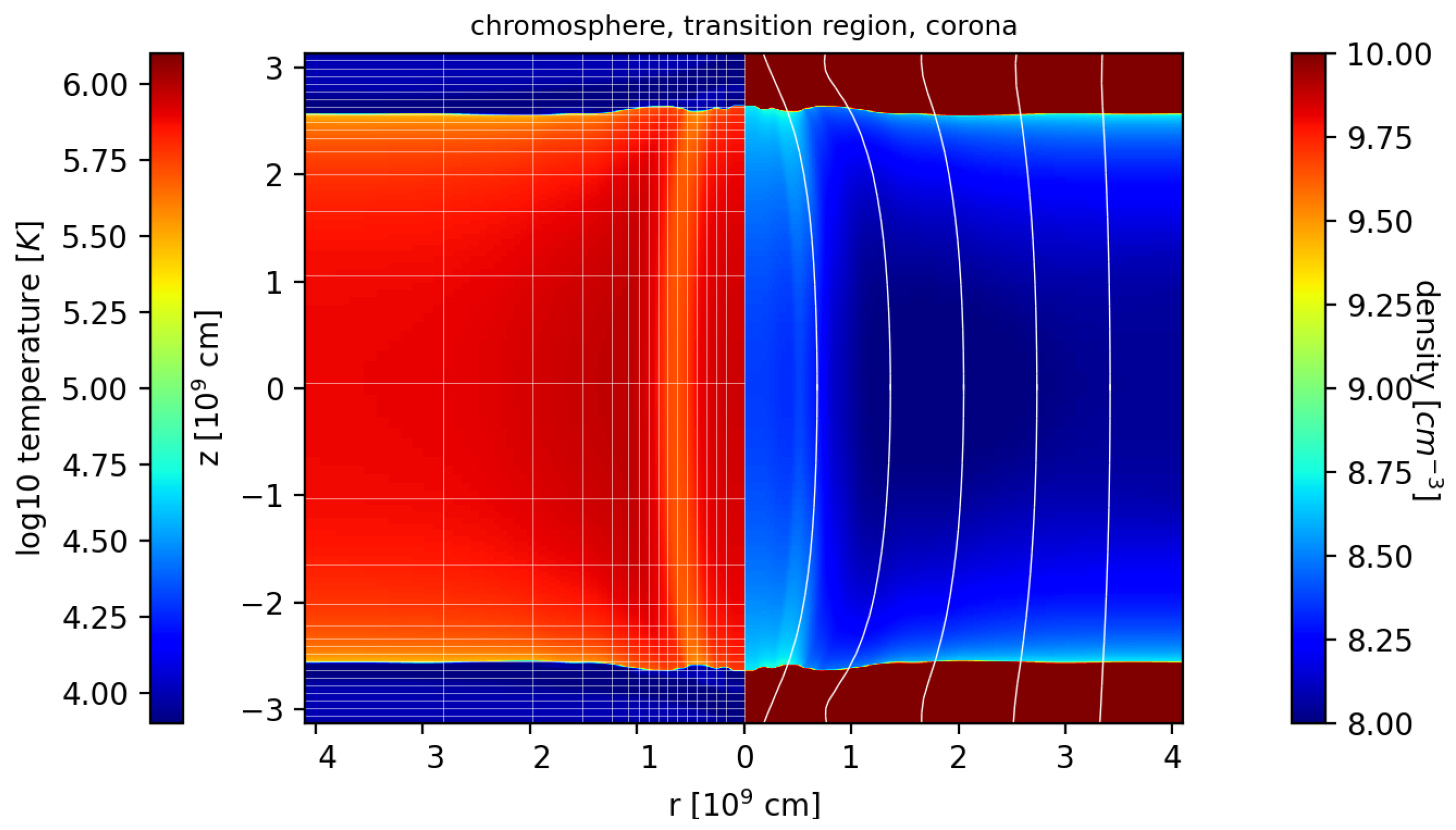
We considered a single, axi-symmetric coronal loop. The loop is modelled as a straightened magnetic flux tube hooked to two chromospheric layers at the opposite sides of the box. The length of the tube is much longer than its radius. For this reason, the effects of the curvature on its structure are negligible. Moreover, the two (upper and lower) chromospheric layers can be assumed as independent regions. The domain is a 2.5D box, while the geometry of the problem is cylindrical $(r,\varphi ,z)$. Plasma and magnetic fields evolve according to the full-time-dependent MHD equations. In particular, Equations (1)–(5) are solved inside the box, accounting for gravity in a semicircular loop, thermal conduction, heat flux saturation, optically thin radiative losses, and anomalous magnetic diffusivity.

The MHD equations are solved in the non-dimensional conservative form:

$$\frac{\partial \rho }{\partial t}+\nabla ·\left(\rho \mathbf{u}\right)=0,$$

(1)

$$\frac{\partial \rho \mathbf{u}}{\partial t}+\nabla ·(\rho \mathbf{uu}-\mathbf{BB}+\mathbf{I}{P}_t)=\rho \mathbf{g},$$

(2)

$$\frac{\partial \rho E}{\partial t}+\nabla ·\left[\mathbf{u}(\rho E+P_t)-\mathbf{B}(\mathbf{u}·\mathbf{B})\right]=\nabla ·\left[-\left(\frac{\eta }{c}\mathbf{J}\right)\times \mathbf{B}\right]+\rho \mathbf{u}·\mathbf{g}-\nabla ·{\mathbf{F}}_{\mathbf{c}}-n_e{n}_H\mathsf{\Lambda }\left(T\right)+Q,$$

(3)

$$\frac{\partial \mathbf{B}}{\partial t}+\nabla ·(\mathbf{uB}-\mathbf{Bu})=-\nabla \times (\eta ·\mathbf{J}),$$

(4)

$$\nabla ·\mathbf{B}=0;$$

(5)

and,

$$P_t=p+\frac{\mathbf{B}·\mathbf{B}}{2},$$

(6)

$$\mathbf{J}=c\nabla \times \mathbf{B},$$

(7)

$$E=ϵ+\frac{\mathbf{u}·\mathbf{u}}{2}+\frac{\mathbf{B}·\mathbf{B}}{2\rho },$$

(8)

$${\mathbf{F}}_{\mathbf{c}}=\frac{F_{sat}}{F_{sat}+\left|F_{class}\right|}{\mathbf{F}}_{\mathbf{class}},$$

(9)

$${\mathbf{F}}_{\mathbf{class}}=k_{\Vert }\widehat{\mathbf{b}}(\widehat{\mathbf{b}}·\nabla T)+k_{\perp }\left[\nabla T-\widehat{\mathbf{b}}(\widehat{\mathbf{b}}·\nabla T)\right],$$

(10)

$$|F_{class}|=\sqrt{{(\widehat{\mathbf{b}}·\nabla T)}^2(k_{\Vert }^2-k_{\perp }^2)+k_{\perp }^2\nabla T^2},$$

(11)

$$F_{sat}=5\rho c_{iso}^3,$$

(12)

where $P_t$ is the total pressure, $\mathbf{J}$ is the induced current density, and E is the total energy density (i.e., the sum of internal energy $ϵ$, kinetic energy, and magnetic energy). Moreover, t is the time, p is the thermal pressure, $n_e$ and $n_H$ are the electron and hydrogen number density, respectively, $m_H$ is the mass of hydrogen atom, $\mu =1.265$ is the mean atomic mass (assuming typical solar metal abundances, Anders & Grevesse 1989 [10]), $\rho$ is the mass density, $\mathbf{I}$ is the identity tensor, $\mathbf{B}$ is the magnetic field while $\widehat{\mathbf{b}}$ is the unit vector pointing along the magnetic field, $\eta$ is the magnetic diffusivity, $\mathbf{u}$ is the plasma velocity, $\mathbf{g}$ is the gravity acceleration vector for a curved loop, T is the temperature, ${\mathbf{F}}_{\mathbf{c}}$ is the thermal conductive flux (see Equations (9)–(12)), finally $k_{\Vert }=K_{\Vert }{T}^{\frac{5}{2}}$ and $k_{\perp }=K_{\perp }{\rho }^2/\left(B^2{T}^{\frac{1}{2}}\right)$ are the thermal conduction coefficients along and across the field respectively (where $K_{\Vert }=9.2\times {10}^{-7}$ and $K_{\perp }=5.4\times {10}^{-16}$ in cgs units). Classical thermal conductivity holds when the mean free path is relatively short. Vice-versa, when it becomes comparable to the temperature scale height, the heat flux is no longer equal to the classical values: we describe this effect as saturation. In this limit (i.e., for large temperature gradients), the flux is assumed independent from $\nabla T$. In particular, the flux magnitude approaches $F_{sat}=5\varphi \rho c_{iso}$, where $c_{iso}$ is the isothermal sound speed and $\varphi <1$ is a parameter we set to 0.9 (Cowie and McKee 1977 [11]). $\mathsf{\Lambda }\left(T\right)$ are the optically thin radiative losses per unit emission measure obtained from the CHIANTI v. 7.0 database (e.g., Dere et al., 1997 [12]; Reale et al., 2012 [13]; Landi et al., 2013 [14]) assuming typical coronal element abundances (Feldman 1992 [15]). $Q=4.3\times {10}^{-5}$ erg cm ${}^{-3}$ s${}^{-1}$ is a uniform heating rate per unit volume which maintains the corona with a temperature of about $8\times {10}^5$ K (Serio et al., 1981 [16], Rosner et al., 1978 [17]; Reale 2014 [1], Guarrasi et al., 2014 [9]). We use the ideal gas law, $p=(\gamma -1)\rho ϵ$ and assume negligible viscosity. Finally, the gravity in the corona can be treated by taking into account only the component along the tube. In this picture, the gravity acceleration decrease and becomes zero at the loop’s apex to model the loop curvature.

$$g\left(s\right)\widehat{\mathbf{s}}=g_{\odot }·sin\left(\frac{s}{R}\right),$$

(13)

where $g_{\odot }=\frac{G{M}_{\odot }}{R_{\odot }^2}$, G is the gravitational constant, $M_{\odot }$ is the solar mass, $R_{\odot }$ is the solar radius and $s=0$ corresponds to the loop’s apex.

By considering an anomalous plasma resistivity, ohmic dissipation activates only when the current density magnitude exceeds a certain threshold $J_{cr}$ (Hood et al., 2009 [7]):

$$\eta =\left\{\begin{array}{cc}\hfill {\eta }_0\hfill & \hfill \left|J\right|\ge J_{cr}\hfill \\ \hfill 0\hfill & \hfill \left|J\right|<J_c,\hfill \end{array}\right.$$

(14)

where we assume ${\eta }_0={10}^{14}$ cm, $J_{cr}=75$ Fr cm${}^{-3}$ s${}^{-1}$.

The calculations are performed using the PLUTO code (Mignone et al., 2007 [18], 2012 [19]), a modular, Godunov-type code for astrophysical plasmas (see Reale et al., 2016 [8] for more details about the numerical setup).

2.1. The Loop Setup

We addressed a typical active region loop of length $5\times {10}^9$ cm and initial temperature of ∼${10}^6$ K. The loop’s foot-points are anchored at the upper and lower boundaries of the domain through two independent chromospheric layers separated from the coronal environment by a steep transition region. Across this thin layer, temperatures suddenly increase from ${10}^4$ K, typical of the upper cromosphere, to a few million K in the corona. The magnetic field expands across the chromospheric layer as the plasma beta parameter decreases up to very small values in the corona. Such initial conditions are provided following the same procedure adopted in Guarrasi et al., 2014 [9]. Initially, the chromosphere and the corona are treated as two isothermal layers at temperatures of ${10}^4$ K and $8\times {10}^5$ K respectively. We assumed an initial vertical, non-uniform magnetic field. It is more intense near the axis ($B(r=0)\sim 500G$), and it decreases radially down to a background value of 10 Gauss. As we let this configuration relax, the magnetic field expands in the corona until a horizontal total pressure balance sets in. In contrast, below the transitions region, the magnetic field lines remain fundamentally unperturbed as they are rooted in the dense high-$\beta$ chromospheric plasma. Finally, in the longitudinal direction, density and temperature vary until thermal conduction, radiative losses and a background heating balance, and the loop relaxes to the steady state configuration described so far. In this new configuration, the magnetic field is more intense in the deep chromosphere, reaching 300 Gauss. It then degrees in the corona up to 12 Gauss at the loop apex.

The computational domain is 2.5 D cylindrical. The domain range is $-z_M<z<z_M$ (with $z_M=3.1\times {10}^9$ cm) in the vertical direction and $r_0\le r\le r_M$ (where $r_0=7\times {10}^7$ cm and $r_M=3.5\times {10}^9$ cm) in the radial direction. To properly account for the transition region, high spatial resolution is needed (Bradshaw & Cargill 2013 [20]). For this reason, the cell size in the corona decreases from $\left|z\right|\sim 2.4\times {10}^9$ cm to $dr\sim dz\sim 3\times {10}^6$ cm in the transition region. The adopted piece-ways uniform and stretched grid is sketched in Figure 1. We assume reflective boundary conditions (B.Cs.) near the symmetry axis (i.e., at $r=r_0$) and at $r=r_M$; periodic B.Cs. at the azimuthal boundaries; and equatorial-symmetric B.Cs. at $z=\pm z_M$.

2.2. Loop Twisting

We tested the evolution of a coronal loop under the effects of a footpoint rotation. Rotation at the loop’s foot-points induces a twisting of the magnetic field lines. As flux tube torsion proceeds, the current density is amplified and eventually exceeds a critical value triggering magnetic diffusion and heating via ohmic dissipation. Two rotation profiles have been taken into account. The first one is that of a rigid body around the central axis, i.e., the angular speed is constant in an inner circle and then decreases linearly in an outer annulus (Reale et al., 2016 [8]).

$$v_{\varphi }=\omega \left(r\right)r,$$

(15)

$$\omega =v_{max}/R_{max}\times \left\{\begin{array}{ll}1& r<R_{max}\\ (2R_{max}-r)/R_{max}& R_{max}<r<2R_{max}\\ 0& r>2R_{max},\end{array}\right.$$

(16)

where $v_{max}$ is the maximum tangential velocity and $R_{max}$ provides a size of the region subjected by photospheric rotation. The second one is a smoother profile (Reid et al., 2018 [21]) where the tangential velocity increases almost linearly around $r\sim 0$ cm and becomes zero for $r>2R_{max}$. The velocity decreases rapidly toward zero at $r\sim R_{max}$, but the profile is differentiable everywhere.

$$v_{\varphi }=\left\{\begin{array}{ll}2v_{max}\frac{r}{a}{(1-\frac{r^2}{a^2})}^3& r<a\\ 0& r\ge a,\end{array}\right.$$

(17)

where $a=2R_{max}$. The angular velocity profiles as a function of radius are sketched in Figure 2.

Five different configurations of $v_{max}$ and $R_{max}$ were explored. In cases a. and b., both foot-points are driven by a coherent photospheric rotation at the same speed and same radius. In case c., only one foot-point rotates under the influence of the photospheric boundary conditions. In case d. different dimensions of the rotation pattern at the loop basis are considered. In the last case, the loop initially evolves symmetrically as in cases a. and b. and, after a while ($t_0=1400$ s), one foot-point progressively slows down and stops (after $\delta =600$ s) while the other one accelerates up to 10 km/s as in configuration c. The time $t_0$ was chosen so that the loop is already filled by chromospheric plasma when the symmetry at the foot-points is broken. The choice of a photospheric rotation with a maximum tangential velocity of 10 km/s is a compromise to have effective heating in reasonable computational times while still maintaining a velocity in the order of realistic ones. In this work, we are exclusively interested in the coronal evolution of the flux tube; therefore, we make simplifying assumptions regarding the photosphere and the chromosphere, and we do not study their details.

3. Results

Our model presents a coronal loop that is straightened into a vertical magnetic flux tube hooked to two independent chromospheric layers. The magnetic field rapidly expands through the chromosphere while the loop body in the corona has an approximately constant cross-section. Figure 3 shows the initial condition of the simulation. It shows the steep gradient of the density ($\rho$) and temperature ($T)$ across the transition region and the strong change of plasma $\beta$ by a few orders of magnitude across the domain. The vertical component of the current density ($J_z$) is initially zero because the loop is untwisted. For completeness, the figure shows the null maps of angular velocity ($v_{\varphi }$). Finally, to track the plasma upward motions from the chromosphere, we also include the map of a passively-advected tracer of the chromospheric mass, initially identified where T < 10,000 K.

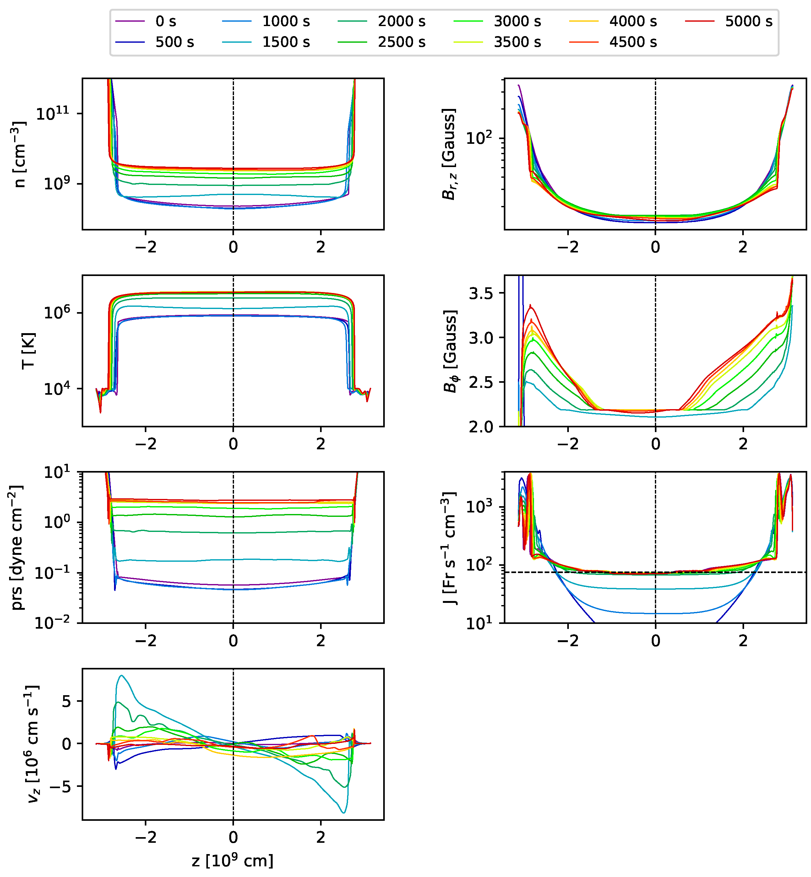
3.1. Mirror-Symmetric Driver

In simulations a. and b. (see

Table 1. The table shows the five cases explored to study the loop’s behaviour under different photospheric drivers. Each case differs for the maximum speed of the rotation ($v_{max}$) or its maximum extent ($r_{max}$). Moreover, two different profiles are considered (Reale et al., 2016 [8], Reid et al., 2018 [21]). Each foot-point undergoes an independent evolution. They are labelled as “up” and “down”.

Simulation	Down		Up
	${\mathit{v}}_{\mathit{max}}$ [km/s]	${\mathit{R}}_{\mathit{max}}$ [km]	${\mathit{v}}_{\mathit{max}}$ [km/s]	${\mathit{R}}_{\mathit{max}}$ [km]	Velocity Profile
a.	5	3000	5	3000	Reale et al., 2016
b.	5	3000	5	3000	Reid et al., 2018
c.	10	3000	0	*	Reale et al., 2016
d.	5	6000	5	1500	Reale et al., 2016
e. (for t < $t_0$)	5	3000	5	3000	Reale et al., 2016
e. (for $t>t_0+\delta$)	10	3000	0	*	Reale et al., 2016

* The radius is not defined because no rotation occurs.

), the rotation at both loop footpoints is driven by the same but opposite photospheric motions. Figure 4 and Figure 5 show the maps at $t=5000$ s for simulations a. and b., respectively.

At the very beginning, the rotation propels material just above the photospheric boundary. As the magnetic field is frozen into the plasma, this rotation generates an azimuthal component of the magnetic field which propagates as perturbation upward to the corona. The same happens to the azimuthal component of the velocity so that the loop is progressively twisted throughout. Figure 6 shows the sampled velocity of such magnetic perturbation travelling along the loop compared to the theoretical Alfvén velocity and the map of the Alfvén speed at t = 0 s. Of course, the propagation speed of the signal is slow in the dense chromosphere and greatly speeds up in the much more tenuous corona. The signal-travelling velocity agrees with what is expected from the theoretical value $v_{alf}=\frac{B}{\sqrt{4\pi \rho }}$.

The vertical component of current density also grows with the twisting. However, its sign reverses at a larger radial distance from the centre (i.e., outer ring) where the the radial derivative of the tangential velocity switches its sign (see Equations (16) and (17)). Since outside of the loop, no twisted magnetic field is present, according to Ampere’s law, the total current flowing across the loop must be zero. Thus, an inversion current is present in the outer shells of the loop as shown in Figure 4 and Figure 5. In the corona, the z-component of the current density dominates over the others. The current perpendicular to z is more concentrated below the transition region where the loop expansion is stronger. Current flows inside and outside of the domain across the upper and lower boundaries as a consequence of the boundary conditions.

In the sheared shell, between twisting and no twisting, there is some magnetic compression, which makes some dense plasma move upwards from the chromosphere. Indeed the chromosphere is more compressed by the twisting than the corona because the magnetic field is stronger there. As a consequence of that, the chromospheric plasma is forced to rise above the corona. By looking at the tracers in Figure 4 and Figure 5, we might conclude that the smoother the shearing layer, the slower this plasma transfer (Figure 2).

Indeed, the compression experienced by the tube is proportional to the gradient of the tension provided by the twisted magnetic field lines. There is stronger compression when the radial profile of the angular velocity is steeper. A stronger compression, in turn, drives more upflowing plasma. For this reason, the harsher the velocity profile, the more intense will be the ascended material across the outer boundary of the magnetic tube.

The current density first increases in the shell boundary layer between the twisted and untwisted region (i.e., at $r=6000$ Km ) (Reale et al., 2016). It takes some minutes to grow above the critical value in the corona and trigger the heating by ohmic dissipation. In particular, after 800 s, it exceeds the threshold of 75 Fr cm${}^{-3}$ s${}^{-1}$, and the enhanced resistivity allows magnetic dissipation to start in the corona and the gained magnetic energy is partially released as heating. The ohmic dissipation remains mostly localised just above the chromosphere, where the current density magnitude is higher, because of the tapering of the magnetic field. The density magnitude of the inversion current is close to the direct current in the corona but mostly below the dissipation threshold and, therefore, not driving significant plasma evaporation. Because of the efficient thermal conduction, the whole magnetic tube almost uniformly heats up to about 4 MK after $t=1500$ s in the central part of the tube, much less in the outer shell. The heating drives an overpressure which makes chromospheric plasma expand upwards to fill the tenuous coronal part of the tube (chromospheric evaporation). After $t=2400$ s, the coronal loop is filled by a dense and hot plasma and the initial, tenuous coronal plasma is compressed near the loop apex. The plasma is confined in the inner cylindrical region and a thin and more tenuous shell. In particular, inside the tube, the density increases up to ∼${10}^9$ cm${}^{-3}$ while in the outer shell, only to $3\times {10}^8$ cm${}^{-3}$. After $t=2400$ s, evaporation has slowed down, and the flow motion is significantly smaller. The evaporating chromospheric plasma moves upward following the orientation of the twisted magnetic field lines, as shown by the reversed-signed $v_{\varphi }$ component inside the flux tube and just above the chromosphere. The coronal part of the loop is not completely empty initially. For this reason, the chromospheric plasma flowing upwards cannot penetrate the preexisting coronal plasma and remains behind it, thus, filling the loop only partially and not reaching the loop apex.

Figure 7 shows the radial profiles of the density, temperature, pressure, magnetic field intensity, azimuthal component of the magnetic field, and current density at the top of the loop at different times. In the last panel of Figure 7, the velocity at the photospheric level is shown. The profiles are consistent with those in Reale et al., 2016 [8]. In particular, density, temperature, and pressure peak at the central axis. Then they decay to ambient values outside the tube cross-section. The secondary peak at $r\simeq 1.2\times {10}^9$ cm is localised in the outer shell, which is heated mostly by compression. Each quantity is only slightly perturbed by the twisting, and it is left almost unchanged until ohmic heating is switched on. As shown in Figure 7, Figure 8 and Figure 9, the azimuthal component of the magnetic field grows almost linearly in time, as expected from the ideal induction equation. Indeed, for a straight, cylindrical tube $\frac{\partial B_{\varphi }}{\partial t}=\frac{\partial \left(v_{\varphi }{B}_z\right)}{\partial z}$. Then, taking $v_{\varphi }\sim \omega \left(r\right)r\frac{z}{L}$ (we assume the absolute value of the angular velocity decreases almost linearly with height and becomes zero at the loop apex) and $B_z$ uniform along the whole tube’s length $2L$, we find: $B_{\varphi }=\frac{\omega \left(r\right)r{B}_z}{L}t$. During the last stages of the simulation, ohmic diffusion efficiently damps the rise of $B_{\varphi }$, which settles to a steady value. The radial profile of the azimuthal magnetic field fits, as expected, the shape of the implemented photospheric rotation. The rise of $B_{\varphi }$ influences the radial profile of the vertical magnetic field since it carries a stronger and stronger magnetic tension that compresses the inner twisted flux tube. For this reason, the vertical component of the magnetic field slightly rises up in a region close to the loop’s axis. On the other hand, since the magnetic field is line tied to the photosphere, magnetic flux is globally kept constant also in the corona. So, $B_z$ must drop just outside the region where magnetic twisting is performed to preserve the magnetic flux. The behaviour of $B_z$ found in these simulations fits the numerical solutions of the Grand–Shafranov equation retrieved in Browning & Hood 1989 [22].

Figure 8 shows the density, temperature, pressure, magnetic field intensity, azimuthal component of the magnetic field, and current density along the vertical direction and near the symmetry axis $r=0$ at different times. Because of the cylindrical symmetry of the problem (and the solenoidal condition $\nabla ·\mathbf{B}=0$), the magnetic field lines at $r=0$ are expected to be aligned with the axis. For this reason, we probed the physical properties of the plasma along a field line. Temperature, density and pressure do not change until heating starts at $t\simeq 800$ s. Then, the temperature suddenly rises and overcomes 3 MK at the end of the simulation. Pressure and density rise as well at a rate that can be traced by looking at the evolution of vertical velocity. In particular, the chromospheric plasma is accelerated in a very sharp region (the transition region) where the density abruptly drops with height. In a few ${10}^7$ cm, the velocity reaches values of several ${10}^6$ cm/s. Its maximum is placed just above the transition region. While climbing the thread, the material decelerates as it compresses the overlying plasma. At the loop apex, the velocity is zero, as expected from symmetry arguments. $B_z$ and $B_r$ magnetic field components do not seem to change by the twisting (at the list, near the loop axis). $B_{\varphi }$ and consequently, the magnitude of the current density grows fast at the beginning of the simulation as photospheric rotation twists the flux tube. Finally, at the end of the simulation, temperature, density, and pressure, as well as the $\varphi$ component of the magnetic field and current density magnitude, settle to a stable value as the magnetic diffusion balances the growing field stresses. Once again, the results found here are consistent with those shown in previous works (Guarrasi et al., 2014 [9], Reale et al., 2016 [8]) as well as with 1D hydrodynamics simulations (Warren 2002 [23]).

Figure 9 shows the trend of the maximum (black line) and averaged (red line) temperature, the maximum values of the vertical velocity, the maximum current density magnitude, the maximum and averaged heating rate and the temporal behaviour of the azimuthal component of the magnetic field in four different locations inside the domain. Space-averaging has been performed inside a cylinder of radius ${10}^9$ cm, entirely contained within the corona ($T>{10}^4$ K).

The maximum temperature and the averaged one (top left panel) are initially steady at about 1 MK. The maximum temperature increases at t = 800 s, and at the end of the simulation, it overcomes 3 MK, typical of an active region loop. The average temperature increases significantly only after 1300 s, and it reaches ≃2.5 MK after 3000 s. Loop heating is provided by the electric current density as soon as it exceeds the threshold of 75 Fr cm${}^{-3}$ s${}^{-1}$ after 800 s. The maximum vertical speed shows that the plasma evaporation also starts as soon as the maximum current magnitude exceeds the threshold for dissipation in the corona ($t\sim 800$ s). It peaks at t = 1500 s ($v_{max}\simeq 8\times {10}^6$ cm/s), approximately when the first impulsive evaporation front reaches the top of the loop, and then settles at ∼$6\times {10}^6$ cm/s indicating more gentle evaporation. These values are subsonic and usual for evaporation, driven by a continuous sequence of heat pulses (e.g., Patsourakos & Klimchuk 2006).

The maximum heating rate is shown in the upper panel on the right. The average heating rate is instead plotted in the middle panel on the right column. It is obtained by averaging only among the effectively heated cells, i.e., where $j\ge j_{cr}$. Both quantities keep growing as the squared value of the maximum (averaged) current density.

In the last panel of Figure 9, the azimuthal magnetic field component $B_{\varphi }$ is shown at two different heights (along the loop apex and just above the transition region) and two different radial distances from the central loop axis (close to the axis and 3000 km apart). The twisting initially makes $B_{\varphi }$ grow linearly at all positions. After t = 1200 s $B_{\varphi }$ stops growing close to the loop’s axis and to the chromosphere because of magnetic dissipation.

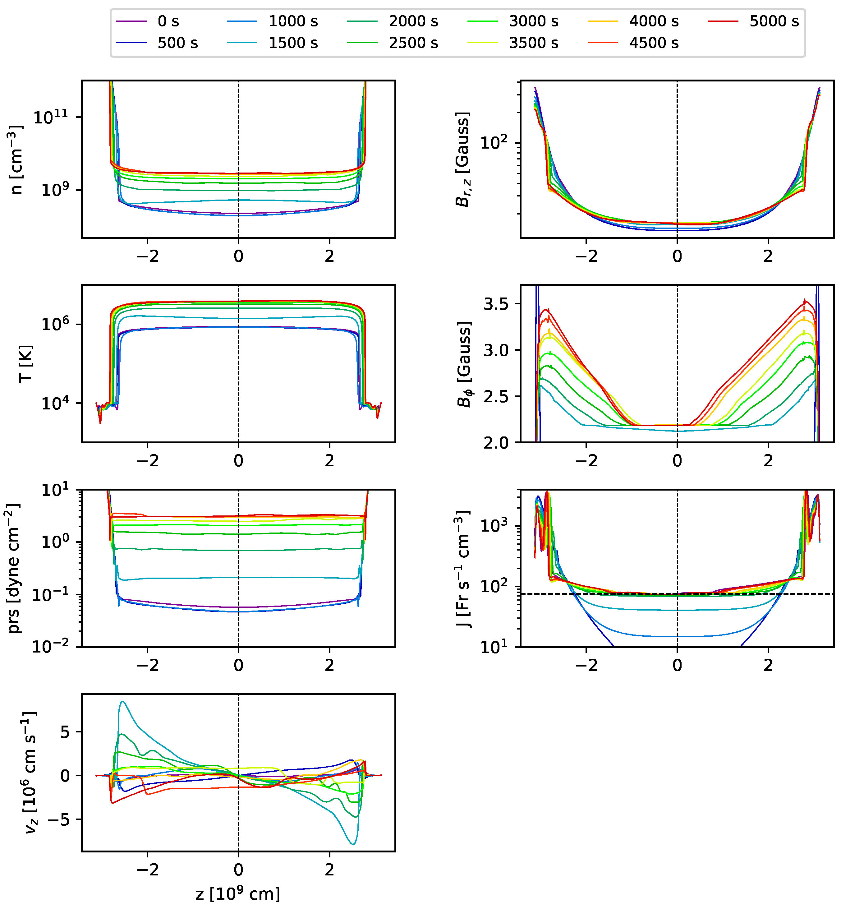
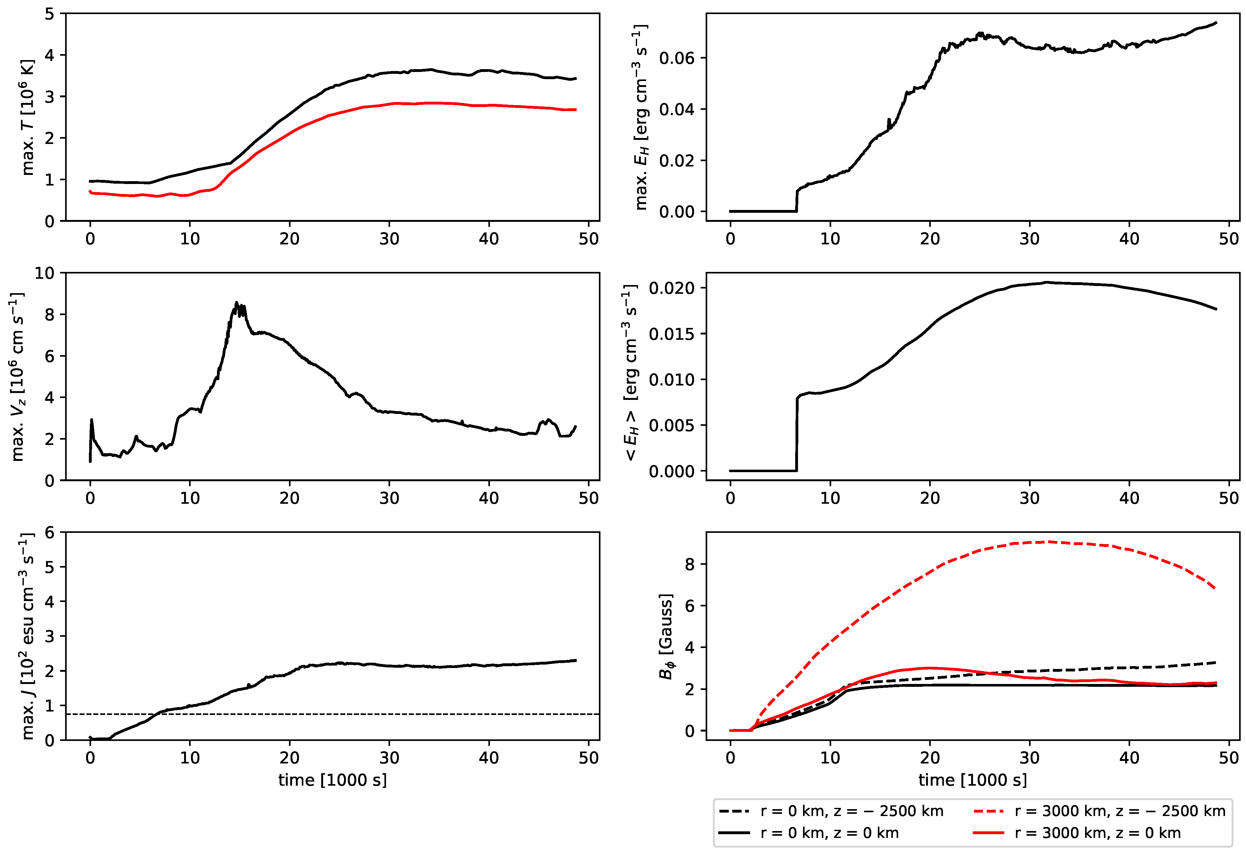
3.2. Asymmetric Twisting

We so far have discussed cases a. and b. where photospheric rotation is symmetric at the upper and lower boundary conditions, and the loop evolution is, therefore, mirror symmetric with respect to the loop apex. We now test how the symmetry of the coronal loop is retained upon the effect of an asymmetric driver. We consider three different cases, already described in Section 2.2 and listed in Table 1. In the case of c., one foot-point rotates while the other one is held fixed. In the case of d., both foot-points rotate at the same speed, but the rotation radius is different. Finally, in the case of e., the rotation begins symmetrically, but after a while ($t_0=1400$ s), one foot-point accelerates, and the other one slows down until it stops at $t_0+\delta =2000$ s. So in case e. asymmetries are implemented only after plasma evaporation has started filling the tube with dense chromospheric material.

3.2.1. Case c

In the case of c., one footpoint (the upper one) does not rotate; the other (lower) rotates at a speed twice bigger than in cases a. and b. so that the magnetic stress grows at the same rate. As in the previous experiments, rotation at the photospheric boundary twists the magnetic field lines. Initially, the twisting is localised near the rotating footpoint. Then, the azimuthal component of the magnetic field grows and propagates upwards, reaching the corona in the expected Alfvén time. Rotation never involves the upper chromospheric layer. Nevertheless, except for a certain time delay, the current density equally grows fast on both sides of the domain. It exceeds the threshold value after about 800 s, almost simultaneously in both upper and lower layers above the transition region. The loop evolution then continues very similarly to the symmetric cases for about 3800 s. Then the magnetic structure starts to warp. The final state of the simulation is shown in Figure 10. It represents the maps of density, temperature, azimuthal velocity, plasma beta, chromospheric tracer and current density at t = 5000 s. The dense, hot part of the loop fits the shape of the field lines. The azimuthal components of the plasma velocity are significantly higher where chromospheric evaporation fills the tube with dense material. There, the plasma $\beta$ is about one order of magnitude larger than in the surrounding environment because of the higher pressure, enhanced both by heating and compression. The tube expands on its lower half, and it is squeezed on the upper side. It is clearly visible, looking at the evolution of the tracer, that the upper-lying chromospheric material pushes down the underlying plasma. The same dynamics signature is visible in the orientation of the velocity in the r-z plane (black arrows in the third panel). This is because, on the upper side of the domain, more heating is released. Consequently, more plasma is injected from the upper side than the lower part. This is shown in the eighth panel of Figure 10. The dashed line in magenta encloses the region where the current density exceeds 75 Fr cm${}^{-3}$ s${}^{-1}$, i.e., where magnetic reconnection dissipates magnetic energy into heat. The heated region looks bigger on the upper side of the domain than in the lower part.

Figure 11 shows the density, temperature, pressure, magnetic field intensity, azimuthal component of the magnetic field, and current density probed along the vertical direction and near the symmetry axis at different times. During the first 2500 s, the loop’s evolution is closely symmetric. The profiles shown in Figure 11 are similar to those depicted in Figure 8. In the last 2500 s of the numerical experiment, temperature, density and pressure are only slightly evolved. For instance, the tube appears to warm up at slower and slower rates. The vertical velocity displays the same profile discussed before, but its peak decays in time as evidence of the reduced chromospheric evaporation. The height at which the velocity reverses its sign is not exactly the loop apex but displaced by a few hundred kilometres toward the lower part of the domain. Both the magnetic field components and the current density magnitude are clearly distorted from the mirror-symmetric initial configuration, and the asymmetry appears to grow in time.

Figure 12 shows the trend of the maximum (black line) and averaged (red line) temperatures, the maximum values of the vertical velocity, the maximum current density magnitude, the maximum and averaged heating rates, and the temporal behaviour of the azimuthal component of the magnetic field in six different locations inside the domain.

During the last 2500 s, the averaged and maximum temperatures reach a steady state, at 2.5 MK and 3.5 MK, respectively. As before, after the peak at t = 1600 s, the maximum velocity slowly decays to settle at about 20 km/s. Both the maximum current density and the maximum heating rate settle to about 250 Fr cm${}^{-3}$ s${}^{-2}$ and 0.07 erg cm${}^{-3}$ s${}^{-2}$, respectively, during the second half of the simulation. The average heating rate instead begins to decrease after t = 3000 s. The evolution of the azimuthal magnetic field at different locations along the flux tube (last panel of Figure 12) clearly shows the departure from mirror symmetry. As with the symmetric twisting, the azimuthal magnetic field initially increases everywhere but more rapidly, far from the axis where the tangential speed is faster. At $t\sim 1200$ s, the heating rate begins to grow, and at the same time, $B_{\varphi }$ saturates close to the loop axis, where the dissipation is stronger. Farther from the axis and at the loop apex, the magnetic field saturates slightly later. Finally, closer to the chromosphere but far from the axis, the azimuthal component keeps increasing with a trend very similar to the heating rate (dashed line) at z = $-2.5\times {10}^9$ cm, and a flat one (dotted line) at the opposite side, until the end of the simulation. The red dashed and dotted field lines remarkably depart in the final stages of the numerical experiment as a consequence of the broken mirror symmetry. The black dashed and dotted lines keep following the same path until the end of the simulation, suggesting that asymmetries become less pronounced near the loop axis.

3.2.2. Case d

In case d, both foot-points rotate around the symmetry axis at the same maximum tangential velocity $v_{max}$ but with a different extension of the rotating region for the footpoints ($R_{max}$). The smaller rotating footpoints rotate with faster angular velocity ($\omega =v_{max}/R_{max}$), as the paremeter $v_{max}$, is the same for both. Once again, the loop initially evolves very symmetrically, and its behaviour fits quite well with cases a and b, discussed in the previous section. As in case c., the effects of the asymmetric boundary conditions become dominant after 3800 s. Figure 13 shows the evolved coronal loop at $t=5000$ s. Figure 14 focus on the temporal evolution of several physical quantities sampled along the loop axis. Figure 15 finally displays the evolution in time of some maximum and space-averaged quantities. All the results shown in the previous figures agree very much with those shown in Figure 10, Figure 11 and Figure 12 for case c. Indeed, in both cases, asymmetries develop after 3000 s. In particular, the upper side of the loop is squeezed while the lower side of the structure expands. Since velocities and magnetic field strength at the photospheric boundaries are similar to case c., we expected to probe a similar evolution (at least in terms of times scales and orders of magnitude involved).

3.2.3. Case e

With case e., we wanted to test the behaviour of a coronal loop when asymmetries are implemented at the boundaries only after the flux tube has been filled by chromospheric plasma. Indeed, in the previous cases, asymmetric boundary conditions act from the beginning, i.e., when the magnetic structure encloses only a tenuous coronal atmosphere. This time, the flux tube initially evolves under the effect of a symmetric photospheric driver. After 1400 s, the lower foot-point accelerates to double its initial velocity. In the meantime, the upper foot-point progressively decelerates, and it stops after 2000 s. After that time, boundary conditions are the same as in case c. The initial evolution of the loop is exactly the same as in case a. (we performed the simulation deploying the rotation pattern described in Equations (15) and (16)). Moreover, in this case, asymmetries become clearly appreciable only after 3800 s from the beginning of the numerical experiment.

Moreover, in this case, the asymmetric evolution of the loop in the latest stages of the simulation remarks very well that described for case c. In particular, Figure 16 shows the evolved coronal loop at $t=5000$ s. Figure 17 focus on the temporal evolution of several physical quantities sampled along the loop axis. Figure 18 finally displays the evolution in time of some maximum and space-averaged quantities. All the results shown in the previous figures agree very much which those shown in Figure 10, Figure 11 and Figure 12 for case c. This is expected since, after 2000 s, the loop twisting is driven by the same photospheric driver considered for case c.

4. Discussion

We have addressed the brightening of a coronal loop hooked to two independent chromospheric layers through their footpoints. We performed a series of 2.5D simulations in cylindrical geometry. The coronal loop is treated as a straightened, cylindrically symmetric flux tube, where the gravity is that of a curved arch.

The basic assumption is that the flux tube is progressively twisted by the rotation of the footpoints due to photospheric motions. The tube is then heated by ohmic dissipation when the induced current grows above a threshold. Since it is difficult to imagine that the photospheric rotation is exactly identical at the two footpoints, here we study the effect of asymmetric twisting on the evolution of the heated loop. This extends the results presented in Reale et al., 2016 where only coherent photospheric motions are taken into account.

We chose to take into account five particular cases to explore the space of the parameters involved in the prescription of the photospheric rotation. For comparison, we first consider mirror-symmetric twisting in cases a. and b. which differ only for the radial shape of the angular velocity $\omega \left(r\right)$: trapezium-like vs smoother and everywhere differentiable, respectively. In particular, simulations a. and b. resemble the numerical experiments performed in the previous work (Reale et al., 2016). We ensure the new results are coherent with the older ones.

In case c., the rotation is driven only at one side of the cylindrical box; in case d., the rotating area is different from one footpoint to the other, maintaining the same maximum speed; in case e., the rotation is mirror symmetric initially and then made different after few thousands of seconds. In the last three cases, the loop evolution is closely symmetric for the first 3800 s. Asymmetries become non-negligible after the tube has been filled enough by dense chromospheric plasma.

All the simulation shows the same qualitative behaviour during the first 2400 s. The azimuthal component of the magnetic field and the current density are tracers of the degree of twisting of the magnetic field lines. Both quantities grow smoothly with the boundary rotation. Photospheric rotation is transmitted by the line-tied magnetic field up to the chromosphere and the corona at the expected Alfvén crossing time (see Figure 6). A quasi-steady coherent twisting settles in the corona after just a few Alfvén crossing travel times. Then, both the azimuthal component magnetic field and the maximum current amplitude grow almost linearly with time, as expected from the induction equation (Equation (4)). Energy is gained by the stressed magnetic field until the current density exceeds the threshold of 75 Fr cm${}^{-3}$ s${}^{-1}$. Then ohmic dissipation of the magnetic field is triggered, and the next evolution is similar to that found in previous loop models.

Here our attention focuses on the symmetry of evolution. We invariably observe that even when the rotation pattern at the footpoints is not symmetric (cases c., d., and e.), the evolution is initially symmetric, i.e., the evolution of the two legs of the tube almost overlaps. The explanation lies in the speed of propagation of the signal from one footpoint to the other. The magnetic twisting driven by the footpoint rotation is transmitted along the tube at the Alfvén speed. This speed is very high in the tenuous initial loop corona ($<v_{alf}>\sim 6\times {10}^7$ cm s${}^{-1}$) and makes the twisting uniform along the whole loop in a very short time (few Alfvén crossing travel times) and leads to the initially symmetric evolution. The chromospheric evaporation determines a reduction of the Alfvén speed and a slight disequilibrium which makes the heating more effective at first in the lower leg than in the upper one. The higher plasma pressure inflates the loop more, i.e., the magnetic field becomes weaker, and the current density as well, thus, eventually making the heating steadily weaker in the low region than in the upper region. A simple model can qualitatively describe the behaviour of the Alfvén velocity at the early stages of the simulation and the latest. Initially, the Alfvén speed grows slightly. Indeed, changes in the average magnetic field are relatively small (≤25%), and the density stays approximately constant for the first 1500 s. In particular, $B_{\varphi }$ grows almost linearly with time while $B_z$ and $B_r$ slightly readjust due to the rising azimuthal stresses. The evolution of $B_{\varphi }$ is approximately given by solving the induction equation, assuming that $B_r$ is negligible in the corona and $B_z$ can be kept constant throughout the initial part of the evolution. A simple expression for the Alfvén velocity follows from the previous assumptions:

$$v_A=\frac{B}{\sqrt{4\pi \rho }}\sim \frac{\sqrt{B_z^2+B_{\varphi }^2}}{\sqrt{4\pi \rho }}\sim \frac{B_z}{\sqrt{4\pi {\rho }_0}}\left[1+\frac{1}{2}{\left(\frac{\omega rt}{L}\right)}^2\right].$$

(18)

All three components lose strength because of ohmic dissipation at later times. In particular, after 2400 s, the strong current dissipation stops the growth of $B_{\varphi }$, which settles to a steady value. At the same time, the coronal density increases strongly because of chromospheric evaporation and reduces the Alfvén speed:

$$v_A\sim \frac{\langle B\rangle }{\sqrt{4\pi \rho \left(t\right)}}\propto \frac{1}{\sqrt{t}},$$

(19)

where $\langle B\rangle$ is the averaged magnetic field. The left panel of Figure 19 shows the evolution of the Alfvén speeds obtained by averaging over the pixels inside the coronal part of the flux tube (i.e., at $T>{10}^4$ K). It initially increases linearly. After 1000 s, it reaches a peak and then starts to decrease rapidly because of the increase in the plasma density.

To track the evolution of the asymmetries inside the loop, we consider a single magnetic field line at the edge of the flux tube, marked in Figure 20. We select two points along this field line at symmetric distances from the footpoints, and we measure their radial distance from the tube’s central axis as a function of time. This distance holds the same for mirror-symmetric simulations, but it does not if there are deviations from symmetry; so we are measuring these deviations, and we do this for all three simulations c., d., and e.

The middle and right panels of Figure 20 clearly show that for all three simulations, the general trend is that the distance is constant for about 2000 s, then it shrinks until a time between t = 3500 s and t = 4500 s, and widens again afterwards, showing a clear minimum. However, on all three simulations, the distance decreases much more for the lower point than for the other, and this detachment starts at $t\sim 2500$ s, thus, remarking the asymmetry since then.

Figure 21 shows the evolution of the plasma $\beta$ over time. It increases in the corona due to magnetic dissipation and further chromospheric evaporation. Asymmetries shown in the previous figure occur once the plasma beta has reached relatively high values in the corona. These results suggest that the asymmetries are allowed to occur only in relatively high-$\beta$ environments. In other words, the detachment from mirror-symmetry is not directly caused by the long-lasting nature of the asymmetric twisting but by its occurrence when the loop density is very high. Indeed, until the loop is not filled with dense plasma, asymmetries can not occur, not even if the foot-points have been dragged for a long time. On the other hand, a relatively rapid evolution of the asymmetries is expected in high beta coronal loops (as in case-e loop at time t = 2000 s).

5. Conclusions

We have extended the study done by Reale et al., 2016 by addressing a coronal loop twisted by asymmetric photospheric motions. Indeed, the previous work addressed a straightened coronal loop subjected to a symmetric twisting at its footpoints. This time, we consider that independent photospheric motions can drag field lines toward a stressed configuration. We, in particular, investigated the response of these coronal loops to non-coherent photospheric motions by forcing strong asymmetries at the boundary conditions. Our numerical MHD simulations show that coronal loops can maintain a very high degree of symmetry for a relatively long time against asymmetric twisting drivers at their footpoints.

Observations agree with the simulations. As far as isolated coronal loops are concerned, such magnetic flux tubes do not display strong side-by-side asymmetries despite their footpoints are likely driven by different rotation drivers at the photospheric footpoints. Here we only account for coherent drivers, but irregular patterns on smaller scales may lead to field braiding, making any possible asymmetry unobservable on large scales.

In general, the magnetically complex environment in which all coronal loops are embedded can influence each tube’s shape. For instance, coronal loops can be tangled with each other or may interact with open-field-lines structures. On the other hand, their cross-sections are widely observed to be almost constant along their length, i.e., they would appear symmetric if stretched. In other words, also non-isolated coronal loops possess a hidden symmetry that may be highlighted by looking at the uniformity of their physical properties (for instance, temperature, density, and emission measure) along their entire length. A plasma $\beta$ in the corona even smaller than the one implied by our model assumptions could explain why such coronal loops preserve so well such symmetry properties. Moreover, we understand that to break the symmetry, high plasma beta values are required. These regimes can be reached by long-lasting photospheric twisting. They are unlikely to occur because of the stochastic (turbulent) behaviour of the photospheric plasma. In addition, highly twisted coronal loops would be unstable against kink modes.

References

1. Reale, F. Coronal loops: Observations and modeling of confined plasma. Living Rev. Sol. Phys. 2014, 11, 1–94. [Google Scholar] [CrossRef] [PubMed] [Green Version]
2. Yang, Z.; Bethge, C.; Tian, H.; Tomczyk, S.; Morton, R.; Del Zanna, G.; McIntosh, S.W.; Karak, B.B.; Gibson, S.; Samanta, T.; et al. Global maps of the magnetic field in the solar corona. Science 2020, 369, 694–697. [Google Scholar] [CrossRef] [PubMed]
3. Long, D.M.; Valori, G.; Pérez-Suárez, D.; Morton, R.J.; Vásquez, A.M. Measuring the magnetic field of a trans-equatorial loop system using coronal seismology. Astron. Astrophys. 2017, 603, A101. [Google Scholar] [CrossRef] [Green Version]
4. Parker, E.N. Nanoflares and the solar X-ray corona. Astrophys. J. 1988, 330, 474–479. [Google Scholar] [CrossRef]
5. Ishikawa, R.; Bueno, J.T.; del Pino Alemán, T.; Okamoto, T.J.; McKenzie, D.E.; Auchère, F.; Kano, R.; Song, D.; Yoshida, M.; Rachmeler, L.A.; et al. Mapping solar magnetic fields from the photosphere to the base of the corona. Sci. Adv. 2021, 7, eabe8406. [Google Scholar] [CrossRef]
6. Gabriel, A. A magnetic model of the solar transition region. In Philosophical Transactions for the Royal Society of London. Series A, Mathematical and Physical Sciences; Royal Society: London, UK, 1976; pp. 339–352. [Google Scholar]
7. Hood, A.; Browning, P.; Van der Linden, R. Coronal heating by magnetic reconnection in loops with zero net current. Astron. Astrophys. 2009, 506, 913–925. [Google Scholar] [CrossRef]
8. Reale, F.; Orlando, S.; Guarrasi, M.; Mignone, A.; Peres, G.; Hood, A.; Priest, E. 3D MHD modeling of twisted coronal loops. Astrophys. J. 2016, 830, 21. [Google Scholar] [CrossRef]
9. Guarrasi, M.; Reale, F.; Orlando, S.; Mignone, A.; Klimchuk, J. MHD modeling of coronal loops: The transition region throat. Astron. Astrophys. 2014, 564, A48. [Google Scholar] [CrossRef] [Green Version]
10. Anders, E.; Grevesse, N. Abundances of the elements: Meteoritic and solar. Geochim. Cosmochim. Acta 1989, 53, 197–214. [Google Scholar] [CrossRef]
11. Cowie, L.L.; Mckee, C.F. The evaporation of spherical clouds in a hot gas. I-Classical and saturated mass loss rates. Astrophys. J. 1977, 211, 135–146. [Google Scholar] [CrossRef]
12. Dere, K.; Landi, E.; Mason, H.; Fossi, B.M.; Young, P. CHIANTI—An atomic database for emission lines-I. Wavelengths greater than 50 Å. Astron. Astrophys. Suppl. Ser. 1997, 125, 149–173. [Google Scholar] [CrossRef] [Green Version]
13. Reale, F.; Landi, E. The role of radiative losses in the late evolution of pulse-heated coronal loops/strands. Astron. Astrophys. 2012, 543, A90. [Google Scholar] [CrossRef] [Green Version]
14. Landi, E.; Reale, F. Prominence plasma diagnostics through extreme-ultraviolet absorption. Astrophys. J. 2013, 772, 71. [Google Scholar] [CrossRef] [Green Version]
15. Widing, K.; Feldman, U. Element abundances and plasma properties in a coronal polar plume. Astrophys. J. 1992, 392, 715–721. [Google Scholar] [CrossRef]
16. Serio, S.; Peres, G.; Vaiana, G.; Golub, L.; Rosner, R. Closed coronal structures. II-Generalized hydrostatic model. Astrophys. J. 1981, 243, 288–300. [Google Scholar] [CrossRef]
17. Rosner, R.; Tucker, W.H.; Vaiana, G. Dynamics of the quiescent solar corona. Astrophys. J. 1978, 220, 643–645. [Google Scholar] [CrossRef]
18. Mignone, A.; Bodo, G.; Massaglia, S.; Matsakos, T.; Tesileanu, O.E.; Zanni, C.; Ferrari, A. PLUTO: A numerical code for computational astrophysics. Astrophys. J. Suppl. Ser. 2007, 170, 228. [Google Scholar] [CrossRef] [Green Version]
19. Mignone, A.; Flock, M.; Stute, M.; Kolb, S.; Muscianisi, G. A conservative orbital advection scheme for simulations of magnetized shear flows with the PLUTO code. Astron. Astrophys. 2012, 545, A152. [Google Scholar] [CrossRef] [Green Version]
20. Bradshaw, S.J.; Cargill, P.J. The influence of numerical resolution on coronal density in hydrodynamic models of impulsive heating. Astrophys. J. 2013, 770, 12. [Google Scholar] [CrossRef] [Green Version]
21. Reid, J.; Hood, A.W.; Parnell, C.E.; Browning, P.; Cargill, P. Coronal energy release by MHD avalanches: Continuous driving. Astron. Astrophys. 2018, 615, A84. [Google Scholar] [CrossRef] [Green Version]
22. Browning, P.; Hood, A. The shape of twisted, line-tied coronal loops. Sol. Phys. 1989, 124, 271–288. [Google Scholar] [CrossRef]
23. Warren, H.P.; Winebarger, A.R.; Hamilton, P.S. Hydrodynamic modeling of active region loops. Astrophys. J. 2002, 579, L41. [Google Scholar] [CrossRef] [Green Version]
Figure 1. Maps of initial temperature (left) and density (right) distributions. For instance, cold colours on the left represent the chromospheric layer, where temperatures do not exceed 10 thousand kelvins. Shades of red instead colour the nearby 1M K hot coronal environment. Chromosphere and corona are separated by a steep transition region where high gradients of temperature and density occur. On the left, straight white lines highlight the structure of the non-uniform grid. A higher resolution is expected across the chromospheric layer and the transition region as well as in the highest magnetised regions of the domain (i.e., near the loop’s axis). On the right, solid, white lines trace the shape of the magnetic field. Magnetic field expansion (tapering) is clearly visible at the top and bottom sides of the flux tube.
Symmetry 15 00627 g001
Figure 2. The solid and dashed, black lines represent the profiles of two angular velocities implemented at the lower and upper boundaries of the domain. In the first case (solid line), the photosphere initially ( r R m a x ) rotates as a solid body. Then (for r > R m a x ), it linearly decays to zero. There are two discontinuities in the derivative of ω ( r ) at r = R m a x and at r = 0 . For r > 2 R m a x , there is no rotation. In the second case (dashed line), the angular velocity profile is smoother: it is everywhere differentiable. Again, the rotation kindly stops at r > 2 R m a x .
Symmetry 15 00627 g002
Figure 3. First row: maps of the initial plasma density, temperature, azimuthal velocity, and tracer. Second row: maps of the initial plasma beta, azimuthal magnetic field, magnetic field magnitude on the r-z plane, and vertical component of the current density. Field lines are marked as solid white lines. Initial conditions are the same for all the simulations discussed below. Black lines in the last panel enclose the region of the domain where T > 10 4 K (i.e., transition region and corona).
Symmetry 15 00627 g003
Figure 4. Same as Figure 3 for Simulation a. and after 5000 s. The black arrows in the third panel show the orientation of the plasma velocity along the r-z plane. The dashed line in magenta in the last panel encloses the region of the domain where the current density exceeds the current threshold of 75 Fr cm 3 s 1 .
Symmetry 15 00627 g004
Figure 5. Same as Figure 4 for Simulation b.
Symmetry 15 00627 g005
Figure 6. (Left): theoretical Alfvén velocity (solid line) progresses upwards along the central z-axis, as compared to the velocity of the signal propagating at a certain height and measured in the simulation (dashed line). (Right): map of the Alfvén velocity at t = 0 s. The logarithmic colour scale emphasizes the deep difference in magnitude between the chromosphere and corona.
Symmetry 15 00627 g006
Figure 7. (Simulation a.) First column: radial profiles of density, temperature, pressure at z = 0 (loop apex) and velocity at the photospheric level. Second column: total magnetic field intensity, azimuthal component of the magnetic field and modulus of the current density. The profiles are spaced by about 200 s, and the colour coding marks the time progression from purple (0 s) to red (5000 s).
Symmetry 15 00627 g007
Figure 8. (Simulation a.) First column: vertical profiles of density, temperature, pressure and velocity at r 0 (near the loop axis). Second column: vertical profiles of the total magnetic field intensity, azimuthal component of the magnetic field and modulus of the current density at r 0 (near the loop axis). The profiles are spaced by 500 s, and the colour coding marks the time progression from purple (0 s) to red (5000 s). In the third panel on the right, the critical current density is marked by a horizontal dashed line.
Symmetry 15 00627 g008
Figure 9. (Simulation a.) Evolution of the maximum temperature, vertical velocity, and coronal maximum current density in the simulation domain, and of the maximum heating rate per unit volume (top), the averaged heating over cells with E h > 0 , and of the azimuthal component of the magnetic field B ϕ , at the two labelled heights z along the loop, i.e., apex (solid) and just above the transition region (dashed) and at the two labelled radial distances r from the central axis, i.e., close to the axis (black) and 3000 km far away (red). In the left panel, the averaged temperature (red line) and current threshold for dissipation (horizontal dashed line) are also shown. Space-averaging is performed inside a cylinder of radius 10 9 cm, entirely contained within the corona (T > 10 4 K).
Symmetry 15 00627 g009
Figure 10. Same as Figure 4 for Simulation c.
Symmetry 15 00627 g010
Figure 11. Same as Figure 8 for Simulation c.
Symmetry 15 00627 g011
Figure 12. Same as Figure 9 for Simulation c. We represented in the last panel (bottom left) the azimuthal component of the magnetic field B ϕ at the three labelled heights z along the loop, i.e., apex (solid) and just above the transition region z = 2.5 × 10 9 cm (dashed) and z = 2.5 × 10 9 cm (dotted) and at the two labelled radial distances r from the central axis, i.e., close to the axis (black) and 3000 km far away (red). The current threshold for dissipation (horizontal dashed line) is also shown. Space-averaging is performed inside a cylinder of radius 10 9 cm, entirely contained within the corona (T > 10 4 K).
Symmetry 15 00627 g012
Figure 13. Same as Figure 4 for Simulation d.
Symmetry 15 00627 g013
Figure 14. Same as Figure 8 for Simulation d.
Symmetry 15 00627 g014
Figure 15. Same as Figure 12 for Simulation d.
Symmetry 15 00627 g015
Figure 16. Same as Figure 4 for Simulation e.
Symmetry 15 00627 g016
Figure 17. Same as Figure 8 for Simulation e.
Symmetry 15 00627 g017
Figure 18. Same as Figure 12 for Simulation e.
Symmetry 15 00627 g018
Figure 19. Evolution of the pixel-averaged Alfvén velocity v A l f (left). magnetic field B (middle), and density ρ (right). Black, red, and blue lines refer, respectively, to models c, d, and e. Space-averaging is performed inside a cylinder of radius 10 9 cm, entirely contained within the corona (T > 10 4 K).
Symmetry 15 00627 g019
Figure 20. (Left): Map of the density at time t = 3500 s with field lines for simulation c. We selected a specific field line (solid blue line) and two symmetric points along it (red points), and we measured their distance r u p and r d o w n from the axis (red lines). (Middle): r u p and r d o w n vs time for cases c., d., and e. (Right): difference Δ r = r u p r d o w n vs time for cases c., d., and e. Black, red, and blue lines refer, respectively, to models c, d, and e.
Symmetry 15 00627 g020
Figure 21. Evolution of the pixel-averaged plasma b e t a . Black, red, and blues lines refer, respectively, to models c, d, and e. Space-averaging is performed inside a cylinder of radius 10 9 cm, entirely contained within the corona (T > 10 4 K).
Symmetry 15 00627 g021