Numerical Method for Solving Fractional Order Optimal Control Problems with Free and Non-Free Terminal Time

Abstract

The optimal control theory in mathematics aims to study the finding of control for a dynamic system over time, where an objective function is optimized. It has a broad range of applications in engineering, operations research, and science. The main purpose of this study is to provide numerical algorithms for two cases of optimal control problems of fractional order that involve fractional order derivatives with free and non-free terminal time. In addition to comparing the numerical results for three test problems with exact solutions of these problems, various computer simulations are also introduced.

1. Introduction

Optimal control is the study of finding a dynamic control system over time in order to optimize an objective function. It has many uses in operations research, engineering, and science. For instance, the dynamic system could be a spacecraft with controls that correspond to rocket thrusters, and the goal could be to reach the moon using the least amount of fuel. In terms of result, the dynamic system could be a country’s economy with the goal to minimize unemployment; in this scenario, the controls could be fiscal and monetary policy. It is also possible to integrate operations research issues into the framework of optimal control theory by using a dynamic system. Additionally, a branch of mathematics and physics known as the fractional dynamics examines how objects and systems behave by differentiating fractional orders. Research on fractional dynamical systems has produced novel findings that have attracted the interest of a significant audience of professionals, including mathematicians, physicists, applied researchers, and practitioners. This is due to the topic’s wide applications in science and technology. In contrast to integer-order models, however, fractional-order models offer the potential to express non-local relations in time and space using power law memory kernels [1]. Consequently, this indicates that they offer more accurate and more realistic results. Moreover, the standard integral and differential calculus are generalized to any order in fractional calculus. If the order of the fractional derivative operator is an integer m, we obtain an m-fold integral when m is negative and the traditional derivative of order m when m is positive. Furthermore, for the review of the literature on numerical studies of fractional optimal control problems (FOCPs), Agrawal [2] preformed a formulation and numerical scheme for FOCPs, the work in [3] introduced the numerical solution of some types of FOCPs, while Bhrawy et al. [4] introduced an accurate numerical technique for solving FOCPs. Furthermore, a new method for the numerical solution of FOCPs was introduced in [5]. Furthermore, to solve multidimensional FOCPs with a quadratic performance index, the authors of [6] developed a practical numerical method for the purpose of solving FOCPs, and Doha et al. [7] investigated an effective numerical method based on the shifted orthonormal Jacobi polynomials. However, the generalized differential transform approach was used in [8] to introduce the numerical solutions of the coupled space-and-time Burgers equations. Lotfi et al. [9] introduced a numerical technique for solving FOCPs, Pooseh et al. [10] introduced a numerical scheme to solve FOCPs, Zhao and Li [11] solved the time–space fractional telegraph equation using the fractional difference-finite element, and Mechee and Senu [12] studied the numerical solution of fractional differential equations of Lane–Emden type by the method of collocation. For the space fractional diffusion equations, Zhou et al. [13] studied the quasi-compact finite difference schemes, and Bhrawy et al. [14] investigated a new Jacobi spectral collocation approach for fractional coupled Schrödinger systems and 1 + 1 fractional Schrödinger equations. At the same time, for the review of the literature on Legendre polynomials, using a Chebyshev–Legendre operational technique, Bhrawy et al. [15] solved the fractional optimal control for dynamical systems problems (FOCDSs). In fact, Yousefi et al. [16] employed a Legendre multiwavelet collocation approach in order to solve the FOCPs. In contrast, Bhrawy and Ezz-Eldien [17] used a new Legendre operational technique for solving delay FOCPs, in similar to Dirichlet boundary conditions, Heydari et al. [18] solved fractional partial differential equations (FPDEs) using the Legendre wavelets method. On the other hand, for the solution of fractional sub-diffusion and reaction sub-diffusion equations, Doha et al. [7] utilized an effective Legendre spectral tau matrix formulation, Khan and Khalil [19] provided a new approach that is based on Legendre polynomials. In parallel to these researchers, Sweilam and Al-Ajami [20] solved some types of FOCPs using the Legendre spectral-collocation method; additionally, some authors studied different cases of fractional differential equations. To solve the space fractional order diffusion equation, Sweilam et al. [21] utilized the second sort of shifted Chebyshev polynomials, but a discrete method for solving FOCPs was introduced in [22], while ref. [23] established a fractional adaptation strategy for lateral control of an AGV; whereas, Pinto and Tenreiro Machado [24] introduced the fractional dynamics of computer virus propagation, Pooseh et al. [25] studied the FOCPs with free terminal time by using operational matrices of Bernstein polynomials, Jafari and Tajadodi [26] solved the FOCPs, and Jesus and Tenreiro Machado [27] investigated the fractional control of heat diffusion systems. Thereafter, for a review of more literature on the applications, Ahmad and El-Khazali [28] introduced the fractional-order dynamical models of love and David et al. [29] studied fractional-order calculus, meanwhile, analog fractional-order controllers for temperature and motor control applications were studied in [30,31] introduced a 2D dynamic analysis of the model of disturbances in the calcium neuronal model and its implications in neurodegenerative disease; the work in [32] introduced the fractional sub-equation method and its applications to nonlinear fractional PDEs, whereas Kreyszig [33] studied historical apologia, fundamental ideas, as well as certain applications. Lastly, a fractional-order iterative learning control (FOILC) design challenge for linear time-varying systems with nonuniform trial durations was addressed in [34]. Additionally, a closed-loop FOILC updating legislation has been provided for activities with variable trial lengths. A central idea that unifies the coordination, prioritization, and execution of digital transformations within a firm was investigated in [35] in organizations that needed to build management procedures to oversee initiatives to investigate new digital technologies. For the purpose of tracking control of fractional-order linear systems, Zhao et al. [36] developed a revolutionary FOILC approach. In the meantime, the same beginning condition assumption is relaxed with the introduction of an initial state learning mechanism. For the FOCPs exposed to fractional systems with equality and inequality constraints, Sabermahani and Ordokhani [37] investigated fractional optimal control issues using the Fibonacci wavelets and Galerkin approach.

The free and non-free terminal time optimal control for dynamical systems (OCDSs) is introduced in this study. Additionally, the direct search approach to the unconstrained optimization problem is investigated. The proposed numerical methods for solving the optimal control problems of fractional orders with free and non-free terminal time are then constructed. The algorithm of the known procedure as Hooke and Jeeves’s method is used in the computation.

2. Main Problem

A dynamic system’s optimal control problem is the task of determining the control law that minimizes a performance index in terms of the state and control variables. Many authors have recently studied a wide range of optimization issues related to the integer optimal control of differential systems. In this research, we propose a novel numerical method for approximating the solutions of the fractional optimal control systems in both cases with free- and non-free terminal time.

• Case I: Non-Free Terminal Time

Consider

$$\begin{array}{ccc}\hfill \underset{x\left(\tau \right),u\left(\tau \right)}{min}J(\tau ,x\left(\tau \right),u\left(\tau \right))& =& \underset{x\left(\tau \right),u\left(\tau \right)}{min}{\int }_{{\tau }_0}^{{\tau }_1}P(\tau ,x\left(\tau \right),u\left(\tau \right))d\tau ,\hfill \end{array}$$

(1)

subjected to the constricted dynamical system

$$\begin{array}{c}\hfill \alpha \dot{x}\left(\tau \right)+\beta D^{\gamma }x\left(\tau \right)=\gamma \left(\tau \right)x\left(\tau \right)+f\left(\tau \right)u\left(\tau \right)+g\left(\tau \right),{\tau }_0\le \tau \le {\tau }_1,0\le \gamma \le 1.\end{array}$$

(2)

The constricted boundary conditions are as follows:

$$\begin{array}{c}\hfill x\left({\tau }_0\right)=\zeta ,x\left({\tau }_1\right)=\eta ,\end{array}$$

(3)

where $\alpha ,\beta \ne 0,$

• Case II: Free Terminal Time

Consider the FOCP in the equations

$$\begin{array}{ccc}\hfill \underset{x\left(\tau \right),u\left(\tau \right),T}{min}J(\tau ,T,x\left(\tau \right),u\left(\tau \right))& =& \underset{x\left(\tau \right),u\left(\tau \right),T}{min}{\int }_{{\tau }_0}^{T}P(\tau ,x\left(\tau \right),u\left(\tau \right))d\tau ,\hfill \end{array}$$

(4)

subjected to the constricted dynamical system in Equation (2) with the free terminal time:

$$\begin{array}{c}\hfill x\left(t_0\right)=c,x\left(T\right)=d,\end{array}$$

(5)

where T is a free parameter.

Firstly, for using the proposed numerical approach, we use the basic polynomials to approximate the state variable $x\left(\tau \right)$ with the control variable $u\left(\tau \right)$, and the known functions $e\left(\tau \right),f\left(\tau \right)$, and $g\left(\tau \right)$ are given. The second stage of the numerical method involves using a search method such as the Hooke and Jeeves method to optimize the parameters of the approximation in case of the problem of fractional order of optimal control systems with free terminal time together to the parameter of T in case of non-free terminal time. The manuscript is organized as follows. Section 3 introduces the basic definitions and background related to the problem of this study, while Section 4 presents the numerical methods and studies the proposed numerical method for solving FOCPs with free and non-free terminal time. Furthermore, Section 5 introduces the implementations of test examples for solving two types of fractional optimal control dynamical systems with free and non-free terminal time. Lastly, this paper ends with a discussion and conclusions in Section 6.

3. Preliminary

We have introduced the basic definitions and background related to the problem of this study.

3.1. Basic Definitions of the Fractional Derivatives and (FOCDS) with Free and Non-Free Terminal Time

The fundamental definitions of fractional derivatives as well as the free and non-free terminal times of fractional-order optimal control problems are introduced in this subsection.

Definition 1.

Non-Free Terminal Time (FOC) Problem

The (FOC) problem in Equations (1)–(3) is said to be a non-free terminal time if we have a constraint in $t_1$ that means it is fixed else free terminal time (FOC) if $t_1=T$ is not a fixed parameter. The following are two famous fractional derivatives since a large number of scholars have worked to establish a fractional derivative. In the literature, the fractional derivative often was presented in integral form. Two famous fractional derivatives are known as follows:

(i) 

Let $f:[a,\infty )\to \Re .$ and $a>0$. The fractional definition of f using the Riemann–Liouville derivative for $\alpha \in [n-1,n)$ is defined by:

Definition 2.

Riemann–Liouville Fractional Integral The left and right Riemann–Liouville (RL) fractional integral operators of order $\alpha >0$

$$\begin{array}{ccc}\hfill {}^a{D}_{\tau }^{\alpha }y\left(\tau \right)& =& \frac{1}{\mathsf{\Gamma }(n-\alpha )}\frac{d^n}{d{\tau }^n}{\int }_a^{\tau }\frac{y\left(\tau \right)}{{(\tau -x)}^{n-\alpha -1}}dx,\hfill \end{array}$$

(6)

and

$$\begin{array}{ccc}\hfill {}^a{D}_{\tau }^{\alpha }y\left(\tau \right)& =& \frac{1}{\mathsf{\Gamma }(n-1)}\frac{d^n}{d{\tau }^n}{\int }_a^{\tau }{(\tau -s)}^{n-\alpha -1}y\left(s\right)ds,\hfill \end{array}$$

(7)

respectively, such that n is an integer and $n-1<\alpha <n,n\in N.$ Additionally, (ii) the Caputo derivative definition of $f,$ for $\alpha \in [n-1,n)$, is defined as follows:

Definition 3.

The Fractional Caputo Derivative

$$\begin{array}{ccc}\hfill {}^a{D}_{\tau }^{\alpha }f\left(\tau \right)& =& \frac{1}{\mathsf{\Gamma }(n-\alpha )}{\int }_a^{\tau }\frac{f^{\left(n\right)}\left(\tau \right)}{{(\tau -x)}^{\alpha -n-1}}dx,\hfill \end{array}$$

(8)

where n is an integer and $n-1<\alpha <n$, $n\in N$ The fractional integral and derivative in the Definitions 2 and 3 satisfy the linearity properties for the fractional integrals and derivatives for $\alpha >0,n-1\le \alpha <n.$

3.2. Hooke and Jeeves Direct Search Method Analysis

In this subsection, the direct search method for solving the unconstrained optimization problem

$$\begin{array}{c}\hfill \underset{X}{min}f\left(X\right),\end{array}$$

(9)

where the objective function f maps ${\Re }^n$ into $\Re \bigcup \{+\infty \}$ and $X=(x_1,x_2,x_3,\cdots ,x_n)$, is introduced.

3.2.1. Algorithm of Hooke and Jeeves Method

• Set k = 0;
• Choose an initial point $X\left(k\right)$ and indicate the variable increments with ${▵}_i$ for
  $i=1,2,\cdots ,N$, where the factor of step reduction is a > 1, and the termination parameter is $ϵ$;
• Use $X\left(k\right)$ as the base point for an experimental move. Consider the result of the exploratory maneuver to be X. Set $Z(k+1)=X$ and proceed to Step 4 if the exploratory move is successful; otherwise, proceed to Step 3;
• Is $\left|\right|▵\left|\right|<ϵ?$ If so, terminate; otherwise, set A= A/a for $i=1,2,\cdots ,N$ and go to Step 3;
• Perform the pattern move after setting k = k+1: $Xp(k+1)=Xp\left(k\right)+X\left(k\right)-X(k+1)$;
• Perform another exploratory move using $Xp$ as the base point. Let the result be $X(k+1)$;
• Is $f\left(X\right(k+1\left)\right)<f\left(X\right(k\left)\right)?$ If so, go to Step 5; otherwise, go to Step 4.

3.2.2. The Convergence of Hooke and Jeeves Method

The set of points produced by the direct algorithm is consistently dense in the search region for all box selection methods. When $N_{max}=1$ and $H_{min}=0$, the proposed algorithm’s properties of convergence are examined. The sequence of the solutions of the problem in Equation (9) is $\left\{X\right(0),X(1),\cdots ,X(k),X(k+1),\cdots \}$, which is obtained using the Hooke and Jeeves method. This sequence satisfies the convergence conditions according to the condition in step three.

Consider $\xi \in E$ to be arbitrary, where

$$E=z_m+h_{meso}{[-1;1]}^n.$$

For each valid box selection approach, let ${\left\{{\delta }_r\right\}}_{r=1}^{\infty }$ represent the points produced by strategy $\mathsf{\Gamma }.$

Let

$$\Delta \left(r\right)=\underset{\mathsf{\Gamma }}{max}\underset{\xi \in E}{max}\underset{\mathbf{i}=\mathbf{1},\mathbf{2},\cdots ,\mathbf{r}}{min}\left|\right|{\xi }_i-{\delta }_i\left|\right|.$$

Then, $\Delta \left(r\right)⟶\mathtt{0}$ as $r⟶\infty .$

4. The Numerical Method

In this section, the proposed numerical method for solving (FOC) problems with free- and non-free terminal time is introduced.

4.1. Proposed Algorithm

In this subsection, we write the algorithm of the proposed numerical approach for approximating the solutions of (FOC) in two cases: (FOC) problems with free- and non-free terminal time. The steps of this algorithm are written as follows:

• Algorithm of non-free terminal time (FOC) problem:
  • Choose a suitable approximated base.

    $$\mathsf{\Omega }=\{{\mathsf{\Omega }}_0\left(t\right),{\mathsf{\Omega }}_1\left(t\right),{\mathsf{\Omega }}_2\left(t\right),\cdots ,{\mathsf{\Omega }}_n\left(t\right)\},$$
  • Construct an approximated solution of (FOC),

    $$\begin{array}{ccc}\hfill x\left(t\right)& =& \sum _{i=0}^n{c}_i{\mathsf{\Omega }}_i\left(t\right)=c_0{\mathsf{\Omega }}_0\left(t\right)+c_1{\mathsf{\Omega }}_1\left(t\right)+\cdots +c_n{\mathsf{\Omega }}_n\left(t\right).\hfill \end{array}$$

    (10)
    In Equations (1) and (2) which satisfy the boundary conditions in Equation (3) using the approximated base.
  • In case the differential equation in Equation (2) is given as explicit formula in the control function $u\left(t\right),$ then we have to evaluate the function $u\left(t\right)$;
  • Substitute the approximated formulas of the functions $x\left(t\right)$ and $u\left(t\right)$ in Equation (1);
  • Use a suitable minimizing search methods such as the Hooke and Jeeves method to find the minimal parameter(s) in Equation (1).
• Algorithm of free terminal time (FOC) problem:
  • Perform steps 1–4 in the previous algorithm;
  • Use suitable minimizing search methods such as the Hooke and Jeeves method to find the best parameters (minimal) including the parameter T in Equation (1).

where T is the free parameter.

4.2. Dual Discreet Problem

• Algorithm of non-free terminal time (FOC) problem:
  • From Equation (10), consider

    $$\begin{array}{c}\hfill x\left(t\right)=\sum _{i=0}^n{c}_i{\mathsf{\Omega }}_i\left(t\right),\end{array}$$

    (11)

    with the boundary conditions leading

    $$\begin{array}{c}\hfill c_1={\gamma }_0\frac{\eta -\frac{\zeta {\mathsf{\Omega }}_0\left(t_1\right)}{{\mathsf{\Omega }}_0\left(t_0\right)}-{\sum }_{i=2}^n{c}_i\left(\frac{{\mathsf{\Omega }}_i\left(t_0\right){\mathsf{\Omega }}_0\left(t_1\right)}{{\mathsf{\Omega }}_0\left(t_0\right)}-{\mathsf{\Omega }}_i\left(t_1\right)\right)}{{\mathsf{\Omega }}_1\left(t_1\right)},\end{array}$$

    (12)

    where

    $${\gamma }_0=\frac{{\mathsf{\Omega }}_0\left(t_0\right){\mathsf{\Omega }}_1\left(t_1\right)-{\mathsf{\Omega }}_1\left(t_0\right){\mathsf{\Omega }}_0\left(t_1\right)}{{\mathsf{\Omega }}_0\left(t_0\right){\mathsf{\Omega }}_1\left(t_1\right)},$$

    and

    $$\begin{array}{c}\hfill c_0=\frac{\zeta -c_1{\mathsf{\Omega }}_1\left(t_0\right)-{\sum }_{i=2}^n{c}_i{\mathsf{\Omega }}_i\left(t_0\right)}{{\mathsf{\Omega }}_0\left(t_0\right)},\end{array}$$

    (13)

    hence,

    $$\begin{array}{ccc}\hfill x\left(t\right)& =& \frac{\zeta -{\sum }_{i=2}^n{c}_i{\mathsf{\Omega }}_i\left(t_0\right)}{{\mathsf{\Omega }}_0\left(t_0\right)}{\mathsf{\Omega }}_0\left(t\right)+{\gamma }_0\frac{\eta -\frac{\zeta {\mathsf{\Omega }}_0\left(t_1\right)}{{\mathsf{\Omega }}_0\left(t_0\right)}-{\sum }_{i=2}^n{c}_i\left(\frac{{\mathsf{\Omega }}_i\left(t_0\right){\mathsf{\Omega }}_0\left(t_1\right)}{{\mathsf{\Omega }}_0\left(t_0\right)}-{\mathsf{\Omega }}_i\left(t_1\right)\right)}{{\mathsf{\Omega }}_1\left(t_1\right)}\hfill \\ & +& \left({\mathsf{\Omega }}_1\left(t\right)-\frac{{\mathsf{\Omega }}_1\left(t_0\right)}{{\mathsf{\Omega }}_0\left(t_0\right)}{\mathsf{\Omega }}_0\left(t\right)\right)+\sum _{i=2}^n{c}_i{\mathsf{\Omega }}_i\left(t\right).\hfill \end{array}$$

    (14)
  • From the differential equation in Equation (2), we obtain the control function $u\left(t\right)$ as a function $u\left(t\right)=f$, then, we have to evaluate the function $u\left(t\right)=\psi (c_2,c_3,\cdots ,c_n,{\mathsf{\Omega }}_0\left(t\right),{\mathsf{\Omega }}_1\left(t\right),\cdots ,{\mathsf{\Omega }}_n\left(t\right))$;
  • From Equation (1), we obtain the optimal problem Minimum $\varphi (c_2,c_3,\cdots ,c_n),$ in case of the free terminal time (FOC) problem, and Minimum $\varphi (c_2,c_3,\cdots ,c_n,T),$ in case of the non-free terminal time (FOC) problem.
  where T is free parameter.

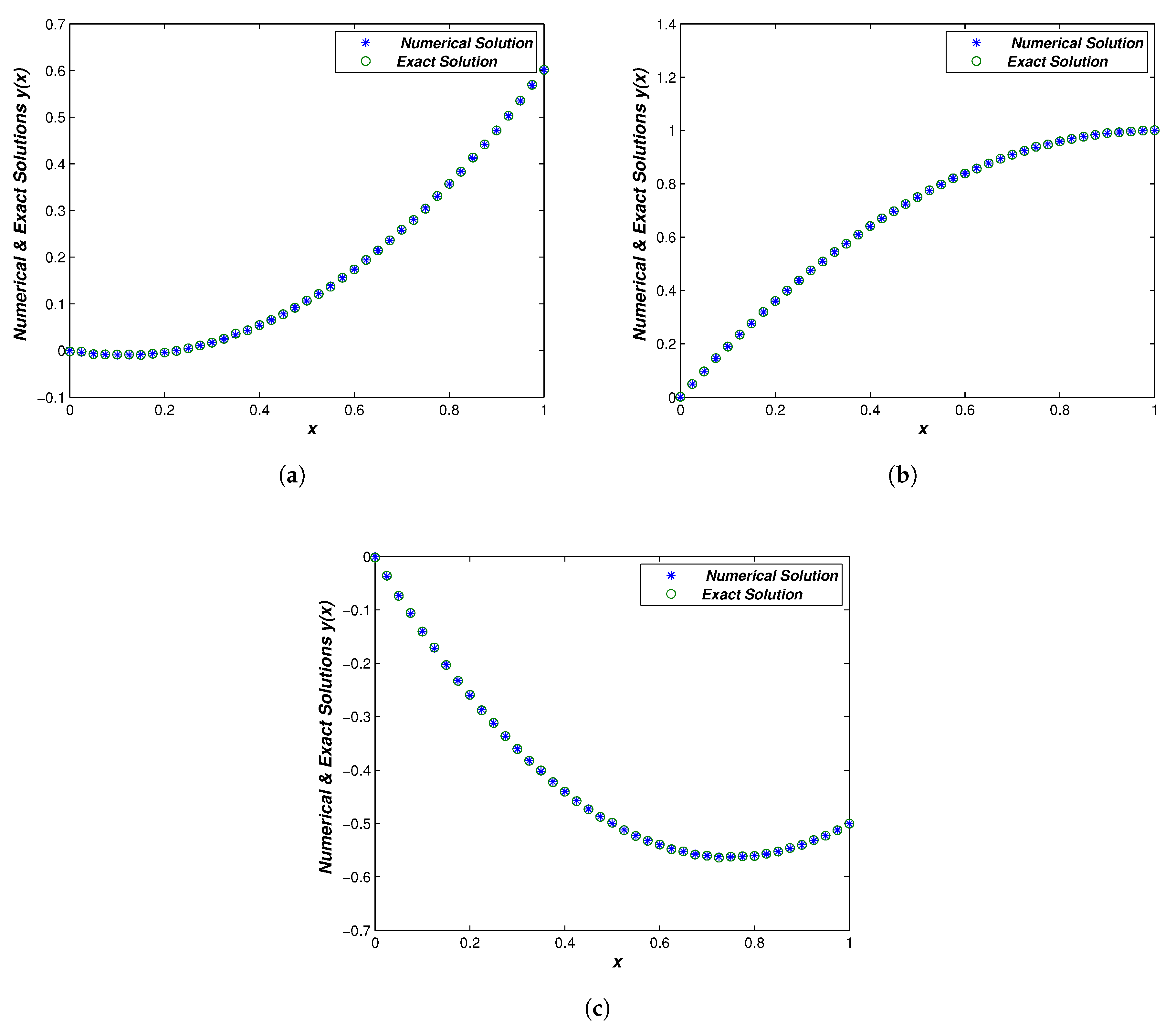
5. Implementations (Numerical Examples)

In this section, we introduce two types of dynamical problems. The numerical method introduced in Section 4 has been used for solving the optimal control problems of integer and fractional order with free and non-free terminal time.

Example 1.

Let us take into consideration the following (FOC) problem with non-free terminal time introduced by [10,25].

$$\begin{array}{c}\hfill \underset{x\left(\tau \right),u\left(\tau \right)}{min}J(\tau ,x\left(\tau \right),u\left(\tau \right))=\underset{x\left(\tau \right),u\left(\tau \right)}{min}{\int }_0^1{(\tau u\left(\tau \right)-(\gamma +2)x\left(\tau \right))}^{2}d\tau ,\end{array}$$

(15)

subjected to the dynamic system

$$\begin{array}{c}\hfill D^{\gamma }x\left(\tau \right)+\dot{x}\left(\tau \right)={\tau }^2+u\left(\tau \right),\end{array}$$

(16)

with the boundary conditions (BCs)

$$\begin{array}{c}\hfill x\left(0\right)=0,x\left(1\right)=\frac{2}{3+\gamma },\end{array}$$

(17)

where the exact solution is given by

$$(x\left(\tau \right),u\left(\tau \right))=(\frac{2{\tau }^{2+\gamma }}{\mathsf{\Gamma }(3+\gamma )},\frac{2{\tau }^{1+\gamma }}{\mathsf{\Gamma }(2+\gamma )}).$$

Using the approximation base $\mathsf{\Omega }\left(t\right)=\{{\tau }^2,\tau ,1\}$, we have the approximation of $x\left(\tau \right)$ as

$$\begin{array}{c}\hfill x\left(\tau \right)=c_0+c_1\tau +c_2{\tau }^2.\end{array}$$

(18)

If we use the BCs in Equation (17), we obtain $c_0=0$ and $c_1=\frac{2}{3+\gamma }-c_2$. Then, the following approximation is obtained

$$\begin{array}{c}\hfill x\left(t\right)=t(c_2+\frac{2}{3+\gamma }-c_{2}t).\end{array}$$

(19)

Then, we have

$$\begin{array}{c}\hfill u\left(\tau \right)=x\left(\tau \right)=(1+{\tau }^{1-\gamma })(c_2-\frac{2}{3+\gamma }+2c_2\tau )-{\tau }^2.\end{array}$$

(20)

Substitute Equations (19) and (20) in the problem of minimizing in the Equation (15) to obtain the optimal values of $c_2,$ and the non-free terminal parameter $T.$ Hence, using the Hooke and Jeeves method for the problem in parameter $c_2$, the approximation of the problem is plotted in Figure 1a.

Example 2.

Consider the following integer-order optimal control problem with non-free terminal time:

$$\begin{array}{c}\hfill \underset{x\left(\tau \right),u\left(\tau \right),T}{min}J(\tau ,x\left(\tau \right),u\left(\tau \right),T)=\underset{x\left(\tau \right),u\left(\tau \right),T}{min}{\int }_0^T{(\tau u\left(\tau \right)-2x\left(\tau \right))}^{2}d\tau ,\end{array}$$

(21)

subjected to the dynamic system

$$\begin{array}{c}\hfill \dot{\dot{x}}\left(\tau \right)+\dot{x}\left(\tau \right)={\tau }^2+u\left(\tau \right),\end{array}$$

(22)

with the boundary conditions

$$\begin{array}{c}\hfill x\left(0\right)=0,x\left(1\right)=1,\end{array}$$

(23)

where the exact solution is given by

$$(x\left(\tau \right),u\left(\tau \right))=(\tau (2-\tau ),-{\tau }^2+2\tau +2).$$

Consider the solution of the optimization problem in Equations (21)–(23) written as follows

$$\begin{array}{c}\hfill x\left(\tau \right)=\tau (1+c_2-c_2\tau ).\end{array}$$

(24)

This satisfies the boundary conditions in Equation (23). Then, we have

$$\begin{array}{c}\hfill u\left(\tau \right)=-{\tau }^2+2c_{2}t+3c_2-1.\end{array}$$

(25)

Substitute Equations (24) and (25) in minimizing the problem in Equation (21) to obtain the optimal values of $c_2=0.989$ and $T=0.997$. Hence, the approximation of the problem is written as $x\left(\tau \right)=\tau (2-\tau )$ and then, it is plotted in Figure 1b.

Example 3.

Let us consider the following optimal control problem of fractional order with non-free terminal time which was introduced by [25]

$$\begin{array}{c}\hfill \underset{x\left(\tau \right),u\left(\tau \right),T}{min}J(\tau ,x\left(\tau \right),u\left(\tau \right),T)=\underset{x\left(\tau \right),u\left(\tau \right),T}{min}{\int }_0^T{(\tau u\left(\tau \right)-(\gamma +2)x\left(\tau \right))}^{2}d\tau ,\end{array}$$

(26)

subject to the control system

$$\begin{array}{c}\hfill D_{\tau }^{\gamma }x\left(\tau \right)+\dot{x}\left(\tau \right)={\tau }^2+u\left(\tau \right),\end{array}$$

(27)

and the boundary conditions

$$\begin{array}{c}\hfill x\left(0\right)=0,x\left(T\right)=1.\end{array}$$

(28)

Consider the solution of the optimization problem in Equations (26)–(28) written as follows:

$$\begin{array}{c}\hfill x\left(\tau \right)=c_2{\tau }^2+(\frac{1}{T}-c_{2}T)\tau ,\end{array}$$

(29)

which satisfied the boundary conditions in Equation (28). Then, we have

$$\begin{array}{c}\hfill u\left(\tau \right)=-{\tau }^2+2c_2\tau +3c_2-1.\end{array}$$

(30)

Substitute Equations (29) and (30) in minimizing the problem in Equation (26) to obtain the optimal solutions using the Hooke and Jeeves method. Hence, the approximation of the problem is plotted in Figure 1c.

6. Discussion and Conclusions

The main purpose of this study is to introduce numerical methods for solving two cases of fractional-order optimal dynamical control systems with free and non-free terminal time. The study also offers a comparison of the numerical results obtained by using the proposed method with the exact solutions for three test problems. From the numerical results of the proposed method, we observe that the method is applicable to a class of (FOC) problems with free or non-free terminal time. Moreover, the proposed method achieves good agreement with exact solutions. As a result, the new method is efficient and provides encouraging results. This direction of this research can be extended in the future to new directions such as improving the numerical studies of stochastic optimal control problems to the continuity of the research in this domain.

References

1. Longuski, J.M.; Guzmán, J.J.; Prussing, J.E. Optimal Control with Aerospace Applications; Springer: Cham, Switzerland, 2014. [Google Scholar]
2. Agrawal, O.P. A formulation and numerical scheme for fractional optimal control problems. J. Vib. Control. 2008, 14, 1291–1299. [Google Scholar] [CrossRef]
3. Sweilam, N.; Hassan, A.-A.; Tamer, M.; Hoppe, R.H.W. Numerical solution of some types of fractional optimal control problems. Sci. World J. 2013, 2013, 306237. [Google Scholar] [CrossRef] [PubMed] [Green Version]
4. Bhrawy, A.H.; Doha, E.H.; Baleanu, D.; Ezz-Eldien, S.S.; Abdelkawy, M.A. An accurate numerical technique for solving fractional optimal control problems. Differ. Equ. 2015, 15, 23. [Google Scholar]
5. Akbarian, T.; Keyanpour, M. A new approach to the numerical solution of fractional order optimal control problems. Appl. Appl. Math. 2013, 8, 523–534. [Google Scholar]
6. Bhrawy, A.H.; Doha, E.H.; Tenreiro Machado, J.A.; Ezz-Eldien, S.S. An efficient numerical scheme for solving multi-dimensional fractional optimal control problems with a quadratic performance index. Asian J. Control 2015, 17, 2389–2402. [Google Scholar] [CrossRef] [Green Version]
7. Doha, E.H.; Bhrawy, A.H.; Ezz-Eldien, S.S. An efficient Legendre spectral tau matrix formulation for solving fractional subdiffusion and reaction subdiffusion equations. J. Comput. Nonlinear Dyn. 2015, 10, 021019. [Google Scholar] [CrossRef]
8. Liu, J.; Hou, G. Numerical solutions of the space-and time-fractional coupled Burgers equations by generalized differential transform method. Appl. Math. Comput. 2011, 217, 7001–7008. [Google Scholar] [CrossRef]
9. Lotfi, A.; Dehghan, M.; Yousefi, S.A. A numerical technique for solving fractional optimal control problems. Comput. Math. Appl. 2011, 62, 1055–1067. [Google Scholar] [CrossRef] [Green Version]
10. Pooseh, S.; Almeida, R.; Torres, D.F.M. A numerical scheme to solve fractional optimal control problems. Conf. Pap. Sci. 2013, 2013, 165298. [Google Scholar] [CrossRef] [Green Version]
11. Zhao, Z.; Li, C. Fractional difference/finite element approximations for the time–space fractional telegraph equation. Appl. Math. Comput. 2012, 219, 2975–2988. [Google Scholar] [CrossRef]
12. Mechee, M.S.; Senu, N. Numerical Study of Fractional Differential Equations of Lane-Emden Type by Method of Collocation; Scientific Research Publishing: Wuhan, China, 2012. [Google Scholar]
13. Zhou, H.; Tian, W.Y.; Deng, W. Quasi-compact finite difference schemes for space fractional diffusion equations. J. Sci. Comput. 2013, 56, 45–66. [Google Scholar] [CrossRef] [Green Version]
14. Bhrawy, A.H.; Doha, E.H.; Ezz-Eldien, S.S.; Van Gorder, R.A. A new Jacobi spectral collocation method for solving 1 + 1 fractional Schrödinger equations and fractional coupled Schrödinger systems. Eur. Phys. J. Plus 2014, 129, 1–21. [Google Scholar] [CrossRef]
15. Bhrawy, A.H.; Ezz-Eldien, S.S.; Doha, E.H.; Abdelkawy, M.A.; Baleanu, D. Solving fractional optimal control problems within a Chebyshev–Legendre operational technique. Int. J. Control 2017, 90, 1230–1244. [Google Scholar] [CrossRef]
16. Yousefi, S.A.; Lotfi, A.; Dehghan, M. The use of a Legendre multiwavelet collocation method for solving the fractional optimal control problems. J. Vib. Control. 2011, 17, 2059–2065. [Google Scholar] [CrossRef]
17. Bhrawy, A.H.; Ezz-Eldien, S.S. A new Legendre operational technique for delay fractional optimal control problems. Calcolo 2016, 53, 521–543. [Google Scholar] [CrossRef]
18. Heydari, M.H.; Hooshmandasl, M.R.; Mohammadi, F. Legendre wavelets method for solving fractional partial differential equations with Dirichlet boundary conditions. Appl. Math. Comput. 2014, 234, 267–276. [Google Scholar] [CrossRef]
19. Khan, R.A.; Khalil, H. A new method based on legendre polynomials for solution of system of fractional order partial differential equations. Int. J. Comput. Math. 2014, 91, 2554–2567. [Google Scholar] [CrossRef]
20. Sweilam, N.H.; Al-Ajami, T.M. Legendre spectral-collocation method for solving some types of fractional optimal control problems. J. Adv. Res. 2015, 6, 393–403. [Google Scholar] [CrossRef] [Green Version]
21. Sweilam, N.H.; Nagy, A.M.; El-Sayed, A.A. Second kind shifted Chebyshev polynomials for solving space fractional order diffusion equation. Chaos Solitons Fractals 2015, 73, 141–147. [Google Scholar] [CrossRef]
22. Almeida, R.; Torres, D.F.M. A discrete method to solve fractional optimal control problems. Nonlinear Dyn. 2015, 80, 1811–1816. [Google Scholar] [CrossRef] [Green Version]
23. Suárez, J.I.; Vinagre, B.M.; Chen, Y. A fractional adaptation scheme for lateral control of an AGV. J. Vib. Control 2008, 14, 1499–1511. [Google Scholar] [CrossRef]
24. Pinto, C.; Tenreiro Machado, J.A. Fractional dynamics of computer virus propagation. Math. Probl. Eng. 2014, 2014, 476502. [Google Scholar] [CrossRef] [Green Version]
25. Pooseh, S.; Almeida, R.; Torres, D.F.M. Fractional order optimal control problems with free terminal time. arXiv 2013, arXiv:1302.1717. [Google Scholar] [CrossRef] [Green Version]
26. Jafari, H.; Tajadodi, H. Fractional order optimal control problems via the operational matrices of Bernstein polynomials. UPB Sci. Bull. 2014, 76, 115–128. [Google Scholar]
27. Jesus, I.S.; Tenreiro, M.J.A. Fractional control of heat diffusion systems. Nonlinear Dyn. 2008, 54, 263–282. [Google Scholar] [CrossRef] [Green Version]
28. Ahmad, W.M.; El-Khazali, R. Fractional-order dynamical models of love. Chaos Solitons Fractals 2007, 33, 1367–1375. [Google Scholar] [CrossRef]
29. David, S.A.; Linares, J.L.; Pallone, E.M.J.A. Fractional order calculus: Historical apologia, basic concepts and some applications. Rev. Bras. Ensino Física 2011, 33, 4302. [Google Scholar] [CrossRef]
30. Bohannan, G.W. Analog fractional order controller in temperature and motor control applications. J. Vib. Control. 2008, 14, 1487–1498. [Google Scholar] [CrossRef]
31. Joshi, H.J.; Brajesh, K. 2D dynamic analysis of the disturbances in the calcium neuronal model and its implications in neurodegenerative disease. Cogn. Neurodynam. 2022, 1–12. [Google Scholar] [CrossRef]
32. Zhang, S.; Zhang, H.-Q. Fractional sub-equation method and its applications to nonlinear fractional PDEs. Phys. Lett. A 2011, 375, 1069–1073. [Google Scholar] [CrossRef]
33. Kreyszig, E. Introductory Functional Analysis with Applications; John Wiley & Sons: Hoboken, NJ, USA, 1991; Volume 17. [Google Scholar]
34. Zhao, Y.; Li, Y.; Liu, H. Fractional-order Iterative Learning Control with Nonuniform Trial Lengths. Int. J. Control. Autom. Syst. 2022, 20, 3167–3176. [Google Scholar] [CrossRef]
35. Matt, C.; Hess, T.; Benlian, A. Digital transformation strategies. Bus. Inf. Syst. Eng. 2015, 57, 339–343. [Google Scholar] [CrossRef]
36. Zhao, Y.; Li, Y.; Zhang, F.; Liu, H. Iterative learning control of fractional-order linear systems with nonuniform pass lengths. Trans. Inst. Meas. Control. 2022, 44, 3071–3080. [Google Scholar] [CrossRef]
37. Sabermahani, S.; Ordokhani, Y. Fibonacci wavelets and Galerkin method to investigate fractional optimal control problems with bibliometric analysis. J. Vib. Control. 2021, 27, 1778–1792. [Google Scholar] [CrossRef]
Figure 1. A Comparison of Numerical Solutions of (FrOCDS) Evaluated by the Hooke and Jeeves Direct Search Method for the Implementations in (a) Example 1, (b) Example 2, and (c) Example 3.
Symmetry 15 00624 g001
Disclaimer/Publisher’s Note: The statements, opinions and data contained in all publications are solely those of the individual author(s) and contributor(s) and not of MDPI and/or the editor(s). MDPI and/or the editor(s) disclaim responsibility for any injury to people or property resulting from any ideas, methods, instructions or products referred to in the content.