A Tau Approach for Solving Time-Fractional Heat Equation Based on the Shifted Sixth-Kind Chebyshev Polynomials

Abstract

The time-fractional heat equation governed by nonlocal conditions is solved using a novel method developed in this study, which is based on the spectral tau method. There are two sets of basis functions used. The first set is the set of non-symmetric polynomials, namely, the shifted Chebyshev polynomials of the sixth-kind (CPs6), and the second set is a set of modified shifted CPs6. The approximation of the solution is written as a product of the two chosen basis function sets. For this method, the key concept is to transform the problem governed by the underlying conditions into a set of linear algebraic equations that can be solved by means of an appropriate numerical scheme. The error analysis of the proposed extension is also thoroughly investigated. Finally, a number of examples are shown to illustrate the reliability and accuracy of the suggested tau method.

1. Introduction

The exploration of orthogonal polynomials has expanded in recent years, a topic that is related to several important branches of analysis. Various differential and integral equations can be solved using them. Additionally, it has been shown that orthogonal polynomials have applications in quantum mechanics and mathematical statistics. Numerous papers have sought to explore these polynomials and their applications because of their significance. One may consult [1,2,3].

The different special polynomials can be classified into symmetric and non-symmetric ones. Among the important orthogonal polynomials are the Chebyshev polynomials, which are highly regarded for their significance. The four well-known Chebyshev polynomials are all special cases of Jacobi polynomials [4]. The first and second-kinds are symmetric polynomials, while the third- and fourth- kinds are non-symmetric ones. All of the kinds of Chebyshev polynomials are extremely important in fields such as numerical analysis and approximation theory. Several studies, both historical and modern, focus on deriving numerical solutions of different differential equations using Chebyshev polynomials of the first kind, for instance, see [5,6,7,8,9]. In addition, Chebyshev polynomials of the second-, third-, and fourth-kinds were also put to use in a wide range of contexts; for example, see [10,11,12,13,14,15]. Two new families of symmetric Chebyshev polynomials have been introduced recently; they are called the fifth- and sixth-kinds of Chebyshev polynomials, respectively. In fact, these polynomials can be viewed as special cases of the symmetric generalized ultraspherical polynomials, see [16]. Furthermore, in [17], Masjed–Jamei found two half-trigonometric representations for the fifth- and sixth-kinds, whereas Abd-Elhameed and Youssri in [18,19] found complete trigonometric representations for these kinds of Chebyshev polynomials. May contributions regarding, fifth- and sixth- kinds of Chebyshev polynomials were performed, see, for example [20,21,22,23].

The study of derivatives and the integration of arbitrary orders is central to fractional calculus, a field that was initially viewed as purely theoretical. In the last decades, it has been shown that fractional calculus can be used to explain many phenomena as diverse as fluid flow, aerodynamics, electrochemistry of corrosion, biology, optics, finance, and signal processing, and it has recently attracted the attention of a large number of researchers [24,25,26,27]. The development of exact solutions to a variety of fractional differential equations (FDEs) is not available, so it is an important challenge to investigate the different types of FDEs using various effective numerical techniques. Some methods have been introduced to the FDEs such as the Fourier transform method [28], the finite element method [29], the iterative method in [30], and the Jacobi spectral method in [31]. The vast majority of nonlinear FDEs cannot be solved exactly analytically, so numerical techniques may be employed; see, for example [32,33,34].

Fractional partial differential equations (FPDEs) have recently attracted the attention of a rising number of authors due to their utility in many areas of science and other disciplines (see, for example, [35,36]). This is due to the more accurate and complete representation of a wider range of phenomena provided by mathematical models constructed on derivatives of factorial order, either in time or space or both. There are many different approaches to treat the models described by FPDEs that are employed in the applied sciences. The KDV-type FDEs are among the most important PFDES. Some authors have shown an interest in tackling these types of equations. To treat the space-time-fractional KdV equation, for instance, the authors of [37] used the variational iteration method. The linearized time-fractional KDV-type equations are solved using the spectral tau method in [38]. Furthermore, the authors of [39] addressed the time-fractional Black–Scholes equation. Hybrid functions were used in [36] to solve a PFDES problem in two dimensions. Other contributions regarding the different spectral methods can be found in [40,41,42].

Spectral methods are the most common methods used in obtaining the numerical solution of differential equations. The main feature of these methods is that they assume approximate solutions to various types of differential equations as combinations of orthogonal polynomials, specifically orthogonal polynomials. The three methods, namely, collocation, Galerkin, and tau, are the different spectral methods used to obtain the desired numerical solutions. Regarding the collocation method, it is the most commonly used method due to its simplicity and applicability to all types of differential equations. For instance, Atta et al. [43] utilized a collocation procedure for solving multi-term fractional differential equations. In addition, the authors in [44] followed a collocation approach to solve a certain non-linear time-fractional partial integro-differential. Regarding the tau method, it is also utilized for solving various differential equations. Abd-Elhameed et al. [45] handled the non-linear Fisher Equation. Youssri in [46] used the tau method to solve the fractional Bagley–Torvik equation. The authors in [47] employed an operational tau method for handling a class of fractional integro-differential equations. Regarding the Galerkin method, it can be applied effectively to linear equations. For example, Doha et al. [48] employed the Galerkin method for treating the linear, one-dimensional telegraph-type equation.

The main purpose of our manuscript is to treat numerically the time-fractional differential equation using the shifted sixth-kind Chebyshev polynomials. The main outlines of our contribution in this paper can be listed in the following issues:

• Some specific integer and fractional derivatives of the shifted sixth-kind Chebyshev polynomials and their modified ones are expressed in terms of their original ones.
• The tau approach is applied to treat the time-fractional differential equations.
• The matrix system resulting from the application of the tau method is treated via a suitable numerical solver.
• The convergence of the double Chebyshev expansion is examined.
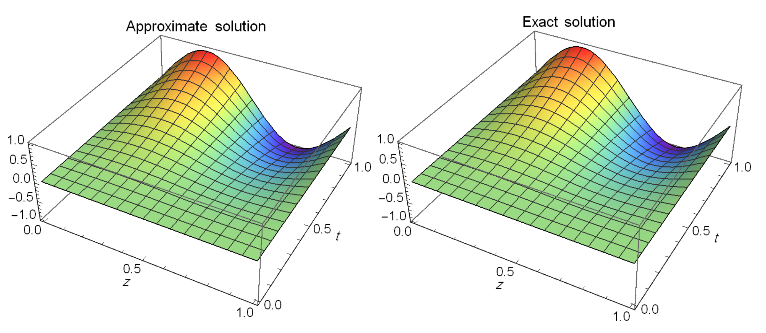
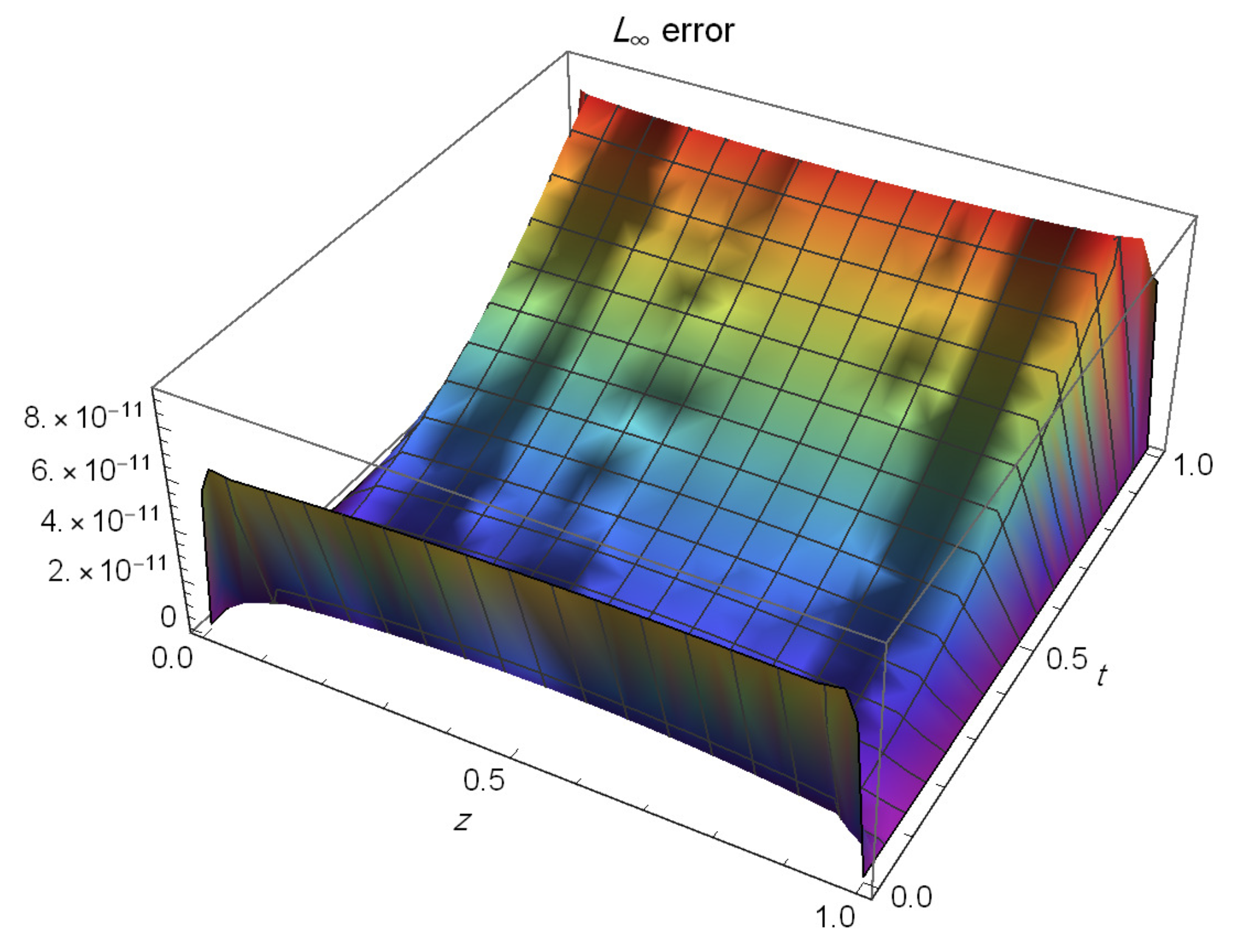
• Numerical examples are given, along with several comparisons with some other related papers, to demonstrate the applicability and efficiency of our proposed tau approach.

An outline of this paper is as follows: in Section 2, we present some preliminary and essential relations of fractional calculus, and the shifted Chebyshev polynomials of the sixth kind. In Section 3, we introduce the tau approach for the treatment of the time-fractional heat equation. Section 4 delves into the convergence and error analysis. In Section 5, we introduce some examples to illustrate the efficiency and accuracy of the method that we used. Finally, the conclusion is presented in Section 6.

2. Some Fundamentals and Useful Formulas

In this section, we will look at the basics of fractional calculus, including some definitions and properties. Moreover, several essential characteristics of the CPs6 and their shifted ones will be accounted for.

2.1. An Account for the Fractional Calculus

Definition 1

([49]). On the standard Lebesgue space $L_1[0,1]$, the Riemann-Liouville fractional integral operator $I^{\rho }$of order ρ is defined as

$$I^{\rho }h\left(x\right)=\left\{\begin{array}{cc}{\displaystyle \frac{1}{\mathsf{\Gamma }\left(\rho \right)}{\int }_0^x{(x-z)}^{\rho -1}h\left(z\right)dz,}\hfill & \rho >0,\hfill \\ h\left(x\right),\hfill & \rho =0.\hfill \end{array}\right.$$

Definition 2

([49]). Derivatives of fractional orders, as defined by Caputo, are as follows:

$${\displaystyle D^{\rho }h\left(x\right)=\frac{1}{\mathsf{\Gamma }(m-\rho )}{\int }_0^x{(x-z)}^{m-\rho -1}{h}^{\left(m\right)}\left(z\right)dz,\rho >0,x>0,}$$

where $m-1⩽\rho <m,m\in \mathbb{N}$.

The following properties are satisfied: for $m-1⩽\rho <m,m\in \mathbb{N},$

$$\begin{array}{cc}\hfill & \left(i\right)\left(D^{\rho }{I}^{\rho }h\right)\left(y\right)=h\left(y\right),\hfill \\ \hfill & \left(ii\right)\left(I^{\rho }{D}^{\rho }h\right)\left(y\right)=h\left(y\right)-\sum _{k=0}^{m-1}\frac{h^{\left(k\right)}\left(0^{+}\right)}{\mathsf{\Gamma }(k+1)}{(y-a)}^k,y>0,\hfill \\ \hfill & \left(iii\right)D^{\rho }{y}^{\delta }=\frac{\mathsf{\Gamma }(\delta +1)}{\mathsf{\Gamma }(\delta +1-\rho )}{y}^{\delta -\rho },\delta \in \mathbb{N},\delta \ge \lceil \rho \rceil ,\hfill \end{array}$$

where $\lceil \rho \rceil$ is the lowest positive integer that is greater than or equal to $\rho$.

2.2. Some Properties and Relations of the CPs6

In this section, we will discuss the CPs6 and their shifted ones, highlighting some of their features.

The CPs6 $Y_m\left(t\right)$ are orthogonal polynomials on $[-1,1]$ in the sense that

$${\int }_{-1}^1{t}^2\sqrt{1-t^2}{Y}_m\left(t\right)Y_{\ell }\left(t\right)dt=\left\{\begin{array}{cc}{h}_{\ell },\hfill & if m=\ell ,\hfill \\ 0,\hfill & if m\ne \ell ,\hfill \end{array}\right.$$

and

$${\displaystyle h_{\ell }=\frac{\pi }{2^{2\ell +3}}\left\{\begin{array}{cc}1,\hfill & \ell \mathrm{even},\hfill \\ {\displaystyle \frac{\ell +3}{\ell +1},}\hfill & \ell \mathrm{odd}.\hfill \end{array}\right.}$$

The following three-term recurrence relation can be used to generate the polynomials $Y_i\left(t\right)$:

$$Y_{\ell }\left(t\right)=t{Y}_{\ell -1}\left(t\right)-{\alpha }_{\ell }{Y}_{\ell -2}\left(t\right),Y_0\left(t\right)=1,Y_1\left(t\right)=t,\ell \ge 2,$$

with

$${\alpha }_{\ell }=\frac{\ell (\ell +1)+{(-1)}^{\ell }(2\ell +1)+1}{4\ell (\ell +1)}.$$

The authors in [18] proved the following trigonometric representation for the CPs6:

$$Y_{\ell }\left(cos\varphi \right)=\left\{\begin{array}{cc}{\displaystyle \frac{sin\left((\ell +2)\varphi \right)}{2^{\ell }sin\left(2\varphi \right)},}\hfill & \ell \mathrm{even},\hfill \\ {\displaystyle \frac{sin\left((\ell +1)\varphi \right)+(\ell +1)cos\left(\varphi \right)sin\left((\ell +2)\varphi \right)}{2^{\ell +1}(\ell +1){cos}^2\left(\varphi \right)sin\left(\varphi \right)},}\hfill & \ell \mathrm{odd}.\hfill \end{array}\right.$$

he shifted CPs6 on $[0,\tau ],\tau >0$ can be defined as [18]:

$$Y_{\ell }^{*}\left(t\right)=Y_{\ell }\left(\frac{2t}{\tau }-1\right).$$

The recursive formula

$$Y_{\ell }^{*}\left(t\right)=\left(\frac{2t}{\tau }-1\right)Y_{\ell -1}^{*}\left(t\right)-{\alpha }_{\ell }{Y}_{\ell -2}^{*}\left(t\right),Y_0^{*}\left(t\right)=1,Y_1^{*}\left(t\right)=\frac{2t}{\tau }-1,\ell \ge 2,$$

constructs ${\left\{Y_{\ell }^{*}\left(t\right)\right\}}_{\ell \ge 0}$. These polynomials have the next orthogonality relation:

$${\int }_0^{\tau }w\left(t\right)Y_m^{*}\left(t\right)Y_{\ell }^{*}\left(t\right)dt=h_{\tau ,m}{\delta }_{m,\ell },$$

(1)

where $w\left(t\right)={(2t-\tau )}^2\sqrt{t\tau -t^2},$

$${\delta }_{m,\ell }=\left\{\begin{array}{cc}1,\hfill & \mathrm{if}m=\ell ,\hfill \\ 0,\hfill & \mathrm{if}m\ne \ell ,\hfill \end{array}\right.$$

and

$$h_{\tau ,\ell }=\frac{\pi {\tau }^4}{2^{2\ell +5}}\left\{\begin{array}{cc}1,\hfill & \mathrm{if}\ell \mathrm{even},\hfill \\ \frac{\ell +3}{\ell +1},\hfill & \mathrm{if}\ell \mathrm{odd}.\hfill \end{array}\right.$$

(2)

The analytic formula of $Y_j^{*}\left(t\right)$ is [18]

$$Y_j^{*}\left(t\right)=\sum _{r=0}^j{B}_{r,j}{t}^r,$$

(3)

where

$${\displaystyle B_{r,j}=\frac{2^{2r-j}}{{\tau }^r(2r+1)!}\left\{\begin{array}{cc}{\displaystyle \sum _{\ell =\lfloor \frac{r+1}{2}\rfloor }^{\lfloor \frac{j}{2}\rfloor }\frac{{(-1)}^{\frac{j}{2}+\ell +r}(2\ell +r+1)!}{(2\ell -r)!},}\hfill & \mathrm{if} j\mathrm{even},\hfill \\ {\displaystyle \frac{2}{j+1}\sum _{\ell =\lfloor \frac{r}{2}\rfloor }^{\lfloor \frac{j-1}{2}\rfloor }\frac{{(-1)}^{\frac{j+1}{2}+\ell +r}(\ell +1)(2\ell +r+2)!}{(2\ell -r+1)!},}\hfill & \mathrm{if}j\mathrm{odd}.\hfill \end{array}\right.}$$

The inversion formula of $Y_j^{*}\left(t\right)$ is [18]

$$t^{\ell }=\sum _{m=0}^{\ell }{Q}_{m,\ell }{Y}_m^{*}\left(t\right),$$

where

$$Q_{m,\ell }=\frac{{\tau }^{\ell }(2\ell +1)!2^{m-2\ell +2}}{(\ell -m)!(m+\ell +4)!}\left\{\begin{array}{cc}(m+2)\left(m(m+4)+{\ell }^2+\ell +3\right),\hfill & \mathrm{if}m\mathrm{even},\hfill \\ (m+1)\left(m\right(m+4)+\ell (\ell +3)+6),\hfill & \mathrm{if}m\mathrm{odd}.\hfill \end{array}\right.$$

3. Treatment of the Time-Fractional Heat Equation

Here, we will focus on the implementation of a numerical algorithm that employs the tau method to solve the time-fractional heat equation. The method relies on employing two orthogonal polynomials in terms of the CPs6, which are used as the basis functions. For the development of our suggested numerical algorithm, we will also derive two formulas for the derivatives of the basis functions.

3.1. Basis Functions and Their Derivatives

In this section, we select two sets of basis functions. The first set is a certain set of modified CPs6, and the second set is the CPs6 set.

Now, consider the following basis functions:

$$\begin{array}{cc}\hfill {\psi }_i\left(z\right)=& z(l-z)Y_i^{*}\left(z\right),\hfill \end{array}$$

along with $Y_j^{*}\left(t\right)$ defined in Equation (3).

We may write the orthogonality relation of ${\psi }_i\left(z\right)$ as:

$${\int }_0^l\overline{w}\left(z\right){\psi }_i\left(z\right){\psi }_j\left(z\right)dx=h_{l,i}{\delta }_{i,j},$$

(4)

where $\overline{w}\left(z\right)=\frac{{(2z-l)}^2}{z^{\frac{3}{2}}{(l-z)}^{\frac{3}{2}}}$ and $h_{\tau ,i}$ is as given in (2).

In the following theorem, we show how to represent the second-order derivative of modified CPs6 in terms of the original Chebyshev polynomials.

Theorem 1.

The explicit expression for the second-order derivative of ${\psi }_m\left(z\right)$ is [44]:

$${\displaystyle \frac{d^2{\psi }_m\left(z\right)}{d{z}^2}=\sum _{\ell =0}^m{\lambda }_{\ell ,m}{Y}_{\ell }^{*}\left(z\right),}$$

where

$${\lambda }_{\ell ,m}=\frac{1}{2^{m-\ell -1}}\left\{\begin{array}{cc}\frac{-(m+1)(m+2)}{2},\hfill & ifm=\ell ,\hfill \\ \ell +2,\hfill & ifm,\ell \mathit{even}and\frac{m-\ell +2}{2}\mathit{odd},\hfill \\ -3(\ell +2),\hfill & ifm,\ell \mathit{even}and\frac{m-\ell +2}{2}\mathit{even},\hfill \\ \frac{-(\ell +1)(m+2\ell +6)}{m+1},\hfill & ifm,\ell \mathit{odd}and\frac{m-\ell +2}{2}\mathit{even},\hfill \\ \frac{(\ell +1)(-m+2\ell +2)}{m+1},\hfill & ifm,\ell \mathit{odd}and\frac{m-\ell +2}{2}\mathit{odd},\hfill \\ 0,\hfill & \mathit{otherwise}.\hfill \end{array}\right.$$

The fractional derivative of the shifted CPS6 may be approximated as in the following theorem.

Theorem 2.

The following is an approximation for $D_t^{\alpha }{Y}_j^{*}\left(t\right)$, $0<\alpha <1$

$$D_t^{\alpha }{Y}_j^{*}\left(t\right)\approx \sum _{k=0}^N{\sigma }_{k,j,\alpha }{Y}_k^{*}\left(t\right),$$

where

$${\sigma }_{k,j,\alpha }=\sum _{r=1}^j\frac{\left(r\right)!B_{r,j}{\rho }_{k,r,\alpha }}{\mathsf{\Gamma }(r-\alpha +1)}.$$

Proof. 

Applying $D^{\alpha }$ to Equation (3) results in

$$D^{\alpha }{Y}_j^{*}\left(t\right)=\sum _{r=1}^j{B}_{r,j}\frac{\left(r\right)!}{\mathsf{\Gamma }(r-\alpha +1)}{t}^{r-\alpha }.$$

(5)

Now, assume that $t^{r-\alpha }$ can be approximated as

$$t^{r-\alpha }\approx \sum _{k=0}^N{\rho }_{k,r,\alpha }{Y}_k^{*}\left(t\right).$$

(6)

To compute ${\rho }_{k,r,\alpha }$, we use the orthogonality relation of $Y_k^{*}\left(t\right)$ in (1) to obtain

$$\begin{array}{cc}\hfill {\rho }_{k,r,\alpha }& =\frac{1}{h_{\tau ,k}}{\int }_0^{\tau }{t}^{r-\alpha }{Y}_k^{*}\left(t\right)\omega \left(t\right)dt\hfill \\ & =\frac{1}{h_{\tau ,k}}\sum _{\ell =0}^k{B}_{\ell ,k}{\int }_0^{\tau }{t}^{r+\ell -\alpha +1}{(2t-\tau )}^2\sqrt{t\tau -t^2}\hfill \\ & =\frac{1}{h_{\tau ,k}}\sum _{\ell =0}^k{B}_{\ell ,k}{\int }_0^{\tau }\left(4t^{r+\ell -\alpha +\frac{5}{2}}+{\tau }^2{t}^{r+\ell -\alpha +\frac{1}{2}}-4\tau t^{r+\ell -\alpha +\frac{3}{2}}\right)\sqrt{\tau -t}dt\hfill \\ & =\frac{1}{h_{\tau ,k}}\sum _{\ell =0}^k{B}_{\ell ,k}{\tau }^{r+\ell -\alpha +4}\left\{4\beta \left(r+\ell -\alpha +\frac{7}{2},\frac{3}{2}\right)+\beta \left(r+\ell -\alpha +\frac{3}{2},\frac{3}{2}\right)\right.\hfill \\ \hfill & \left.-4\beta \left(r+\ell -\alpha +\frac{5}{2},\frac{3}{2}\right)\right\}\hfill \\ & =\frac{1}{h_{\tau ,k}}\sum _{\ell =0}^k{B}_{\ell ,k}{\tau }^{r+\ell -\alpha +4}\mathsf{\Gamma }\left(\frac{3}{2}\right)\left(\frac{4\mathsf{\Gamma }(r+\ell -\alpha +\frac{7}{2})}{\mathsf{\Gamma }(r+\ell -\alpha +5)}+\frac{\mathsf{\Gamma }(r+\ell -\alpha +\frac{3}{2})}{\mathsf{\Gamma }(r+\ell -\alpha +3)}\right.\hfill \\ \hfill & \left.-\frac{4\mathsf{\Gamma }(r+\ell -\alpha +\frac{5}{2})}{\mathsf{\Gamma }(r+\ell -\alpha +4)}\right),\hfill \end{array}$$

$$\begin{array}{cc}\hfill {\rho }_{k,r,\alpha }=& \frac{1}{h_{\tau ,k}}\sum _{\ell =0}^k{B}_{\ell ,k}{\tau }^{r+\ell -\alpha +4}\frac{\sqrt{\pi }(3+\ell +{\ell }^2+r+2\ell r+r^2-\alpha -2(\ell +r)\alpha +{\alpha }^2)}{2\mathsf{\Gamma }(5+\ell +r+\alpha )}\hfill \\ \hfill & \times \mathsf{\Gamma }\left(\frac{3}{2}+\ell +r-\alpha \right),\hfill \end{array}$$

where $\beta (.,.)$ and $\mathsf{\Gamma }(.)$ are the familiar Beta and Gamma functions.

By substituting Equation (6) into Equation (5), we obtain the desired result. □

3.2. Tau Solution for Time-Fractional Heat Equation

This section describes in detail the algorithm that will be employed for treating the time-fractional heat equation.

Consider the following time-fractional heat equation [50,51]:

$$\frac{{\partial }^{\gamma }u(z,t)}{\partial t^{\gamma }}=\frac{{\partial }^{2}u(z,t)}{\partial z^2}+q(z,t),0<\gamma \le 1,$$

(7)

governed by the nonlocal conditions

$$u(z,0)-u(z,l)=f\left(z\right),0<z<l,$$

(8)

and

$$u(0,t)=u(l,t)=0,0<t\le \tau ,$$

In this case, the unknown function is denoted by $u(z,t)$, while $q(z,t)$ and $f\left(z\right)$ are already known.

Now, define the following spaces:

$$\begin{array}{cc}\hfill \mathsf{\Lambda }=& \mathrm{span}\{{\psi }_i\left(z\right)Y_j^{*}\left(t\right):i,j=0,1...N\},\hfill \\ \hfill \mathsf{\Delta }=& \{u\in \mathsf{\Lambda }:u(0,t)=u(l,t)=0,0<t\le \tau \},\hfill \end{array}$$

and assume that $u(z,t)\in \mathsf{\Delta }$ may be approximated as

$${\tilde{u}}_N(z,t)=\sum _{i=0}^N\sum _{j=0}^N{c}_{ij}{\psi }_i\left(z\right)Y_j^{*}\left(t\right)=\mathbf{\psi }\left(z\right)\mathit{C}{\mathbf{\varphi }}^{\mathit{T}}\left(t\right),$$

where

$$\mathbf{\psi }\left(z\right)=[{\psi }_0\left(z\right),{\psi }_1\left(z\right),\dots ,{\psi }_N\left(z\right)],$$

$$\mathbf{\varphi }\left(t\right)=[Y_0^{*}\left(t\right),Y_1^{*}\left(t\right),...,Y_N^{*}\left(t\right)],$$

and the matrix of unknowns has the order $(N+1)\times (N+1)$ and is written as $\mathit{C}={\left(c_{ij}\right)}_{0\le j\le N}$.

Now, to apply the spectral tau method, we first have to compute the residual of Equation (7). This residual can be given by the following formula:

$$R(z,t)=\frac{{\partial }^{\gamma }{u}_N(z,t)}{\partial t^{\gamma }}-\frac{{\partial }^2{u}_N(z,t)}{\partial z^2}-q(z,t).$$

The principal idea of the tau method is to find $u_N(z,t)$ such that

$${(R(z,t),{\psi }_r\left(z\right)Y_s^{*}\left(t\right))}_{\widehat{w}(z,t)}=0,0\le r\le N,0\le s\le N-1,$$

(9)

where $\widehat{w}(z,t)=\overline{w}\left(z\right)w\left(t\right).$

Now, Equation (9) can be rewritten as

$$\begin{array}{cc}\hfill \sum _{i=0}^N\sum _{j=0}^N{c}_{ij}{({\psi }_r\left(z\right),{\psi }_i\left(z\right))}_{\overline{w}\left(z\right)}{(Y_s^{*}\left(t\right),D_t^{\gamma }{Y}_j^{*}\left(t\right))}_{w\left(t\right)}& =\sum _{i=0}^N\sum _{j=0}^N{c}_{ij}{({\psi }_r\left(z\right),D_z^2{\psi }_i\left(z\right))}_{\overline{w}\left(z\right)}{(Y_s^{*}\left(t\right),Y_j^{*}\left(t\right))}_{w\left(t\right)}\hfill \\ \hfill +{(q(z,t),{\psi }_r\left(z\right)Y_s^{*}\left(t\right))}_{\widehat{w}(z,t)}& .\hfill \end{array}$$

(10)

In matrix form, (10) can be rewritten alternatively as:

$$\mathit{B}\mathit{C}{\mathit{G}}^{\mathit{T}}=\mathit{A}\mathit{C}{\mathit{D}}^{\mathit{T}}+\mathit{Q},$$

(11)

where

$$\begin{array}{cc}\hfill \mathit{Q}& ={\left(q_{rs}\right)}_{(N+1)\times N}={(q(z,t),{\psi }_r\left(z\right)Y_s^{*}\left(t\right))}_{\widehat{w}(z,t)},\hfill \\ \hfill \mathit{B}& ={\left(b_{ri}\right)}_{(N+1)\times N}={({\psi }_r\left(z\right),{\psi }_i\left(z\right))}_{\overline{w}\left(z\right)},\hfill \\ \hfill \mathit{D}& ={\left(d_{sj}\right)}_{N\times (N+1)}={(Y_s^{*}\left(t\right),Y_j^{*}\left(t\right))}_{w\left(t\right)},\hfill \\ \hfill \mathit{A}& ={\left(a_{ir}\right)}_{(N+1)\times (N+1)}={({\psi }_r\left(z\right),D_z^2{\psi }_i\left(z\right))}_{\overline{w}\left(z\right)},\hfill \\ \hfill \mathit{G}& ={\left(g_{sj}\right)}_{N\times (N+1)}={(Y_s^{*}\left(t\right),D_t^{\gamma }{Y}_j^{*}\left(t\right))}_{w\left(t\right)}.\hfill \end{array}$$

In addition, the nonlocal condition (8) implies that

$$\mathbf{\psi }\left(\frac{k+1}{N+2}\right)\mathit{C}{\mathbf{\varphi }}^{\mathit{T}}\left(0\right)-\mathbf{\psi }\left(\frac{k+1}{N+2}\right)\mathit{C}{\mathbf{\varphi }}^{\mathit{T}}\left(l\right)=f\left(\frac{k+1}{N+2}\right),k:0,\dots ,N.$$

(12)

Now, Equations (11) and (12) constitute a system of algebraic equations of order ${(N+1)}^2$ that may be treated using Gauss elimination procedure.

In the following theorem, we express explicitly the elements of the appearing matrices in the system (11).

Theorem 3.

The elements of matrices $\mathit{B}$, $\mathit{D}$, $\mathit{G}$, and $\mathit{A}$ in system (11) are given by

$$\begin{array}{cc}\hfill b_{ri}& =h_{l,r}{\delta }_{r,i},\hfill \\ \hfill d_{sj}& =h_{\tau ,s}{\delta }_{s,j}\hfill \\ \hfill g_{sj}& =\sum _{k=0}^N{\sigma }_{k,r,j,\alpha }{h}_{\tau ,s}{\delta }_{s,k},\hfill \\ \hfill a_{ir}& =-\sum _{j=0}^i\sum _{k=0}^r\sum _{m=0}^j{\lambda }_{j,i}{\beta }_{k,r}{\beta }_{m,j}{l}^{m+k+2}\sqrt{\pi }\frac{(5+8k^2+4m(5+2m)+4k(5+4m))\mathsf{\Gamma }(\frac{1}{2}+k+m)}{4\mathsf{\Gamma }(3+k+m)}.\hfill \end{array}$$

Proof. 

The elements of matrices $\mathit{B}$, $\mathit{D}$ can be easily obtained by the direct application of the orthogonality relations (1) and (4).

Now, to find the elements of matrix $\mathit{A}$, by using the orthogonality relation (4) along with Theorem 1, we obtain

$$\begin{array}{cc}\hfill a_{ir}=& {({\psi }_r\left(z\right),D_z^2{\psi }_i\left(z\right))}_{\overline{w}\left(z\right)}\hfill \\ \hfill =& {\int }_0^l{\psi }_r\left(z\right)D_z^2{\psi }_i\left(z\right)\frac{{(2z-l)}^2}{z^{\frac{3}{2}}{(l-z)}^{\frac{3}{2}}}dz\hfill \\ \hfill =& \sum _{j=0}^i{\lambda }_{j,i}{\int }_0^l{\psi }_r\left(z\right)Y_j^{*}\left(z\right)\frac{{(2z-l)}^2}{z^{\frac{3}{2}}{(l-z)}^{\frac{3}{2}}}dz\hfill \\ \hfill =& \sum _{j=0}^i{\lambda }_{j,i}{\int }_0^{l}z(l-z)Y_r^{*}\left(z\right)Y_j^{*}\left(z\right)\frac{{(2z-l)}^2}{z^{\frac{3}{2}}{(l-z)}^{\frac{3}{2}}}dz\hfill \\ \hfill =& \sum _{j=0}^i{\lambda }_{j,i}{\int }_0^l{Y}_r^{*}\left(z\right)Y_j^{*}\left(z\right)\frac{{(2z-l)}^2}{z^{\frac{1}{2}}{(l-z)}^{\frac{1}{2}}}dz\hfill \\ \hfill =& \sum _{j=0}^i{\lambda }_{j,i}\sum _{k=0}^r{B}_{k,r}\sum _{m=0}^j{B}_{m,j}{\int }_0^l{z}^{m+k}\frac{{(2z-l)}^2}{z^{\frac{1}{2}}{(l-z)}^{\frac{1}{2}}}dz\hfill \\ \hfill =& \sum _{j=0}^i\sum _{k=0}^r\sum _{m=0}^j{\lambda }_{j,i}{B}_{k,r}{B}_{m,j}{\int }_0^l{z}^{m+k-\frac{1}{2}}{(l-z)}^{-\frac{1}{2}}(4z^2+l^2-4zl)dz\hfill \\ \hfill =& \sum _{j=0}^i\sum _{k=0}^r\sum _{m=0}^j{\lambda }_{j,i}{B}_{k,r}{B}_{m,j}{\int }_0^1\left(4l^{\frac{-1}{2}}{z}^{m+k+\frac{3}{2}}{\left(1-\frac{z}{l}\right)}^{-\frac{1}{2}}+l^{\frac{3}{2}}{z}^{m+k-\frac{1}{2}}{\left(1-\frac{z}{l}\right)}^{-\frac{1}{2}}\right.\hfill \\ \hfill & \left.-4l^{\frac{1}{2}}{z}^{m+k+\frac{1}{2}}{\left(1-\frac{z}{l}\right)}^{-\frac{1}{2}}\right)dz.\hfill \end{array}$$

Computing the appearing integral in the right-hand side of the previous equation, we obtain

$$\begin{array}{cc}\hfill a_{ir}=& \sum _{j=0}^i\sum _{k=0}^r\sum _{m=0}^j{\lambda }_{j,i}{B}_{k,r}{B}_{m,j}{l}^{m+k+2}\left(\beta (m+k+\frac{5}{2},\frac{1}{2})+\beta (m+k+\frac{1}{2},\frac{1}{2})\beta (m+k+\frac{3}{2},\frac{1}{2})\right)\hfill \\ \hfill =& \sum _{j=0}^i\sum _{k=0}^r\sum _{m=0}^j{\lambda }_{j,i}{B}_{k,r}{B}_{m,j}{l}^{m+k+2}\sqrt{\pi }\left(\frac{\mathsf{\Gamma }(m+k+\frac{5}{2})}{\mathsf{\Gamma }(m+k+3)}+\frac{\mathsf{\Gamma }(m+k+\frac{1}{2})}{\mathsf{\Gamma }(m+k+1)}-4\frac{\mathsf{\Gamma }(m+k+\frac{3}{2})}{\mathsf{\Gamma }(m+k+2)}\right).\hfill \end{array}$$

Simplifying the right-hand side of the last equation, we obtain the desired result.

To obtain the elements of matrix $\mathit{G}$, in virtue of the orthogonality relation (1) and Theorem 2, we have

$$\begin{array}{cc}\hfill g_{sj}=& {(Y_s^{*}\left(t\right),D_t^{\alpha }{Y}_j^{*}\left(t\right))}_{w\left(t\right)}\hfill \\ \hfill =& {\left(Y_s^{*}\left(t\right),\sum _{k=0}^N{\sigma }_{k,j,\alpha }{Y}_k^{*}\left(t\right)\right)}_{w\left(t\right)}\hfill \\ \hfill =& \sum _{k=0}^N{\sigma }_{k,j,\alpha }{(Y_s^{*}\left(t\right),Y_k^{*}\left(t\right))}_{w\left(t\right)}\hfill \\ \hfill =& \sum _{k=0}^N{\sigma }_{k,j,\alpha }{h}_{\tau ,k}{\delta }_{s,k}.\hfill \end{array}$$

Theorem 3 is now proved. □

Remark 1.

The transformation

$$v(z,t)=u(z,t)-\left(1-\frac{z}{l}\right)u(0,t)-\frac{z}{l}u(l,t),$$

helps us transform the boundary conditions from non-homogeneous ones to homogeneous ones.

4. Convergence Analysis

This section is devoted to investigating the double expansion of Chebyshev polynomials that are used to approximate the solution of the time-fractional heat equation. Three theorems are presented in this concern.

Theorem 4.

Consider the function: $u(z,t)={\gamma }_1\left(z\right){\gamma }_2\left(t\right)\in L_{\widehat{w}(z,t)}^2,$ with ${\gamma }_1\left(z\right)$ and ${\gamma }_2\left(t\right)$ having bounded third derivatives that satisfy the expansion

$$u(z,t)=\sum _{i=0}^{\infty }\sum _{j=0}^{\infty }{c}_{ij}{\psi }_i\left(z\right)Y_j^{*}\left(t\right).$$

(13)

The preceding series (13) is uniformly convergent to $u(z,t),$ and the next inequality holds for all expansion coefficients $c_{ij}$.

$$|c_{ij}|\lesssim \frac{1}{i^3{j}^3}\forall i,j>3,$$

where ≲ indicates the existence of a positive constant d such that $|c_{ij}|\le \frac{d}{i^3{j}^3}.$

Proof. 

This theorem is proved in [44]. □

Theorem 5.

The truncation error estimate below is fulfilled.

$$\left|u(z,t)-u_N(z,t)\right|\le \frac{1}{2^N}.$$

Proof. 

For the proof, one can be referred to [44]. □

Theorem 6.

The following estimation is satisfied if $u(z,t)$ satisfies the hypothesis of Theorem 4:

$${\parallel u(z,t)-u_N(z,t)\parallel }_{\widehat{w}(z,t)}\lesssim \frac{1}{N^{\frac{3}{2}}}.$$

(14)

Proof. 

Definitions of $u(z,t)$ and $u_N(z,t)$ enable us to write

$$\begin{array}{cc}\hfill & {\parallel u(z,t)-u_N(z,t)\parallel }_{\widehat{w}(z,t)}\hfill \\ \hfill & \le {∥\sum _{i=0}^N\sum _{j=N+1}^{\infty }{c}_{ij}{\psi }_i\left(z\right)Y_j^{*}\left(t\right)∥}_{\widehat{w}(z,t)}+{∥\sum _{i=N+1}^{\infty }\sum _{j=0}^{\infty }{c}_{ij}{\psi }_i\left(z\right)Y_j^{*}\left(t\right)∥}_{\widehat{w}(z,t)}.\hfill \end{array}$$

With the aid of Theorem 4 and the two inequalities

$$\parallel {\psi }_i{\left(z\right)\parallel }_{\overline{w}\left(z\right)}=\sqrt{h_{\ell ,i}}\lesssim \frac{1}{2^i},$$

$$\parallel Y_j^{*}{\left(t\right)\parallel }_{w\left(t\right)}=\sqrt{h_{\tau ,j}}\lesssim \frac{1}{2^j},$$

the desired result (14) may be obtained after using similar steps as in [52]. □

5. Illustrative Examples

This section is confined to presenting some illustrative examples to show how the time-fractional heat equation can be treated using our proposed numerical algorithm. The accuracy and effectiveness of our algorithm are further validated through comparisons with a few different approaches.

Example 1

([50,51]). Consider the following time-fractional heat equation

$$\frac{{\partial }^{\gamma }}{\partial t}u(z,t)=\frac{{\partial }^2}{\partial z^2}u(z,t)+\frac{2}{\mathsf{\Gamma }\left(2.5\right)}{t}^{1.5}sin\left(2\pi z\right)+4{\pi }^2{t}^{2}sin\left(2\pi z\right),0<z<1,0<t\le 1,$$

governed by

$$u(0,t)=u(1,t)=0,$$

$$u(z,0)-u(z,1)=-sin\left(2\pi z\right),$$

where the exact solution for $\gamma =0.5$ is $u(z,t)=t^{2}sin\left(2\pi z\right).$

Table 1. The AE of Example 1.

	$\mathit{\gamma }=0.5$
$\mathit{z}$	$\mathit{t}=\mathbf{0}.\mathbf{1}$	$\mathit{t}=\mathbf{0}.\mathbf{5}$	$\mathit{t}=\mathbf{0}.\mathbf{9}$
0.1	$2.56681\times {10}^{-11}$	$1.10553\times {10}^{-9}$	$3.60225\times {10}^{-9}$
0.2	$3.81108\times {10}^{-12}$	$8.05969\times {10}^{-10}$	$2.65848\times {10}^{-9}$
0.3	$8.23388\times {10}^{-12}$	$5.23336\times {10}^{-10}$	$1.74589\times {10}^{-9}$
0.4	$1.26861\times {10}^{-11}$	$2.55031\times {10}^{-10}$	$8.63331\times {10}^{-10}$
0.5	$1.25916\times {10}^{-11}$	$5.79038\times {10}^{-12}$	$4.09711\times {10}^{-12}$
0.6	$1.13733\times {10}^{-11}$	$2.66105\times {10}^{-10}$	$8.72197\times {10}^{-10}$
0.7	$1.25116\times {10}^{-11}$	$5.32823\times {10}^{-10}$	$1.74841\times {10}^{-9}$
0.8	$1.92271\times {10}^{-11}$	$8.12984\times {10}^{-10}$	$2.66477\times {10}^{-9}$
0.9	$3.40146\times {10}^{-11}$	$1.10889\times {10}^{-9}$	$3.62488\times {10}^{-9}$

shows the absolute error (AE) for $\gamma =0.5$ and $N=14$ at different values of t. Additionally, a comparison of the MAE is tabulated in

Table 2. Comparison of the MAE for Example 1.

N	Our Method	Method in [51]
4	$3.00408\times {10}^{-2}$	$3.64600\times {10}^{-1}$
6	$2.93028\times {10}^{-3}$	$5.92087\times {10}^{-1}$
8	$1.63819\times {10}^{-4}$	$5.04587\times {10}^{-3}$
10	$6.36931\times {10}^{-6}$	$2.70823\times {10}^{-4}$
12	$1.74635\times {10}^{-7}$	$9.60378\times {10}^{-6}$

between our method and the method presented in [51] for $\gamma =0.5$. A comparison of the MAE for $\gamma =0.5$ is tabulated in

Table 3. Comparison of the MAE for Example 1.

$\mathit{\gamma }$	Our Method at $\mathit{N}=14$	Method in [50] at $(\mathit{N}=\mathit{M}=256)$
0.5	$3.62488\times {10}^{-9}$	$1.44775623\times {10}^{-4}$

between our method and the method presented in [50]. Furthermore, for $\gamma =0.5$ and $N=14$, we plot two figures. Figure 1 shows the approximate solution (left) and exact solution (right), while Figure 2 shows the contour of absolute errors.

Example 2

([51]). Consider the following time-fractional heat equation:

$$\frac{{\partial }^{\gamma }}{\partial t^{\gamma }}u(z,t)=\frac{{\partial }^2}{\partial z^2}u(z,t)+\frac{2}{\mathsf{\Gamma }(3-\gamma )}{t}^{2-\gamma }(1-z)sinz+t^2(2cosz+(1-z)sinz),0<z<1,0<t\le 1,$$

subject to

$$u(0,t)=u(1,t)=0,$$

$$u(z,0)-u(z,1)=(z-1)sinz,$$

where the exact solution is $u(z,t)=t^2(1-z)sinz.$

Table 4. AE of Example 2.

	$\mathit{\gamma }=0.5$
$\mathit{z}$	$\mathit{t}=\mathbf{0}.\mathbf{1}$	$\mathit{t}=\mathbf{0}.\mathbf{5}$	$\mathit{t}=\mathbf{0}.\mathbf{9}$
0.1	$4.31588\times {10}^{-15}$	$2.41474\times {10}^{-15}$	$3.26128\times {10}^{-15}$
0.2	$8.16491\times {10}^{-15}$	$3.9066\times {10}^{-15}$	$4.63518\times {10}^{-15}$
0.3	$1.11599\times {10}^{-14}$	$5.04458\times {10}^{-15}$	$5.60663\times {10}^{-15}$
0.4	$1.31024\times {10}^{-14}$	$5.73153\times {10}^{-15}$	$5.9952\times {10}^{-15}$
0.5	$1.38557\times {10}^{-14}$	$5.93275\times {10}^{-15}$	$5.9952\times {10}^{-15}$
0.6	$1.335\times {10}^{-14}$	$5.57887\times {10}^{-15}$	$5.35683\times {10}^{-15}$
0.7	$1.15836\times {10}^{-14}$	$4.68375\times {10}^{-15}$	$4.13558\times {10}^{-15}$
0.8	$8.61897\times {10}^{-15}$	$3.2474\times {10}^{-15}$	$2.20657\times {10}^{-15}$
0.9	$4.59517\times {10}^{-15}$	$1.38431\times {10}^{-15}$	$1.66533\times {10}^{-16}$

shows the $AE$ for $\gamma =0.5$ and $N=10$ at different values of t.

Table 5. MAE of Example 2.

N	$\mathit{\gamma }=0.1$	$\mathit{\gamma }=0.5$	$\mathit{\gamma }=0.95$
2	$7.70529\times {10}^{-5}$	$9.27694\times {10}^{-5}$	$1.92829\times {10}^{-4}$
4	$3.78597\times {10}^{-7}$	$3.73054\times {10}^{-7}$	$8.53572\times {10}^{-7}$
6	$1.09425\times {10}^{-9}$	$1.08377\times {10}^{-9}$	$1.08159\times {10}^{-9}$
8	$1.79023\times {10}^{-12}$	$1.77054\times {10}^{-12}$	$1.75687\times {10}^{-12}$
10	$5.60385\times {10}^{-14}$	$6.63963\times {10}^{-14}$	$1.43632\times {10}^{-13}$

shows the MAE for different values of γ and N. Additionally, a comparison of the MAE is tabulated in

Table 6. Comparison of the MAE for Example 2.

N	Our Method	Method in [51]
4	$8.53572\times {10}^{-7}$	$1.73161\times {10}^{-4}$
6	$1.08159\times {10}^{-9}$	$9.87259\times {10}^{-6}$
8	$1.75687\times {10}^{-12}$	$7.74570\times {10}^{-6}$
10	$1.43632\times {10}^{-13}$	$6.02905\times {10}^{-6}$
12	$2.28894\times {10}^{-12}$	$4.42735\times {10}^{-6}$

between our method and the method presented in [51] for $\gamma =0.95$. For $\gamma =0.5$ and $N=10$, we plot two figures. Figure 3 shows the $L_{\infty }$ error (left) and approximate solution (right), while Figure 4 shows the contour of absolute errors.

Example 3

([50,51]). Consider the following time-fractional heat equation:

$$\frac{{\partial }^{\gamma }u(z,t)}{\partial t^{\gamma }}=\frac{{\partial }^{2}u(z,t)}{\partial z^2}+2t^{2-\gamma }\frac{ln(1+z-z^2)}{\mathsf{\Gamma }(3-\gamma )}+t^2\frac{2z^2-2z+3}{{(z^2-z-1)}^2},0<z<1,0<t\le 1,$$

subject to

$$u(0,t)=u(1,t)=0,$$

$$u(z,0)-u(z,1)=-ln(1+z-z^2),$$

where the exact solution is $u(z,t)=t^{2}ln(1+z-z^2).$

For $\gamma =0.1$ and $N=16$, we plot two figures. Figure 5 shows the $L_{\infty }$ error, while Figure 6 shows the contour of absolute errors.

Table 7. AE for Example 3.

	$\mathit{\gamma }=0.1$
$\mathit{z}$	$\mathit{t}=\mathbf{0}.\mathbf{1}$	$\mathit{t}=\mathbf{0}.\mathbf{5}$	$\mathit{t}=\mathbf{0}.\mathbf{9}$
0.1	$4.26897\times {10}^{-12}$	$2.93115\times {10}^{-11}$	$8.85021\times {10}^{-11}$
0.2	$6.73055\times {10}^{-12}$	$3.04714\times {10}^{-11}$	$8.75492\times {10}^{-11}$
0.3	$8.48552\times {10}^{-12}$	$3.12795\times {10}^{-11}$	$8.67645\times {10}^{-11}$
0.4	$9.5432\times {10}^{-12}$	$3.178\times {10}^{-11}$	$8.67018\times {10}^{-11}$
0.5	$9.90692\times {10}^{-12}$	$3.20876\times {10}^{-11}$	$1.12123\times {10}^{-10}$
0.6	$9.57517\times {10}^{-12}$	$3.25838\times {10}^{-11}$	$3.07911\times {10}^{-10}$
0.7	$8.54138\times {10}^{-12}$	$3.4917\times {10}^{-11}$	$1.10073\times {10}^{-9}$
0.8	$6.79439\times {10}^{-12}$	$5.10346\times {10}^{-11}$	$5.54427\times {10}^{-9}$
0.9	$4.31633\times {10}^{-12}$	$1.09448\times {10}^{-10}$	$1.41704\times {10}^{-8}$

shows the AE for $\gamma =0.1$ and $N=16$ at different values of t.

Table 8. MAE of Example 3.

N	$\mathit{\gamma }=0.1$	$\mathit{\gamma }=0.5$	$\mathit{\gamma }=0.9$
2	$7.90704\times {10}^{-4}$	$1.15251\times {10}^{-3}$	$3.41393\times {10}^{-3}$
4	$5.502\times {10}^{-5}$	$5.97312\times {10}^{-5}$	$9.5446\times {10}^{-3}$
6	$6.2646\times {10}^{-6}$	$6.09743\times {10}^{-6}$	$2.69073\times {10}^{-5}$
8	$6.61469\times {10}^{-7}$	$6.4004\times {10}^{-7}$	$6.61469\times {10}^{-7}$
10	$7.18878\times {10}^{-8}$	$6.99928\times {10}^{-8}$	$1.31988\times {10}^{-7}$
12	$7.62785\times {10}^{-9}$	$7.44419\times {10}^{-9}$	$1.25393\times {10}^{-8}$
14	$8.06575\times {10}^{-10}$	$8.12789\times {10}^{-10}$	$1.27611\times {10}^{-9}$
16	$8\times {10}^{-11}$	$2\times {10}^{-10}$	$2\times {10}^{-10}$

shows the MAE at different values of γ and N. A comparison of the MAE is tabulated in

Table 9. MAE for Example 3.

N	Our Method	Method in [51]
4	$6.84222\times {10}^{-4}$	$1.27933\times {10}^{-3}$
6	$1.82642\times {10}^{-5}$	$1.09047\times {10}^{-4}$
8	$1.29863\times {10}^{-6}$	$1.02681\times {10}^{-5}$
10	$1.17999\times {10}^{-7}$	$1.27797\times {10}^{-5}$
12	$1.17254\times {10}^{-8}$	$1.10902\times {10}^{-5}$

between our method and the method presented in [51] for $\gamma =0.95$. Finally, a comparison of the MAE is tabulated in

Table 10. Comparison of the MAE for Example 3.

$\mathit{\gamma }$	Our Method at $\mathit{N}=16$	Method in [50] at $(\mathit{N}=\mathit{M}=16)$
0.45	$1.93534\times {10}^{-8}$	$1.410257966\times {10}^{-3}$
0.95	$4.13773\times {10}^{-9}$	$2.245795567\times {10}^{-3}$

between our method and the method presented in [50] for $\gamma =0.95$ and $\gamma =0.45$.

6. Conclusions

This study presented a spectral tau technique for solving the time-fractional heat equation under non-local conditions. CPs6 and their modified polynomials were used to choose suitable sets of basis functions. The suggested tau algorithm relies on the principle of reducing the problem to a matrix system whose members are given. Solving the given system with a suitable solver yields an approximate solution. We point out that the employment of the sixth-kind Chebyshev polynomials is advantageous since the approximate solution resulting from them is accurate and in good agreement with the exact ones. Our method’s accuracy is demonstrated in comparison with other approaches in the literature in Section 5 to show the accuracy and applicability of our method.

References

1. Hesthaven, J.; Gottlieb, S.; Gottlieb, D. Spectral Methods for Time-Dependent Problems; Cambridge University Press: Cambridge, UK, 2007; Volume 21. [Google Scholar]
2. Shen, J.; Tang, T.; Wang, L.L. Spectral Methods: Algorithms, Analysis and Applications; Springer Science & Business Media: Berlin/Heidelberg, Germany, 2011; Volume 41. [Google Scholar]
3. Boyd, J.P. Chebyshev and Fourier Spectral Methods; Courier Corporation: Chelmsford, MA, USA, 2001. [Google Scholar]
4. Mason, J.C.; Handscomb, D.C. Chebyshev Polynomials; CRC Press: Boca Raton, FL, USA, 2002. [Google Scholar]
5. Maleknejad, K.; Sohrabi, S.; Derili, H. A new computational method for solution of non-linear Volterra–Fredholm integro-differential equations. Int. J. Comput. Math. 2010, 87, 327–338. [Google Scholar] [CrossRef]
6. Öztürk, Y.; Gülsu, M. An operational matrix method for solving Lane–Emden equations arising in astrophysics. Math. Methods Appl. Sci. 2014, 37, 2227–2235. [Google Scholar] [CrossRef]
7. Babolian, E.; Fattahzadeh, F. Numerical solution of differential equations by using Chebyshev wavelet operational matrix of integration. Appl. Math. Comput. 2007, 188, 417–426. [Google Scholar] [CrossRef]
8. Öztürk, Y.; Gülsu, M. An operational matrix method to solve linear Fredholm–Volterra integro-differential equations with piecewise intervals. Math. Sci. 2021, 15, 189–197. [Google Scholar] [CrossRef]
9. Öztürk, Y. solution for the system of Lane–Emden type equations using Chebyshev polynomials. Mathematics 2018, 6, 181. [Google Scholar] [CrossRef] [Green Version]
10. Öztürk, Y.; Demir, A. A spectral collocation matrix method for solving linear Fredholm integro-differential–difference equations. Comput. Appl. Math. 2021, 40, 218. [Google Scholar] [CrossRef]
11. Wang, L.; Chen, Y. Shifted-Chebyshev-polynomial-based numerical algorithm for fractional order polymer visco-elastic rotating beam. Chaos Solitons Fractals 2020, 132, 109585. [Google Scholar] [CrossRef]
12. Habenom, H.; Suthar, D. Numerical solution for the time-fractional Fokker–Planck equation via shifted Chebyshev polynomials of the fourth kind. Adv. Differ. Equ. 2020, 2020, 315. [Google Scholar] [CrossRef]
13. Doha, E.H.; Abd-Elhameed, W.M.; Bassuony, M.A. On using third and fourth kinds Chebyshev operational matrices for solving Lane-Emden type equations. Rom. J. Phys. 2015, 60, 281–292. [Google Scholar]
14. Sakran, M. Numerical solutions of integral and integro-differential equations using Chebyshev polynomials of the third kind. Appl. Math. Comput. 2019, 351, 66–82. [Google Scholar] [CrossRef]
15. Tural-Polat, S.N.; Dincel, A.T. Numerical solution method for multi-term variable order fractional differential equations by shifted Chebyshev polynomials of the third kind. Alex. Eng. J. 2022, 61, 5145–5153. [Google Scholar] [CrossRef]
16. Xu, Y. An integral formula for generalized Gegenbauer polynomials and Jacobi polynomials. Adv. Appl. Math. 2002, 29, 328–343. [Google Scholar] [CrossRef] [Green Version]
17. Masjed–Jamei, M. Some New Classes of Orthogonal Polynomials and Special functions: A Symmetric Generalization of Sturm-Liouville Problems and Its Consequences. Ph.D Thesis, Department of Mathematics, University of Kassel, Kassel, Germany, 2006. [Google Scholar]
18. Abd-Elhameed, W.M.; Youssri, Y.H. Sixth-kind Chebyshev spectral approach for solving fractional differential equations. Int. J. Nonlinear Sci. Numer. Simul. 2019, 20, 191–203. [Google Scholar] [CrossRef]
19. Abd-Elhameed, W.M.; Youssri, Y.H. Fifth-kind orthonormal Chebyshev polynomial solutions for fractional differential equations. Comput. Appl. Math. 2018, 37, 2897–2921. [Google Scholar] [CrossRef]
20. Babaei, A.; Jafari, H.; Banihashemi, S. Numerical solution of variable order fractional nonlinear quadratic integro-differential equations based on the sixth-kind Chebyshev collocation method. J. Comput. Appl. Math. 2020, 377, 112908. [Google Scholar] [CrossRef]
21. Sadri, K.; Aminikhah, H. A new efficient algorithm based on fifth-kind Chebyshev polynomials for solving multi-term variable-order time-fractional diffusion-wave equation. Int. J. Comput. Math. 2022, 99, 966–992. [Google Scholar] [CrossRef]
22. Xu, X.; Xiong, L.; Zhou, F. Solving fractional optimal control problems with inequality constraints by a new kind of Chebyshev wavelets method. J. Comput. Sci. 2021, 54, 101412. [Google Scholar] [CrossRef]
23. Yaghoubi, S.; Aminikhah, H.; Sadri, K. A new efficient method for solving system of weakly singular fractional integro-differential equations by shifted sixth-kind Chebyshev polynomials. J. Math. 2022, 2022, 9087359. [Google Scholar] [CrossRef]
24. Sun, H.; Zhang, Y.; Baleanu, D.; Chen, W.; Chen, Y. A new collection of real world applications of fractional calculus in science and engineering. Commun. Nonlinear Sci. Numer. Simul. 2018, 64, 213–231. [Google Scholar] [CrossRef]
25. Debnath, L. Recent applications of fractional calculus to science and engineering. Int. J. Math. Math. Sci. 2003, 2003, 753601. [Google Scholar] [CrossRef] [Green Version]
26. Atanacković, T.; Pilipović, S.; Stanković, B.; Zorica, D. Fractional Calculus with Applications in Mechanics: Vibrations and Diffusion Processes; Wiley: London, UK, 2014. [Google Scholar]
27. Kilbas, A.A.; Srivastava, H.M.; Trujillo, J.J. Theory and Applications of Fractional Differential Equations; Elsevier: Amsterdam, The Netherlands, 2006; Volume 204. [Google Scholar]
28. Podlubny, I. The Laplace transform method for linear differential equations of the fractional order. arXiv 1997, arXiv:funct-an/9710005. [Google Scholar]
29. Li, M.; Gu, X.M.; Huang, C.; Fei, M.; Zhang, G. A fast linearized conservative finite element method for the strongly coupled nonlinear fractional Schrödinger equations. J. Comput. Phys. 2018, 358, 256–282. [Google Scholar] [CrossRef]
30. Gu, X.M.; Huang, T.Z.; Ji, C.C.; Carpentieri, B.; Alikhanov, A.A. Fast iterative method with a second-order implicit difference scheme for time-space fractional convection–diffusion equation. J. Sci. Comput. 2017, 72, 957–985. [Google Scholar] [CrossRef]
31. Sazmand, A.; Behroozifar, M. Application Jacobi spectral method for solving the time-fractional differential equation. J. Comput. Appl. Math. 2018, 339, 49–68. [Google Scholar] [CrossRef]
32. Hao, T.H. Search for variational principles in electrodynamics by Lagrange method. Int. J. Nonlinear Sci. Numer. Simul. 2005, 6, 209–210. [Google Scholar] [CrossRef]
33. Marinca, V. An approximate solution for one-dimensional weakly nonlinear oscillations. Int. J. Nonlinear Sci. Numer. Simul. 2002, 3, 107–120. [Google Scholar] [CrossRef]
34. Momani, S. An explicit and numerical solutions of the fractional KdV equation. Math. Comput. Simul. 2005, 70, 110–118. [Google Scholar] [CrossRef]
35. ur Rehman, M.; Khan, R.A. Numerical solutions to initial and boundary value problems for linear fractional partial differential equations. Appl. Math. Model. 2013, 37, 5233–5244. [Google Scholar] [CrossRef]
36. Postavaru, O.; Toma, A. Numerical solution of two-dimensional fractional-order partial differential equations using hybrid functions. Partial. Differ. Equ. Appl. Math. 2021, 4, 100099. [Google Scholar] [CrossRef]
37. Momani, S.; Odibat, Z.; Alawneh, A. Variational iteration method for solving the space-and time-fractional KdV equation. Numer. Methods Partial Differ. Equ. 2008, 24, 262–271. [Google Scholar] [CrossRef]
38. Abd-Elhameed, W.M.; Youssri, Y.H. Spectral tau solution of the linearized time-fractional KdV-Type equations. AIMS Math. 2022, 7, 15138–15158. [Google Scholar] [CrossRef]
39. Nuugulu, S.M.; Gideon, F.; Patidar, K.C. A robust numerical scheme for a time-fractional Black–Scholes partial differential equation describing stock exchange dynamics. Chaos Solitons Fractals 2021, 145, 110753. [Google Scholar] [CrossRef]
40. Mokhtary, P.; Ghoreishi, F.; Srivastava, H.M. The Müntz-Legendre Tau method for fractional differential equations. Appl. Math. Model. 2016, 40, 671–684. [Google Scholar] [CrossRef]
41. Hafez, R.M.; Zaky, M.A.; Abdelkawy, M.A. Jacobi spectral Galerkin method for distributed-order fractional Rayleigh–Stokes problem for a generalized second grade fluid. Front. Phys. 2020, 7, 240. [Google Scholar] [CrossRef]
42. Weera, W.; Kumar, R.V.; Sowmya, G.; Khan, U.; Prasannakumara, B.; Mahmoud, E.E.; Yahia, I.S. Convective-radiative thermal investigation of a porous dovetail fin using spectral collocation method. Ain Shams Eng. J. 2023, 14, 101811. [Google Scholar] [CrossRef]
43. Atta, A.G.; Moatimid, G.M.; Youssri, Y.H. Generalized Fibonacci operational collocation approach for fractional initial value problems. Int. J. Appl. Comput. Math. 2019, 5, 9. [Google Scholar] [CrossRef]
44. Atta, A.G.; Abd-Elhameed, W.M.; Moatimid, G.M.; Youssri, Y.H. Advanced shifted sixth-kind Chebyshev tau approach for solving linear one-dimensional hyperbolic telegraph type problem. Math. Sci. 2022. [Google Scholar] [CrossRef]
45. Abd-Elhameed, W.M.; Ali, A.; Youssri, Y.H. Newfangled linearization formula of certain Nonsymmetric Jacobi polynomials: Numerical treatment of nonlinear Fisher’s equation. J. Funct. Spaces 2023, 2023, 6833404. [Google Scholar]
46. Youssri, Y.H. A new operational matrix of Caputo fractional derivatives of Fermat polynomials: An application for solving the Bagley–Torvik equation. Adv. Differ. Equ. 2017, 2017, 73. [Google Scholar] [CrossRef] [Green Version]
47. Vanani, S.K.; Aminataei, A. Operational Tau approximation for a general class of fractional integro-differential equations. Comput. Appl. Math. 2011, 30, 655–674. [Google Scholar] [CrossRef] [Green Version]
48. Doha, E.H.; Abd-Elhameed, W.M.; Youssri, Y.H. Fully Legendre spectral Galerkin algorithm for solving linear one-dimensional telegraph type equation. Int. J. Comput. Methods 2019, 16, 1850118. [Google Scholar] [CrossRef]
49. Podlubny, I. Fractional Differential Equations: An Introduction to Fractional Derivatives, Fractional Differential Equations, to Methods of Their Solution and Some of Their Applications; Academic Press: San Diego, CA, USA, 1999. [Google Scholar]
50. Karatay, I.; Bayramoğlu, Ş.R.; Şahin, A. Implicit difference approximation for the time fractional heat equation with the nonlocal condition. Appl. Numer. Math. 2011, 61, 1281–1288. [Google Scholar] [CrossRef]
51. El-Gamel, M.; El-Hady, M. A fast collocation algorithm for solving the time fractional heat equation. SeMA J. 2021, 78, 501–513. [Google Scholar] [CrossRef]
52. Atta, A.; Abd-Elhameed, W.; Moatimid, G.; Youssri, Y. A fast Galerkin approach for solving the fractional Rayleigh–Stokes problem via sixth-kind Chebyshev polynomials. Mathematics 2022, 10, 1843. [Google Scholar] [CrossRef]
Figure 1. Approximate solution (left) and exact solution (right) of Example 1.
Symmetry 15 00594 g001
Figure 2. A contour graph of absolute errors of Example 1.
Symmetry 15 00594 g002
Figure 3. L error (left) and approximate solution (right) of Example 2.
Symmetry 15 00594 g003
Figure 4. A contour graph of absolute errors of Example 2.
Symmetry 15 00594 g004
Figure 5. L error of Example 3.
Symmetry 15 00594 g005
Figure 6. A contour graph of absolute errors of Example 3.
Symmetry 15 00594 g006