Hydrodynamic Permeability in Axisymmetric Flows of Viscous Fluids through an Annular Domains with Porous Layer

Abstract

Mass, energy, and momentum transfer processes between fluid-saturated porous media and the adjacent free flow occur in many natural and technical systems. The flow dynamics in the porous region and the adjacent free flow is strongly controlled by the mechanisms at the common interface and conditions on the outer surface of the free-flow. The present paper considers unsteady axisymmetric flows of viscous fluids through an annular domain with a porous layer covering a cylindrical solid core. Fluid flow in the domain filled with porous material and in transparent domain is described by Brinkman model and Navier Stokes equations, respectively. Analytical solutions for the dimensionless velocity fields in the Laplace domain are determined using Bessel functions, Laplace transform, and the appropriate interface and boundary conditions. The inversion of the Laplace transforms is done with the help of a numerical algorithm. In addition, the hydrodynamic permeability is determined. The dependence of the dimensionless velocity fields and of hydrodynamic permeability on characteristic parameters of the porous layer is numerically and graphically discussed. Since the velocity on the outer surface is given by an arbitrary function of time, the results in this paper could be used to study various filtration problems.

1. Introduction

Flows through porous media have proven their applicability in many practical domains such as filtration processes, water infiltration in sandy layers, extraction of oil deposits, etc. The mathematical modeling of flows through porous media is based on the results of Darcy [1] and Brinkman [2]. Saxena and Kumar [3] have studied the flow of a viscous fluid past a porous circular cylinder and porous sphere embedded in a porous medium. To model the motion of fluid in a porous medium, the authors used the Brinkman model along with the interface conditions proposed by Williams [4].

Numerical solutions of the unsteady flows with heat transfer of linear viscous fluids in a vertical rectangular channel partially filed with a porous material have been determined by Hajipour and Dehkordi [5] by considering effects of viscous heating and local macroinertia. To model the flow in a porous medium, the authors used the Forchheimer–Brinkman model.

Flows of micropolar fluids through a membrane modeled as a swarm of solid cylindrical particles with a porous layer using the cell model technique have been analytically investigated by Khanukaeva et al. [6]. The influence of various parameters such as particle volume fraction, permeability parameter, micropolarity number on the hydrodynamic permeability of a membrane has been investigated. A numerical study of the thermal and fluid flow characteristics due to an oscillating cylinder with a porous layer has been made by Farahani et al. [7] using ANSYS Fluent commercial software. Deo et al. [8], caried out a study of the slow flows of viscous fluids through a membrane of porous cylindrical particles using the boundary conditions of the Happel type. The fluid motion in the domain filled with porous material is governed by the Brinkman equation. The flow outside the porous cylindrical layer is formulated in terms of stream function using classical Naver-Stokes equations. The authors evaluated the hydrodynamic permeability of the membrane composed from porous cylindrical particles.

Hussain et al. [9] have studied flows of water-based nanofluid over a porous, radially stretchable rotating disk in the presence of radiation, and heat transfer using the Tiwari and Das nanofluid model. To study flows in a porous medium with complex structure, like as the unsaturated shale porous medium, Fengxia et al. [10] proposed a mathematical model of two-phase transport and defined the fractal permeability. An analytical study, based on the homotopy technique, for several flow models in a channel filled by a porous medium, has been provided by Shahnazari et al. [11] using the Brinkman–Forchheimer nonlinear model. Umavathi and Sheremet [12] studied the influence of an exothermic chemical reaction on the natural thermosolutal convection in a horizontal channel filled with sparsely packed permeable nanofluid. The Brinkman approach is engaged for the porous material, while the Buongiorno model is used for nanofluid. They have determined the critical value of the Frank–Kamenetskii number at which the system is most unstable.

Arpino et al. [13] carried out a numerical study of the axial flow convection in cylindrical domains, completely or partially filled with a fluid-saturated porous medium. They investigated models of the laminar free convection in a vertical porous annulus and in a vertical annulus with a centrally located heated solid core. Also, laminar forced convection in a pipe partially filled with a porous medium has been numerically studied along with the stability of numerical algorithms. Herrera-Hernandez et al. [14], using the fractal continuum theory, developed a non-local model of single-phase fluids flowing through highly heterogeneous porous media. Using the generalized Laplace operator and the subdiffusive Darcy’s law, they formulated a fluid flow model suitable for fractal porous media with non-local effects. Some radially symmetric flows with applications to reservoirs and aquifers have been investigated.

The simulation of the steady fluid flow through and around a rotating porous circular cylinder using the multiple-relaxation-time-lattice Boltzmann method is presented in [15]. Effects of Darcy and Reynolds numbers on the Magnus lift and pressure coefficient inside and around the rotating porous cylinder have been carefully investigated. Three-dimensional dusty nanofluid flows through a non-Darcy porous medium with two circular heated cylinders have been numerically studied by Rashed [16]. The influence of the external magnetic field has been considered in the mathematical model. Numerical solutions are determined using the finite volume method. Dalabaev [17] numerically studied the filtration of an incompressible liquid/gas in a non-deformable porous medium using the model of multiphase media with Kozeny–Carman relations as the interaction force. The effects of non-uniformity of the fluid velocity field arising due to the shape of the bulk layer surface have been investigated.

Sedigh and Gholamerza [18] carried out a study of fluid flows and heat transfer characteristics of a heated porous elliptic cylinder using the Lattice Boltzmann method and a two-domain scheme. To perform the Lattice Bolzman simulation based on the two-domain scheme, the authors modified the non-equilibrium extrapolation method. Their results show that the cylinder axes ratio and Reynolds and Darcy numbers significantly affect the fluid flow and the heat transfer characteristics of the porous elliptic cylinder.

Valdes-Parada and Lasseux [19] formulated the macroscopic modeling of steady flow near porous media boundaries for one-phase, incompressible Newtonian fluids by considering slip effects at the solid–fluid interfaces. Singh and Verma [20] investigated fully developed laminar flows of a viscous incompressible fluid in a long composite cylindrical channel with three flow regions; the inner region and the outer region are filled by a porous medium of uniform permeability and the mid region is a clear region. The flow in porous media is governed by the Brinkman equation, and Navier–Stokes equations are used for the flow in the clear region. Analytical solutions for velocity fields, rate of volume flow and shear stress on the boundaries have been determined and discussed.

A numerically study of the buoyant convective flow of two different nanofluids in a porous annular domain has been carried out by Reddy and Sankar [21] by using a general Darcy–Brinkman–Forchheimer model to govern fluid flow in porous matrix. In their study, the authors considered the uniformly heated inner cylinder, cooled outer cylindrical boundary and adiabatic horizontal surfaces. The finite difference method has been used to find the numerical solutions of coupled partial differential equations.

The problem stated in the present paper refers to the interaction of the free flow with the flow in a porous medium with appropriate conditions at the interface and the outer surface of the free flow. Such types of phenomena, with transfer of energy, mass, and momentum are important for many industrial or biological processes. The two free-flow and porous-medium domains have a sharp interface and appropriate coupling conditions (the two-domain approach is considered). The porous medium is considered fully saturated by liquid; therefore, the single-phase fluid model is used for the flow in the porous region. More precisely, the aim of this paper is to study transient axisymmetric flows of viscous fluids through an annular domain with a porous layer covering a cylindrical solid core. On the inner cylindrical surface, the velocity is zero, while on the outer cylindrical surface the fluid velocity is given by a time-dependent arbitrary function. At the interface between the porous layer and transparent region, the velocity and shear stress are supposed to be continuous. The Brinkman equation for the flow inside the porous cylindrical shell and the Navier–Stokes equations outside the porous cylindrical region are used. Analytical solutions for velocity fields in the Laplace domain are determined using Bessel functions and Laplace transform. The inversion of the Laplace transforms is done with the help of the numerical algorithm developed by Abate and Valko [22,23].

In addition, the hydrodynamic permeability is determined. We must note as a novelty of this study the determining of the hydrodynamic permeability for the unsteady processes. The time variation of the hydrodynamic permeability is determined, allowing various transient filtration processes to be addressed with the model studied by us.

The influence of local porosity and the dimensionless permeability parameter on the velocity fields and of hydrodynamic permeability is numerically and graphically discussed. Since the velocity on the outer surface is given by an arbitrary function of time, the results in this paper can be used to study various filtration problems.

The paper is organized as follows. In Section 2, the formulations of problems in dimensional and nondimensional parameters are given. Section 3 presents calculations providing the semi-analytical solutions for the velocity fields. Section 4 is dedicated to find the expression of the hydrodynamic permeability. In Section 5 are presented results of numerical simulations with discussions. Finally, the main results are given in the Section 6, Conclusions.

2. Problem Formulation

Let us consider the isothermal unsteady unidirectional motion of an incompressible viscous liquid in the flow area highlighted in Figure 1. This area is situated between two impermeable solid cylinders of radius $R_0$ and $R_2$. It consists of a porous cylindrical layer $R_0\le R\le R_1$ and an outer annular region $R_1\le R\le R_2$. The fluid flow along the symmetry axis of the cell is driven by a constant pressure gradient.

The fluid velocity in the cylindrical coordinate system ($R,\hspace{0.17em}\Theta ,\hspace{0.17em}Z$) is given by the next relation

$$V=U(R,\tau )e_Z,$$

(1)

where $e_Z$ is the unit vector along the Z-axis and $\tau$ denotes the time. Throughout this article, we shall use the notations $U_1(R,\tau )$ and $U_2(R,\tau )$ for the fluid velocities in the porous layer and the clean region, respectively.

For such a motion, the continuity equation is identically satisfied while the governing equations in the porous region and clean area are given by the following relations [5,6,24]

$$\rho \frac{\partial U_1(R,\tau )}{\partial \tau }=-\epsilon \frac{\partial P}{\partial Z}+\mu \frac{1}{R}\frac{\partial }{\partial R}\left[R\frac{\partial U_1(R,\tau )}{\partial R}\right]-\frac{\mu \epsilon }{K}{U}_1(R,\tau );\hspace{0.17em}\hspace{0.17em}\hspace{0.17em}{R}_0<R<R_1,\hspace{0.17em}\hspace{0.17em}\tau >0,$$

(2)

and

$$\rho \frac{\partial U_2(R,\tau )}{\partial \tau }=-\frac{\partial P}{\partial Z}+\mu \frac{1}{R}\frac{\partial }{\partial R}\left[R\frac{\partial U_2(R,\tau )}{\partial R}\right];\hspace{0.17em}\hspace{0.17em}\hspace{0.17em}{R}_1<R<R_2,\hspace{0.17em}\hspace{0.17em}\tau >0,$$

(3)

respectively. In these two relations, $\rho$ and $\mu$ are the density and the dynamic viscosity, respectively, of the fluid, $\epsilon$ is the local porosity, $-\partial P/\partial Z$ is the pressure gradient, and K is the permeability of the porous layer surrounding the solid core.

Along with the governing Equations (2) and (3), we consider the initial conditions

$$U_1(R,0)=0,\hspace{0.17em}\hspace{0.17em}\hspace{0.17em}R\in \left[R_0,R_1\right]\hspace{0.17em};\hspace{0.17em}\hspace{0.17em}\hspace{0.17em}{U}_2(R,0)=0,\hspace{0.17em}\hspace{0.17em}\hspace{0.17em}R\in \left[R_1,R_2\right]$$

(4)

and the boundary conditions

$$U_1(R_0,\tau )=0,\hspace{0.17em}\hspace{0.17em}\hspace{0.17em}\tau \ge 0;\hspace{0.17em}\hspace{0.17em}\hspace{0.17em}{U}_2(R_2,\tau )=U_0{f}_1(\tau ),\hspace{0.17em}\hspace{0.17em}\hspace{0.17em}\hspace{0.17em}\tau \ge 0.$$

(5)

The continuity conditions of velocity and shear stress on the interface $R=R_1$, i.e.,

$$U_1(R_1,\tau )=U_2(R_1,\tau );\hspace{0.17em}\hspace{0.17em}\hspace{0.17em}\tau \ge 0,$$

(6)

$$\frac{1}{\epsilon }{\left.\frac{\partial U_1(R,\tau )}{\partial R}\right|}_{R=R_1}={\left.\frac{\partial U_2(R,\tau )}{\partial R}\right|}_{R=R_1};\hspace{0.17em}\hspace{0.17em}\hspace{0.17em}\tau \ge 0,$$

(7)

have also to be satisfied.

Introducing the following non-dimensional variables, functions and parameters

$$\begin{array}{l}r=\frac{R}{R_1},\hspace{0.17em}\hspace{0.17em}z=\frac{Z}{R_1},\hspace{0.17em}\hspace{0.17em}t=\frac{\nu }{R_1^2}\tau ,\hspace{0.17em}\hspace{0.17em}{u}_1=\frac{R_1}{\nu }{U}_1,\hspace{0.17em}\hspace{0.17em}{u}_2=\frac{R_1}{\nu }{U}_2,\hspace{0.17em}\hspace{0.17em}p=\frac{R_1^2}{\mu \nu }P,\hspace{0.17em}\hspace{0.17em}\\ \sigma =\frac{R_1}{\sqrt{K}},\hspace{0.17em}\hspace{0.17em}{r}_0=\frac{R_0}{R_1},\hspace{0.17em}\hspace{0.17em}{r}_1=\frac{R_1}{R_1}=1,\hspace{0.17em}\hspace{0.17em}{r}_2=\frac{R_2}{R_1},\hspace{0.17em}\hspace{0.17em}f(t)=\hspace{0.17em}\hspace{0.17em}\frac{R_1{U}_0}{\nu }{f}_1\left(\frac{R_1^2}{\nu }t\right),\end{array}$$

(8)

where $\nu =\mu /\rho$ is the kinematic viscosity of the fluid, one obtains the next dimensionless governing equations

$$\frac{\partial u_1(r,t)}{\partial t}=-\epsilon \frac{\partial p}{\partial z}+\frac{1}{r}\frac{\partial }{\partial r}\left[r\frac{\partial u_1(r,t)}{\partial r}\right]-\epsilon {\sigma }^2{u}_1(r,t);\hspace{0.17em}\hspace{0.17em}\hspace{0.17em}{r}_0<r<1,\hspace{0.17em}\hspace{0.17em}t>0,$$

(9)

$$\frac{\partial u_2(r,t)}{\partial t}=-\frac{\partial p}{\partial z}+\frac{1}{r}\frac{\partial }{\partial r}\left[r\frac{\partial u_2(r,t)}{\partial r}\right];\hspace{0.17em}\hspace{0.17em}\hspace{0.17em}1<r<r_2,\hspace{0.17em}\hspace{0.17em}t>0,$$

(10)

with the initial and boundary conditions

$$u_1(r,0)=0,\hspace{0.17em}\hspace{0.17em}\hspace{0.17em}r\in \left[r_0,1\right]\hspace{0.17em};\hspace{0.17em}\hspace{0.17em}\hspace{0.17em}{u}_2(r,0)=0,\hspace{0.17em}\hspace{0.17em}\hspace{0.17em}r\in \left[1,r_2\right]\hspace{0.17em},$$

(11)

$$u_1(r_0,t)=0,\hspace{0.17em}\hspace{0.17em}\hspace{0.17em}{u}_2(r_2,t)=f(t),\hspace{0.17em}\hspace{0.17em}\hspace{0.17em}t\ge 0.$$

(12)

The corresponding dimensionless continuity conditions are

$$u_1(1,t)=\hspace{0.17em}{u}_2(1,t);\hspace{0.17em}\hspace{0.17em}\hspace{0.17em}t\ge 0,$$

(13)

$$\frac{1}{\epsilon }{\left.\frac{\partial u_1(r,t)}{\partial r}\right|}_{r=1}={\left.\frac{\partial u_2(r,t)}{\partial r}\right|}_{r=1};\hspace{0.17em}\hspace{0.17em}\hspace{0.17em}t\ge 0.$$

(14)

3. Solution of the Problem

To solve the governing partial differential Equations (9) and (10) with the corresponding initial, boundary and continuity conditions (11)–(14), we shall use modified Bessel functions, the Laplace transform technique, and the numerical Laplace transform inversion algorithm developed by Abate and Valko [22,23].

3.1. Transformed Velocity Field in the Porous Layer

Applying the Laplace transform to Equation (9) and bearing in mind the first initial condition (11), one obtains the ordinary differential equation

$$\frac{{\partial }^2{\overline{u}}_1(r,s)}{\partial r^2}+\frac{1}{r}\frac{\partial {\overline{u}}_1(r,s)}{\partial r}-(s+\epsilon {\sigma }^2){\overline{u}}_1(r,s)+\frac{\epsilon }{s}{a}_0=0;\hspace{0.17em}\hspace{0.17em}\hspace{0.17em}{r}_0<r<1,$$

(15)

where $a_0=-\partial p/\partial z=\mathrm{constant}$ and

$${\overline{u}}_1(r,s)={\displaystyle \underset{0}{\overset{\infty }{\int }}{u}_1(r,t){\mathrm{e}}^{-st}dt},$$

(16)

is the Laplace transform of the function $u_1(r,t)$ [25,26]. A particular solution of the ordinary differential Equation (15) is given by the relation

$${\overline{u}}_{1p}(r,s)=\frac{\epsilon a_0}{s(s+\epsilon {\sigma }^2)};\hspace{0.17em}\hspace{0.17em}\hspace{0.17em}{r}_0<r<1.$$

(17)

The homogeneous ordinary differential equation associated to the non-homogeneous Equation (15), namely

$$r^2\frac{{\partial }^2{\overline{u}}_1(r,s)}{\partial r^2}+r\frac{\partial {\overline{u}}_1(r,s)}{\partial r}-{(r\sqrt{s+\epsilon {\sigma }^2})}^2{\overline{u}}_1(r,s)=0;\hspace{0.17em}\hspace{0.17em}\hspace{0.17em}{r}_0<r<1,$$

(18)

is a modified Bessel equation [27,28]. Its general solution has the form

$${\overline{u}}_{1g}(r,s)=C_{11}(s)I_0(r\sqrt{s+\epsilon {\sigma }^2})+C_{12}(s)K_0(r\sqrt{s+\epsilon {\sigma }^2}),$$

(19)

where $I_0(\cdot )$ and $K_0(\cdot )$ are zeroth order modified Bessel functions of the first and second kind, respectively. Consequently, the general solution of the ordinary differential Equation (15) is given by the relation

$${\overline{u}}_1(r,s)=C_{11}(s)I_0(r\sqrt{s+\epsilon {\sigma }^2})+C_{12}(s)K_0(r\sqrt{s+\epsilon {\sigma }^2})+\frac{\epsilon a_0}{s(s+\epsilon {\sigma }^2)};\hspace{0.17em}\hspace{0.17em}\hspace{0.17em}{r}_0<r<1,$$

(20)

where the functions $C_{11}(\cdot )$ and $C_{12}(\cdot )$ will be later determined using the conditions (11)–(14).

3.2. Transformed Velocity Field in the Clean Region

Applying the Laplace transform to Equation (10) and bearing in mind the second initial condition (11), one obtains the ordinary differential equation

$$\frac{{\partial }^2{\overline{u}}_2(r,s)}{\partial r^2}+\frac{1}{r}\frac{\partial {\overline{u}}_2(r,s)}{\partial r}-s{\overline{u}}_2(r,s)+\frac{a_0}{s}=0;\hspace{0.17em}\hspace{0.17em}\hspace{0.17em}1<r<r_2,$$

(21)

where ${\overline{u}}_2(r,s)$ is the Laplace transform of the function $u_2(r,t)$. Following the same way as before, one obtains the general solution of the Equation (21), namely

$${\overline{u}}_2(r,s)=C_{21}(s)I_0(r\sqrt{s})+C_{22}(s)K_0(r\sqrt{s})+\frac{a_0}{s^2};\hspace{0.17em}\hspace{0.17em}\hspace{0.17em}1<r<r_2.$$

(22)

3.3. Determination of the Integration Functions $C_{11}(\cdot )$, $C_{12}(\cdot )$, $C_{21}(\cdot )$ and $C_{22}(\cdot )$

Applying the Laplace transform to the Equations (12)–(14) one obtains the next dimensionless boundary and continuity conditions

$${\overline{u}}_1(r_0,s)=0,\hspace{0.17em}\hspace{0.17em}\hspace{0.17em}{\overline{u}}_2(r_2,s)=\overline{f}(s),\hspace{0.17em}$$

(23)

$${\overline{u}}_1(1,s)=\hspace{0.17em}{\overline{u}}_2(1,s);\hspace{0.17em}\hspace{0.17em}\hspace{0.17em}\frac{1}{\epsilon }{\left.\frac{\partial {\overline{u}}_1(r,s)}{\partial r}\right|}_{r=1}={\left.\frac{\partial {\overline{u}}_2(r,s)}{\partial r}\right|}_{r=1},$$

(24)

which have to be satisfied by ${\overline{u}}_1(r,s)$ and ${\overline{u}}_2(r,s)$. Consequently, substituting ${\overline{u}}_1(r,s)$ and ${\overline{u}}_2(r,s)$ from Equations (20) and (22) in Equations (23) and (24) and using the identities

$${I^{\prime }}_0(z)=I_1(z),\hspace{0.17em}\hspace{0.17em}\hspace{0.17em}{K^{\prime }}_0(z)=-K_1(z),$$

(25)

one obtains the following algebraic system of equations

$$I_0(r_0\sqrt{s+\epsilon {\sigma }^2})C_{11}(s)+K_0(r_0\sqrt{s+\epsilon {\sigma }^2})C_{12}(s)+\frac{\epsilon a_0}{s(s+\epsilon {\sigma }^2)}=0,$$

(26)

$$I_0(r_2\sqrt{s})C_{21}(s)+K_0(r_2\sqrt{s})C_{22}(s)+a_0/s^2=\overline{f}(s),$$

(27)

$$\begin{array}{l}{I}_0(\sqrt{s+\epsilon {\sigma }^2})C_{11}(s)+K_0(\sqrt{s+\epsilon {\sigma }^2})C_{12}(s)+\frac{\epsilon a_0}{s(s+\epsilon {\sigma }^2)}\\ =I_0(\sqrt{s})C_{21}(s)+K_0(\sqrt{s})C_{22}(s)+\frac{a_0}{s^2}=0,\end{array}$$

(28)

$$\begin{array}{l}\sqrt{s+\epsilon {\sigma }^2}\left[I_1(\sqrt{s+\epsilon {\sigma }^2})C_{11}(s)-K_1(\sqrt{s+\epsilon {\sigma }^2})C_{12}(s)\right]\\ =\epsilon \sqrt{s}\left[\hspace{0.17em}{I}_1(\sqrt{s})C_{21}(s)-K_1(\sqrt{s})C_{22}(s)\right]\hspace{0.17em},\end{array}$$

(29)

for the unknown functions $C_{11}(\cdot )$, $C_{12}(\cdot )$, $C_{21}(\cdot )$ and $C_{22}(\cdot )$.

Lengthy but straightforward computations show that

$$\begin{array}{l}{C}_{11}(s)=\frac{B_1(s)D_{22}(s)+B_2(s)D_{12}(s)}{D_{11}(s)D_{22}(s)+D_{12}(s)D_{21}(s)},\\ C_{21}(s)=\frac{B_1(s)D_{21}(s)-B_2(s)D_{11}(s)}{D_{11}(s)D_{22}(s)+D_{12}(s)D_{21}(s)}\end{array}$$

(30)

$$C_{12}(s)=-\frac{\epsilon a_0}{s(s+\epsilon {\sigma }^2)K_0(r_0\sqrt{s+\epsilon {\sigma }^2})}-\frac{I_0(r_0\sqrt{s+\epsilon {\sigma }^2})}{K_0(r_0\sqrt{s+\epsilon {\sigma }^2})}\frac{B_1(s)D_{22}(s)+B_2(s)D_{12}(s)}{D_{11}(s)D_{22}(s)+D_{12}(s)D_{21}(s)},$$

(31)

$$C_{22}(s)=\frac{\overline{f}(s)}{K_0(r_2\sqrt{s})}-\frac{a_0}{s^2{K}_0(r_2\sqrt{s})}-\frac{I_0(r_2\sqrt{s})}{K_0(r_2\sqrt{s})}\frac{B_1(s)D_{21}(s)-B_2(s)D_{11}(s)}{D_{11}(s)D_{22}(s)+D_{12}(s)D_{21}(s)},$$

(32)

where

$$B_1(s)=\frac{a_0}{s}\left\{\frac{1}{s}\left[1-\frac{K_0(\sqrt{s})}{K_0(r_2\sqrt{s})}\right]-\frac{\epsilon }{s+\epsilon {\sigma }^2}\left[1-\frac{K_0(\sqrt{s+\epsilon {\sigma }^2})}{K_0(r_0\sqrt{s+\epsilon {\sigma }^2})}\right]\right\}+\frac{\overline{f}(s)K_0(\sqrt{s})}{K_0(r_2\sqrt{s})}\hspace{0.17em},$$

(33)

$$B_2(s)=\frac{a_0}{s}\left[\frac{K_1(\sqrt{s})}{\sqrt{s}{K}_0(r_2\sqrt{s})}-\frac{K_1(\sqrt{s+\epsilon {\sigma }^2})}{\sqrt{s+\epsilon {\sigma }^2}{K}_0(r_0\sqrt{s+\epsilon {\sigma }^2})}\right]-\frac{\overline{f}(s)K_1(\sqrt{s})\sqrt{s}}{K_0(r_2\sqrt{s})}\hspace{0.17em},$$

(34)

$$D_{11}(s)=\frac{I_0(\sqrt{s+\epsilon {\sigma }^2})K_0(r_0\sqrt{s+\epsilon {\sigma }^2})-I_0(r_0\sqrt{s+\epsilon {\sigma }^2})K_0(\sqrt{s+\epsilon {\sigma }^2})}{K_0(r_0\sqrt{s+\epsilon {\sigma }^2})},\hspace{0.17em}$$

(35)

$$D_{12}(s)=\frac{I_0(r_2\sqrt{s})K_0(\sqrt{s})-I_0(\sqrt{s})K_0(r_2\sqrt{s})}{K_0(r_2\sqrt{s})},\hspace{0.17em}$$

(36)

$$D_{22}(s)=\sqrt{s}\frac{I_1(\sqrt{s})K_0(r_2\sqrt{s})+I_0(r_2\sqrt{s})K_1(\sqrt{s})}{K_0(r_2\sqrt{s})},\hspace{0.17em}$$

(37)

$$D_{21}(s)=\frac{1}{\epsilon }\sqrt{s+\epsilon {\sigma }^2}\frac{I_1(\sqrt{s+\epsilon {\sigma }^2})K_0(r_0\sqrt{s+\epsilon {\sigma }^2})-I_0(r_0\sqrt{s+\epsilon {\sigma }^2})K_1(\sqrt{s+\epsilon {\sigma }^2})}{K_0(r_0\sqrt{s+\epsilon {\sigma }^2})},\hspace{0.17em}$$

(38)

Expressions of the Laplace transforms ${\overline{u}}_1(r,s)$ and ${\overline{u}}_2(r,s)$ given by Equations (20) and (22) are complicated. Therefore, obtaining inverse Laplace transforms with the help of methods from the theory of complex functions is difficult to achieve. For this reason, obtaining the values of velocities in the real domain will be achieved using the numerical algorithm developed by Abate and Valko [22,23]. According to this algorithm, the inverse transform $\chi (r,t)$ of the Laplace transform $\overline{\chi }(r,s)$ is given by

$$\chi (r,t)\cong \frac{2}{5t}\left\{\frac{1}{2}\overline{\chi }\left(r,\frac{2M}{5t}\right)\exp \left(\frac{2M}{5}\right)+{\displaystyle \sum _{k1}^{M-1}\mathrm{Re}\left[\exp (t\Psi ({\theta }_k,t))\overline{\chi }(r,\Psi ({\theta }_k,t))(1+i\vartheta ({\theta }_k)\right]}\right\},$$

(39)

where

$$\Psi (\theta ,t)=\frac{2M}{5t}\theta (\cot (\theta )+i),\hspace{0.17em}\hspace{0.17em}\vartheta (\theta )=\theta +(\theta \cot (\theta )-1)\cot (\theta ),\hspace{0.17em}\hspace{0.17em}{\theta }_k=\frac{k\pi }{M},$$

(40)

and M is a natural number. Hence, the algorithm has only one free parameter M, and the accuracy of the results improve as M increases [23].

4. The Coefficient of Hydrodynamic Permeability

The dimensionless flow rate of fluid flowing through cylinder is given by [6].

$$Q(t)=2\pi {\displaystyle \underset{r_0}{\overset{1}{\int }}r{u}_1(r,t)dr+2\pi }{\displaystyle \underset{1}{\overset{r_2}{\int }}r{u}_2(r,t)dr.}$$

(41)

Applying the Laplace transform to Equation (41) it one obtains

$$\overline{Q}(s)=2\pi {\displaystyle \underset{r_0}{\overset{1}{\int }}r{\overline{u}}_1(r,s)dr+2\pi }{\displaystyle \underset{1}{\overset{r_2}{\int }}r{\overline{u}}_2(r,s)dr,}$$

(42)

where ${\overline{u}}_1(r,s),$ ${\overline{u}}_2(r,s)$ are given by Equations (20) and (22), respectively.

Using the following properties of the modified Bessel functions

$$\begin{array}{l}{\displaystyle \int z^n{I}_{n-1}(z)dz=}\hspace{0.17em}{z}^n{I}_n(z)+C,\\ {\displaystyle \int z^n{K}_{n-1}(z)dz=}-z^n{K}_n(z)+C,\end{array}$$

(43)

we obtain

$$\begin{array}{l}\overline{Q}(s)=\frac{2\pi C_{11}(s)}{\sqrt{s+\epsilon {\sigma }^2}}\left[I_1(\sqrt{s+\epsilon {\sigma }^2})-r_0{I}_1(r_0\sqrt{s+\epsilon {\sigma }^2})\right]\\ -\frac{2\pi C_{12}(s)}{\sqrt{s+\epsilon {\sigma }^2}}\left[K_1(\sqrt{s+\epsilon {\sigma }^2})-r_0{K}_1(r_0\sqrt{s+\epsilon {\sigma }^2})\right]\\ +\frac{2\pi C_{21}(s)}{\sqrt{s}}\left[r_2{I}_1(r_2\sqrt{s})-I_1(\sqrt{s})\right]-\frac{2\pi C_{22}(s)}{\sqrt{s}}\left[r_2{K}_1(r_2\sqrt{s})-K_1(\sqrt{s})\right]\\ +\frac{\epsilon a_0\pi (1-r_0^2)}{s(s+\epsilon {\sigma }^2)}+\frac{a_0\pi (r_2^2-1)}{s^2}.\end{array}$$

(44)

The inverse Laplace transform of the $\overline{Q}(s)$ function will be determined using the numerical algorithm given by Equations (39) and (40).

The filtration velocity is defined as [6]

$$U_f=U_f(t)=\frac{Q(t)}{\pi r_2^2},$$

(45)

while the non-dimensional hydrodynamic permeability coefficient is given by

$$\Pi (t)=\frac{U_f(t)}{-\partial p/\partial z}=\frac{U_f(t)}{a_0}.$$

(46)

5. Numerical Results and Discussion

In the present work, unsteady unidirectional flows of incompressible viscous fluids through an annular domain with a porous layer covering a cylindrical solid core have been studied. The Brinkman equation for the flow inside the porous cylindrical shell and the Navier–Stokes equation outside the porous cylindrical shell are used. The boundary conditions are considered as follows:

-

The velocity and shear stress are continuous at the porous cylindrical shell;

-

The velocity field is vanishing on the solid cylindrical core;

-

On the outer cylindrical surface, the fluid velocity is expressed by an arbitrary time-dependent function $f(t)$.

Analytical expressions for the velocity fields in the Laplace domain have been determined using Bessel functions. The inversion of the Laplace transforms is done with the help of the numerical algorithm developed by Abate and Valko [13,14]. In addition, the hydrodynamic permeability has been calculated. Dependence of the velocity fields and of the hydrodynamic permeability on the characteristic parameters of the porous layer has been numerically and graphically discussed.

For the numerical and graphical simulation of the results presented in this article, we have taken into account the external velocity given by the time function $f(t)=\exp (-t)$, the dimensionless radii of the cylindrical domains $r_0=0.5,\hspace{0.17em}\hspace{0.17em}{r}_2=1.5$ (corresponding to the dimensional radii $R_0=0.25[\mathrm{m}]$, $R_1=0.50[\mathrm{m}]$, $R_2=0.75[\mathrm{m}]$) and $a_0=-\partial p/\partial z=1$. Therefore, the porous layer corresponds to the variation interval $r\in [0.5,1]$ while the clean region is for $r\in [1,1.5]$.

The velocity profiles given by Equations (20) and (22) are shown in Figure 2 and Figure 3 at different time points and different values of the dimensionless permeability parameter $\sigma$, respectively. By definition (8), the parameter $\sigma$ is responsible for the value of porous medium permeability for a fixed size $R_1$ of the cell. Big permeability of porous medium corresponds to small values of the parameter $\sigma$. In this case, the porous layer is almost transparent for the flow. The big values of the permeability parameter $\sigma$ correspond to an almost impermeable porous medium. The curves drawn in Figure 2 represent the fluid velocity profiles in the two regions at different moments of time and for a small value of the permeability parameter $\sigma$, namely $\sigma =0.01$ (porous medium with high permeability). Figure 2 shows in parallel the curves corresponding to small time values, respectively, and those corresponding to higher time values. This comparison is necessary to highlight the influence of the velocity value on the outer surface on the velocity field in the entire flow domain. It is observed that the fluid velocity is decreasing with time. This is due to the fact that the fluid velocity on the outer cylindrical surface is a decreasing function with respect to time $(u_2(r_2,t)=f(t)=\exp (-t);\hspace{0.17em}\hspace{0.17em}{f}^{\prime }(t)=\exp (-t))$.

The curves drawn in Figure 3 highlight the influence of the permeability of the porous medium on the fluid velocity. As expected, the fluid velocity has high values for small values of the parameter $\sigma$ when the porous layer is almost transparent for the flow. For large values of the permeability parameter $\sigma$, the values of the fluid velocity decrease towards the zero value in the porous layer. This case corresponds to the limit case of a cell without a porous layer (the solid core is of radius 1). The curve corresponding to the value $\sigma =0.001$ of the dimensionless porosity parameter corresponds to a porous medium whose permeability is very high. In the analysis considered by us, $R_1=0.5[\mathrm{m}]$, giving a permeability of $K={\left(\frac{R_1}{\sigma }\right)}^2=25\times {10}^4[{\mathrm{m}}^2]$; that is, the porous medium is almost transparent. For $\sigma =100$, the velocity of the fluid in the region filled by the porous medium tends to zero because, in this case, the permeability of the porous medium is $K={\left(\frac{R_1}{\sigma }\right)}^2=25\times {10}^{-6}[{\mathrm{m}}^2]$; that is, the porous medium behaves as an impermeable solid. Let us also note that the values of the velocity field decrease over time. This fact is justified by the velocity field on the outer surface of the free flow domain, which is decreasing in time.

The influence of the porous layer parameters $\sigma$ and $\epsilon$ on the hydrodynamic permeability is shown by the curves sketched in Figure 4, Figure 5, Figure 6 and Figure 7. The scale parameter $\sigma$ can be associated with the filtration characteristics of the porous medium. Figure 4 and Figure 5 highlight the evolution with $\sigma$ of the hydrodynamic permeability for two values of local porosity $\epsilon$, at different time instants. As expected, the hydrodynamic permeability decreases with the parameter $\sigma$. The maximum values of the hydrodynamic permeability are reached for $\sigma \to 0$, corresponding to the case when the layer $r_0<r<1$ contains a liquid having the viscosity equal to the ratio between the viscosity of the fluid in the layer $1<r<r_2$ and the local porosity $\epsilon$. For high values of the parameter $\sigma$, the layer $r_0<r<1$ becomes impermeable and therefore the volume of flow is reduced only to the layer $1<r<r_2$.

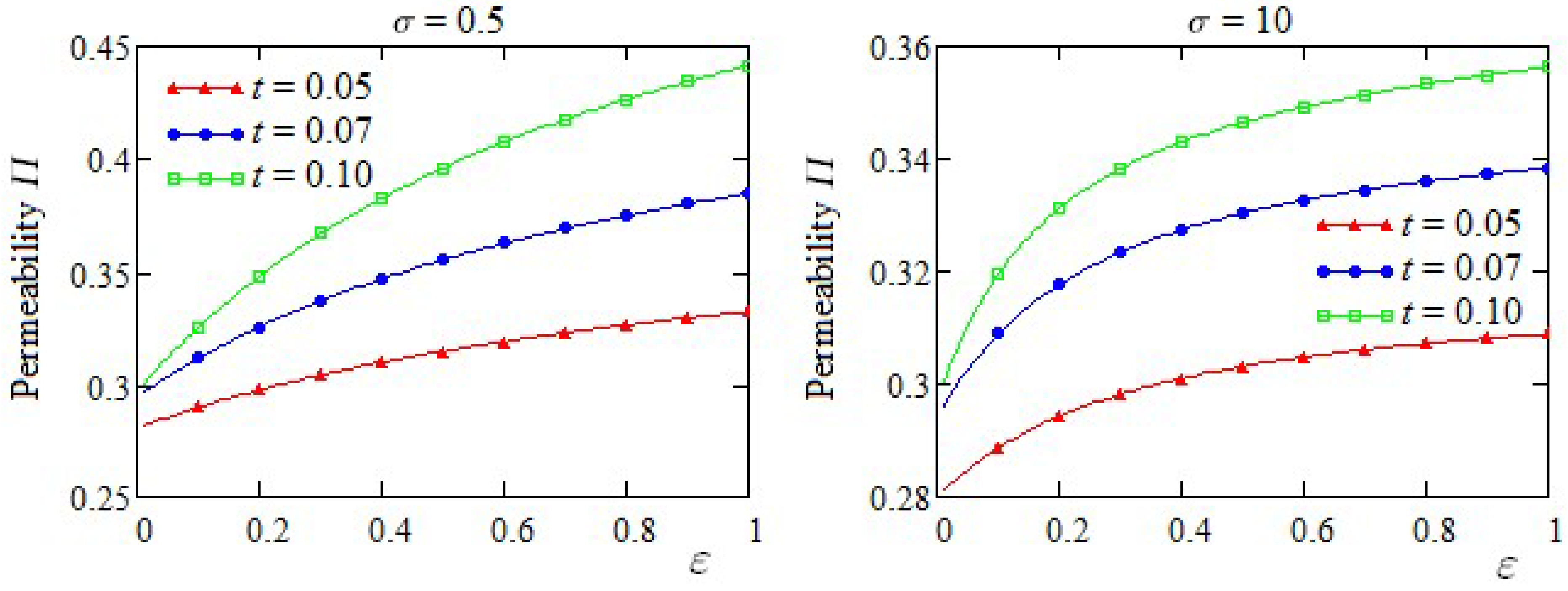
The influence of the local porosity $\epsilon$ of the porous medium on the hydrodynamic permeability is brought to light by the curves drawn in Figure 6 and Figure 7 for two values of the dimensionless permeability parameter $\sigma$ and different values of the time t. As expected, hydrodynamic permeability increases with the local porosity.

6. Conclusions

Transient axisymmetric flows of viscous fluids through an annular domain partly filled with a porous layer have been studied. The Brinkman equation for the flow inside the porous cylindrical shell and the Navier–Stokes equations outside the porous cylindrical region have been used.

Analytical solutions for velocity fields in the Laplace domain have been determined using Bessel functions, Laplace transform, and the appropriate interface and boundary conditions. A numerical algorithm for the Laplace transforms inversion has been used. In addition, the hydrodynamic permeability has been also determined.

The dependence of the velocity fields and of hydrodynamic permeability on the characteristic parameters of the porous layer has been analyzed by numerical simulations and graphical illustrations. It has been observed that hydrodynamic permeability is highly dependent on the properties of the porous medium.

It must be noted that, the velocity on the outer surface being given by an arbitrary function of time, the results in this paper could be used to study various filtration problems.

References

1. Darcy, H.P.G. Les Fontaines Publiques De La Ville De Dijon; Dalmont, V., Ed.; Scientific Research Publishing Inc.: Paris, France, 1856. (In French) [Google Scholar]
2. Brinkman, H.C. A calculation of the viscous force exerted by a flowing fluid on a dense swarm of particles. Appl. Sci. Res. 1949, 1, 27–34. [Google Scholar] [CrossRef]
3. Saxena, P.; Kumar, L. Flow of a viscous fluid through different porous structures embedded in porous medium. J. Porous Media 2012, 15, 1125–1135. [Google Scholar] [CrossRef]
4. Williams, W.O. Constitutive equations for flow of an incompressible viscous fluid through a porous medium. Q. Appl. Math. 1978, 36, 255–267. [Google Scholar] [CrossRef] [Green Version]
5. Hajipour, M.; Dehkordi, A.M. Transient behavior of fluid flow and heat transfer in vertical channels partially filled with porous medium: Effects of inertial term and viscous dissipation. Energy Convers. Manag. 2012, 61, 1–7. [Google Scholar] [CrossRef]
6. Khanukaeva, D.Y.; Filippov, A.N.; Yadav, P.K.; Tiwari, A. Creeping flow of micropolar fluid parallel to the axis of cylindrical cells with porous layer. Eur. J. Mech. B Fluids 2019, 76, 73–80. [Google Scholar] [CrossRef] [Green Version]
7. Farahani, S.D.; Majd, B.K.; Abed, A.M. Control of thermal and fluid flow characteristics of an oscillating cylinder by porous media. Alex. Eng. J. 2023, 65, 951–961. [Google Scholar] [CrossRef]
8. Deo, S.; Yadav, P.K.; Tiwari, A. Slow viscous flow through a membrane built up from porous cylindrical particles with an impermeable. Appl. Math. Model. 2010, 34, 1329–1343. [Google Scholar] [CrossRef]
9. Hussain, M.; Rasool, M.; Mehmood, A. Radiative flow of viscous nano-fluid over permeable stretched swirling disk with generalized slip. Sci. Rep. 2022, 12, 11038. [Google Scholar] [CrossRef]
10. Fengxia, L.; Fanhui, Z.; Yunqi, S.; Yu, Z. A fractal relative permeability model for two-phase flow through unsaturated shale porous medium. Front. Earth Sci. 2022, 10, 1009750. [Google Scholar] [CrossRef]
11. Shahnazari, M.R.; Moosavi, M.H.; Chamkha, A.J. Investigation of nonlinear fluid flow equation in a porous media and evaluation of convection heat transfer coefficient, by taking the Forchheimer term into account. J. Nanofluids 2022, 11, 598–603. [Google Scholar] [CrossRef]
12. Umavathi, J.C.; Sheremet, M.A. Chemical reaction influence on nanofluid flow in a porous layer: Stability analysis. Int. Commun. Heat Mass Transf. 2022, 138, 106353. [Google Scholar] [CrossRef]
13. Arpino, F.; Carotenuto, A.; Massaroti, N.; Mauro, A. New solutions for axial flow convection in porous and partly porous cylindrical domains. Int. J. Heat Mass Transf. 2013, 57, 155–170. [Google Scholar] [CrossRef]
14. Herrera-Hernandez, E.C.; Aguilar-Madera, C.G.; Espinosa-Paredes, G.; Hernandez, D. Modeling single-phase fluid flow in porous media through non-local fractal continuum equation. J. Eng. Math. 2023, 138, 8. [Google Scholar] [CrossRef]
15. Imani, C.; Mozafari-Shamsi, M. On the Magnus effect of a rotating porous circular cylinder in uniform flow: A lattice Boltzmann study. Phys. Fluids 2023, 35, 023608. [Google Scholar] [CrossRef]
16. Rashed, Z.Z. Impacts of the properties heterogeneity on 3D magnetic dusty nanofluids flow in porous enclosures with cylinders. Sci. Rep. 2022, 12, 9110. [Google Scholar] [CrossRef]
17. Dalabaev, U. Influence of the form of porous insert in the flow of a viscous liquid in a plane pipe. J. Appl. Math. Phys. 2022, 10, 372–378. [Google Scholar] [CrossRef]
18. Sedigh, K.M.; Gholamerza, I. Lattice Boltzmann study of fluid flow and heat transfer characteristics of a heated porous elliptic cylinder: A two-domain scheme. Int. J. Numer. Methods Heat Fluid Flow 2022, 33, 282–310. [Google Scholar]
19. Valdes-Parada, F.J.; Lasseux, D. Flow near porous media boundaries including inertia and slip: A one-domain approach. Phys. Fluids 2021, 33, 073612. [Google Scholar] [CrossRef]
20. Singh, S.K.; Verma, V.K. Exact solution of flow in a composite porous channel. Arch. Mech. Eng. 2020, 67, 97–110. [Google Scholar]
21. Reddy, N.K.; Sankar, M. Buoyant heat transfer of nanofluids in a vertical porous annulus: A comparative study of different models. Int. J. Numer. Methods Heat Fluid Flow 2023, 33, 477–509. [Google Scholar] [CrossRef]
22. Abate, J.; Valko, P.P. Multi-precision Laplace transform inversion. Int. J. Numer. Methods Eng. 2004, 60, 979–993. [Google Scholar] [CrossRef]
23. Valko, P.P.; Abate, J. Numerical inversion of 2-D Laplace transforms applied to fractional diffusion equation. Appl. Numer. Math. 2005, 53, 73–88. [Google Scholar] [CrossRef]
24. Nield, D.A.; Bejan, A. Convection in Porous Media; Springer: New York, NY, USA, 2014. [Google Scholar]
25. Debnath, L.; Bhatta, D. Integral Transforms and Their Applications, 2nd ed.; Chapman and Hall/CRC: New York, NY, USA, 2006. [Google Scholar]
26. Eiderman, V. An Introduction to Complex Analysis and the Laplace Transform; Chapman and Hall/CRC: New York, NY, USA, 2021. [Google Scholar]
27. Watson, G.N. A Treatise on the Theory of Bessel Functions, 2nd ed.; Cambridge University Press: Cambridge, UK, 1995. [Google Scholar]
28. Arfken, G.B.; Weber, H.J.; Harris, F.E. Mathematical Methods for Physicists: A Comprehensive Guide, 7th ed.; Elsevier: Amsterdam, The Netherlands; Academic Press: Cambridge, MA, USA, 2012. [Google Scholar]
Figure 1. Geometry of the flow.
Symmetry 15 00585 g001
Figure 2. Variation of the fluid velocity in the flow domain at different instants for the local porosity ε = 0.8 .
Symmetry 15 00585 g002
Figure 3. The influence of the dimensionless permeability parameter σ on the fluid velocity for ε = 0.8 and two values of the time t.
Symmetry 15 00585 g003
Figure 4. Variation of the hydrodynamic permeability with the parameter σ for small values of the time t.
Symmetry 15 00585 g004
Figure 5. Variation of the hydrodynamic permeability with the parameter σ for larger values of the time t.
Symmetry 15 00585 g005
Figure 6. Variation of the hydrodynamic permeability with the parameter ε for small values of the time t.
Symmetry 15 00585 g006
Figure 7. Variation of the hydrodynamic permeability with the parameter ε for larger values of the time t.
Symmetry 15 00585 g007
Disclaimer/Publisher’s Note: The statements, opinions and data contained in all publications are solely those of the individual author(s) and contributor(s) and not of MDPI and/or the editor(s). MDPI and/or the editor(s) disclaim responsibility for any injury to people or property resulting from any ideas, methods, instructions or products referred to in the content.