
Kant’s Modal Asymmetry between Truth-Telling and Lying Revisited


Instituto de Física de São Carlos, Universidade de São Paulo, Caixa Postal 369, São Carlos 13560-970, SP, Brazil
Symmetry 2023, 15(2), 555; https://doi.org/10.3390/sym15020555
Submission received: 6 February 2023
/
Revised: 15 February 2023
/
Accepted: 17 February 2023
/
Published: 20 February 2023
(This article belongs to the Special Issue Active Particle Methods toward Modelling Living Systems)
Abstract
:The modal asymmetry between truth-telling and lying refers to the impossibility of a world in which everyone lies, while on the contrary, a world in which everyone tells the truth is possible. This ethical issue is relevant to modern concerns about epistemic security, or the safety of knowledge. The breakdown of epistemic security leads to the erosion of trust and, hence, to an ‘impossible’ world since a willingness to believe in others is essential for the functioning of society. Here, we examine the threat of disinformation to epistemic security using an individual-based model in which individuals are both senders and receivers of signals and are characterized by their credulity and deceptiveness, which are targets of natural selection. The possible worlds are those favored by natural selection. Lies that significantly harm believers lead to the Kantian scenario: trust is completely eroded and the winners of the evolutionary race are incredulous. However, if the lies are not too harmful, our game evolutionary model predicts a world in which the individuals are both credulous and mildly untruthful. These two possible worlds are separated by a discontinuous phase transition in the limit of infinite population size.
1. Introduction
In this time of ‘alternative facts’, it seems fitting to bring Kant’s modal asymmetry between truth-telling and lying back into the limelight. Setting aside the evident moral distinction between lying and truthfulness, Kant (in his celebrated discussion of promise-keeping) claims that telling the truth is right and lying is wrong because lying cannot be universalized, whereas for truthfulness [1]:
For the universality of a law which says that anyone who believes himself to be in need could promise what he pleased with the intention of not fulfilling it would make the promise itself and the end to be accomplished by it impossible; no one would believe what was promised to him but would only laugh at any such assertion as vain pretense.
In other words, a world in which everyone tells the truth is possible, whereas one in which everyone lies is impossible [2]. This is perhaps the reason why the collapse of reliable sources of information and, hence, one’s ability to distinguish between truth and fiction (presented as truth) is considered a major problem today [3]. Without a common ground, it will not be possible to efficiently address the issues that threaten our world (e.g., global warming), which is likely to make our world literally ‘impossible’, not only in a philosophical sense.
This curious topic of ethical theory is then closely related to the present-day epidemics of disinformation, i.e., misinformation with the overt purpose of misleading [4,5], which threatens epistemic security [3]. Here, we quantitatively address this problem using an individual-based model in which the individuals are both senders and receivers of signals and each individual exhibits a credulity trait and a deceptiveness trait. We assume that trustfulness and lying are behaviors that evolve by natural selection. Hence, the possibility of a world in which individuals exhibit a certain combination of those traits is determined by the chances of such combination ending up as the winner of a game evolutionary race where all possible combinations are present at the onset of the competition. Of course, there is a big caveat here since, at least in humans, social interactions are not uniquely determined by genetic traits but are somehow conditioned by artifacts created by the social players [6,7]. We overlook these complications in order to keep the model simple. To give value to the signals, we assume that they represent the individual’s estimate of a property of the environment that is key to survival. If an individual chooses to ignore the signals exhibited by others, then it must find the truth by itself through the exploration of the environment, which poses its own risk.
We find that the outcome of the game evolutionary race depends on how harmful the lies are. On the one hand, lies that significantly reduce the chances of survival of the believers lead to the scenario described by Kant: trust is completely eroded and the winning combination of behavioral traits is total incredulity and any degree of deceptiveness. In fact, since the signals are ignored, it does not matter whether they are true or false. From the perspective of epistemic security, this result shows that disinformation can inhibit the capability of individuals to exchange information with one another, which is a catastrophic scenario for a social species. We stress that the impossibility of such a world is an exogenous factor since, as expressed in Kant’s quotation, the never-trust behavior is likely to be selected by natural selection. On the other hand, if the lies are not too harmful, our game evolutionary model predicts a world in which the individuals are both credulous and mildly untruthful. This is an interesting prediction, as a certain willingness to believe the information provided by others is essential for the functioning of society. Using finite size scaling, we show that these two possible worlds are separated by a discontinuous phase transition in the limit of infinite population size.
The remainder of the paper is organized as follows. In Section 2, we introduce the individual-based model and describe the interactions between the individuals and environment, as well as the interactions between pairs of individuals (e.g., through credulous and deceiving behaviors). Moreover, in this section, we describe the game evolutionary framework that enforces competition between individuals and determines the composition of future generations. In Section 3, we present the results of the individual-based simulations, focusing on the characterization of the credulity, deceptiveness, and viability of the winners of the evolutionary games. We summarize our findings by presenting scatter plots of the winners’ behavioral traits for a large number of independent runs and apply finite-size scaling [8,9] to show that there is a discontinuous phase transition separating the worlds of credulous and incredulous individuals. Finally, in Section 4, we review our main results and compare our approach with the active particle methods [10].
2. The Model
We consider a population of N individuals who are both senders and receivers of signals. Each individual exhibits a pair of traits. One trait—the credulity —governs the propensity of individual i to believe the information exhibited by its peers. The other trait—the deceptiveness —determines the propensity of individual i to lie about (or corrupt) the signals it exhibits [2]. In contrast to the economic [11] and evolutionary [12] theoretical approaches that assign arbitrary values to the payoff of each individual’s actions, here, we use an explicit model of the environment to determine the chances of survival (viability fitness) of the individuals.
Accordingly, the individuals must evaluate some aspect or property of the environment, which in some sense is key to their viability [13]. For instance, in the case of animal behavior [14], this property of the environment could be the amount of a food resource [15] or signals to migrate in seasonal migration [16]. In the case of epistemic communities [17,18,19], which is more relevant to our study, the property could be the truth of an assertion, e.g., the effect of human activity on global warming, the efficacy of vaccines, or the safety of electronic voting machines.
We assume that the individuals assess the key properties of the environment by sampling a normal distribution of mean and variance . The samples are the clues to the true value of that property, which we define as the mean of the normal distribution [13]. The viability of individual i is determined by the proximity of its estimate to the true value . More pointedly, the probability that individual i who sampled survives the environmental challenge is given by
The random variable is the viability or fitness of individual i, which is distributed by the probability distribution
for . The expected value of the survival probability is so that increasing the hazardousness of the environment (i.e., the difficulty of the challenge) makes it riskier for the individuals to find the answer themselves by directly exploring the environment. This is a nice feature of the model since is not too small, the individuals must resort to some sort of cooperation in order to survive the environmental challenge. We can set without loss of generality, as does not depend on .
For individual i, the alternative to exploring the environment is to copy the estimate from individual j (chosen randomly in the community). This happens with the probability given by the credulity of individual i. Of course, exploration of the environment happens with probability and consists of producing a new sample or, equivalently, a new viability using the probability distribution (2). It is implicit in our model that the individuals’ estimates are publicly displayed or exhibited without cost upon request.
However, individual j—the sender—exhibits a distorted form of its estimate of the true value with probability given by its deceptiveness . Copying this corrupted estimate results in the drop of the viability of individual i—the receiver—by an amount , where . Here, is the cost of credulity. In sum, by believing a sender of viability , the receiver may end up with viability with probability and viability with probability . Hence, for , the viability of the receiver is cut by half on average and for the lies are harmless. In Table 1, we offer a summary of the model parameters and their meanings.
Thus, and fully determine the behaviors of the individuals. Since our goal is to find out if there is an optimal behavior strategy to deal with the environmental challenges in a hazardous and socially unreliable scenario, we must allow individuals with different strategies to compete among themselves. This is achieved by considering an evolutionary game scenario [12], in which only the survivors have a chance to contribute offspring to the succeeding generation, who then face new environmental challenges themselves and so on. As already mentioned, surviving the environmental challenge is determined by the individual’s viability , and the number of survivors is usually significantly less than N. All survivors have the same probability to supply offspring to the succeeding generation in a process of repopulation that brings the population size back to the fixed value N. In other words, selection only works at the level of survival (viability selection) and not at the level of the (genetic) differences in the reproduction of survivors. Individual i can adopt four pure strategies, i.e., and (credulous and liar), and (credulous and truth-telling), and (non-trusting and liar), and and (non-trusting and truth-telling). In addition, it can infinitely adopt many mixed strategies characterized by non-extreme values of the credulity and deceptiveness parameters [11].
Next, we describe the rules that govern the evolutionary game scenario. At the initial generation , each individual is attributed a viability value according to the probability distribution (2), as well as uniformly distributed random values of the credulity and deceptiveness . We assume that all of these individuals pass to generation . Then we follow the steps:
- Each individual chooses independently whether to copy another individual, which happens with probability , or to explore the environment, which happens with probability . If individual i chooses to copy, then it selects at random one of the individuals in the population. For the sake of concreteness, let us assume that individual j is selected. Individual j then exhibits its original estimate of with probability and a distorted version with probability . In the former case, the viability of individual i becomes , whereas in the latter case, it becomes with . If individual i chooses to explore the environment, then it produces a fresh sample of the viability using the distribution (2). The viability types are updated simultaneously (parallel update).
- Each individual is put through the environmental challenge to decide whether it survives or not. Take, for instance, individual i with viability . We generate a random number and allow individual i to pass the challenge provided that . We recall that only the survivors have a chance to supply offspring to the succeeding generation (, in this case). All individuals are subjected to the environmental challenge simultaneously (parallel update).
- Generation is formed by picking N individuals at random with replacement among the survivors of the environmental challenge. These N individuals are the offspring of the survivors and this step resets the population size to N.
The situation is now similar to our point of departure, as we have N individuals that are uniquely identified by the viability , credulity , and deceptiveness for . Hence, we can repeat the above sequence of steps to obtain the population makeup at the subsequent generations until the fixation of a behavior strategy occurs [20]. By fixation, we mean that all N individuals become ‘genetically’ identical in the sense they are characterized by the same values of credulity and deceptiveness, although the viability may differ. In other words, all individuals share the same ancestor at generation , the winner of the evolutionary race [21]. Our goal is the characterization of this winner in terms of the control parameters of the model, i.e., N, , and .
Regarding the agent or individual-based modeling used in this study—this approach is the most natural for modeling and simulating a system of ’behavioral’ units and has been employed in a wide range of domains [22,23,24]. Its defining characteristic is microscopic modeling, as opposed to macroscopic modeling, which involves some coarse-graining of the microscopic variables and the possibility of describing the system using differential equations. Although agent-based modeling is straightforward to implement and could be considered more of a mindset than a technology [25], there are many toolkits and platforms available to assist with its implementation [26,27,28].
3. Results
In this section, we present and discuss the results of the simulations of the evolutionary game dynamics. We focus on the mean credulity of the population
the mean deceptiveness of the population
and the mean fitness of the population (or viability)
These quantities are measured before the environmental challenge and after the individuals have decided to copy others or explore the environment. At the point of measurement, the population consists of N individuals. For large N, we have and for . In this paper, we typically set . (The exception is in the analysis of the threshold phenomenon that requires an even larger N.) This relatively large population size is necessary to produce a representative sample of the two-dimensional space of the traits and when assembling the initial population.
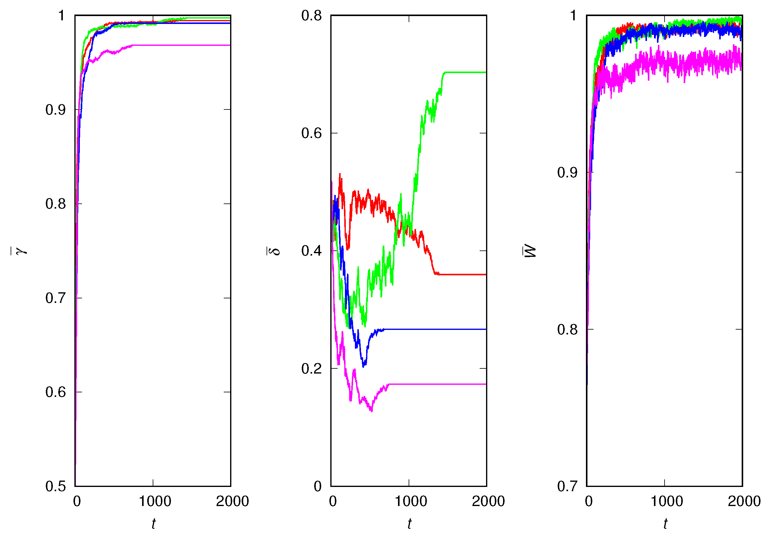
Figure 1 shows four independent runs for the case where the lies are harmless, i.e., for . More precisely, this is the case where even if the sender intends to lie, it ends up sending the correct signal. The winner in all runs is the extremely credulous strategy (), which guarantees almost certain survival (). Since the deceptiveness trait does not influence the fitness of the individuals, it drifts randomly until fixation is reached. After fixation, the population is homogeneous with respect to the traits and : all individuals are clones of the winner of the evolutionary race. Despite the population homogeneity, the mean fitness still fluctuates since some individuals choose to explore the environment and, hence, change their fitness. The fluctuations in the mean fitness disappear only if .
The reason it is advantageous to be credulous when the signals are always true is that believing unadulterated information is a safe wager; this is because the receiver obtains a viability that allows the sender lineage to survive at least one environmental challenge. The alternative is to gamble and generate viability ’afresh’ according to distribution (2), which has not yet been tested in an environmental challenge. This observation leads to the prediction that the uncertainty of the environment favors credulity.
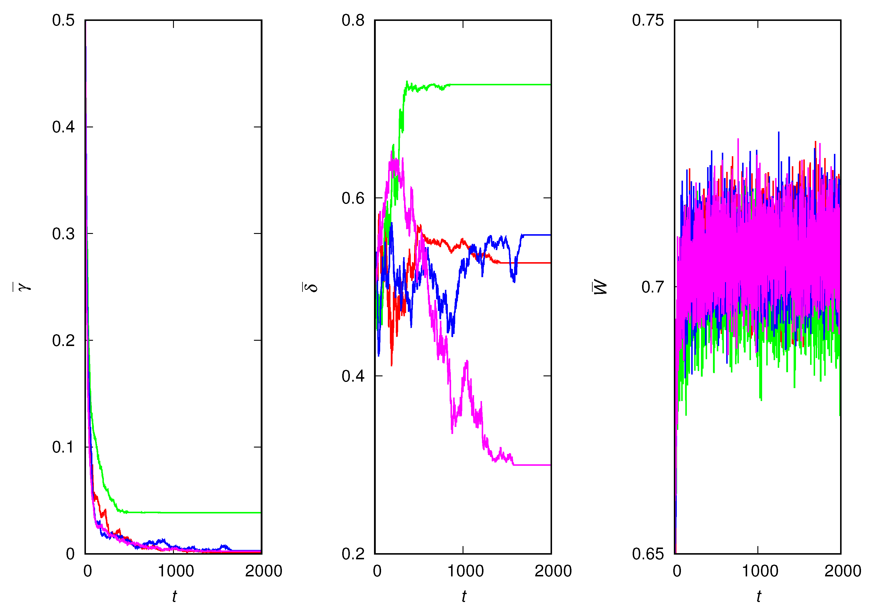
Figure 2 shows the results for the other extreme situation, for example, when the lies are the most harmful, i.e., . In this case, the receiver ends up with a viability that is half the viability of the sender on average. As expected, the winners are the most non-trusting individuals, who are very unlikely to copy their peers. Hence, it does not matter much whether the individuals are lying or not because nobody is listening anyway. This explains the random drift of the deceptiveness trait. Since the individuals are mostly sampling the environment, the mean population fitness is close to the expected value of distribution (2), which is for .
In the remainder of the paper, we will focus on the fixation (or equilibrium) regime only. As already pointed out, in this regime the population is characterized by the credulity and deceptiveness of the winner of the evolutionary game. However, unless the mean fitness of the population will continue to change even after fixation, as shown in Figure 1 and Figure 2. Therefore, to measure the mean fitness at equilibrium, we wait until fixation occurs and then average the mean fitness of the population over 100 generations.
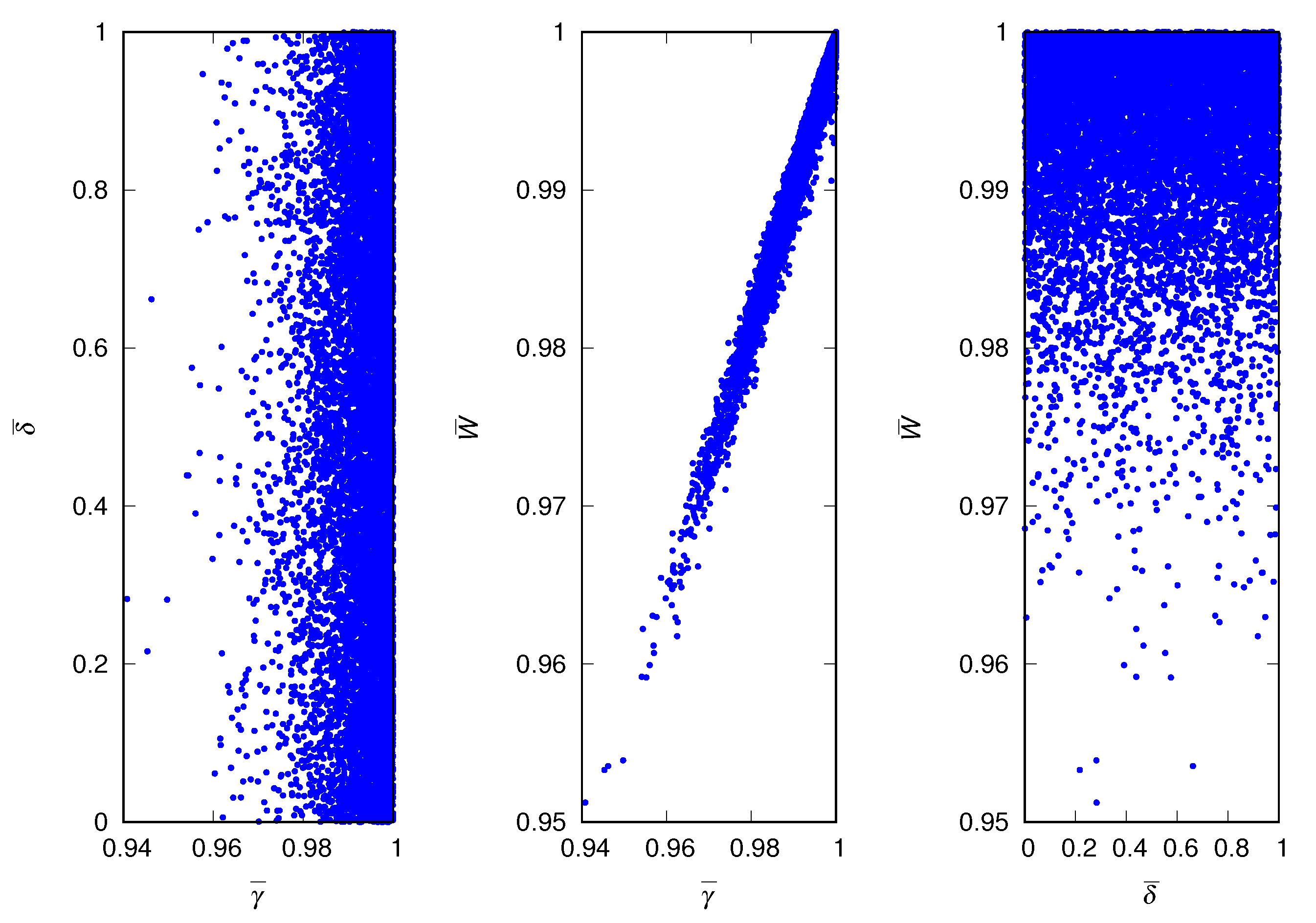
An instructive way to summarize the equilibrium properties of the population and visualize the variability between independent runs of the evolutionary dynamics is through scatter plots. Accordingly, in Figure 3 we present the scatter plots for the case of harmless lies (). Each symbol in the figure represents the equilibrium properties of the population for a particular run and the figure shows the results for independent runs. The results confirm that the four runs exhibited in Figure 1 are representative of the ensemble of runs. Since the deceptiveness trait does not influence the fitness of the individuals, the equilibrium value of is uniformly distributed in the unit interval . There is, however, a strong positive correlation between the credulity trait and the mean fitness of the population.
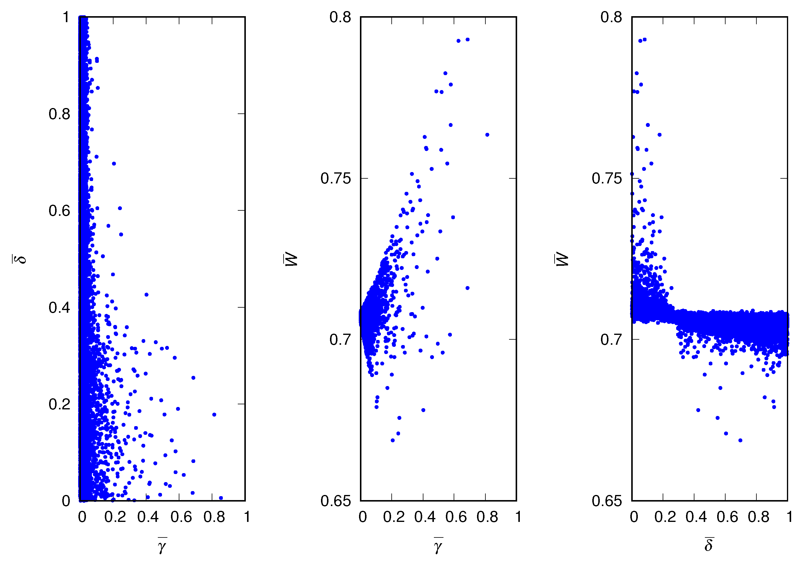
Figure 4 shows the scatter plots for the case . The winning strategies in most runs are characterized by low values of the credulity trait, which are expected in a situation where believing a corrupted signal may be very costly to the receiver. Although the mean deceptiveness of the population spans the entire unit interval, it is not uniformly distributed: there is a slight preference for low values of the deceptiveness trait. It is interesting that for , approximately, the strategy with the highest fitness is (never trust) which yields : all other strategies have lower fitness (see right panel of Figure 4).
In terms of maximizing the fitness of the population, the optimal scenario is a homogeneous population of credulous () and truth-telling () individuals, regardless of the values of the parameters and . However, despite their presence in the initial population, these altruistic individuals are quickly eliminated from the population by the liars and suspicious, resulting in a much lower mean fitness and, consequently, in the culling of a considerable fraction of the population at each generation (about of the data shown in Figure 4). Of course, this is an instance of the so-called Tragedy of the Commons [29,30], where the greedy determine the fate of the community.
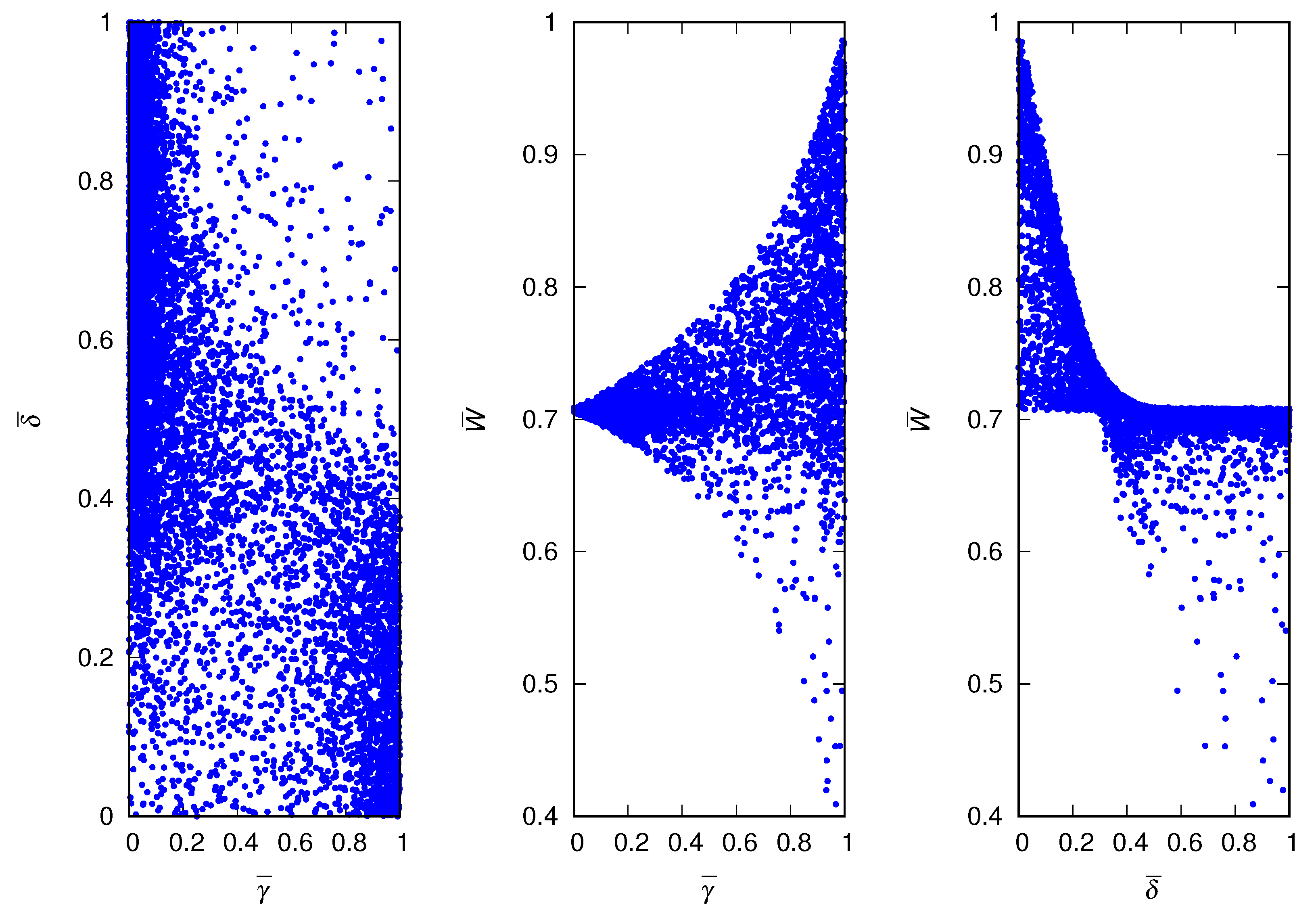
Before embarking on a more quantitative analysis of the winning strategies of the evolutionary game, we present in Figure 5 the scatter plots for an intermediate value of the credulity cost, i.e., . The results indicate the existence of two large clusters of winning strategies: low and medium to high , which has fitness less than , and high and low , which has fitness greater than . As expected, there are very few runs where the winners have high credulity and high deceptiveness. In fact, as a potentially winning strategy increases its frequency in the population, the individuals using the same strategy interact with each other more frequently leading to the extinction of the strategy in case of incompatible traits [31]. The two competing strategies identified by clusters in the scatter plots may be evidence of a discontinuous threshold phenomenon or phase transition [32], which is in fact the case, as we will show in the sequel.
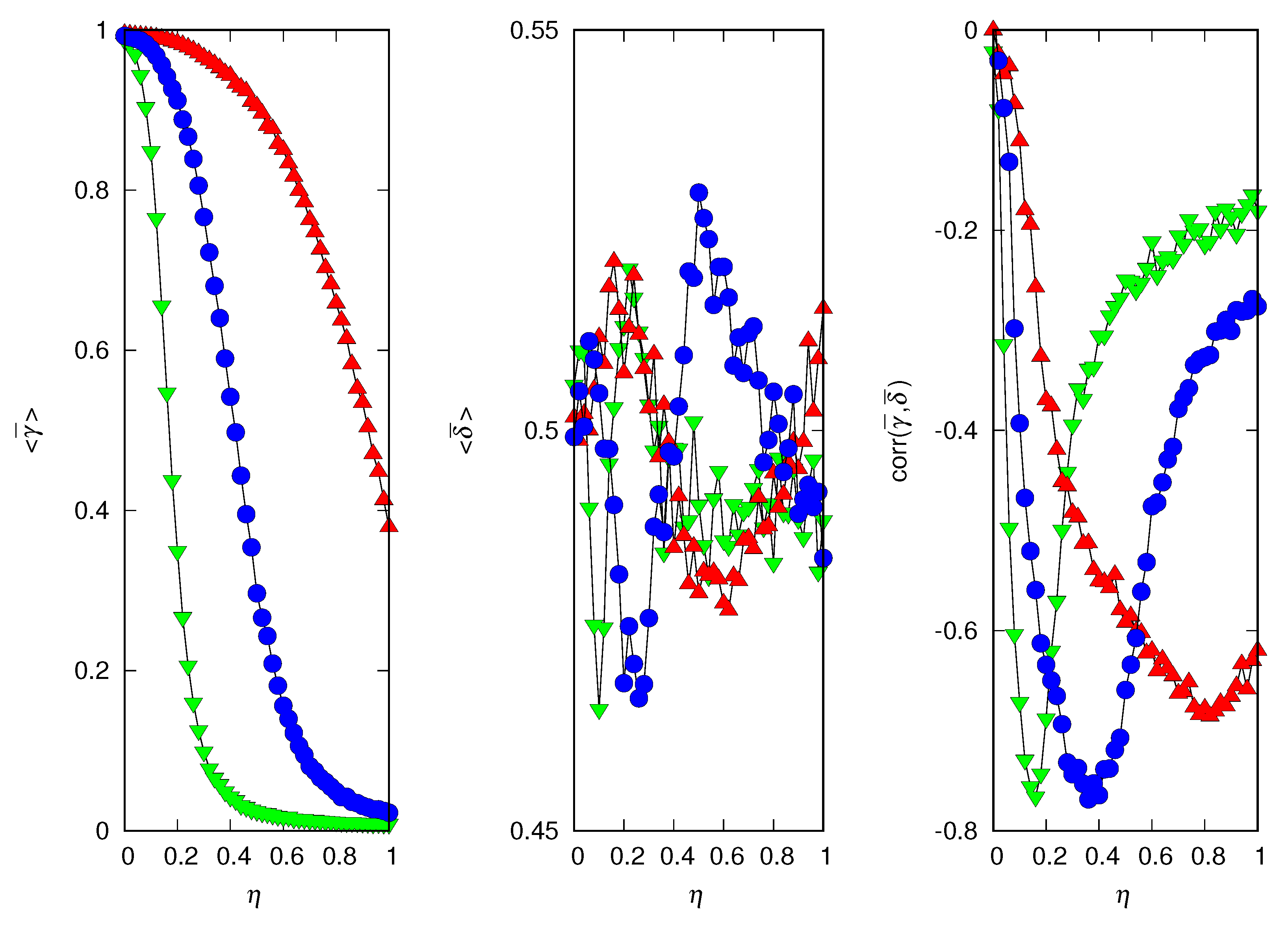
In Figure 6, we present the mean credulity and deceptiveness of the population averaged over 5000 independent runs, as well as the correlation between them. Henceforth, we will use the bracket notation to indicate the average over runs. The results indicate that increasing the cost of copying distorted information disfavors credulity, as expected. In addition, they indicate that an increase in the environment’s hazardousness favors credulity: if the risk of finding the answer by themselves is too high, the individuals are better off copying others, regardless of the cost involved in that decision. The mean deceptiveness of the population averaged over runs is much less informative because it does not vary significantly with or . In fact, the scatter plots of Figure 3, Figure 4 and Figure 5 indicate that the average over runs yields a value of close to despite the extreme variation of . The scale of the y-axis of the middle panel of Figure 6 is one-tenth of the scale of the left panel, hence the large fluctuations, but the intriguing oscillations are probably real. The correlation between and is always negative and its absolute value decreases in both extremes, and . In the former case, the lies are harmless, whereas in the latter case, most individuals are suspicious, so in both cases, it does not matter whether the individual is a liar or not (see Figure 3 and Figure 4). The minimum (or maximum in absolute value) of the correlation indicates a sharp separation between the two possible outcomes of the runs, i.e., winner i with high and low or winner i with low and medium to high .
Since a threshold phenomenon can happen only in systems of infinite size, , we have to resort to a finite size scaling analysis to determine whether our finite population results are indicative of such a phenomenon [8,9]. Figure 7 summarizes this analysis for .
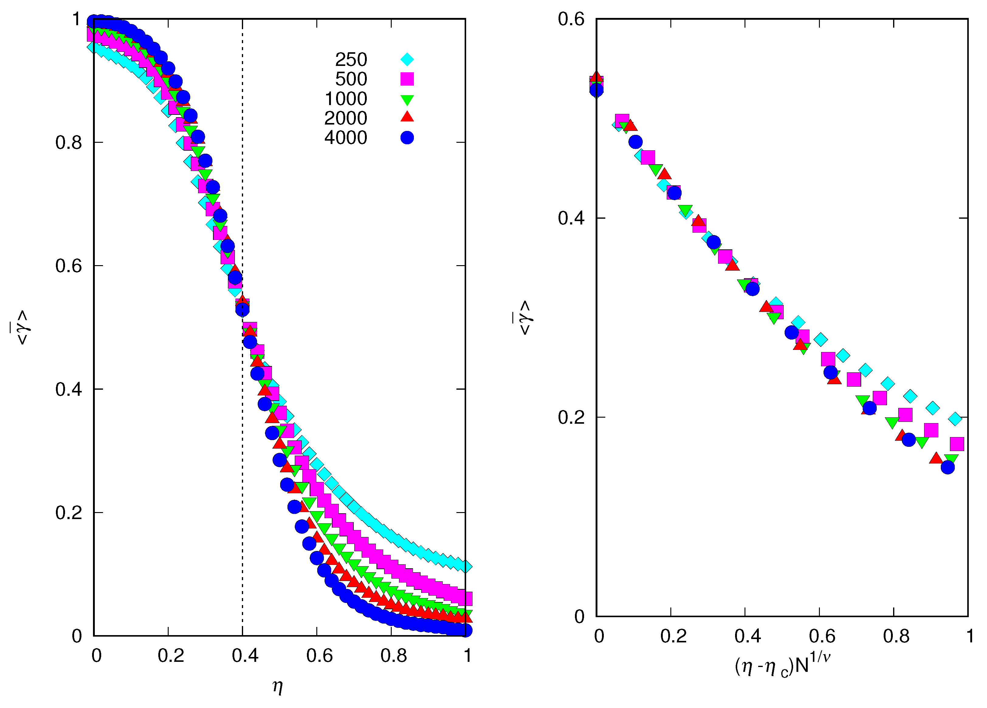
It is clear that for , with less than some critical value , the mean credulity of the population tends to a nonzero (and non-unit) value as the population size N increases. In fact, the results for and are practically indistinguishable in the left panel of Figure 7. However, for , the mean credulity of the population tends to zero with increasing N. So there is a discontinuous transition at , at which the mean credulity of the population jumps to zero, signaling the onset of a regime of complete incredulity on the truthfulness of the signals the individuals exhibit. We estimate by locating the values of at which the curves for different N intercept each other [8]. To quantify the sharpness of the transition for and finite but large N we use the scaling assumption [9]
where is a critical exponent and the scaling function is such that and . This means that for in the limit . At , Equation (6) implies that is invariant to changes in N; hence, the procedure to determine as the intersection of the curves vs. for different values of N. Of course, the validity of our scaling assumption (6) depends on whether we can determine the threshold and the critical exponent , such that the curves for different values of N ‘collapse’ into a unique curve, i.e., the scaling function [8,9]. In fact, the right panel of Figure 7 shows that the data collapse with and is very good, especially for the three largest population sizes.
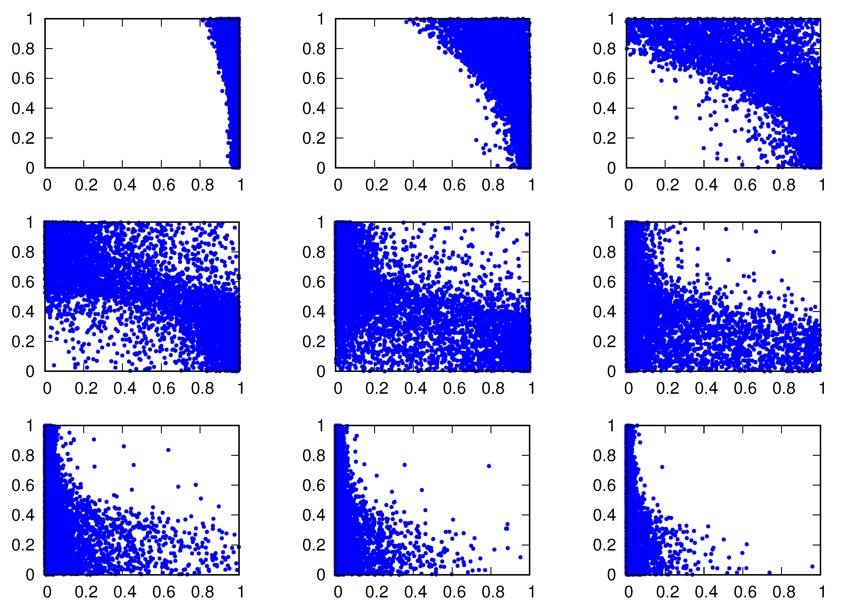
Figure 8 shows the two behavioral traits of the winning strategies in independent runs for several values of the credulity cost . We note that and are of little value to characterize the winning strategies, but the large negative values of the correlation between and signal the presence of two opposite attractors of the evolutionary dynamics at the discontinuous transition For instance, for we find = 0.53, = 0.49 and . As increases from to (the extremes and are shown in Figure 3 and Figure 4), we observe an increase in the number of runs for which the winners are highly untruthful but not too harmful because is small. As increases further, the individuals deal with untruthful and harmful signals by ignoring them, hence the increase in the number of runs for which the winners are highly incredulous.
4. Discussion
The conflict between lying and truth-telling is a well-established research topic both in biology and philosophy. For instance, the evolution of signals that are indicative of fitness and their selection for ‘honesty’ is a major issue in biology [33]. Regarding philosophy, Kant’s famous discussion of promise-keeping [1] leads to the view that a world in which everyone lies is unthinkable, not because it would be morally bad, but because such a world simply cannot exist. On the other hand, a world in which everyone tells the truth is possible [2]. Hence, the modal asymmetry between truth-telling and lying.
Our individual-based simulations offer some intriguing provisos to Kant’s conclusion. However, we must first interpret the existence of a world composed of individuals with a combination of credulity and deceptiveness, i.e., the possibility that such a combination ends up as the winner of a game’s evolutionary race where all possible combinations are present at the onset of the competition. Kant is correct in saying that if individuals only send untruthful signals, then no one would believe them and, hence, the very purpose of sending signals is lost. This is exactly the scenario we find when the cost of believing untruthful signals is higher than a threshold : trust is corroded and the winning strategy is extreme suspicion. From the perspective of epistemic security, this result shows that disinformation can erode trust and inhibit the capacity of the individuals to exchange information [3]. However, if (i.e., the lies are not too harmful) our game evolutionary model predicts a world in which the individuals are both very credulous and mildly untruthful.
An interesting feature of our model is that, as pointed out above, the winning strategies depend on the cost of believing corrupted information (or, on how harmful the lies are). Of course, the cost must be compared with the cost of ignoring the signals exhibited by others and finding the truth by oneself. Our model takes explicitly into account the risk of exploring the environment through the hazardousness and for too uncertain environments we find that it is always advantageous to be mildly credulous, regardless of the harmfulness of the lies (see data for in Figure 6). Thus, our model predicts that the more severe the environment is, the greater the credulity of the individuals.
The latest wave of authoritarianism, which is intimately related to disinformation, is perhaps a result of social disconnection and loneliness that were exacerbated by the COVID-19 pandemic [34,35,36]. In fact, in addition to being a major public health challenge [37], loneliness is a major social threat as shown by Hannah Arendt [38]:
The chief characteristic of the mass man is not brutality and backwardness, but his isolation and lack of normal social relationships.
It is tempting to relate this phenomenon to the predicted positive correlation between the hazardousness of the environment and the credulity of the individuals.
Our model builds on a previous, analytically solvable model that considers an infinite, homogeneous population with respect to credulity and deceptiveness, so there is no competition between distinct behavioral strategies [19]. In this case, the so-called winning strategy is chosen using a population-centered approach [39], where the optimal values of the parameters that determine the behavior of the individuals are chosen by maximizing the mean fitness of the population. As a result, the model predicts an artifactual regime (of extremely credulous () but deceptive () individuals) that does not appear in the present individual-based approach, where the individuals pursue their own interests.
To conclude, we will discuss the available mathematical approaches to modeling interacting living entities. Game theory has been the framework of choice to model decision-making problems in the economy and political sciences since von Neumann and Morgenstern’s landmark work [11]. A few decades later, Maynard Smith and Price showed how to use game theory to explain the logic of animal conflict [40] and since then this approach has been central to the mathematical modeling of the conflicting interactions between organisms, from humans to self-replicating molecules [41]. More recently, however, a novel mathematical framework has been developed to study the collective dynamics of large systems of interacting living entities—the active particle methods [10,42,43,44]. In this framework, at each interaction, individuals, viewed as active particles, play a game whose outcome is influenced by their strategies, which are usually associated with surviving and adaptive capabilities. The interactions between individuals, as well as between individuals and the environment, are described by theoretical tools of stochastic game theory. The strategies used by the individuals are heterogeneously distributed over the micro-states of players that encompass activity and mechanical variables. Individuals are represented by stochastic variables governed by a distribution function over the micro-state and the game payoff is heterogeneously distributed over individuals. The active particle methods have been applied to modeling a variety of systems, from economic and social problems [45] to the spreading of infectious diseases [46]. However, in contrast to the evolutionary game approach, the active particles methods are not easily grasped and implemented by non-mathematicians, hence our choice of the more conventional method to analyze a problem of interest to philosophy and social sciences, i.e., the modal asymmetry between truth-telling and lying.
Funding
This research was funded by Fundaç ao de Amparo à Pesquisa do Estado de S ao Paulo grant number 2020/03041-3 and Conselho Nacional de Desenvolvimento Científico e Tecnológico grant number 305620/2021-5.
Data Availability Statement
Not applicable.
Conflicts of Interest
The author declare no conflict of interest. The funders had no role in the design of the study; in the collection, analyses, or interpretation of data; in the writing of the manuscript; or in the decision to publish the results.
References
- Kant, I. Groundwork of the Metaphysics of Morals; Cambridge University Press: Cambridge, UK, 2012. [Google Scholar]
- Sober, E. The primacy of truth-telling and the evolution of lying. In From a Biological Point of View: Essays in Evolutionary Philosophy; Sober, E., Ed.; Cambridge University Press: Cambridge, UK, 1994; pp. 71–92. [Google Scholar]
- Seger, E.; Avin, S.; Pearson, G.; Briers, M.; Heigeartaigh, S.O.; Bacon, H. Tackling Threats to Informed Decision-Making in Democratic Societies; The Alan Turing Institute: London, UK, 2020. [Google Scholar]
- Fallis, D. Epistemic Values and Disinformation. In Virtue Epistemology Naturalized: Bridges between Virtue Epistemology and Philosophy of Science; Fairweather, A., Ed.; Springer: New York, NY, USA, 2014; pp. 159–179. [Google Scholar]
- Fallis, D. What Is Disinformation? Libr. Trends 2015, 63, 401–426. [Google Scholar] [CrossRef] [Green Version]
- Simon, H.A. A Formal Theory of Interaction in Social Groups. Am. Sociol. Rev. 1952, 17, 202–211. [Google Scholar] [CrossRef]
- Simon, H.A. The Sciences of the Artificial; MIT Press: Cambridge, UK, 1970. [Google Scholar]
- Binder, K. The Monte Carlo method for the study of phase transitions: A review of some recent progress. J. Comp. Phys. 1985, 59, 1–55. [Google Scholar] [CrossRef]
- Privman, V. Finite-Size Scaling and Numerical Simulations of Statistical Systems; World Scientific: Singapore, 1990. [Google Scholar]
- Burini, D.; Chouhad, N.; Bellomo, N. Waiting for a Mathematical Theory of Living Systems from a Critical Review to Research Perspectives. Symmetry 2023, 15, 351. [Google Scholar] [CrossRef]
- von Neumann, J.; Morgenstern, O. Theory of Games and Economic Behavior; Princeton University Press: Princeton, NJ, USA, 1944. [Google Scholar]
- Maynard Smith, J. Evolution and the Theory of Games; Cambridge University Press: Cambridge, UK, 1982. [Google Scholar]
- Agui naga, J.; Gomulkiewicz, R.; Watts, H.E. Effect of social information on an individual’s assessment of its environment. Anim. Behav. 2021, 178, 267–277. [Google Scholar] [CrossRef]
- Dall, S.; Giraldeau, L.-A.; Olsson, O.; McNamara, J.; Stephens, D. Information and its use by animals in evolutionary ecology. Trends Ecol. Evol. 2005, 20, 187–193. [Google Scholar] [CrossRef]
- Clark, C.W.; Mangel, M. Foraging and flocking strategies: Information in an uncertain environment. Am. Nat. 1984, 123, 626–641. [Google Scholar] [CrossRef]
- Fryxell, J.M.; Sinclair, A.R.E. Causes and consequences of migration by large herbivores. Trends Ecol. Evol. 1988, 3, 237–241. [Google Scholar] [CrossRef]
- Kitcher, P. The Advancement of Science: Science without Legend, Objectivity without Illusions; Oxford University Press: Oxford, UK, 1993. [Google Scholar]
- Reijula, S.; Kuorikoski, J. Modeling epistemic communities. In The Routledge Handbook of Social Epistemology; Fricker, M., Graham, P.J., Henderson, D., Pedersen, N.J.L.L., Eds.; Routledge: Abingdon, UK, 2019; pp. 240–249. [Google Scholar]
- Tórtura, H.A.; Fontanari, J.F. The synergy between two threats: Disinformation and COVID-19. Math. Models Methods Appl. Sci. 2022, 32, 2077–2097. [Google Scholar] [CrossRef]
- Crow, J.F.; Kimura, M. An Introduction in Population Genetics Theory; Harper and Row: New York, NY, USA, 1970. [Google Scholar]
- Serva, M. On the genealogy of populations: Trees, branches and offspring. J. Stat. Mech. 2005, 2005, P07011. [Google Scholar] [CrossRef]
- Gotts, N.; Polhill, J.; Law, A. Agent-based simulation in the study of social dilemmas. Artif. Intell. Rev. 2003, 19, 3–92. [Google Scholar] [CrossRef]
- Paulin, J.; Calinescu, A.; Wooldridge, M. Agent-based modeling for complex financial systems. IEEE Intell. Syst 2018, 33, 74–82. [Google Scholar] [CrossRef]
- Reia, S.M.; Amado, A.C.; Fontanari, J.F. Agent-based models of collective intelligence. Phys. Life Rev. 2019, 31, 320–331. [Google Scholar] [CrossRef] [PubMed] [Green Version]
- Bonabeau, E. Agent-based modeling: Methods and techniques for simulating human systems. Proc. Natl. Acad. Sci. USA 2002, 99, 7280–7287. [Google Scholar] [CrossRef] [PubMed] [Green Version]
- Nikolai, C.; Madey, G. Tools of the trade: A survey of various agent based modeling platforms. J. Artif. Soc. Soc. Simul. 2009, 12, 2. [Google Scholar]
- Macal, C.; North, M. Tutorial on agent-based modelling and simulation. J. Simul. 2010, 4, 151–162. [Google Scholar] [CrossRef]
- Cardinot, M.; O’Riordan, C.; Griffith, J.; Perc, M. Evoplex: A platform for agent-based modeling on networks. SoftwareX 2019, 9, 199–204. [Google Scholar] [CrossRef]
- Hardin, G. The Tragedy of the Commons. Science 1968, 162, 1243–1248. [Google Scholar] [CrossRef] [Green Version]
- Ostrom, E. Governing the Commons: The Evolution of Institutions for Collective Action; Cambridge University Press: Cambridge, UK, 1990. [Google Scholar]
- Axelrod, R. The Evolution of Cooperation; Basic Books: New York, NY, USA, 1984. [Google Scholar]
- Marro, J.; Dickman, R. Nonequilibrium Phase Transitions in Lattice Models; Cambridge University Press: Cambridge, UK, 1999. [Google Scholar]
- Zahavi, A. Mate selection—A selection for a handicap. J. Theor. Biol. 1975, 53, 205–214. [Google Scholar] [CrossRef]
- Fontanari, J.F. A stochastic model for the influence of social distancing on loneliness. Phys. A 2021, 584, 126367. [Google Scholar] [CrossRef]
- Hardy, P.; Marcolino, L.S.; Fontanari, J.F. The paradox of productivity during quarantine: An agent-based simulation. Eur. Phys. J. B 2021, 94, 40. [Google Scholar] [CrossRef] [PubMed]
- Fontanari, J.F. Productivity in Times of COVID-19: An Agent-Based Model Approach. In Predicting Pandemics in a Globally Connected World; Bellomo, N., Chaplain, M.A.J., Eds.; Springer: New York, NY, USA, 2022; Volume 1, pp. 213–231. [Google Scholar]
- Leigh-Hunt, N.; Bagguley, D.; Bash, K.; Turner, V.; Turnbull, S.; Valtorta, N.; Caan, W. An overview of systematic reviews on the public health consequences of social isolation and loneliness. Public Health 2017, 152, 157–171. [Google Scholar] [CrossRef] [PubMed] [Green Version]
- Arendt, H. The Origins of Totalitarianism; Mariner Books: Boston, MA, USA, 1973. [Google Scholar]
- Birch, J. Fitness Maximization. In The Routledge Handbook of Evolution and Philosophy; Joyce, R., Ed.; Routledge: Abingdon, UK, 2018; pp. 49–63. [Google Scholar]
- Maynard Smith, J.; Price, G.R. The Logic of Animal Conflict. Nature 1973, 246, 15–18. [Google Scholar] [CrossRef]
- Nowak, M.A. Evolutionary Dynamics: Exploring the Equations of Life; Harvard University Press: Cambridge, UK, 2006. [Google Scholar]
- Bellomo, N.; Bellouquid, A.; Gibelli, L.; Outada, N. A Quest towards a Mathematical Theory of Living Systems; Birkhäuser-Springer: New York, NY, USA, 2017. [Google Scholar]
- Bellomo, N.; Burini, D.; Dosi, G.; Gibelli, L.; Knopoff, D.A.; Outada, N.; Terna, P.; Virgillito, M.E. What is life? A perspective of the mathematical kinetic theory of active particles. Math. Models Methods Appl. Sci. 2021, 31, 1821–1866. [Google Scholar] [CrossRef]
- Bellomo, N.; Esfahanian, M.; Secchini, V.; Terna, P. What is life? Active particles tools towards behavioral dynamics in social-biology and economics. Phys. Life Rev. 2022, 43, 189–207. [Google Scholar] [CrossRef]
- Dolfin, M.; Leonida, L.; Outada, N. Modelling human behaviour in economics and social science. Phys. Life Rev. 2017, 22–23, 1–21. [Google Scholar] [CrossRef] [Green Version]
- Bellomo, N.; Bingham, R.; Chaplain, M.A.J.; Dosi, G.; Forni, G.; Knopoff, D.A.; Lowengrub, J.; Twarock, R.; Virgillito, M.E. A multiscale model of virus pandemic: Heterogeneous interactive entities in a globally connected world. Math. Models Methods Appl. Sci. 2020, 30, 1591–1651. [Google Scholar] [CrossRef]
Figure 1.
Four independent runs for harmless lies. (Left) Mean credulity of population against generation t. (Middle) Mean deceptiveness of population against generation t. (Right) Mean fitness of population against generation t. The parameters are , and .
Figure 1.
Four independent runs for harmless lies. (Left) Mean credulity of population against generation t. (Middle) Mean deceptiveness of population against generation t. (Right) Mean fitness of population against generation t. The parameters are , and .

Figure 2.
Four independent runs for the most harmful lies. (Left) Mean credulity of population against generation t. (Middle) Mean deceptiveness of population against generation t. (Right) Mean fitness of population against generation t. The parameters are , and .
Figure 2.
Four independent runs for the most harmful lies. (Left) Mean credulity of population against generation t. (Middle) Mean deceptiveness of population against generation t. (Right) Mean fitness of population against generation t. The parameters are , and .

Figure 3.
Scatter plots of equilibrium properties of the population for harmless lies. (Left) Mean credulity of the population and mean deceptiveness of the population. (Middle) Mean credulity of the population and mean fitness of the population. (Right) Mean deceptiveness of the population and mean fitness of the population. The parameters are , , and .

Figure 4.
Scatter plots of equilibrium properties of the population for the most harmful lies. (Left) Mean credulity of the population and mean deceptiveness of the population. (Middle) Mean credulity of the population and mean fitness of the population. (Right) Mean deceptiveness of the population and mean fitness of the population. The parameters are , , and .

Figure 5.
Scatter plots of equilibrium properties of the population for moderate lies. (Left) Mean credulity of the population and mean deceptiveness of the population. (Middle) Mean credulity of the population and mean fitness of the population. (Right) Mean deceptiveness of the population and mean fitness of the population. The parameters are , , and .

Figure 6.
Effect of the credulity cost for environment hazardousness (inverted triangles), 1 (circles) and 2 (triangles). (Left) Mean credulity of the population averaged over runs. (Middle) Mean deceptiveness of the population averaged over runs. (Right) Correlation between mean credulity and mean deceptiveness. The population size is . The lines connecting the symbols are guides to the eye.

Figure 7.
Finite-size scaling analysis of the threshold phenomenon for population sizes N = 250, 500, 1000, 2000, and 4000 as indicated. (Left) Mean credulity of the population averaged over runs against the credulity cost . The vertical dashed line indicates our estimate . (Right) Mean credulity of the population averaged over runs against the scaled credulity cost for . The environment hazardousness is .

Figure 8.
Scatter plots of the mean credulity of population (x axis) and mean deceptiveness of population (y axis) for (left-to-right, top-to-bottom) = 0.1, 0.2, 0.3, 0.4, 0.5, 0.6, 0.7, 0.8, and . The other parameters are and .
Figure 8.
Scatter plots of the mean credulity of population (x axis) and mean deceptiveness of population (y axis) for (left-to-right, top-to-bottom) = 0.1, 0.2, 0.3, 0.4, 0.5, 0.6, 0.7, 0.8, and . The other parameters are and .


Table 1.
Parameters of the model.
| Parameter | Meaning |
|---|---|
| N | population size |
| value of the key property of the environment | |
| hazardousness of the environment | |
| credulity of individual i | |
| deceptiveness of individual i | |
| cost of credulity |
Disclaimer/Publisher’s Note: The statements, opinions and data contained in all publications are solely those of the individual author(s) and contributor(s) and not of MDPI and/or the editor(s). MDPI and/or the editor(s) disclaim responsibility for any injury to people or property resulting from any ideas, methods, instructions or products referred to in the content. |
© 2023 by the author. Licensee MDPI, Basel, Switzerland. This article is an open access article distributed under the terms and conditions of the Creative Commons Attribution (CC BY) license (https://creativecommons.org/licenses/by/4.0/).
Share and Cite
MDPI and ACS Style
Fontanari, J.F. Kant’s Modal Asymmetry between Truth-Telling and Lying Revisited. Symmetry 2023, 15, 555. https://doi.org/10.3390/sym15020555
AMA Style
Fontanari JF. Kant’s Modal Asymmetry between Truth-Telling and Lying Revisited. Symmetry. 2023; 15(2):555. https://doi.org/10.3390/sym15020555
Chicago/Turabian StyleFontanari, José F. 2023. "Kant’s Modal Asymmetry between Truth-Telling and Lying Revisited" Symmetry 15, no. 2: 555. https://doi.org/10.3390/sym15020555
Note that from the first issue of 2016, this journal uses article numbers instead of page numbers. See further details here.