Thermodynamics of the Acceleration of the Universe in the κ(R, T) Gravity Model

Abstract

In this article, we examined the behavior of dark energy (DE) and the cosmic acceleration in the framework of $\kappa (R,T)$ gravity in the standard spherically symmetric coordinates $\left(x^i\right)$ = $t,r,\theta ,\varphi$, a spatially homogeneous and isotropic FLRW space–time. We discovered some remarkable cosmic characteristics in this investigation that are in line with both observations and the accepted $\mathsf{\Lambda }$CDM model. We made two assumptions in order to determine a deterministic solution of the modified field equations (MFEs): (i) $p=\gamma \rho$, where $\gamma (1\ge \gamma \ge 0)$ is a constant, (ii) $\mathsf{\Lambda }$ = $\beta H^2$, where $\beta$ is an arbitrary constant. We solved the MFEs and obtained the expression for the Hubble parameter. The depicted model of $\kappa (R,T)$ gravity was taken into consideration when discussing the behavior of the accelerating Universe. In $\kappa (R,T)$ gravity, the statefinder analysis was utilized to distinguish our model from the $\mathsf{\Lambda }$CDM model. The evolution of the cosmos was studied using an effective equation of state (EoS). We investigated the thermodynamic quantities and the generalized energy conditions in order to test the viability of our model. When dominant and weak energy conditions are satisfied, this validates the model; when the strong energy condition is not satisfied, this accelerates the expansion of the Universe.

1. Introduction

The accelerated expansion of the Universe at late times is probably the most-important unsolved problems in contemporary cosmology [1,2,3]. This means that around $70\%$ of the energy in the Universe must be in something called “dark energy”, which has a negative pressure. This is fully responsible for the acceleration phase of the Universe. The source and nature of DE would provide a significant aspect of a long-standing puzzle: the gravitational influence of the zero-point energies of particles and fields [4]. The most-crucial aspect of DE is that its energy content is either constant or significantly varies as the Universe expands. However, we do not precisely comprehend the nature of DE [5]. Conventionally, dark energy has been described by the equation of state (EoS) parameter $\gamma =\frac{p}{\rho }$, but this parameter should not be taken as a constant. From observational findings derived from SN-Ia data, we have $-1.67<\gamma <0.62$ [6]. In essence, $\gamma$ should not be treated as a constant. The EoS parameter has been considered as a constant in many theoretical investigations with values of $-1,0,1/3$ and $+1$ for vacuum-, dust-, radiation-, and stiff-fluid-dominated Universes, respectively. This is because there are not enough observational data to estimate the time variation of $\gamma$. This parameter is not always constant. The idea of “modified gravity” is very important because it can explain how galaxies spin and how galaxy clusters move in the Universe. Different types of modified gravity exist, including $f\left(R\right)$ [7,8], $f\left(T\right)$ [9], $f(R,T)$ [10,11,12], $f(R,G)$ [13], $f\left(G\right)$ [14,15], $f(T,B)$ [16,17], $f(Q,T)$ [18,19], $f\left(Q\right)$ [20,21], and $f(T,T_G)$ [22]. One “important class of these models includes $f\left(R\right)$ gravity models. The models with a nonminimal coupling between the scalar field and the curvature” are defined by the fact that the conformal metric transformation can be used to build mathematically equivalent general relativity (GR) models with a scalar field.

Modified theories of gravity provide another method for addressing the DE problem. The Einstein–Hilbert action in conventional GR may be extended to derive these modified theories. This concept gives rise to several alternative theories of gravitation, such as f($\tau$) gravity [23], f(R) gravity [24], and $f(R,T)$ gravity [25] (where R is the curvature scalar, $\tau$ is the torsion scalar, and T is the trace of the energy–momentum tensor). The reviews [26] provide a detailed analysis of modified gravity. In light of this, Teruel [27] proposed a new modified theory known as $\kappa (R,T)$ gravity. Specifically, “$\kappa (R,T)$ gravity is based on a natural extension of GR, where the modified field equations are produced by adding elements that contain just the scalar curvature R and the trace T of the stress-energy tensor”. Recently, the authors [28] addressed the issue of demonstrating cosmic acceleration in $\kappa (R,T)$ gravity. Here, a brief discussion of $\kappa (R,T)$ gravity, the accompanying field equations, and the essential conditions is provided [29].

The field equations derived from the aforementioned modified theories are far more difficult than GR. Additionally, during the modification process, some of the original theory’s subtlety is lost. In this context, Teruel [27] suggested that “the $\kappa (R,T)$ gravity theory, which is a non-Lagrangian modified gravity theory”. The least-action principle is a useful tool for creating physical theories, even though the gravitational theory put out in [29] is unrelated to it. The Einstein gravitational constant has a modification in $\kappa (R,T)$ that permits a moving gravitational constant. This strategy would require non-covariant conservation of the energy–momentum tensor, more like in previous modified gravity theories, such as Rastall gravity [30] and $f(R,T)$ gravity [10]. One of the most-effective methods for creating a physical theory and its potential generalizations is the least-action principle. We mention the direct application of symmetries and the development of general conservation laws among the many benefits of the Lagrangian formalism. However, there is no reason to assume that, in a final theory of Nature, common symmetries and/or normal conservation rules will always hold. In this regard, it is interesting to consider that Einstein did not initially derive general relativity (GR) using a variational principle [31,32]. Instead, he used a very different strategy to get to the right field equations, one that eventually worked by adding a trace term right in the field equations. The Einstein–Hilbert action (EHA), which is a variational principle, was discovered and added to the theory after the correct field equations had already been determined [33]. It is true that the equivalence principle and general covariance were the system’s founding notions. In a similar manner, Maxwell’s electrodynamics (ME), the other classical field theory, was not originally conceived of from any variational principle and was only established with the addition of a source term (the Maxwell displacement current) [34]. Both the GR and ME field equations were discovered without the use of a variational principle, which suggests that, perhaps, a new strategy might be considered. There is no justification to dismiss the quest for an alternate strategy that is distinct from the Lagrangian formalism in light of these historical events. This fact presents another significant justification for investigating a non-Lagrangian modified gravitational theory in this context. For a detailed discussion, the readers are advised to see [27].

According to [27], the $\kappa (R,T)$ modified gravity field equations are created by explicitly substituting new source terms in the GR-field equations.

$$R_{ij}-\frac{1}{2}R{g}_{ij}=\mathsf{\Lambda }{g}_{ij}+\kappa (R,T)T_{ij}$$

(1)

where “$g_{ij}$ is the metric potential”, $R_{ij}$ is the Ricci tensor, $\mathsf{\Lambda }$ is the “cosmological constant, $T_{ij}$ is the energy–momentum tensor and $\kappa (R,T)$ related to the Einstein gravitational constant”. It is considered as a function of the traces $T=g_{ij}{T}^{ij}$ and Ricci scalar $R=g_{ij}{R}^{ij}$. It is obvious that $\kappa$ depends on the scalars, so we must investigate the possibility of a variable gravitational constant. The field equation given by Equation (1) has no divergence on the left side.

$${▽}^j\left(\kappa (R,T)T_{ij}\right)=0$$

(2)

The non-covariant conservation of $T_{ij}$ is the foundation for these field equations, which may be defined as

$${▽}^j{T}_{ij}=\left(\frac{-{▽}^j\kappa (R,T)}{\kappa (R,T)}\right)T_{ij}$$

(3)

Two distinct options were examined together with their cosmological significance in [27]. The symbol for a matter–matter coupling is $\kappa \left(T\right)=-\lambda T+8\pi$ G, and a matter–curvature coupling is represented by $\kappa \left(R\right)=\alpha R+8\pi G$. In this context, it was assumed that the coupling constants $\lambda$ and $\alpha$ are modest and consistent with a small violation of the energy–momentum tensor. Investigating a flat $\kappa (R,T)$ gravity model and obtaining certain cosmological parameters were the aim of this article.

The paper is organized as follows: The introduction of $\kappa (R,T)$ is covered in Section 1. The formulation of $\kappa (R,T)$ gravity is discussed in Section 2. We discuss the various energy conditions in Section 3. Then, we check the evolutionary trajectory statefinder diagnostics in Section 4. The thermodynamics aspects are discussed in Section 5. We discuss the parametrization method to reconstruct the cosmological models under observational constraints in Section 6. Observational Hubble data and statistical methods used to constrain the model parameters are provided in Section 6.1. We analyze the Pantheon data with 1048 data points and the ${\chi }^2$ function in Section 6.2. Graphical representations are used to describe the many cosmological parameters, such as the DP, effective energy density, effective pressure, and EoS parameters. We also cover the energy conditions and statefinders under observational restrictions in this section. We outline our findings in the final Section 8.

2. Formulation of $\mathbf{\kappa }(\mathbf{R},\mathbf{T})$ Gravity

In this part of the article, we examine a Universe that is homogeneous and isotropic, and as a matter source, it is filled with a perfect fluid. The energy–momentum tensor can be written as follows:

$$T_{ij}=(p+\rho )u_i{u}_j-p{g}_{ij},$$

(4)

where p, $\rho$, and $u_i$ are the density, pressure, and four-velocity. In the standard spherically symmetric coordinates $\left(x^i\right)$ = $t,r,\theta ,\varphi$, a spatially homogeneous, isotropic, and flat Friedmann–Lemaitre–Robertson–Walker (FLRW) metric has the form:

$$d{s}^2=d{t}^2-\left[d{r}^2+r^{2}d{\theta }^2+r^{2}si{n}^2\theta d{\varphi }^2\right]a^2,$$

(5)

In this equation, $a\left(t\right)$ is the scale factor and r, $\theta$, and $\varphi$ are comoving spatial coordinates. Flat FLRW models have been remarkably successful in describing the observed nature of the Universe. These components allow two distinct modified Friedmann equations (MFEs) to be derived for $\kappa (R,T)$ [27]:

$$H^2=\frac{8\pi G}{3}\rho +\frac{\mathsf{\Lambda }}{3}-\frac{\lambda \rho }{3}(\rho -3p)$$

(6)

$$\dot{H}+H^2=-\frac{4\pi G}{3}(\rho +3p)+\frac{\mathsf{\Lambda }}{3}+\frac{\lambda }{6}({\rho }^2-9p^2).$$

(7)

Here, the Hubble parameter is defined as $H=\frac{\dot{a}}{a}$. We considered only the flat case suggested by observations [35], and we chose the function $\kappa (R,T)$ as $\kappa \left(T\right)=-\lambda T+8\pi G$, where ($8\pi G$ = $k_1$ = 1).

For the complete indeterminacy of the system, we considered a perfect gas equation of state:

$$p=\gamma \rho ,$$

(8)

where $0\le \gamma \le 1$ is an arbitrary constant.

The proportional importance of gravitational matter, which is defined by density $\rho$, decreases as the Universe expands, followed by $\mathsf{\Lambda }\simeq 3H^2$. We are already in a dark-energy-dominated Universe, so the relationship is already (nearly) true. Therefore, we considered the cosmological constant as

$$\mathsf{\Lambda }=\beta H^2,$$

(9)

where $\beta$ is the constant of proportionality. Beck [36] determined the explicit form of the cosmological constant, $\mathsf{\Lambda }=\frac{G^2}{{\hslash }^4}{\left(\frac{m_e}{\alpha }\right)}^6$, where $\alpha$ is the fine structure constant, G is the gravitational constant, ℏ is the reduced Planck constant, and $m_e$ is the electron mass. Accordingly, the (observable) vacuum energy density is given by [36] ${\rho }_{\mathsf{\Lambda }}$ = $\frac{c^4}{8\pi G}\mathsf{\Lambda }$= $\frac{G}{4\pi }\frac{c^4}{\hslash }{\left(\frac{m_e}{\alpha }\right)}^6$, where c is the speed of light. This formula produces the numerical value ${\rho }_{\mathsf{\Lambda }}\simeq 4.0961$ GeV/m${}^3$, which easily satisfies the present observational limitations [37]. For in-depth derivations, see [36]. In the literature (e.g., [38,39,40,41]), there exist some $\mathsf{\Lambda }\left(t\right)$ models already. However, most of them are written by hand, e.g., $\mathsf{\Lambda }\propto H^2$, $\mathsf{\Lambda }\propto \frac{\ddot{a}}{a}$, $\mathsf{\Lambda }\propto R$, $\mathsf{\Lambda }\propto {\rho }_m$, and $\mathsf{\Lambda }\propto {\alpha }^6$. Therefore, in this study, we considered a time-dependent $\mathsf{\Lambda }$.

Solving Equations (6) and (7) with the help of Equations (8) and (9), we obtain the Hubble parameter as (See Appendix A):

$$H=-\frac{2}{2c_1+(\beta -3)(1+\gamma )t}.$$

(10)

and the energy density as:

$$\rho =\frac{\sqrt{16{\pi }^2{G}^2-\frac{4(\beta -3)(3\gamma -1)\lambda }{(2c_1+(\beta -3)(\gamma +1)t){}^2}}-4\pi G}{(3\gamma -1)\lambda }.$$

(11)

The Hubble parameter $H\left(t\right)$ is large at early times. From Equation (10), we notice that $H\left(t\right)$ is decreasing as time is increasing. For $\gamma =0,1/3\mathrm{and}1$, $H\left(t\right)$ converges to finite values. Only the Hubble parameter, which is the inverse of time, has a dimension among the several cosmographic parameters.

In all of Figure 1, Figure 2, Figure 3, Figure 4, Figure 5 and Figure 6, in our derived model, we used the assumptions $\beta =1.5$ and $c1=0.5$. We determined that our model is stable for these values and that all cosmological parameters produce accurate results. As we can see from Equation (10), there are three possible values for the variable $\beta$: $\beta <3$, $\beta >3$, and $\beta =3$. We obtained H = constant for all time for $\beta =3$, which is inconsistent. If we used $\beta >3$, the model was unstable, and we did not achieve satisfactory results. The model was stable, and we obtain pretty good result when we took $\beta <3$ into account. $c_1$ being an arbitrary constant, we randomly selected a small value of $c_1=0.5$. In order to constrain the model parameter using OHD+ SN Ia (Pantheon) data, we additionally included Section 6 and Section 7 in the text. Here, $\beta =2.28$ was found, which is also less than three. The current cosmological observations are compatible with the situation of $\beta <3$. In this instance, we assessed every geometrical and physical parameter for eras where dust, radiation, and stiff matter predominated.

Integrating Equation (10), we obtain the scale factor as:

$$a\left(t\right)=c_2\left(2c_1+(\beta -3)(\gamma +1)t\right){}^{-\frac{2}{(\beta -3)(\gamma +1)}}.$$

(12)

where $c_1$ and $c_2$ are integrating constants.

One of the geometrical parameters, the deceleration parameter (DP), demonstrates the key to analyzing the dynamics of the Universe. The definition of the DP $q\left(t\right)$ is

$$q\left(t\right)=-\frac{a\ddot{a}}{{\dot{a}}^2}=-1-\frac{\dot{H}}{H^2}.$$

(13)

Now, we find the the value of q by using Equation (12), $\dot{a}\left(t\right)=\frac{da\left(t\right)}{dt}$, and we obtain the deceleration parameter $q\left(t\right)$ as

$$q=\frac{1}{2}t(2c_1+(\beta -3)(\gamma +1)t).$$

(14)

q plays a significant role in defining the essence of the models obtained in Figure 1. The deceleration parameter defines the difference between the actual age of the Universe and the Hubble time. The age of the Universe will be less than the Hubble time in a decelerating Universe with $q>0$ because it expanded more quickly in the past. In contrast, a Universe that has always expanded more quickly will have an age greater than the Hubble time. The Hubble time is the age of a Universe with q = 0, which is a constant rate of expansion. Recently, Dixit et al. [42] discussed the behavior of q for different numerical values of k and m. The model decelerates in a conventional manner when $q>0$. The model expands with acceleration when $-1<q\le 0$. The cosmos enlarges exponentially when $q=-1$ and super-exponentially when $q<-1$. For different values of $0\le \gamma \le 1$, the deceleration parameter in our derived model shows an accelerating phase. The background fluid was assumed to be the ideal fluid specified by Equation (4). Furthermore, we considered the scalar field to be solely a function of time. In terms of the effective energy density and pressure, the Friedmann equations for the generalized scalar–tensor theory are: $3H^2={\rho }_{eff}$, $3H^2+2\dot{H}=p_{eff}$, where ${\rho }_{eff}=\kappa \left(T\right)\rho +\mathsf{\Lambda }$ and $p_{eff}=-\kappa \left(T\right)p+\mathsf{\Lambda }$ [27]. Moreover, ${\rho }_{eff}$, and $p_{eff}$ are the effective density and effective pressure, respectively. By utilizing Equation (10) and the above condition, we derived the expressions for the effective energy density $\left({\rho }_{eff}\right)$ and effective pressure $\left(p_{eff}\right)$, which are obtained as:

$${\rho }_{eff}=\frac{\left(4\pi G-\sqrt{16{\pi }^2{G}^2-\frac{4(\beta -3)(3\gamma -1)\lambda }{(2c_1+(\beta -3)(\gamma +1)t){}^2}}\right){}^2}{(1-3\gamma ){\lambda }^2}+\frac{4\beta }{(2c_1+(\beta -3)(\gamma +1)t){}^2}$$

(15)

$$p_{eff}=\frac{\left(4\pi G-\sqrt{16{\pi }^2{G}^2-\frac{4(\beta -3)(3\gamma -1)\lambda }{(2c_1+(\beta -3)(\gamma +1)t){}^2}}\right){}^2}{(1-3\gamma ){\lambda }^2}-\frac{4\beta }{(2c_1+(\beta -3)(\gamma +1)t){}^2}$$

(16)

We observed that the effective energy density $\left({\rho }_{eff}\right)$ is decreasing as t is increasing For $\gamma =0$, $1/3$, and 1, and the effective energy density $\left({\rho }_{eff}\right)$ is positive throughout the evolution and approaches small positive values (see Figure 2a). In Figure 2b, we illustrate the behavior of the effective pressure $p_{eff}$. The effective pressure $p_{eff}$ is negative throughout the evolution for $(\gamma =1,1/3,0)$ and asymptotically approaches zero.

Equation of State Parameter

It was found that the EoS parameter depends on time. The EoS parameter can transit from $\omega >-1$ to $\omega <-1$ due to its time dependence [43]. If the EoS parameter is found to be $\omega <-1$, the phantom fluid dominates the Universe, and if the EoS parameter is found to be $-1<\omega <-1/3$, matter dominates the Universe. This suggests that a significant crunch could occur in the far future. The constraints of the EoS parameter of the DE model are provided by the Planck Collaboration [44] and WMAP group [45], which provide the ranges for the EoS parameter as $0.921\le \omega \le -1.26$ (Planck + WP + Union 2.1), $-0.89\le \omega \le -1.38$ (Planck + WP + BAO), and $-0.983\le \omega \le -1.162$ (WMAP + eCMB + BAO + H0). Additionally, it can be seen that the behavior of the model developed here is in good accordance with recent observational data [46]. The model lies in the phantom region, which is a DE-driven accelerated phase $\omega <-1$, and is in good agreement with the current observational data of the Universe [47]. By using Equations (15) and (16), we obtained the effective equation of state parameter as: ${\omega }_{eff}=\frac{{\rho }_{eff}}{p_{eff}}$.

$${\omega }_{eff}=\frac{\frac{\left(4\pi G-\sqrt{16{\pi }^2{G}^2-\frac{4(\beta -3)(3\gamma -1)\lambda }{(2c_1+(\beta -3)(\gamma +1)t){}^2}}\right){}^2}{(1-3\gamma ){\lambda }^2}+\frac{4\beta }{(2c_1+(\beta -3)(\gamma +1)t){}^2}}{\frac{\left(4\pi G-\sqrt{(16{\pi }^2{G}^2-\frac{4(\beta -3)(3\gamma -1)\lambda }{(2c_1+(\beta -3)(\gamma +1)t){}^2}}\right){}^2}{(1-3\gamma ){\lambda }^2}-\frac{4\beta }{(2c_1+(\beta -3)(\gamma +1)t){}^2}}$$

(17)

Reference [48] discussed the behavior of the equation of state parameter. The dust phase with $\gamma =0$ is one of the most-common phases seen with the EoS parameter. Then, $\gamma$ = 1/3 shows the phase where radiation is most important, while $\gamma$ = −1 shows the vacuum energy $\mathsf{\Lambda }$CDM model. Furthermore, the accelerating phase of the Universe, which is in recent discussion, is shown when $\gamma <-\frac{1}{3}$, which includes quintessence $(-1<\gamma$≤ 0) and the phantom regime ($\gamma <-1$). In our derived model, the EoS parameter lies in the quintessence region for $\gamma =1$; for $\gamma =0$, the EoS parameter lies in phantom region; for $\gamma =1/3$, this EoS approaches the $\mathsf{\Lambda }$CDM point (see Figure 3).

3. Generalized Energy Conditions

The energy requirements are very helpful for understanding classical GR, which determines the behavior of null, space-like, or time-like geodesics in the Universe and helps in understanding the singularity difficulties of space–time. The most-prevalent EC types are the strong energy conditions (SECs), null energy conditions (NECs), weak energy conditions (WECs), and dominant energy conditions (DECs). The ECs may be formulated in several ways, for example in a geometrical way, i.e., ECs are well-expressed involving the Ricci or Weyl tensors, in a physical way, i.e., the ECs are expressed purely through the stress–energy–momentum tensor, or in an effective way, i.e., the ECs can be expressed involving the energy density ($\rho$), which plays the role as the time-like component, and pressure p, which serves as the three-space-like component [49,50]. The best way to describe these four EC formulations is:

$$\begin{array}{ccc}& & \hfill \mathrm{Strong}\mathrm{energy}\mathrm{conditions}\left(\mathrm{SECs}\right)\mathrm{if}{\rho }_{eff}+3p_{eff}\ge 0;\hfill \\ & & \hfill \mathrm{Weak}\mathrm{energy}\mathrm{conditions}\left(\mathrm{WECs}\right)\mathrm{if}{\rho }_{eff}\ge 0,{\rho }_{eff}+p_{eff}\ge 0;\hfill \\ & & \hfill \mathrm{Null}\mathrm{energy}\mathrm{condition}\left(\mathrm{NECs}\right)\mathrm{if}{\rho }_{eff}+p_{eff}\ge 0;\hfill \\ & & \hfill \mathrm{Dominant}\mathrm{energy}\mathrm{conditions}\left(\mathrm{DECs}\right)if{\rho }_{eff}\ge 0,\left|p_{eff}\right|\le {\rho }_{eff}.\hfill \end{array}$$

By using Equations (15) and (16), we obtain

$${\rho }_{eff}+3p_{eff}=\frac{3\left(4\pi G-\sqrt{16{\pi }^2{G}^2-\frac{4(\beta -3)(3\gamma -1)\lambda }{(2c_1+(\beta -3)(\gamma +1)t){}^2}}\right){}^2}{(1-3\gamma ){\lambda }^2}-\frac{8\beta }{(2c_1+(\beta -3)(\gamma +1)t){}^2}$$

(18)

$${\rho }_{eff}=\frac{\left(4\pi G-\sqrt{16{\pi }^2{G}^2-\frac{4(\beta -3)(3\gamma -1)\lambda }{(2c_1+(\beta -3)(\gamma +1)t){}^2}}\right){}^2}{(1-3\gamma ){\lambda }^2}+\frac{4\beta }{(2c_1+(\beta -3)(\gamma +1)t){}^2}$$

(19)

$${\rho }_{eff}+p_{eff}=\frac{2\left(4\pi G-\sqrt{16{\pi }^2{G}^2-\frac{4(\beta -3)(3\gamma -1)\lambda }{(2c_1+(\beta -3)(\gamma +1)t){}^2}}\right){}^2}{(1-3\gamma ){\lambda }^2}$$

(20)

$${\rho }_{eff}-p_{eff}=\frac{8\beta }{(2c_1+(\beta -3)(\gamma +1)t){}^2}$$

(21)

The profiles of the ECs are shown in Figure 4a–d. In our derived model, the WECs, NECs, and DECs are satisfied (see

Table 1. The behavior of energy conditions for various limits of parameters $\gamma$ and $\lambda$.

Range of $\mathit{\lambda }$	$\mathit{\gamma }$	WECs	DECs	NECs	SCEs
−1.005	$(0,1/3)$	K = 3 $(0,1)$	K = 6 $(0,1.5)$	K = 0.7 $(0,1.8)$	K = 0.5 $(0,1.6)$
		$[3\downarrow 0]$$[1,10]$	$[6\downarrow 0]$$[1.5,10]$	$[0.7\downarrow 0]$$[1.8,10]$	$[0.5\downarrow -1.5]$$(1.6,2)$
					$[-1.5\uparrow 0]$$[2,10]$
−1.005	$(1/3,1)$	K = 0 $(0,1)$	K = 2.4 $(0,1.6)$	K = −0.03 $(0,1)$	K = −3 $(0,1.8)$
		K = 0.3 $(1,2)$	$[2.4\downarrow 0]$$[1.6,10]$	$[-0.03\uparrow 0]$$[1,10]$	$[-3\uparrow 0]$$[1.8,10]$
		$[0.3\downarrow 0]$$[2,10]$
0.010	$(0,1/3)$	K = 3 $(0,2)$	K = 6 $(0,1.5)$	K = 0.7 $(0,2)$	K = 0.5 $(0,1.7)$
		$[3\downarrow 0]$$[2,10]$	$[6\downarrow 0]$$[1.5,10]$	$[0.7\downarrow 0]$$[2,10]$	$[0.5\downarrow -1.5]$$(1.7,2)$
					$[-1.5\uparrow 0]$$[2,10]$
0.010	$(1/3,1)$	K = 0 $(0,0.7)$	K = 2.4 $(0,1.6)$	K = −0.3 $(0,1)$	K = −3 $(0,1.8)$
		K = 0.4 $(0.7,2)$	$[2.4\downarrow 0]$$[1.6,10]$	$[-0.3\uparrow 0]$$[1,10]$	$[-3\uparrow 0]$$[1.8,10]$
		$[0.4\downarrow 0]$$(2,10)$
1.005	$(0,1/3)$	K = 0 $(0.3,0.6)$	K = 6 $(0,1.5)$	K = 0.06 $(0,0.2)\cup (0.6,2)$	K = 0.5 $(0,1)$
		K = 0.8 $(0,0.3)\cup (0.6,2)$	$[6\downarrow 0]$ [1.5, 10]	$[0.6\downarrow 0]$ [2, 10]	$[0.5\downarrow -1]$$(1,2.5)$
		$[0.8\downarrow 0]$ [2, 10]			$[-1\uparrow 0.5]$$[2.5,10]$
1.005	$(1/3,1)$	K = 1 $(0,1.5)$	K = 2.4 $(0,1.6)$	K = −0.2 $(0,1.2)$	K = −3 $(0,1.8)$
		$[1\downarrow 0]$$[1.5,10]$	$[2.4\downarrow 0]$$[1.6,10]$	$[-0.2\uparrow 0]$$[1.2,10]$	$[-3\uparrow 0]$$[1.8,10]$

). The SECs are violated for $\gamma =0,1/3,1$. As a result, the validity of the NECs and $\rho >0$ together ensure the WECs and DECs. The negative behavior of the SECs demonstrates the accelerating expansion of the Universe [50].

4. Statefinder

The behavior of higher derivatives of the scale factor, other than H and q, is a crucial component that must be explained in order to fully comprehend the dynamics of the Universe. Due to these reasons, we generalized our domain to construct geometrical parameters that involve higher derivatives of a. Statefinder diagnostics is a method that takes into account a pair of geometric parameters ($r,s$) proposed by [51,52] to describe how different DE models work. The geometrical parameters that are utilized to evaluate and contrast various DE models are covered in this section. These parameters, ($r,s$), are described as

$$r=2q^2+q-\frac{\dot{q}}{H}$$

$$\begin{array}{ccc}\hfill & & \hfill r=\frac{1}{2}[t^2(2c_1+(\beta -3)(\gamma +1)t){}^2+t(2c_1+(\beta -3)(\gamma +1)t)\hfill \\ & & \hfill -((\beta -3)(\gamma +1)(-t)-2c_1)(c_1+(\beta -3)(\gamma +1)t)]\hfill \end{array}$$

(22)

$$s=\frac{1}{3}\left[\frac{r-1}{q-\frac{1}{2}}\right]$$

$$\begin{array}{ccc}\hfill & & \hfill s=\frac{1}{3\left(2c_{1}t+(\beta -3)(\gamma +1)t^2-1\right)}[t^2(2c_1+(\beta -3)(\gamma +1)t){}^2+t(2c_1+(\beta -3)(\gamma +1)t)+1\left)t\right)\hfill \\ & & \hfill +(c_1+(\beta -3)(\gamma (2c_1+(\beta -3)(\gamma +1)t)-2]\hfill \end{array}$$

(23)

The trajectories $(r,s)$, $(r,q)$, and $(s,q)$ are illustrated in Figure 5a–c, respectively. It is important to note that in, the $(r,s)$ plane, the point (1,0) represents the $\mathsf{\Lambda }$CDM model, $r>1$$s<0$ denotes a Chaplygin gas model, and $r<1$$s>0$ is the quintessence region. However, our model shows a behavior of CG at early times and approaches the $\mathsf{\Lambda }$CDM model at late times. Similarly, in the $(r,q)$ plane, the point (1, 0) indicates the $\mathsf{\Lambda }$CDM model. This trajectory is separated into two distinct areas. The region $r>1$, $q<-1$ on the $(r,q)$ plane shows the “phantom model”, whereas the region $r>1$, $q>-1$ shows the “quintessence” model [53].

In Figure 5c, q lies in a negative region and approaches the $\mathsf{\Lambda }$CDM point. Similarly, $(s,q)=(0,0)$ represents the $\mathsf{\Lambda }$CDM model. The purpose of these trajectories is to examine the convergence and divergence of parametric curves such as $(r,s)$, $(r,q)$, and $(s,q)$ with respect to the $\mathsf{\Lambda }$CDM model.

5. Thermodynamics

In this section, we consider the part of our analysis that has to do with thermodynamics. According to the second law of thermodynamics, the horizon’s entropy is always positive and increases with time in the Universe [54]. The energy in a comoving volume is $U=\rho V.$ The following equation describes how dissipative effects in a fluid with temperature $\mathcal{T}$ produce entropy $S_n$ in a comoving volume:

$$\begin{array}{c}\hfill \mathcal{T}{\dot{S}}_n=\dot{U}+p\dot{V}\end{array}$$

(24)

When a cosmic fluid’s energy density and pressure are entirely dependent on temperature, when the cosmic fluid has no net charge, we obtain easily [28]

$$\begin{array}{c}\hfill S_n=\frac{V}{\mathcal{T}}(\rho +p)\end{array}$$

(25)

For a fluid whose equation of state is given by $p=\gamma \rho$, Equation (25) reduces to

$$\begin{array}{c}\hfill S_n=\frac{(1+\gamma )\rho V}{\mathcal{T}}\end{array}$$

(26)

where $0<\gamma <1$.

Now that we have determined the entropy density in terms of temperature, the first law of thermodynamics can be stated as

$$\begin{array}{c}\hfill S_d=\frac{S_n}{V}=\frac{(1+\gamma )\rho }{\mathcal{T}}.\end{array}$$

(27)

It expresses the entropy density as a function of temperature. The first law of thermodynamics is expressed as

$$\begin{array}{c}\hfill d\left(\rho V\right)+\gamma \rho dV=(1+\gamma )\mathcal{T}d\left(\frac{V\rho }{\mathcal{T}}\right).\end{array}$$

(28)

Integrating Equation (28), we obtain

$$\begin{array}{ccc}\hfill & & \hfill \mathcal{T}={\rho }^{\frac{\gamma }{1+\gamma }}\hfill \end{array}$$

(29)

From Equations (27) and (29), one can obtain

$$\begin{array}{ccc}\hfill & & \hfill S_d=(1+\gamma ){\rho }^{\frac{1}{1+\gamma }}\hfill \end{array}$$

(30)

Accordingly, the entropy of a comoving volume varies:

$$\begin{array}{ccc}\hfill & & \hfill S_n\sim S_{d}V\hfill \end{array}$$

(31)

These equations are invalid for a vacuum fluid with $\gamma =-1$. For a Zel’dovich fluid $(\gamma =1)$, we obtain:

$$\begin{array}{ccc}\hfill & & \hfill \mathcal{T}\sim {\rho }^{\frac{1}{2}}\mathrm{and}{S}_n\sim {\rho }^{\frac{1}{2}}\hfill \end{array}$$

(32)

Using Equations (10) and (13) in Equations (29) and (30), we find, respectively, the temperature $\left(\mathcal{T}\right)$ and entropy density $\left(S_d\right)$ as

$$\begin{array}{c}\hfill \mathcal{T}=\left(\frac{\left(4\pi G-\sqrt{16{\pi }^2{G}^2-\frac{4(\beta -3)(3\gamma -1)\lambda }{(2c_1+(\beta -3)(\gamma +1)t){}^2}}\right){}^2}{(1-3\gamma ){\lambda }^2}\right){}^{\frac{\gamma }{\gamma +1}}\end{array}$$

(33)

$$\begin{array}{c}\hfill S_d=(1+\gamma )\left(\frac{\left(4\pi G-\sqrt{(16{\pi }^2{G}^2-\frac{4(\beta -3)(3\gamma -1)\lambda }{(2c_1+(\beta -3)(\gamma +1)t){}^2}}\right){}^2}{(1-3\gamma ){\lambda }^2}\right){}^{\frac{1}{\gamma +1}}\end{array}$$

(34)

From Figure 6a, it is clear that the temperature for our model is a decreasing function of time. The model therefore satisfies the second law of thermodynamics. From Equation (34), we see that the rate of change of entropy with time is positive (see Figure 6b). This also implies that the entropy decreases over time. This conforms well with the second law of thermodynamics.

6. Cosmological Model with Observational Constraints

In this part, we implement the parametrization approach to reconstruct the cosmological models. For example, one may find a fascinating research work in which they employed the parametrization approach to investigate cosmological models. The primary benefit of using this method is that we can explore cosmological theories using observable data. The relationship between the scale factor a(t) and the redshift z is $1+z=a_0/a$, where $a_0$ is the late-time scale factor. From the above relation, we can find $\frac{d}{dt}=-H(1+z)\frac{d}{dz}$. To describe the dynamics of the Universe, the Hubble parameter H in terms of redshift can be written as

$$H\left(z\right)=H_0{(1+z)}^{\frac{(3-\beta )(\gamma +1)}{2}}$$

(35)

where $H_0$ is the present value of $H\left(z\right)$ and $\beta$ is the free parameter. In order to describe the dynamical and physical properties of the model with redshift, we considered $\gamma =1$ for the stiff fluid model to describe the behavior of the Universe. In this context, we discuss two observational datasets in the following section.

6.1. Observational Hubble Data

The observational data and statistical techniques used to constrain the model parameters of the derived Universe are described in this subsection. We used “57 $H\left(z\right)$ observational data point ranges $0\le z\le 2.36$ acquired using the Markov Chain Monte Carlo (MCMC) technique”.

The ${\chi }^2$ statistic was used to determine the best-fitting values and limits for a fitted model [55]. The estimated values of were $H_0=61.5_{-2.4}^{+2.7}$ kms${}^{-1}$ Mpc${}^{-1}$ and $\beta =1.{981}_{-0.084}^{+0.087}$. In order to limit the model’s parameters $H_0$ and $\beta$, we define ${\chi }^2$ as

$${\chi }^2\left(H_0,\beta \right)=\sum _{i=1}^{57}\frac{{\left(H_{th}\left(i\right)-H_{ob}\left(i\right)\right)}^2}{\sigma {\left(i\right)}^2}$$

(36)

where “$H_{th}\left(i\right)$” is the theoretical value of “H(z), and ${\sigma }_i$’s” is the error in the observed value of “H(z)”. With confidence levels of 68.3 %, 95.4 %, and 99.7%, we were able to obtain the 1D marginalized distribution and 2D contours for our model, which are shown in Figure 7 and Figure 8.

6.2. Pantheon Data

The pantheon data are the most-important observational datasets, with 1048 data points, and are the most-comprehensive known SNe Ia records. Pantheon datasets include points that spectroscopically cover the region of redshift z between $z=$ (0.01, 2.26).

The ${\chi }^2$ function for the Pantheon sample of 1048 SNe Ia reads as

$${\chi }^2(H_0,\beta )=\sum _{i=1}^{1048}\frac{{[{\mu }_{th}\left(\mathrm{z}(H_0,\beta ,z_i)\right)-{\mu }_{obs}\left(z_i\right)]}^2}{\sigma {\left(i\right)}^2}$$

(37)

“${\mu }_{obs}$ and ${\mu }_{th}$ are represents as the observed and theoretical distance modulus. $\sigma \left(i\right)$ denotes the standard error of the observed values”. We fit the free parameters of our model by comparing ${\mu }_{obs}$ with the observational values ${\mu }_{th}$ of the distance modulus. The distance model can be obtained by the equation ${\mu }_{th}=\mu \left(D_L\right)=m-M=5lo{g}_{10}\left(D_L\right)+{\mu }_0$. The associated terms $M,m$ and ${\mu }_0$ are represented as the absolute magnitude, apparent magnitude, and marginalized nuisance parameter. Furthermore, ${\mu }_0$ can be obtained as ${\mu }_0=5log(H_0^{-1}/Mpc)$$+25$ (see Figure 9) [56].

We summarize the numerical result of the statistical analysis in

Table 2. The results are summarized for the parameters of $H\left(z\right)$, $Pantheon$, and $H\left(z\right)+Pantheon$.

Data	${\mathit{H}}_0$	Model Parameter ($\mathit{\beta }$)t
$H\left(z\right)$	$61.5_{-2.4}^{+2.7}$	$1.{981}_{-0.084}^{+0.087}$
$Pantheon$	$73\pm 2.1$	$2.{96}_{-0.99}^{+0.86}$
$H\left(z\right)+Pantheon$	$69.3\pm 1.7$	$2.{289}_{-0.033}^{+0.036}$

. We can test the predictions of our theory with the available data by implementing the MCMC process.

7. Cosmological Parameters

The deceleration parameter $q=-1+\frac{(1+z)}{H\left(z\right)}\frac{dH}{dz}$ is one of the cosmological parameters that plays a vital role in understanding the current condition of the expansion of our Universe. When the value of the deceleration parameter is strictly less than zero, it demonstrates the accelerating behavior of the Universe; however, when the value of the parameter is not strictly less than zero, it demonstrates that the cosmos is decelerating. In addition, all of the observational evidence (OHD, Pantheon, OHD + Pantheon) demonstrates that our present Universe is in an accelerating phase for $\gamma =1$. This is the case since $\gamma =1$ denotes the acceleration of the expansion of the Universe (see Figure 10a).

Figure 10b shows that there is an increase in the energy density of the Universe with a redshift, and this trend appears to be continuing as the Universe expands. On the other hand, Figure 10c shows that there is a decrease in pressure with redshift, and this pressure has large negative values throughout the course of cosmic evolution. The EoS parameter, known as ${\omega }_{eff}$, may also be used to classify the decelerating and accelerating behavior of the Universe, and its definition is as follows: ${\omega }_{eff}=\frac{p_{eff}}{{\rho }_{eff}}$. After examining Figure 10d, we found that ${\omega }_{eff}=-3.001$ for OHD, ${\omega }_{eff}=-1.024$ for Pantheon, and ${\omega }_{eff}=-1.864$ for OHD + Pantheon are the current values of the EoS parameter and that ${\omega }_{eff}<0$. Our result aligns with some of the studies [57], which indicates an accelerating phase.

7.1. Energy Conditions

Figure 11 depicts the profile of the energy density, WECs, NECs, DECs, and SECs in relation to redshift z. We can see from the figure that the WECs and DECs are satisfied, whereas the NECs and SECs are violated. This is in agreement with the present scenario of the Universe. These features led us to the conclusion that every behavior shows an accelerating expansion of the cosmos.

7.2. Statefinders

Many trajectories in the $(r-s)$, $(r-q)$, and $(s-q)$ planes show the chronological evolution of several dark energy concepts. A few fixed point in these planes are $(r,s)=(1,0)$ and $(r,q)=(1,-1)$ for $\mathsf{\Lambda }$CDM shown in the $(r,s)$ plane, and $(r,q)$ and $(s,q)$ have a large deviation from the $\mathsf{\Lambda }$CDM model in the future (see Figure 12).

8. Conclusions

This article focused on the $\kappa (R,T)$ gravity model. The deterministic solutions of the $\kappa (R,T$) field equations were derived by considering the $p=\gamma \rho$. We examined the cosmological parameters such as the energy density, pressure, EoS, deceleration, Hubble, and cosmological planes such as statefinder trajectories $(r,s)$, $(r,q)$, and $(s,q)$. We also discussed the Universe’s thermodynamic behavior.

The characteristics of the derived model were examined using appropriate model parameter values. Our findings are summarized below:

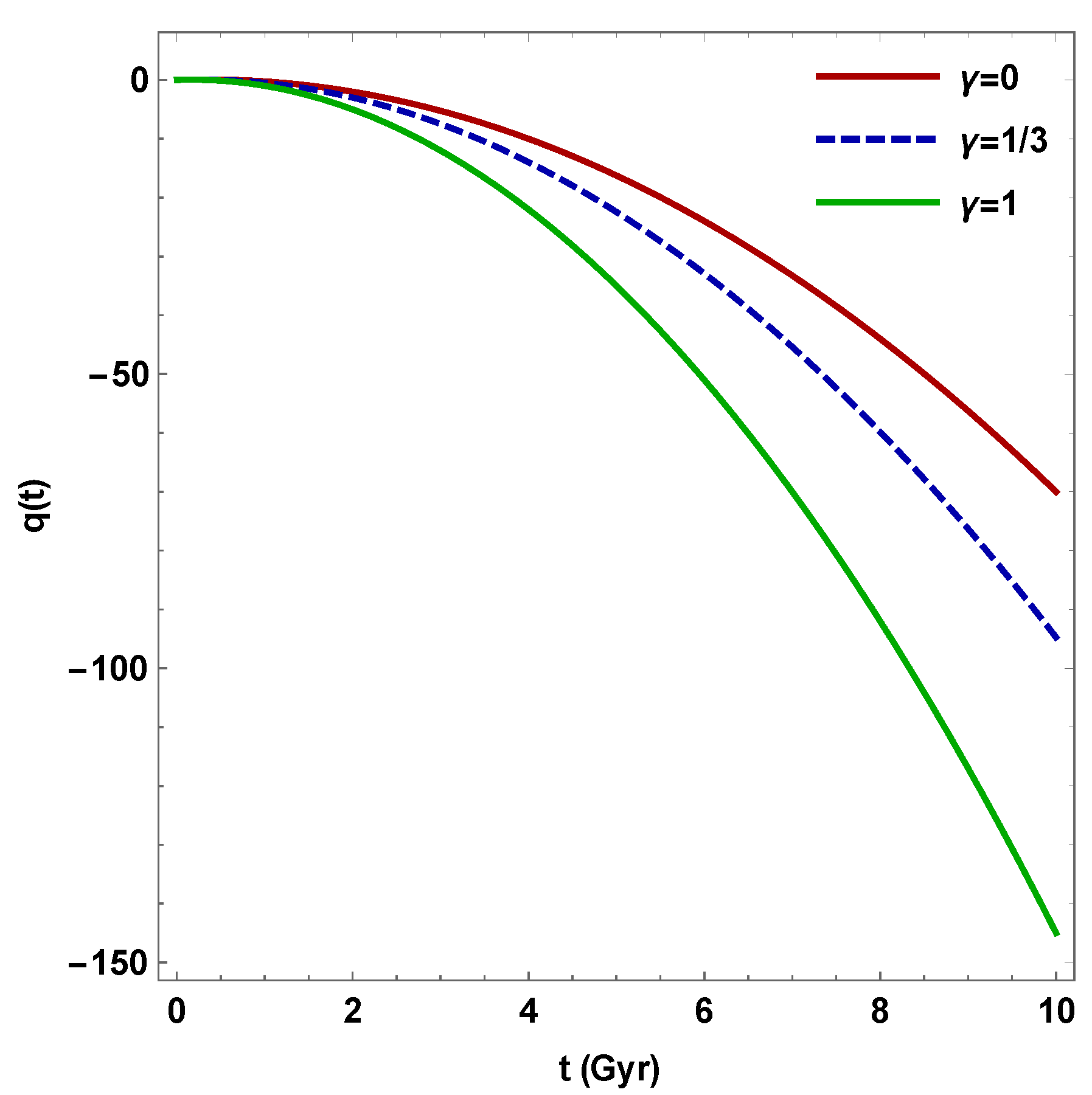
• We examined how much the DP reveals about the current acceleration of the Universe. The Hubble parameter $\left(H\right)$ and the DP $\left(q\right)$ are crucial parameters that may be utilized to describe the geometrical characteristics of the cosmos. Since $a>0$, the expansion of the cosmos is symbolized as $H>0$. The evolution of q versus t is depicted in Figure 1. Our model lies in an accelerating phase at present.
• During the cosmic evolution, the effective energy density ${\rho }_{eff}$ is positive and declines with time (see Figure 2a). However, we can observe that the effective pressure p is always negative for various $\gamma$ values throughout the development (see Figure 2b).
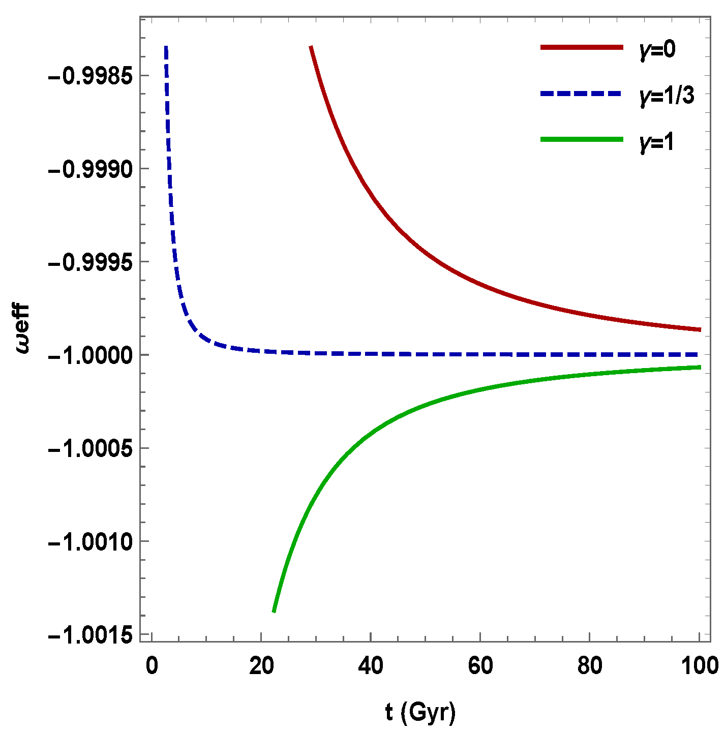
• From the behavior of the EoS parameter, it is observed that ${\omega }_{eff}$ lies in the quintessence region for $\gamma =0$; for $\gamma =1/3$, the ${\omega }_{eff}$ approaches the $\mathsf{\Lambda }$CDM point; for $\gamma =1$, the model lies in a phantom region (see Figure 3).
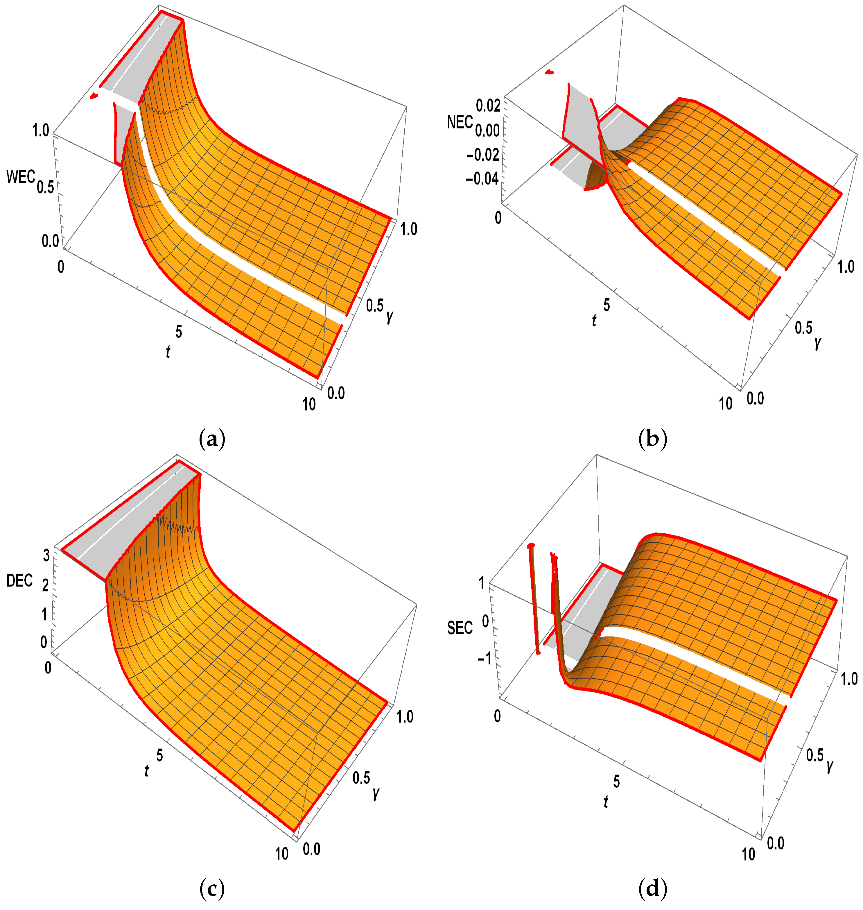
• All energy conditions, with the exception of the SEC, are satisfied in both the early- and late-time stages, according to our analysis of the energy conditions for all three types of models $\gamma =0,1/3,1$. According to recent results for the accelerating Universe, the SECs must be violated on a cosmological scale (see Figure 4a–d).
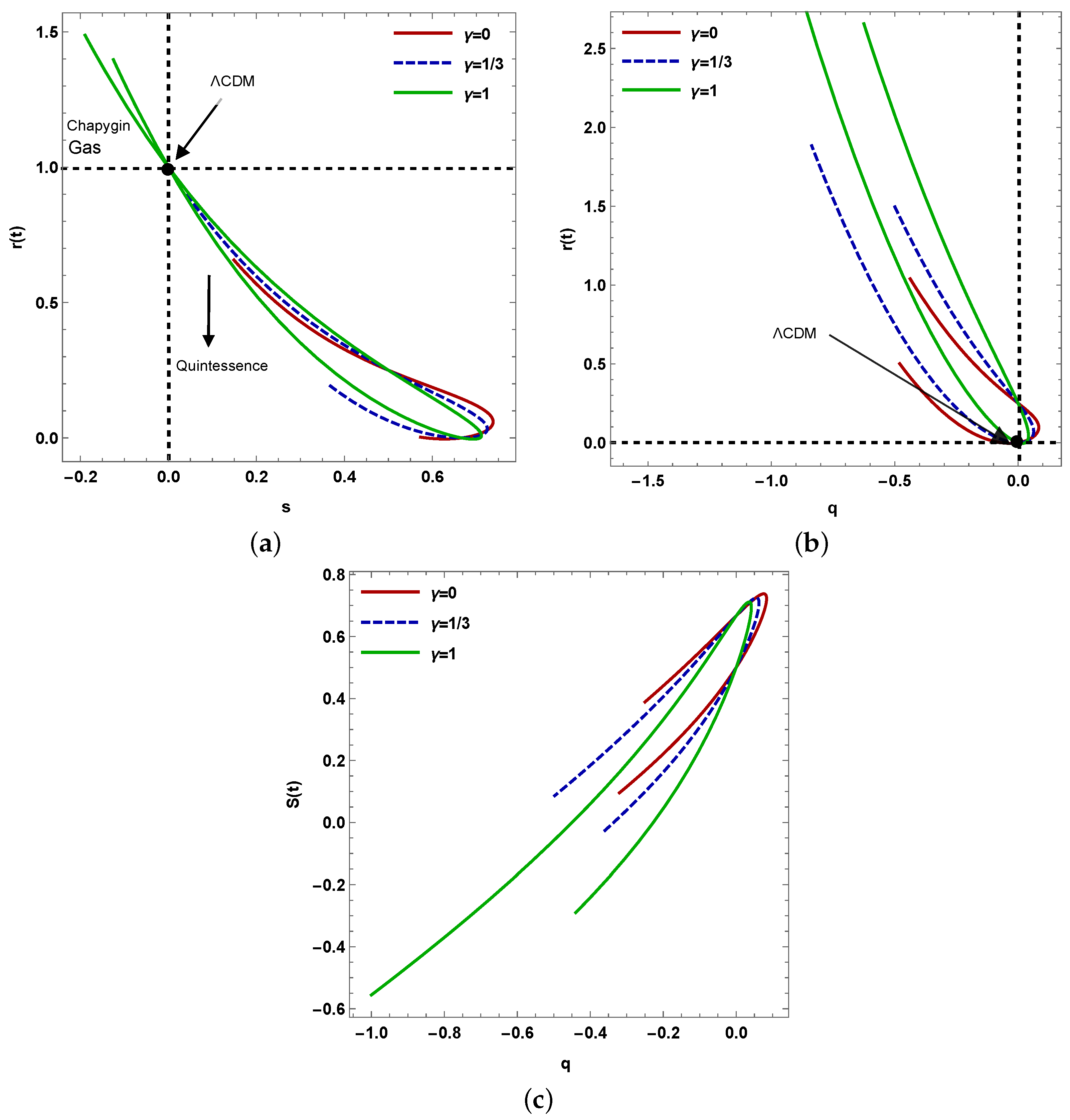
• In the case of $\kappa (R,t)$ gravity theory, the statefinders play a significant role. Our findings are described in Figure 6a–c, demonstrating that $(r,s)$, $(r,q)$, and $(s,q)$ are good diagnostics of dark energy. Figure 5a depicts that the model converges to the fixed point $(r=1,s=0)$ ($\mathsf{\Lambda }$CDM), but also traverses the Chaplygin gas and quintessence regions (see, Figure 5a–c).
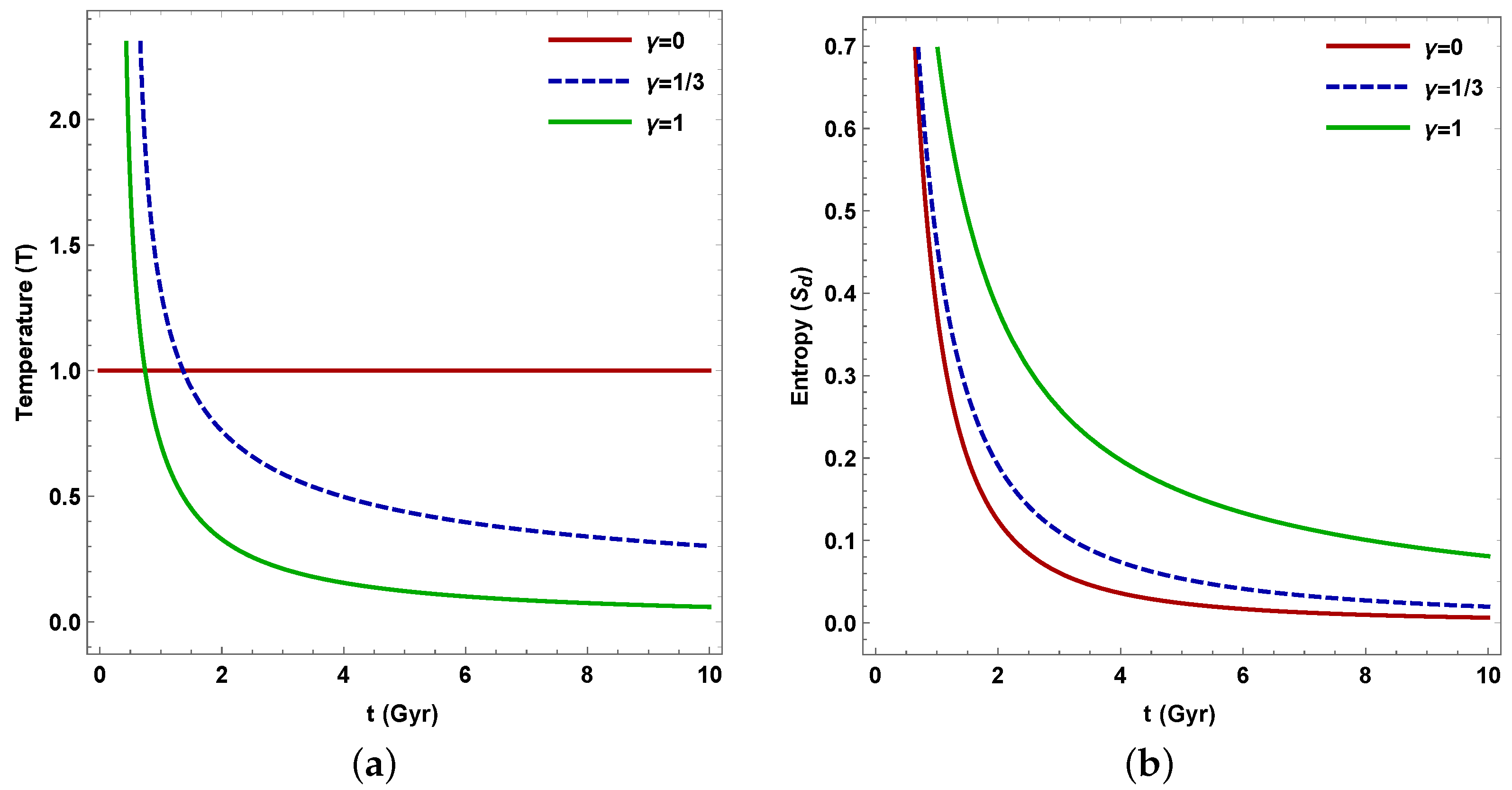
• From a thermodynamic perspective, we observed that the temperature of our model is decreasing with time and that the entropy density is positive (see, Figure 6a,b).
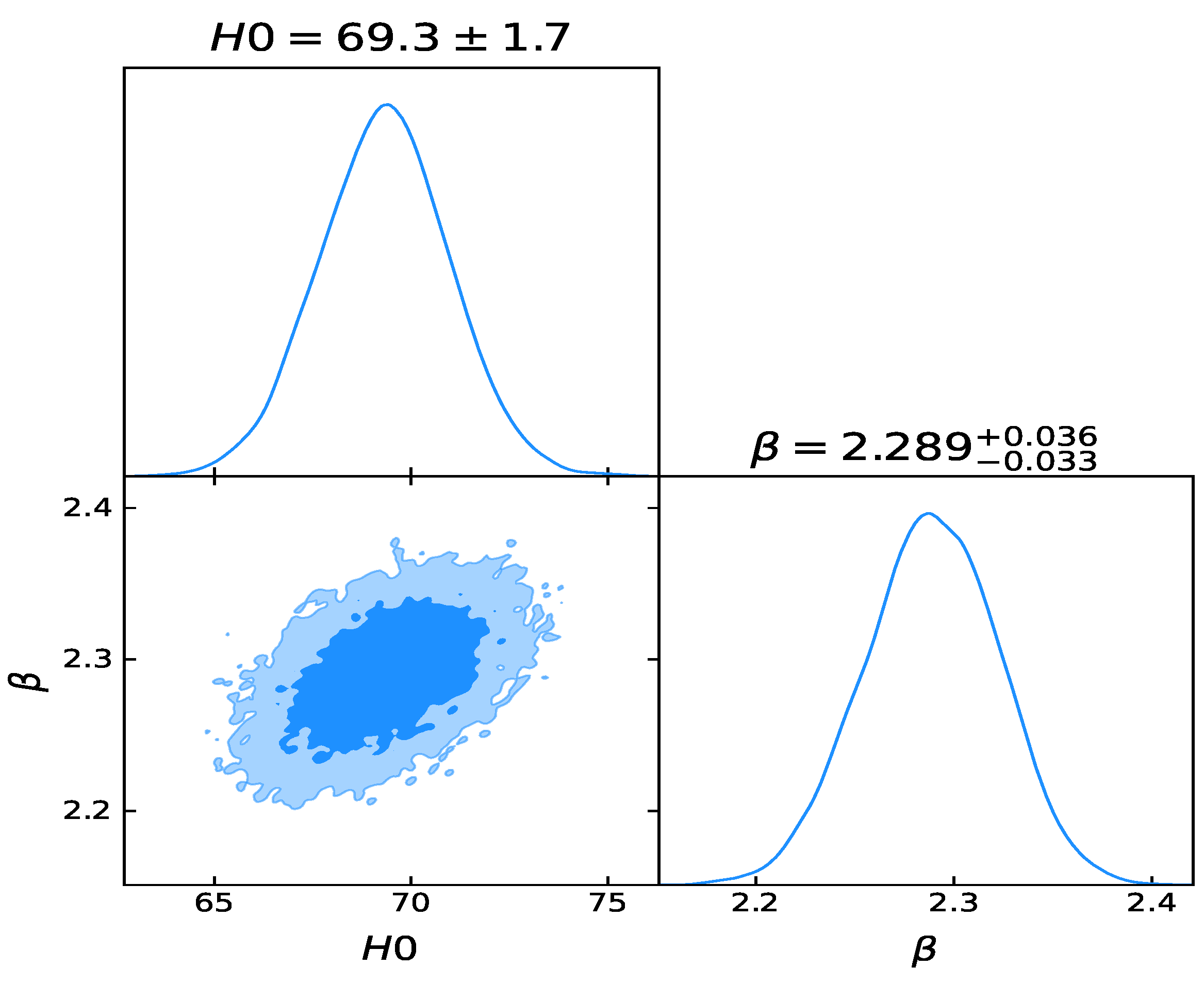
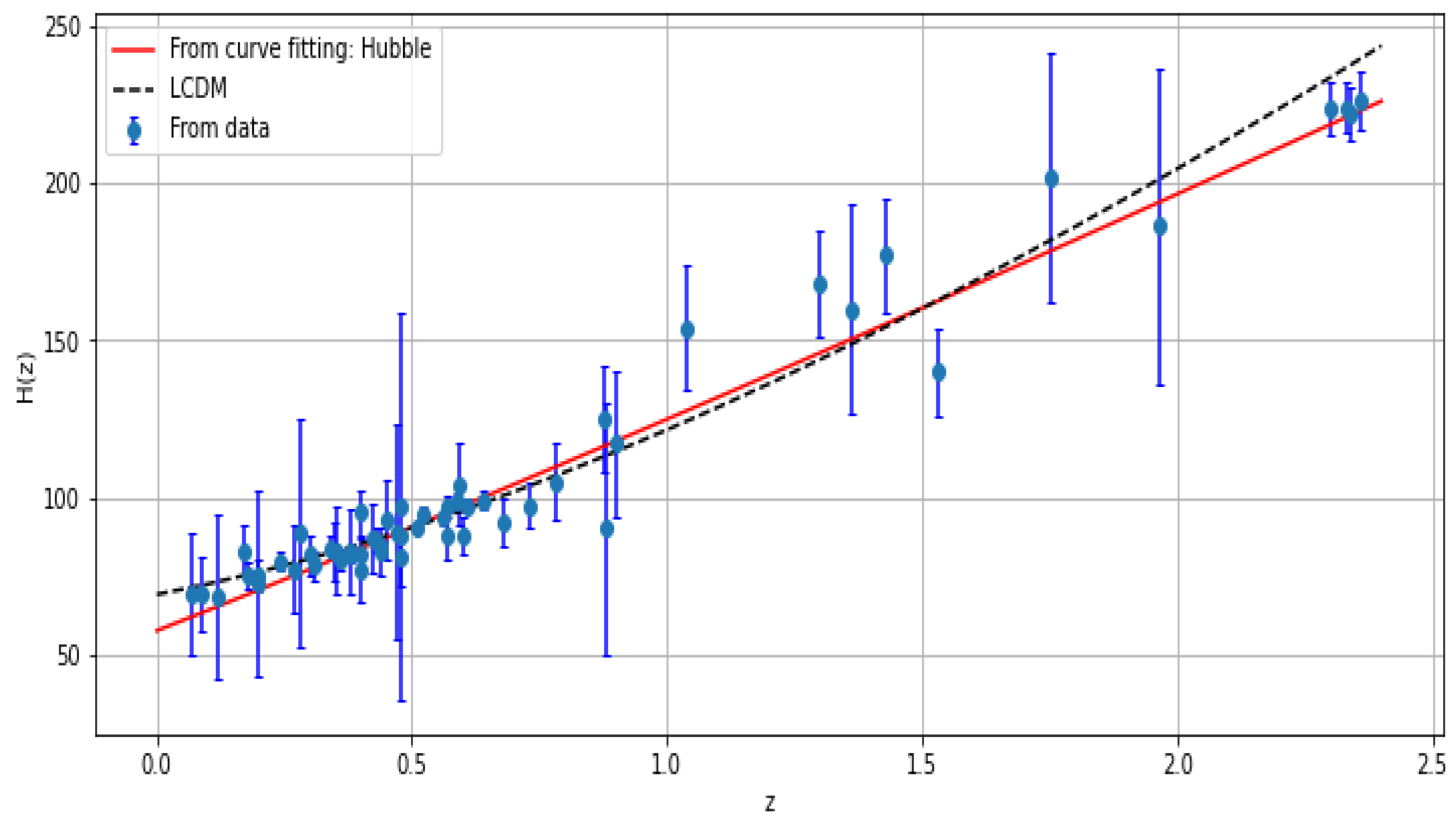
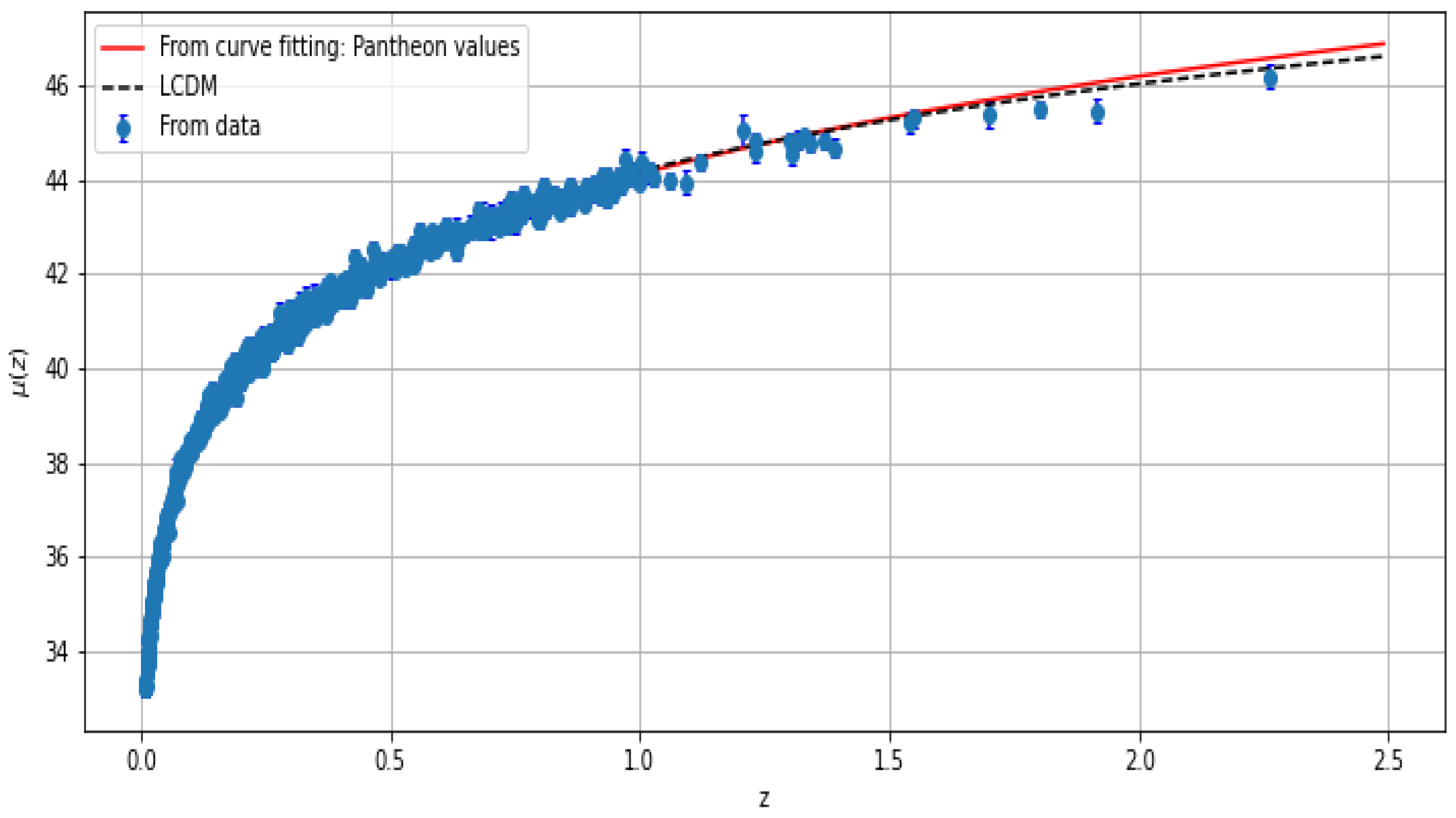
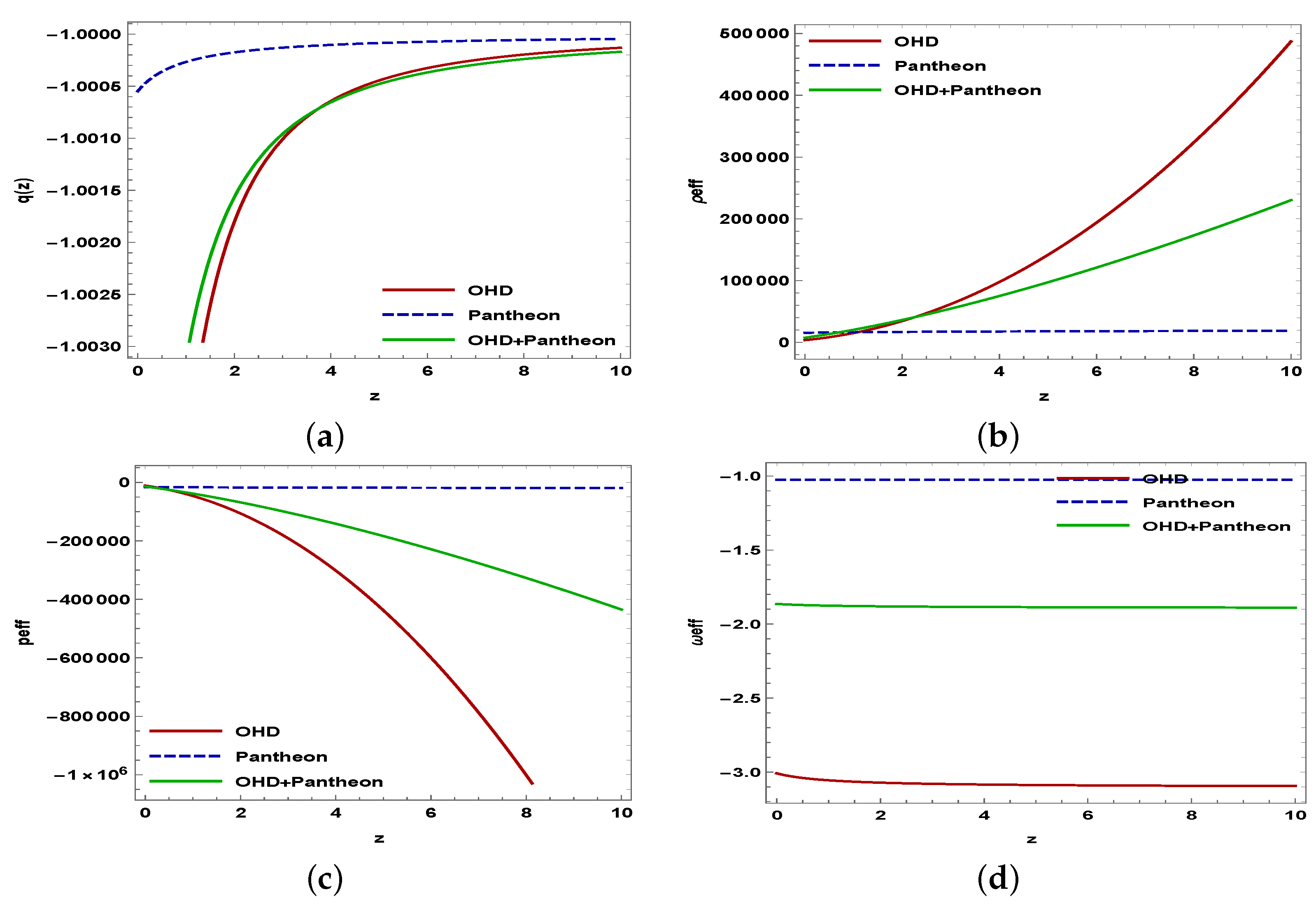
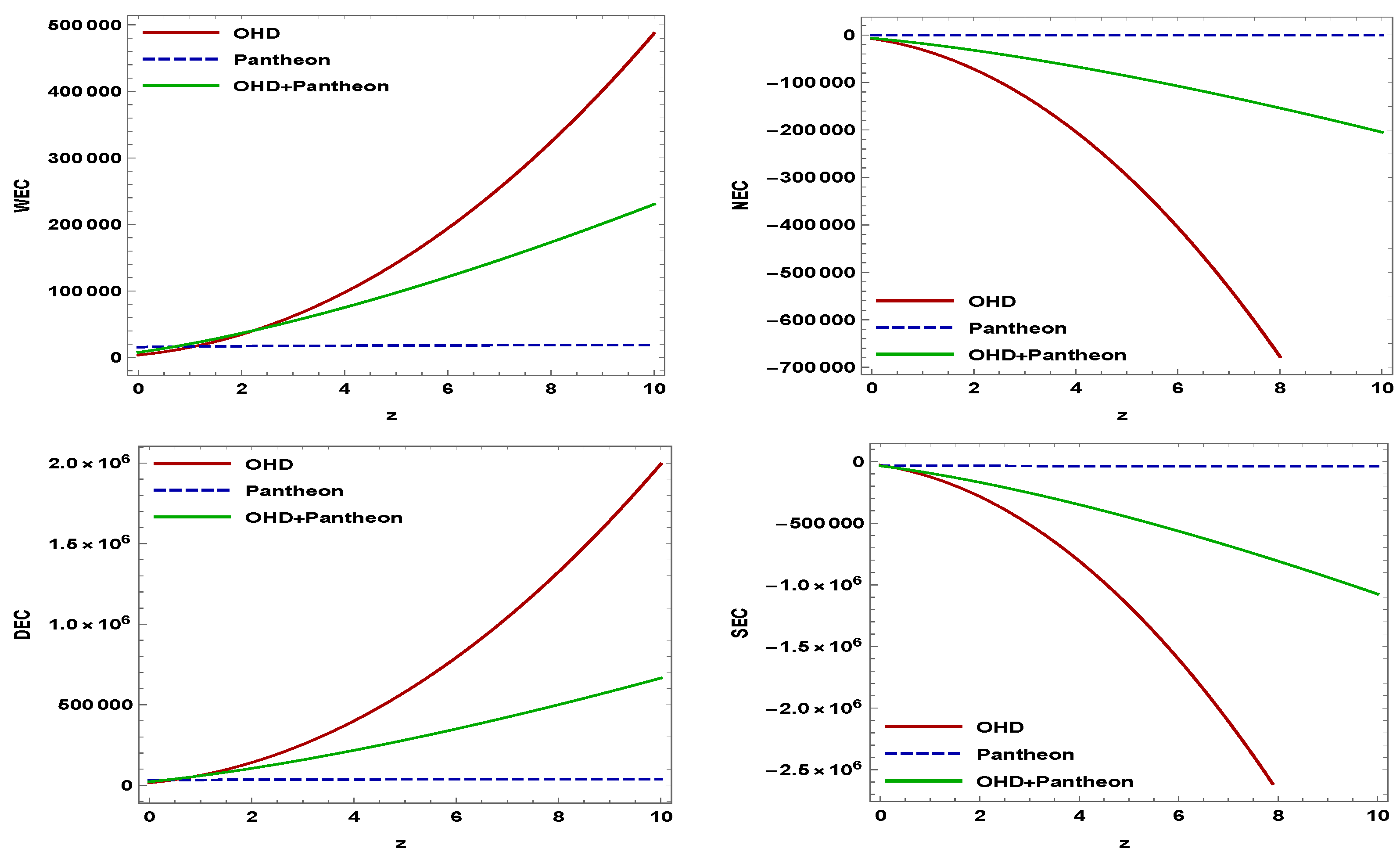
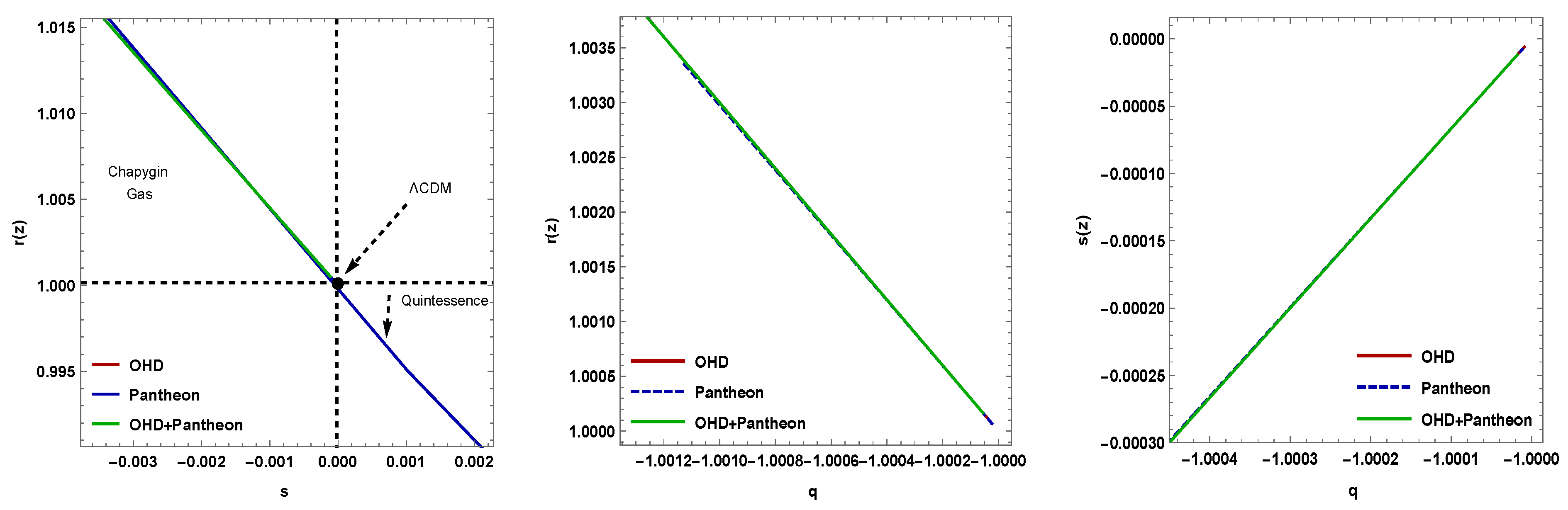
• In Figure 7, the 2D contour plots show the best-fit values of $H_0$ and $\beta$ from the EMCEE codes for the OHD, Pantheon, and OHD+Pantheon datasets. Similarly, Figure 8 and Figure 9 for H(z) and $\mu \left(z\right)$ show how well our model fits the data and how it compares to the $\mathsf{\Lambda }$CDM model. They also show the error bars for the 57 points and 1048 points of the Hubble datasets and Pantheon datasets that were used. We can see the our model is accelerated (see Figure 10a) and the behavior of the density and pressure are the standard ones (see Figure 10b,c). The EoS parameter lies in the phantom region, which indicates an accelerating phase (see Figure 10d). The plots of the energy conditions in Figure 11 show that the WECs and DECs are met, but the NECs and SECs are not. The SECs’ discrepancy correlates with the acceleration of cosmic expansion. The nature of the dark energy concept is seen in Figure 12. The derived model is now in the quintessence area and shows the $\mathsf{\Lambda }$CDM point in ($r,s$), but it will deviate significantly from the $\mathsf{\Lambda }$CDM model in the future ($r-q$).

As a consequence, this research will contribute to a better understanding of the behavior and development of the cosmos under $\kappa$ gravity.

References

1. Riess, A.; Filippenko, A.V.; Challis, P.; Clocchiattia, A.; Diercks, A.; Garnavich, P.M.; Gilliland, R.L.; Hogan, C.J.; Jha, S.; Kirshner, R.P.; et al. Observational Evidence from Supernovae for an Accelerating Universe and a Cosmological Constant. Astron. J. 1998, 116, 1009–1038. [Google Scholar] [CrossRef] [Green Version]
2. Perlmutter, S.; Aldering, G.; Goldhaber, G.; Knop, R.A.; Nugent, P.; Castro, P.G.; Deustua, S.; Fabbro, S.; Goobar, A.; Groom, D.E.; et al. Measurements of Ω and Λ from 42 High-redshift Supernovae. Astrophys. J. 1999, 517, 565–586. [Google Scholar] [CrossRef]
3. Astier, P.; Guy, J.; Regnault, N.; Pain, R.; Aubourg, E.; Balam, D.; Basa, S.; Carlberg, R.G.; Fabbro, S.; Fouchez, D.; et al. The Supernova Legacy Survey: Measurement of Ωm, ΩΛ and ω from the First Year Data Set. Astron. Astrophys. 2006, 447, 31–48. [Google Scholar] [CrossRef] [Green Version]
4. Zel’dovich, Y.B. The Cosmological Constant and the Theory of Elementary Particles. Sov. Phys. Usp. 1968, 11, 381–393. [Google Scholar] [CrossRef]
5. Turner, M.S.; Huterer, D.S. Cosmic Acceleration, Dark Energy, and Fundamental Physics. J. Phys. Soc. Jpn. 2007, 76, 111015. [Google Scholar] [CrossRef] [Green Version]
6. Knop, R.A.; Aldering, G.; Amanullah, R.; Astier, P.; Blanc, G.; Burns, M.S.; Conley, A.; Deustua, S.E.; Doi, M.; Ellis, R.; et al. New Constraints on ΩM, ΩΛ, and ω from an Independent Set of Eleven High-Redshift Supernovae Observed with HST. Astrophys. J. 2003, 598, 102–137. [Google Scholar] [CrossRef] [Green Version]
7. Capozziello, S.; Vignolo, S. On the Well-formulation of the Initial Value Problem of Metric-affine f (R)-Gravity. Int. J. Geom. Methods Mod. Phys. 2009, 6, 985. [Google Scholar] [CrossRef]
8. Nojiri, S.; Odintsov, S.D. Unified Cosmic History in Modified Gravity: From f (R) theory to Lorentz noninvariant models. Phys. Rep. 2011, 505, 59. [Google Scholar] [CrossRef] [Green Version]
9. Cai, Y.F.; Capozziello, S.; De Laurentis, M.; Saridakis, E.N. f (T) Teleparallel Gravity and Cosmology. Rep. Prog. Phys. 2016, 79, 106901. [Google Scholar] [CrossRef] [Green Version]
10. Pradhan, A.; Dixit, A.; Varshney, G. LRS Bianchi type-I Cosmological Models with Periodic Time Varying Deceleration Parameter in f (R, T) Gravity. Int. J. Mod. Phys. A 2022, 37, 2250121. [Google Scholar] [CrossRef]
11. Zubair, M.; Zeeshan, M.; Hasan, S.S.; Oikonomou, V.K. Impact of Collisional Matter on the Late-time Dynamics of f (R, T) gravity. Symmetry 2018, 10, 463. [Google Scholar] [CrossRef] [Green Version]
12. Sharma, U.K.; Kumar, M.; Varshney, G. Scalar Field Models of Barrow Holographic Dark Energy in f (R, T) Gravity. Universe 2022, 8, 642. [Google Scholar] [CrossRef]
13. Bamba, K.; Odintsov, S.D.; Sebastiani, L.; Zerbini, S. Finite-time Future Singularities in Modified Gauss-Bonnet and F(R, G) Gravity and Singularity Avoidance. Eur. Phys. J. C 2010, 67, 295. [Google Scholar] [CrossRef]
14. Tangphati, T.; Pradhan, A.; Errehymy, A.; Banerjee, A. Quark Stars in the Einstein-Gauss-Bonnet theory: A New Branch of Stellar Configurations. Ann. Phys. 2021, 430, 168498. [Google Scholar] [CrossRef]
15. Naicker, S.; Maharaj, S.D.; Brassel, B.P. Isotropic perfect fluids in modified gravity. Universe 2023, 9, 47. [Google Scholar] [CrossRef]
16. Shekh, S.H.; Moraes, P.H.R.S.; Sahoo, P.K. Physical Acceptability of the Renyi, Tsallis and Sharma-Mittal Holographic Dark Energy Models in the f (T, B) Gravity under Hubble’s Cutoff. Universe 2022, 7, 67. [Google Scholar] [CrossRef]
17. Dixit, A.; Pradhan, A. Bulk viscous FLRW model with Observational Constraints in f (T, B) Gravity. Universe 2022, 8, 650. [Google Scholar] [CrossRef]
18. Godani, N.; Samanta, G.C. FRW Cosmology in f (Q, T) Gravity. Int. J. Geom. Methods Mod. Phys. 2021, 18, 2150134. [Google Scholar] [CrossRef]
19. Pradhan, A.; Dixit, A. The Models of Transit Cosmology along with Observational Constriction in f (Q, T) Gravity. Int. J. Geom. Methods Mod. Phys. 2021, 18, 2150159. [Google Scholar] [CrossRef]
20. Sharma, U.K.; Shweta; Mishra, A.K. Traversable wormhole solutions with non-exotic fluid in framework of f (Q) gravity. Int. J. Geom. Methods Mod. Phys. 2022, 19, 2250019. [Google Scholar] [CrossRef]
21. Pradhan, A.; Dixit, A.; Maurya, D.C. Quintessence Behaviour of an Anisotropic Bulk Viscous Cosmological Model in Modified f(Q)-gravity. Symmetry 2022, 14, 2630. [Google Scholar] [CrossRef]
22. Shekh, S.H.; Myrzakulov, N.; Pradhan, A.; Mussatayera, A. Observational constraints on F(T, TG) gravity with Hubble parametrization. Symmetry 2023, 15, 321. [Google Scholar] [CrossRef]
23. Linder, E.V. Einstein’s other Gravity and the Acceleration of the Universe. Phys. Rev. D 2010, 81, 127301. [Google Scholar] [CrossRef] [Green Version]
24. Capozziello, S.; Carloni, S.; Troisi, A. Quintessence without Scalar Fields. Recent Res. Dev. Astron. Astrophys. 2003, 1, 625. [Google Scholar]
25. Harko, T.; Lobo, F.S.N.; Nojiri, S.; Odintsov, S.D. f (R, T) Gravity. Phys. Rev. D 2011, 84, 024020. [Google Scholar] [CrossRef] [Green Version]
26. Nojiri, S.; Odintsov, S.D.; Oikonomou, V.K. Modified Gravity Theories on a Nutshell: Inflation, Bounce and Late-time Evolution. Phys. Rep. 2017, 692, 1–104. [Google Scholar] [CrossRef] [Green Version]
27. Teruel, G.R.P. κ(R, T) Gravity. Europhys. J. C 2018, 78, 660. [Google Scholar]
28. Ahmed, N.; Pradhan, A. Probing Cosmic Acceleration in κ(R, T) Gravity. Indian J. Phys. 2022, 96, 301–307. [Google Scholar] [CrossRef]
29. Nojiri, S.; Odintsov, S.D. Modified f (R) Gravity consistent with Realistic Cosmology: From a Matter Dominated Epoch to a Dark Energy Universe. Phys. Rev. D 2006, 74, 086005. [Google Scholar] [CrossRef] [Green Version]
30. Rastall, P. Generalization of the Einstein Theory. Phys. Rev. D 1972, 6, 3357. [Google Scholar] [CrossRef]
31. Einstein, A. Die Feldgleichungen der Gravitation; Sitzungsberichte der PreussischenAkademie der Wissenschaften: Berlin, Germany, 1915; pp. 844–847. [Google Scholar]
32. Renn, J.; Schemmel, M. The Genesis of General Relativity; Springer: Berlin/Heidelberg, Germany, 2007. [Google Scholar]
33. Hilbert, D. Die Grundlagen der Physik. Konigl. Gesell. d. Wiss. Göttingen. Nachr. Math.-Phys. Kl. 1915, 1915, 395–407. [Google Scholar]
34. Maxwell, J.C. On physical lines of force. Philos. Mag. 1861, 90, 11–23. [Google Scholar] [CrossRef]
35. Bennett, C.L.; Halpern, M.; Hinshaw, G.; Jarosik, N.; Kogut, A.; Limon, M.; Meyer, S.S.; Page, L.; Spergel, D.N.; Tucker, G.S.; et al. First year Wilkinson Microwave Anisotropy Probe (WMAP) Observations: Preliminary Maps and Basic Results. Astrophys. J. Suppl. 2003, 148, 1. [Google Scholar] [CrossRef] [Green Version]
36. Beck, C. Axiomatic approach to the cosmological constant. Phys. A 2009, 388, 3384. [Google Scholar] [CrossRef] [Green Version]
37. We, H.; Zou, X.B.; Li, H.Y.; Xue, D.Z. Cosmological constant, fine structure constant and beyond. Eur. Phys. J. C 2017, 77, 14. [Google Scholar] [CrossRef] [Green Version]
38. Wang, P.; Meng, X.H. Can vacuum decay in our Universe? Class. Quantum Gravity 2005, 22, 283. [Google Scholar] [CrossRef] [Green Version]
39. Overduin, J.M.; Cooperstock, F.I. Evolution of the scale factor with a variable cosmological term. Phys. Rev. D 1998, 58, 043506. [Google Scholar] [CrossRef] [Green Version]
40. Overduin, J.M.; Wesson, P.S. Dark Matter and Background Light. Phys. Rep. 2004, 402, 267. [Google Scholar] [CrossRef] [Green Version]
41. Carvalho, J.C.; Lima, J.A.S.; Waga, I. Cosmological consequences of a time-dependent Λ term. Phys. Rev. D 1992, 46, 2404. [Google Scholar] [CrossRef]
42. Dixit, A.; Pradhan, A.; Chaubey, R. Cosmological Scenario in κ(R, T) Gravity. Int. J. Geom. Methods Mod. Phys. 2022, 19, 2250013. [Google Scholar] [CrossRef]
43. Wang, B.; Gong, Y.; Abdalla, E. Thermodynamics of an Accelerated Expanding Universe. Phys. Rev. D 2006, 74, 083520. [Google Scholar] [CrossRef] [Green Version]
44. Ade, P.A.R.; Aghanim, N.; Arnaud, M.; Ashdown, M.; Aumont, J.; Baccigalupi, C.; Banday, A.J.; Barreiro, R.B.; Bartolo, N.; Battaner, P.; et al. Planck 2015 results XIV. Dark energy and modified gravity. Astron. Astrophys. 2016, 594, A14. [Google Scholar]
45. Hinshaw, G.F.; Larson, D.; Komatsu, E.; Spergel, D.N.; Bennett, C.L.; Dunkley, J.; Nolta, M.R.; Halpern, M.; Hill, R.S.; Odegard, N.; et al. Nine-year Wilkinson Microwave Anisotropy Probe (WMAP) Observations: Cosmological Parameter Results. Astrophys. J. Suppl. Ser. 2013, 208, 19. [Google Scholar] [CrossRef] [Green Version]
46. Komatsu, E.J.; Dunkley, M.R.; Nolta, C.L.; Bennett, B.; Gold, G.; Hinshaw, N.; Jarosik, D.; Larson, M.; Limon, L.; Page, D.; et al. WMAP, Five-year Wilkinson Microwave Anisotropy Probe Observations: Cosmological Interpretation. Astrophys. J. Suppl. 2009, 180, 330–376. [Google Scholar] [CrossRef] [Green Version]
47. Feng, B.; Wang, X.L.; Zhang, X.M. Dark energy Constraints from the Cosmic age and Supernova. Phys. Lett. B 2005, 607, 35. [Google Scholar] [CrossRef]
48. Pradhan, A.; Zia, R.; Singh, R.P. Viscous Fluid Cosmology with Time Dependent q and Λ-term in Bianchi Type-I Space-time and late time acceleration. Indian J. Phys. 2013, 87, 1157–1167. [Google Scholar] [CrossRef]
49. Capozziello, S.; Nojiri, S.I.; Odintsov, S.D. The role of Energy Conditions in f (R) Cosmology. Phys. Lett. B 2018, 781, 99. [Google Scholar] [CrossRef]
50. Sharma, U.K.; Dubey, V.C. Statefinder Diagnostic for the Renyi Holographic Dark Energy. New Astron. 2020, 80, 101419. [Google Scholar] [CrossRef]
51. Sahni, V.; Saini, T.D.; Starobinsky, A.A.; Alam, U. Statefinder-A new geometrical diagnostic of dark energy. JETP Lett. 2003, 77, 201. [Google Scholar] [CrossRef]
52. Alam, U.; Sahni, V.; Saini, T.D.; Starobinsky, A.A. Exploring the Expanding Universe and Dark Energy using the Statefinder Diagnostic. Mon. Not. R. Astron. Soc. 2003, 344, 1057. [Google Scholar] [CrossRef]
53. Sami, M.; Shahalam, M.; Skugoreva, M.; Toporensky, A. Cosmological Dynamics of a Nonminimally Coupled Scalar Field System and its Late Time Cosmic Relevance. Phys. Rev. D 2012, 86, 103532. [Google Scholar] [CrossRef] [Green Version]
54. Tu, F.Q.; Chen, Y.X.; Huang, Q.H. Thermodynamics in the Universe described by the emergence of Space and the Energy Balance Relation. Entropy 2019, 21, 167. [Google Scholar] [CrossRef] [PubMed] [Green Version]
55. Chen, Y.; Kumar, S.; Ratra, B. Determining the Hubble constant from Hubble parameter measurements. Astrophys. J. 2017, 835, 86. [Google Scholar] [CrossRef] [Green Version]
56. Ade, P.A.; Aghanim, N.; Armitage-Caplan, C.; Arnaud, M.; Ashdown, M.; Atrio-Barandela, F.; Aumont, J.; Baccigalupi, C.; Banday, A.J.; Barreiro, R.B.; et al. Planck 2013 results XVI Cosmological parameters. Astron. Astrophys. 2014, 571, A16. [Google Scholar]
57. Suzuki, N.; Rubin, D.; Lidman, C.; Aldering, G.; Amanullah, R.; Barbary, K.; Barrientos, L.F.; Botyanszki, J.; Brodwin, M.; Connolly, N.; et al. The Hubble Space Telescope cluster supernova survey. Improving the dark-energy constraints above z > 1 and building an early-type-hosted supernova sample. Astrophy. J. 2012, 746, 85. [Google Scholar] [CrossRef] [Green Version]
Figure 1. The plot of deceleration parameter q ( t ) versus time t for γ = 0 , 1 / 3 and 1 . Here, β = 1.5 , c 1 = 0.5 .
Symmetry 15 00549 g001
Figure 2. (a) The plot of effective energy density ρ e f f versus time t for γ = 0 , 1 / 3 and 1 . (b) The plot of effective pressure p e f f versus time t for γ = 0 , 1 / 3 and 1 . Here, β = 1.5 , c 1 = 0.5 , and k 1 = 1 .
Symmetry 15 00549 g002
Figure 3. The plot of EoS parameter versus time t for γ = 0 , 1 / 3 and 1 . Here, β = 1.5 , c 1 = 0.5 , k 1 = 1 .
Symmetry 15 00549 g003
Figure 4. The plots of energy conditions (a) WECs, (b) NECs, (c) DECs, and (d) DECs versus time t and γ respectively. Here, β = 1.5 , c 1 = 0.5 , and k 1 = 1 . The scale of time t is taken in Gyr.
Symmetry 15 00549 g004
Figure 5. (a) The plot of ( r s ) . (b) The plot of ( r q ) . (c) The plot of ( s q ) . Here, β = 1.5 , c 1 = 0.5 , and k 1 = 1 .
Symmetry 15 00549 g005
Figure 6. (a) Evolution of thermodynamical temperature T in the κ ( R , T ) gravity model. (b) Evolution of thermodynamical entropy density S d in the κ ( R , T ) gravity model. Here, β = 1.5 , c 1 = 0.5 , and k 1 = 1 .
Symmetry 15 00549 g006
Figure 7. The 1 σ and 2 σ likelihood contours for the model parameters with H ( z ) + P a n t h e o n data.
Symmetry 15 00549 g007
Figure 8. The figure depicts the error bar plot of the 57 OHD points with the fitting of Hubble function H ( z ) versus redshift. This plot is compared to the conventional Λ CDM.
Symmetry 15 00549 g008
Figure 9. The error bar plot of the 1048 points of the Pantheon compilation SNe Ia datasets is shown in the image, along with the fitting of function μ ( z ) and redshift z for comparison with the conventional Λ CDM model.
Symmetry 15 00549 g009
Figure 10. (a) Behavior of deceleration parameter versus redshift. (b) Behavior of effective density versus redshift. (c) Behavior of effective pressure versus redshift. (d) Behavior of EoS parameter versus redshift.
Symmetry 15 00549 g010
Figure 11. Behavior of all types of energy conditions against redshift for various observational data.
Symmetry 15 00549 g011
Figure 12. Behavior of statefinder trajectories ( r s ) , ( r q ) , and ( s q ) .
Symmetry 15 00549 g012