Article

Analysis of the Competition System Using Parameterized Fractional Differential Equations: Application to Real Data

by
Mahmoud H. DarAssi
1,
Muhammad Altaf Khan
2,3,
Fatmawati
3,* and
Marei Saeed Alqarni
4
1
Department of Basic Sciences, Princess Sumaya University for Technology, Amman 11941, Jordan
2
Faculty of Natural and Agricultural Sciences, University of the Free State, Bloemfontein 9301, South Africa
3
Department of Mathematics, Faculty of Science and Technology, Universitas Airlangga, Surabaya 60115, Indonesia
4
Department of Mathematics, College of Science, King Khalid University, Abha 61413, Saudi Arabia
*
Author to whom correspondence should be addressed.
Symmetry 2023, 15(2), 542; https://doi.org/10.3390/sym15020542
Submission received: 3 January 2023 / Revised: 18 January 2023 / Accepted: 8 February 2023 / Published: 17 February 2023
(This article belongs to the Special Issue Mathematical Modeling of the Infectious Diseases and Their Controls)

Abstract

:
Natural symmetries exist in several processes of chemistry, physics, and biology. Symmetries possess interesting dynamical characteristics that cannot be seen in non-symmetric systems. The present paper investigates the competition between two banking systems, rural and commercial, in Indonesia, in parameterized fractional order Caputo derivative. A novel numerical method is used to discretize the competition system using the real data of rural and commercial banks in Indonesia for the period 2004–2014. The new scheme is more suitable and reliable for data fitting results and has good accuracy. The integer model is formulated in Caputo derivative and their stability results are presented. With the available parameters, the data for the model is analyzed using various scenarios. We shall compare the result with the previous method used in the literature and show that the present method is better than the previous method in the literature. It is shown that fractional order α and the parameter ρ involved in the numerical scheme provide excellent fitting.

1. Introduction

Many biological, chemical, and physical systems exhibit natural symmetry. Therefore, including these symmetries in the differential equations used to explain the systems is a sensible modeling assumption. Understanding the structure of differential equation solutions that adhere to the restrictions set by the symmetry group is essential to studying differential equations with symmetry, also known as equivalent differential equations. Symmetries can be temporal or geographical.
Mathematical models are useful when studying the practical problems arising in science and engineering and for determining the long-time behavior. The applications of the mathematical models to physics, mathematics, and other areas of science and engineering have already been documented in literature while in social sciences it is also been applied, and very interesting results have been obtained. Besides this, in financial areas, the application of mathematical models is getting more attention day by day. The banks, whether they are commercial or rural, are crucial in the development of the country’s economic growth. Strong banking practices and their maximum advantages to the populace are essential to the development of a nation [1]. It should be highlighted that the banking sector can be either conventional or Islamic, or it can be both. The banks that adhere to Syrian law or do things traditionally are defined under Act No. 10 of 1998. The operations of commercial and rural banks in Indonesia have been examined, and it has been proven that the latter engage in more business activities than the former [2,3]. Additionally, there are more commercial banks in Indonesia than rural ones, however, both banks offer the same products [4]. Commercial banks are more numerous than rural banks, but rural banks are still enhancing their business operations to draw in more clients. Rural banks may face competition from commercial banks as a result of enhancements to their business products.
The rural banks in Indonesia may face intense competition if they keep working to improve their products. The Lotka–Volterra system of evolutionary differential equations can be used to study this competition efficiently [5]. To analyze the competition’s numerous genuine word problems, the researchers used the Lotka–Volterra equations; for more information; see Refs. [6,7,8,9,10,11,12,13]. For instance, the competition system is used to examine the mobile company data of Korean companies [6]. Additional applications include modeling technology replacement (see Ref. [7]), and modeling of policy and its effects on the Korean stock market, and competition between banking sectors (see Refs. [8,9,10,11]). Additionally, some recent research on this topic can be found in Refs. [12,13,14,15].
It is important to note that the Lotka–Volterra system was employed in the aforementioned study to determine the dynamics of various problems with integer order, except for Refs. [12,13,14,15]. The application of the competition system to marine phage population dynamics has been considered in Ref. [16]. The Lotka–Volterra system applications to a three-level laser and their dynamics have been considered in Ref. [17]. The competition and sales of two competing retail formats using the Lotka–Volterra system have been analyzed in Ref. [18]. The seasonal succession using the Lokta–Volteerra model has been discussed by the authors in Ref. [19]. In Ref. [20], the authors considered the competition mixture and their complex fitness using the competition system.
In recent years, it has become clear that fractional calculus is crucial to the dynamic modeling of these kinds of real-world issues. Memory and hereditary properties are thought to be one of the causes. Real-world problems frequently have nonlinear models with crossover behavior, which makes it challenging to address them precisely. Such applications of the fractional order models with real-life problems may be shown in Refs. [21,22,23,24,25,26,27]. Recently, the authors in Ref. [28] considered a tumor disease study using fractional differential equations. A prey-predator system using fractional order derivative has been studied in Ref. [29]. The fractional order model for HIV of cell-to-cell dynamics has been analyzed in Ref. [30]. The discrete food chain model using fractional discrete derivative has been discussed in Ref. [31]. The important application of the fractional models is to fit well with the real data because there is more choice for the fractional order parameters, such as variable, or of constant order. Such remarkable benefits make it more powerful than the integer order systems; see Refs. [14,15,21]. For the fractional calculus used recently in literature when dealing the financial systems, see Refs. [32,33,34].
This research aims to investigate the banking data competition between two Indonesian banks using actual statistical data and a parameterized fractional order model. The Caputo derivative is the fractional derivative taken into account in this work. We employ the recently established numerical technique, utilizing the parameterized method for the numerical solution of the fractional model; see Ref. [35]. The method has been tested for various linear and nonlinear problems and found suitable fractional differential equations. Compared to existing techniques for fractional models that are accessible in the literature, this new method is more accurate and reasonable. We shall present the comparison of the present method with the FDE12 method. The FDE method was used for the fractional differential equation in the Caputo case. We shall see that the present method is better than FDE12 when considering the numerical value of ρ . The suggested method will demonstrate how the data fits nicely when the parameterized order and particular fractional orders are taken into account. The remaining findings in this research are as follows: Section 2 displays the model along with its descriptions. Section 3 displays the integral and related definitions. Section 4 illustrates the numerical results of the system with the new scheme that is designed for the fractional differential equation in the power law kernel by providing the algorithm. Section 5 presents a discussion of the results. Section 6 presents the achievements of the results of this work.

2. Basics of Fractional Operators

The development in fractional calculus is still underway with new discoveries in the form of analytical and numerical shapes. This section highlights the definitions that will be considered in this work, which are obtained from Ref. [35]. Let g be differentiable within [ 0 , T ] then
0 F c D t α g ( t ) = 1 Γ ( α ) 0 t g ( β ) K ( t β ) d β
where K ( t ) = t α ,
θ ( α ) = 1 Γ ( α ) or 1 1 α , 0 < α 1 .
The Caputo derivative is given by [36],
0 C D t α g ( t ) = 1 Γ ( n α ) 0 t ( t β ) n α 1 g n ( β ) d β .
The integral to (3) is given by
0 C I t α ( g ( t ) ) = 1 Γ ( α ) 0 t g ( β ) ( t β ) α 1 d β .

3. Mathematical Model

Mathematical models are useful to study the competition among species. Competition is not only among species, but also among other social sciences activities such as bank competitions or competition among different companies of their product. We shall consider the Indonesian banks that are rural and commercials using the well-known Lotka–Volterra system. We shall denote the profit of the commercial banks by C ( t ) at any time t while the rural banks are given by R ( t ) . It is assumed that the banks have maximum profit and their limited funds behave as logistical growths. Thus, we can write the ordinary differential equation as
d C d t = g 1 C 1 C L 1 q 1 C R ,
d R d t = g 2 R 1 R L 2 q 2 C R ,
where the the initial conditions are C ( 0 ) = C 0 0 , and R ( 0 ) = R 0 0 . The parameter g 1 defines the growth rate of the commercial bank while g 2 stands for the growth rate of the rural banks. The parameter L 1 is the maximum profit gained by the commercial banks while L 2 is for the rural banks. q 1 and q 2 are the competition factors of commercial and rural banks. The parameters used in the system (5) are clearly positive.

3.1. Fractional Order Model

The model given by (5) is formulated in fractional differential equation using the Caputo definitions, and it is given by:
0 C D t α C ( t ) = g 1 C 1 C L 1 q 1 C R ,
0 C D t α R ( t ) = g 2 R 1 R L 2 q 2 C R ,
where α is defined to be the fractional order in the sense of Caputo derivative while the initial conditions are C ( 0 ) = C 0 0 and R ( 0 ) = R 0 0 .

3.2. Existence and Uniqueness

First, we shall write the fractional order system (6) in the form below:
0 C D t α C ( t ) = h 1 ( C , R , t ) ,
0 C D t α R ( t ) = h 2 ( C , R , t ) .
Now, we define the norm,
| | C | | = sup t D | C ( ( t ) | ,
where D [ 0 , T ] . We shall assume to prove that C ( t ) and R ( t ) are bounded within [ 0 , T ] , so for any t [ 0 , T ] there exists U 1 and U 2 such that | | C | | < U 1 and | | R | | < U 2 . We need to first show h 1 and h 2 are bounded.
| h 1 ( C , R , t ) | = | g 1 C 1 C L 1 q 1 C R | , g 1 | C 1 C L 1 | + | q 1 C R | , g 1 | C | | 1 C L 1 | + | q 1 C R | , g 1 sup t [ 0 , T ] | C ( t ) | sup t [ 0 , T ] | 1 C ( t ) L 1 | + q 1 sup t [ 0 , T ] | C ( t ) | sup t [ 0 , T ] | R ( t ) | , g 1 | | C | | | 1 + | | C | | L 1 | + q 1 | | C | | | | R | | , < g 1 U 1 ( 1 + U 1 L 1 ) + q 1 U 1 U 2 , < .
Repeating the process again for the second equation of the mode (6), we shall have,
| h 2 ( C , R , t ) | = g 2 U 2 ( 1 + U 2 L 2 ) + q 2 U 1 U 2 < .
So, C ( t ) and R ( t ) are bounded, and then there exists F 1 and F 2 such that
sup t [ 0 , T ] | h 1 ( C , R , t ) | < F 1 , sup t [ 0 , T ] | h 2 ( C , R , t ) | < F 2 .
On the other hand, if for all t [ 0 , T ] , | h 1 ( C , R , t ) | < F 1 and | h 2 ( C , R , t ) | < F 2 , then | | C | | < and | | R | | < .
Proof. 
Consider that h 1 and h 2 are bounded, then
C ( t ) = C ( 0 ) + 1 Γ ( α ) 0 t h 1 ( C , R , ψ ) ( t ψ ) α 1 d ψ ,
R ( t ) = R ( 0 ) + 1 Γ ( α ) 0 t h 2 ( C , R , ψ ) ( t ψ ) α 1 d ψ .
| C ( t ) | | C ( 0 ) | + 1 Γ ( α ) | 0 t h 1 ( C , R , ψ ) ( t ψ ) α 1 d ψ | ,
| R ( t ) | | R ( 0 ) | + 1 Γ ( α ) | 0 t h 2 ( C , R , ψ ) ( t ψ ) α 1 d ψ | .
without loss of generality, we can show for C ( t ) ,
| C ( t ) | | C ( 0 ) | + 1 Γ ( α ) 0 t | h 1 ( C , R , ψ ) | ( t ψ ) α 1 d ψ , < | C ( 0 ) | + 1 Γ ( α ) 0 t sup t [ 0 , T ] | h 1 ( C , R , ψ ) | ( t ψ ) α 1 d ψ , < | C ( 0 ) | + F 1 t α Γ ( α + 1 ) < | C ( 0 ) | + F 1 T α Γ ( α + 1 ) .
Thus,
| C ( t ) | < | | C ( t ) | | < | C ( 0 ) | + F 1 T α Γ ( α + 1 ) .
We can also show,
| R ( t ) | < | | R ( t ) | | < | R ( 0 ) | + F 2 T α Γ ( α + 1 ) .
To show the unique solution of the system proposed (6), the following conditions should be met,
  • for every t [ 0 , T ] , h 1 and h 2 satisfy | h 1 ( C , R , t ) | 2 < μ 1 ( 1 + | C | 2 ) , | h 2 ( C , R , t ) | 2 < μ 2 ( 1 + | R | 2 ) ,
  • for every t [ 0 , T ] , h 1 and h 2 satisfy the Lipschitz condition | h 1 ( C 1 , R , t ) h 1 ( C 2 , R , t ) | 2 < μ ¯ 1 | C 1 C 2 | 2 , | h 2 ( C , R 1 , t ) h 2 ( C , R 2 , t ) | 2 < μ ¯ 2 | R 1 R 2 | 2 .
We shall start to prove for h 1 ,
h 1 C 1 , R , t h 1 C 2 , R , t 2 = g 1 C 1 1 C 1 L 1 q 1 C 1 R g 2 C 2 1 C 2 L 1 + q 1 C 2 R 2 , = g 1 C 1 C 2 C 1 C 1 2 L 1 C 2 2 L 1 q 1 C 1 C 2 R < 3 g 1 2 C 1 C 2 2 + 3 g 1 2 C 1 2 L 1 C 2 2 L 1 2 + 3 q 1 2 C 1 C 2 2 | R | < 3 g 1 2 + 2 g 1 2 C 1 L 1 2 + C 2 L 1 2 + q 1 2 | R | 2 C 1 C 2 2 , < 3 g 1 2 + 2 g 1 2 sup t [ 0 , T ] C 1 L 1 2 + sup t [ 0 , T ] C 2 L 1 2 + q 1 2 sup t [ 0 , T ] | R | 2 × C 1 C 2 2 , < 3 g 1 2 + 2 g 1 2 2 U 1 2 L 1 2 + q 1 2 U 2 2 C 1 C 2 2 , < μ 1 ¯ C 1 C 2 2 ,
where μ 1 ¯ = 3 g 1 2 + 2 g 1 2 2 U 1 2 L 1 2 + q 1 2 U 2 2 . On the other hand,
| h 1 ( C , R , t ) | 2 = | g 1 C ( 1 C L 1 ) q 1 C R | 2 , 3 g 1 2 | C | 2 + 3 g 1 2 C L 1 2 + 3 q 1 2 | C | 2 | R | 2 , 3 g 1 2 + 3 g 1 2 L 1 2 | C | 2 + 3 q 1 2 | R | 2 | C | 2 3 g 1 2 + 3 g 1 2 L 1 2 sup t [ 0 , T ] C ( t ) 2 + 3 q 1 2 sup t [ 0 , T ] R ( t ) 2 | C | 2 , < 3 g 1 2 + 3 g 1 2 L 1 2 U 1 2 + 3 q 1 2 U 2 2 | C | 2 , < μ 1 1 + | C | 2 ,
where μ 1 = 3 g 1 2 + 3 g 1 2 L 1 2 U 1 2 + 3 q 1 2 U 2 2 . So the fractional system (6) possesses a unique solution.

3.3. Equilibrium Points and Its Stability

We shall obtain the equilibrium points of the model (6), by equating the equations in the steady-state below,
0 C D t α C ( t ) = 0 , 0 C D t α R ( t ) = 0 .
It follows from (18),
g 1 C 1 C L 1 q 1 C R = 0 ,
g 2 R 1 R L 2 q 2 C R = 0 .
The solution of Equation (19) gives the possible equilibrium points, given by:
P 0 = ( 0 , 0 ) , P 1 = ( 0 , L 2 ) , P 2 = ( L 1 , 0 ) , P 3 = g 2 L 1 L 2 q 1 g 1 L 1 L 2 q 1 q 2 g 1 g 2 , g 1 L 2 L 1 q 2 g 2 L 1 L 2 q 1 q 2 g 1 g 2 .
The above four equilibrium points shall be discussed in detail to obtain their stability results. We need to compute the Jacobian matrix associated with the system (6) given by:
J = 1 2 C * L 1 g 1 q 1 R * q 1 C * q 2 R * 1 2 R * L 2 g 2 q 2 C * .
We will study the stability analysis using the above equilibrium points. Let us start with P 0 = ( 0 , 0 ) . At P 0 , the Jacobian matrix J gives the eigenvalues g 1 , g 2 , which is positive and hence at P 0 the system is unstable.
Consider the equilibrium point P 1 , then the J gives the eigenvalues, g 2 , g 1 L 2 q 1 . The first one is negative while the second can be negative if g 1 < L 2 q 1 . By fulfilling the condition in second eigenvalue, then the system becomes stable at P 1 .
Consider the equilibrium point P 2 , then the Jacobian matrix J provides the eigenvalues, g 1 , g 2 L 1 q 2 . The first one is negative while the second one can be negative if g 2 < L 1 q 2 , then the system shall be stable at P 2 .
The equilibrium point P 3 gives the following characteristics equation:
Π 2 + η 1 Π + η 2 = 0 ,
where
η 1 = g 1 g 2 g 1 L 2 q 1 + g 2 L 1 q 2 g 1 g 2 L 1 L 2 q 1 q 2 , η 2 = g 1 g 2 g 1 L 2 q 1 g 2 L 1 q 2 g 1 g 2 L 1 L 2 q 1 q 2 .
The coefficients η 1 and η 2 can be positive if g 1 L 2 q 1 > 0 , g 2 L 1 q 2 > and g 1 g 2 L 1 L 2 q 1 q 2 > 0 . With these conditions, the system is stable locally asymptotically at P 3 .

4. Scheme with Parameterized Caputo Fractional Derivative

In the last decades, several numerical methods for solving ordinary differential equations have been suggested, with some disadvantages and advantages. Different approaches were used to construct these powerful numerical schemes, for example, the nonlinear functions are approximated using polynomials, or, on the other hand, the function is approximated directly, as in the case of Euler. The parameterized method, although not very popular, can be considered a more general approximation that captures several other middle points. This method consists in introducing a parameter from 0 to 1. With some values of these parameters we can obtain other numerical schemes, as was clearly indicated in Ref. [35]. While this technique seems accurate, it was pointed out by Atangana and Seda that such techniques are more accurate only when the parameters are closer to 1. To solve this problem, Atangana and Seda in Ref. [35] modified this method and obtained a more accurate numerical scheme. In this paper, we shall use such a numerical scheme to solve our problems. The present section discusses in detail the parameterized method for the Caputo fractional differential equations. We adopt the method from Ref. [35] and shall present in detail the numerical scheme in the following. Let us consider the general Cauchy problem in Caputo derivative,
0 C D t α z ( t ) = θ ( t , z ( t ) ) z ( 0 ) = z 0 .
Using the integration, the above equations lead to the following,
z ( t ) = z ( 0 ) + 1 Γ ( α ) 0 t θ ( β , z ( β ) ) ( t β ) α 1 d β , z ( 0 ) = z 0 .
For t = t m + 1 , we have
z t m + 1 = z ( 0 ) + 1 Γ ( α ) 0 t m + 1 θ ( β , z ( β ) ) t m + 1 β α 1 d β , = z ( 0 ) + 1 Γ ( α ) j = 0 m t j t j + 1 θ ( β , z ( β ) ) t m + 1 β α 1 d β .
Within [ t j , t j + 1 ] , the function θ ( β , z ( β ) ) is approximated as
θ ( β , z ( β ) ) ( 1 1 2 ρ ) θ ( t j , z j ) + 1 2 ρ θ ( t j + 1 , z j + 1 ) .
Replacing yields,
z t m + 1 = z ( 0 ) + h α Γ ( α + 1 ) j = 0 m 1 1 2 ρ θ t j , z j + 1 2 ρ θ t j + 1 , z j + 1 × ( m j + 1 ) α ( m j ) α .
Further, we have
z t m + 1 = z ( 0 ) + h α Γ ( α + 1 ) j = 0 m 1 1 1 2 ρ θ t j , z j + 1 2 ρ θ t j + 1 , z j + 1 δ m , j α + h α Γ ( α + 1 ) j = 0 m 1 ( 1 1 2 ρ ) θ ( t m , z m ) + 1 2 θ ( t m + 1 , z ^ m + 1 ) ,
δ m , m α = 1 , and
z ^ m + 1 = z 0 + h α Γ ( α + 1 ) j = 0 m θ ( t j , z j ) δ m , j n ,
where
δ m , j α = ( m j + 1 ) α ( m j ) α .
Note that we used z ^ m + 1 when j = m to avoid an implicit case, so z ^ m + 1 is obtained using Euler approximations.
For our model, the scheme can be written as
C t m + 1 = C ( 0 ) + h α Γ ( α + 1 ) j = 0 m 1 1 1 2 ρ θ t m , C m , R m + 1 2 ρ θ t m + 1 , C ˜ m + 1 , R ˜ m + 1 + h α Γ ( α + 1 ) j = 0 m 1 1 1 2 ρ θ t j , C j , R j + 1 2 ρ θ t j + 1 , C j + 1 , R j + 1 × ( m j + 1 ) α ( m j ) α ,
R t m + 1 = R ( 0 ) + h α Γ ( α + 1 ) j = 0 m 1 1 1 2 ρ θ t m , C m , R m + 1 2 ρ θ t m + 1 , C ˜ m + 1 , R ˜ m + 1 + h α Γ ( α + 1 ) j = 0 m 1 1 1 2 ρ θ t j , C j , R j + 1 2 ρ θ t j + 1 , C j + 1 , R j + 1 × ( m j + 1 ) α ( m j ) α ,
where
C ˜ m + 1 = C ( 0 ) + h α Γ ( α + 1 ) j = 0 m θ t j , C j , R j ( m j + 1 ) α ( m j ) α , R ˜ m + 1 = R ( 0 ) + h α Γ ( α + 1 ) j = 0 m θ t j , C j , R j ( m j + 1 ) α ( m j ) α .

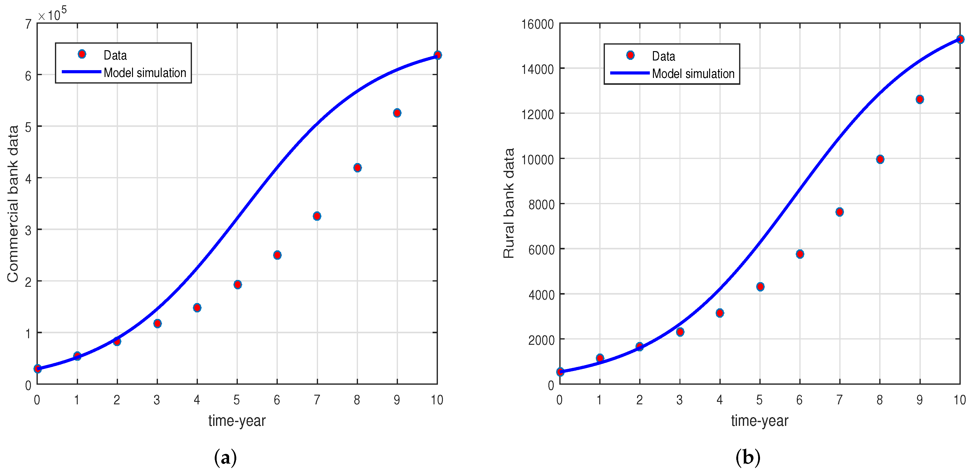
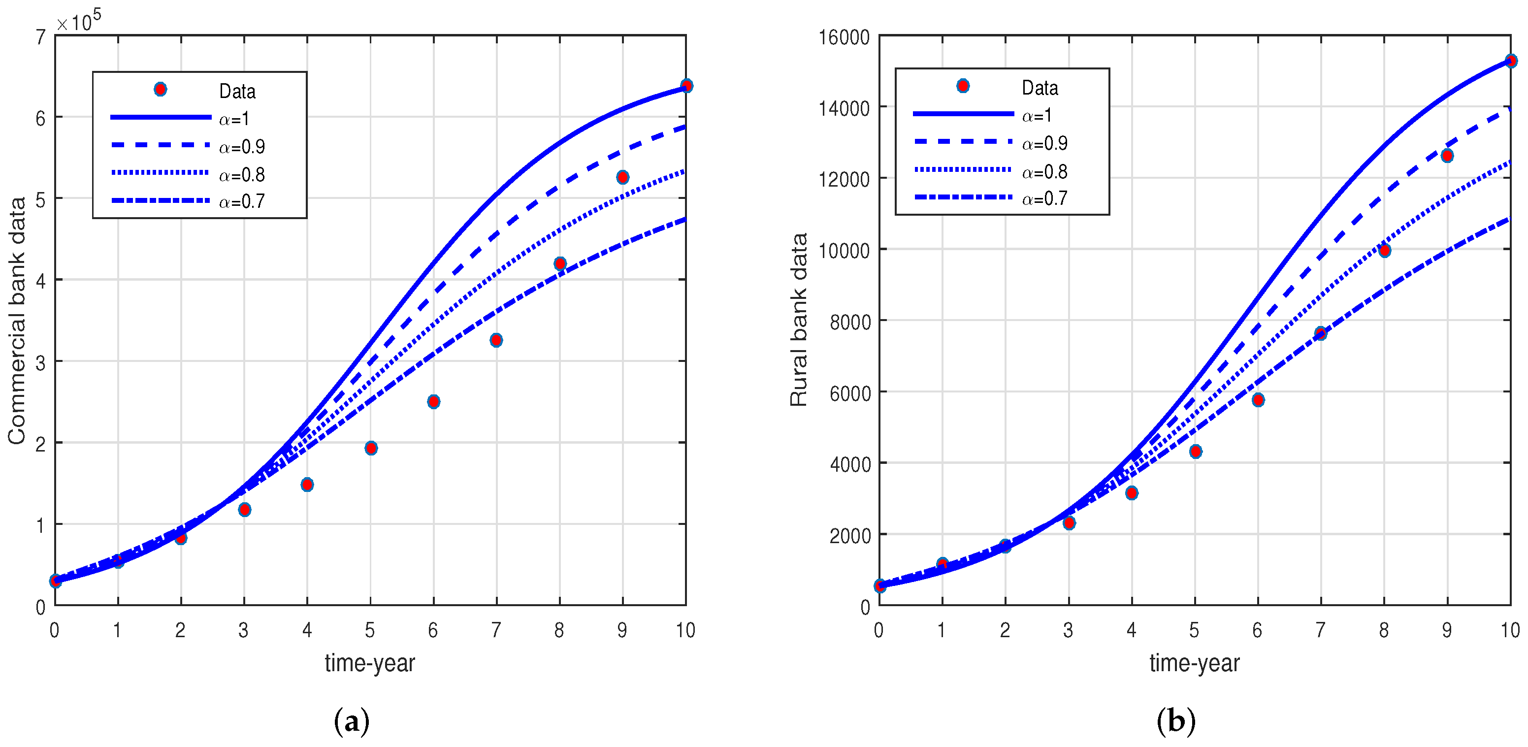
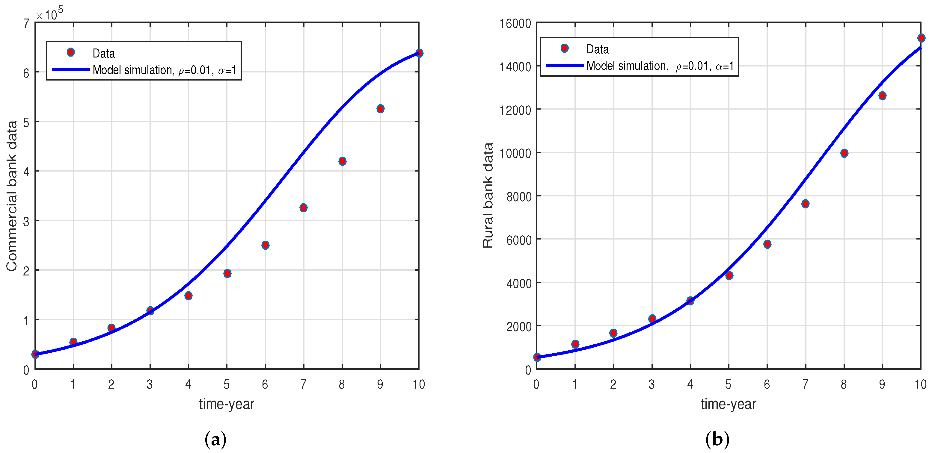
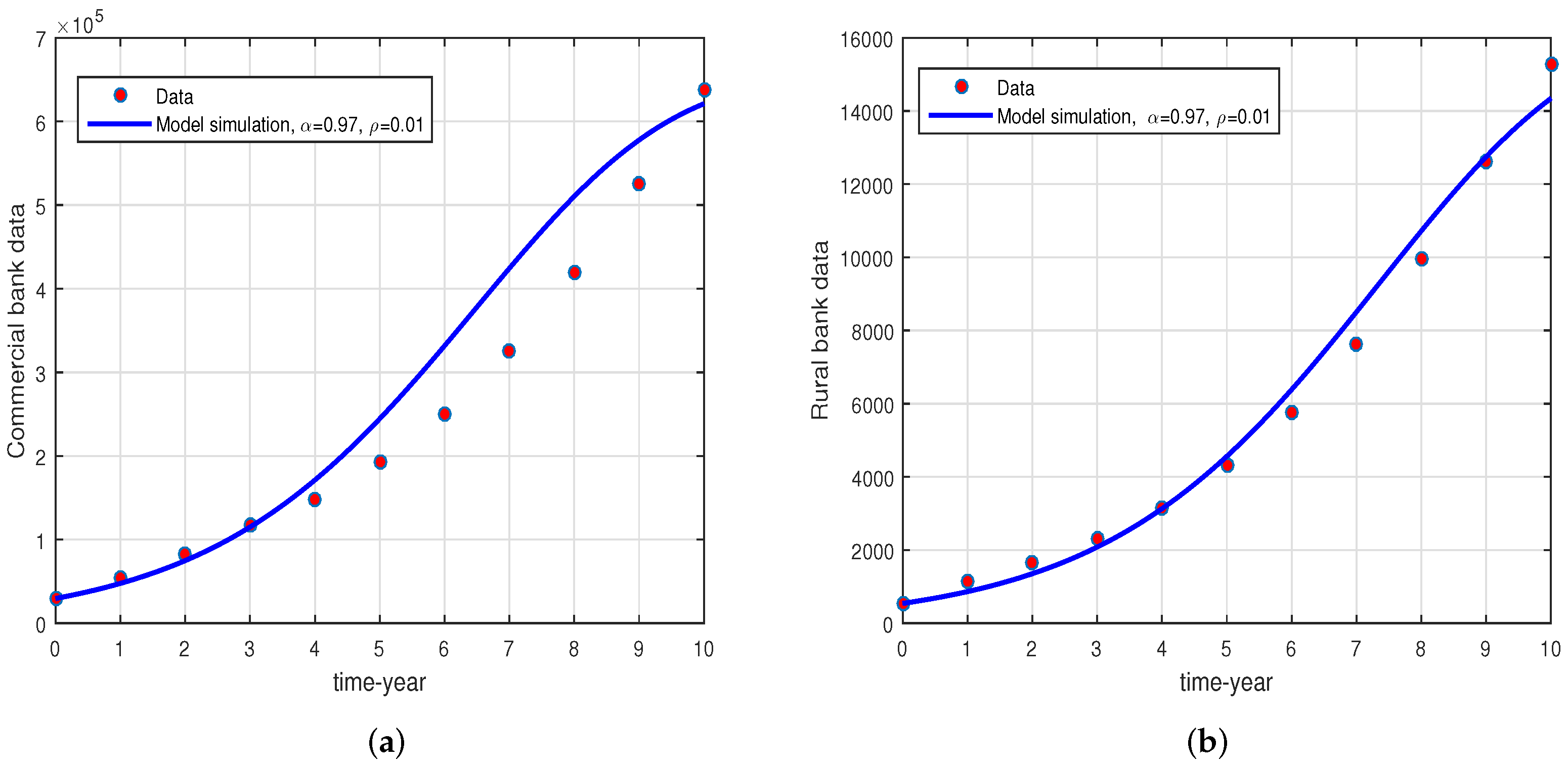
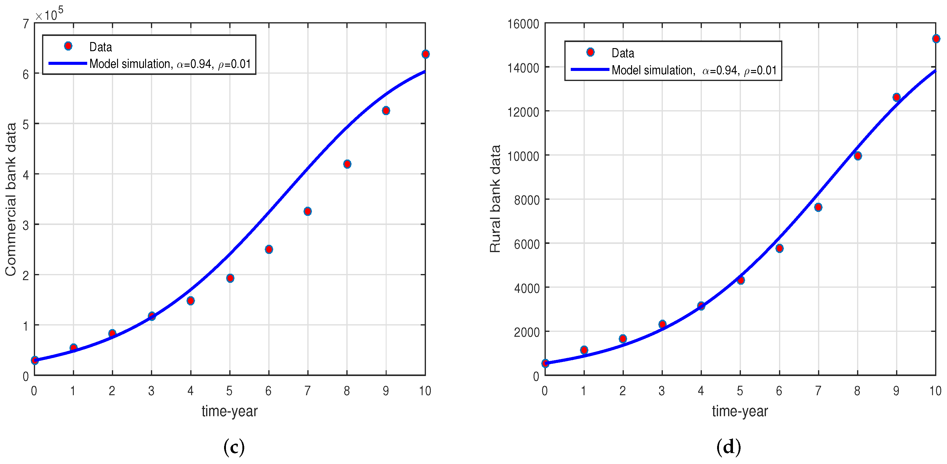
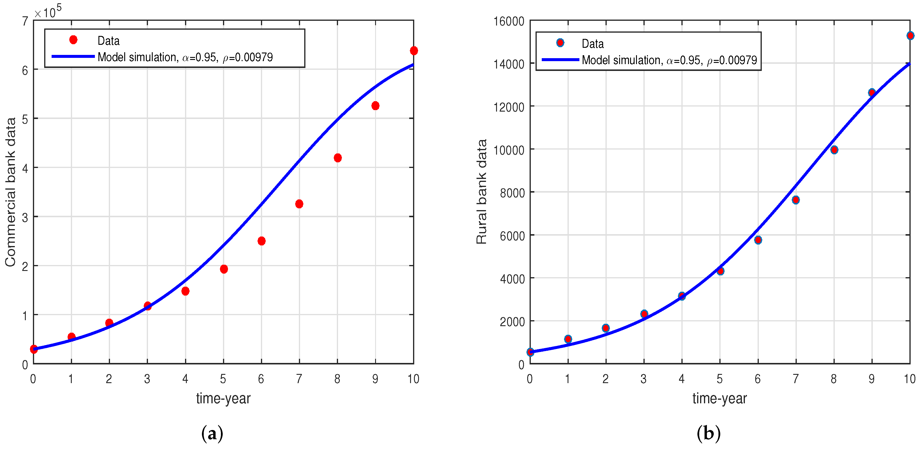
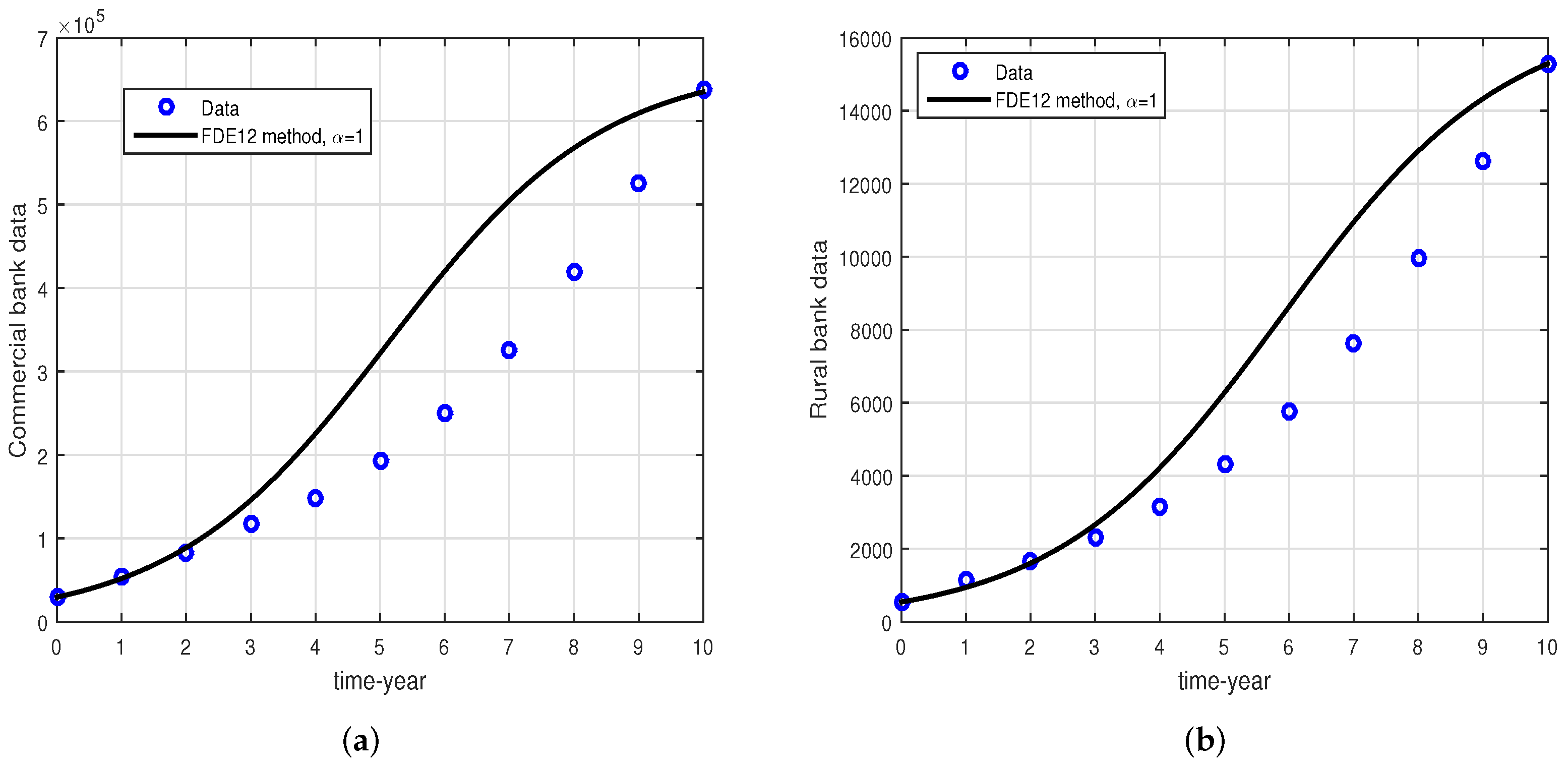
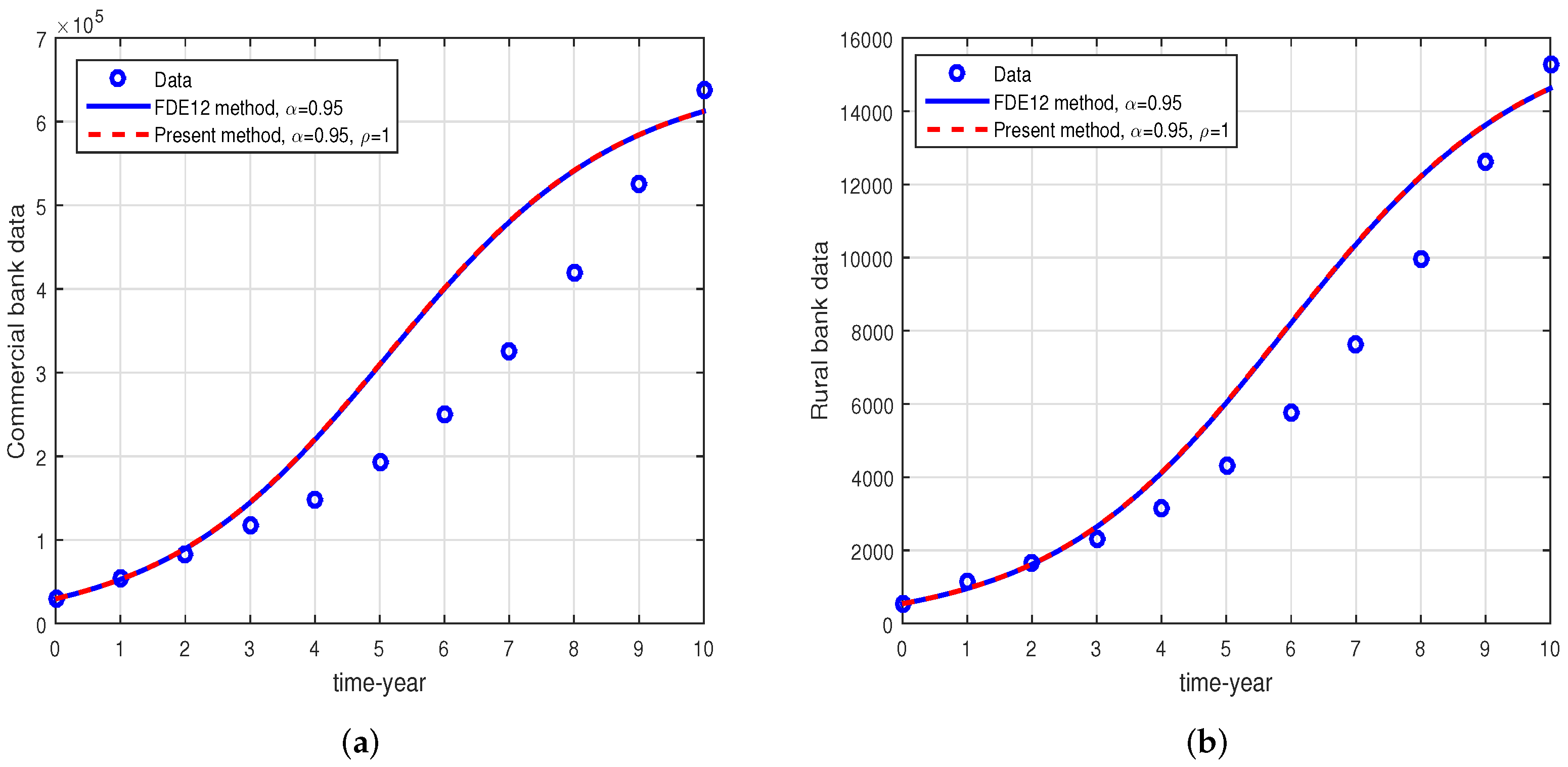
5. Numerical Results

We consider here the numerical solution of the competition model using the new and recent method introduced in the literature. One of the important advantages of this new method is the use of the ρ , which provides important results when varying its numerical values. In the present simulation, we consider the numerical values of the parameters q 1 = 2.90 × 10 10 , L 1 = 669 , 318.198 , g 1 = 0.6 , g 2 = 0.58 , q 2 = 3.9 × 10 8 and L 2 = 17 , 540.6219 , see Ref. [37], while the initial conditions of the model variables are C ( 0 ) = 29 , 463 , R ( 0 ) = 539 . The data of the two banks in Indonesia is provided by Ref. [4], and the rural and commercial data used were for the period 2004–2014. We briefly study the numerical results with the above parameters and present its comparison with various values of α and ρ and determine the best values of the fractional and parameter ρ that have a good fitting with the data.
We give Figure 1 with sub-graphs (a) and (b) that show the simulation results of commercial and rural banks when ρ = 1 and fractional order α = 1 . It can be seen that the data have a normal fitting with the model. This data fitting was considered useful when there is no fractional order model or any other useful operator.
In Figure 2, we can see that the fractional order α provides little change compared to the integer case. Regarding the variation in fractional order α and keeping ρ = 1 , the results are a little close in the case of Figure 2a, while they are a bit better for the case in Figure 2b.
In Figure 3, we consider the fractional order α = 1 and use ρ = 0.01 . We see that the results obtained in Figure 3a,b are better than the results given in Figure 1 and Figure 2. For example, we can compare the result given in Figure 1a and Figure 2a for the commercial data with the result in Figure 3a, which is obviously better from Figure 1a and Figure 2a. Similarly, the results are given in subfigures b of Figure 1 and Figure 2, and its comparison with Figure 3a, where one can see that the result given in Figure 3a is fine and better.
If we choose different values of fractional order α = 0.97 , 0.94 and keep the parameter ρ = 0.01 fixed, we get the result given in Figure 4. In subfigures a,b in Figure 4, we use the fractional order α = 0.97 and ρ = 0.01 , which indicates that the results are refining more. Similarly, for the case in subfigures c,d of Figure 4, the results of the model are much closer to the real data. It means that the variation in fractional order and the parameter ρ provides better data fitting results.
Figure 5 is given for fractional order α = 0.95 and ρ = 0.00979 . It can be observed from the graphical results that commercial and rural data have good fitting to the data and it is considered the best for this case.
We shall compare the present method with the FDE12 method used in literature for the Caputo differential equation; see Ref. [38]. We numerically solve the fractional order system (6) and show the graphical results in Figure 6, Figure 7 and Figure 8. In Figure 6, we compare the data of rural and commercial banks with the FDE12 method when α = 1 , which matched perfectly with the case in Figure 1.
The comparison of the present method with the FDE12 method for data comparison when α = 0.95 and ρ = 1 is given in Figure 7. One can see that both the methods for α = 0 , 97 provide the same results. It means that the present method is perfectly matched with the FDE-12 for α = 0.95 and for any fractional order α one can have the same result for both methods.
The comparison of the present method with FDE12 when α = 0.97 and ρ = 0.01 is given in Figure 8. Here, one can see the importance of the ρ that provides the best result compared to the FDE12 method. So, we can say that the ρ used in the present method is more powerful than FDE12.

6. Conclusions

In the present work, we considered the data of the two banks, rural and commercial, in Indonesia, and describe the profit competition among the two with the same products of the bank. We considered the previously published values of the parameters and the initial values of the variables. We considered a new method that uses an extra parameter for the factional order differential equation in Caputo case. We focused on the importance of the parameter ρ in the present work and discussed their simulation results in comparison with the real data. We presented the detailed numerical results and their discussion of the results. We utilized various aspects of the method and provided the results. We have shown that the results for ρ = 0.01 and α = 1 are more powerful than the integer order. Similarly, the results with the variations in ρ and α are better than integer orders. Here, ρ = 0.00979 and α = 0.95 are more powerful than the previous and fit the data well. This application case of banking data and its comparison using the new method of the fractional differential is reliable and useful. We compared the present method with the available method in literature, called the FDE12 method. We compared both methods for some fractional order α and found that both methods matched well. We found significantly different results for the same fractional order α and ρ = 0.01 (present method). The result of the present method was found to be better than the previous method FDE12 due to the involvement of the parameter ρ . One can utilize the method used in this work for other nonlinear problems arising in science and engineering with real data. The present method shall be considered for the case of nonlinear fractional differential equations in the case of Caputo–Fabrizio and other fractional operators for real-life problems in the future. We believe that this method is more powerful than the previous methods used in the literature. In the future, we aim to provide the result for the given model in the sense of the Atangana–Baleanu derivative and their comparison with other schemes available in the literature.

Author Contributions

Conceptualization, M.A.K.; Data curation, M.A.K. and F.; Formal analysis, M.H.D. and F.; Funding acquisition, F., M.S.A.; Investigation, M.H.D., M.A.K. and F.; Methodology, M.H.D., M.A.K., M.S.A. and F.; Resources, M.A.K.; Software, M.A.K. and F.; Validation, M.H.D., M.S.A., M.A.K. and F.; Visualization, M.S.A., M.H.D.; Writing—original draft, M.A.K. and F.; Writing—review and editing, M.S.A., M.H.D., M.A.K., and F. All authors have read and agreed to the published version of the manuscript.

Funding

The authors extend their appreciation to the Ministry of Education in KSA for funding this research work through the project number KKU-IFP2-H-8.

Data Availability Statement

Data is available from the corresponding author upon reasonable request.

Conflicts of Interest

The authors declare no conflict of interest.

References

  1. Number L of 1998 Concerning Amendment to Law Number 7 of 1992 Concerning Banking. Supplement to the State Gazette of the Republic of Indonesia. Available online: https://www.global-regulation.com/translation/indonesia/7224941/act-no.-10-of-1998.html (accessed on 10 October 2022).
  2. Arbi, S. Lembaga: Perbankan, Keuangan dan Pembiayaan. Yogyakarta: BPFE. 2013. Available online: https://opac.uinkhas.ac.id/index.php?p=show_detail&id=16217 (accessed on 10 October 2022).
  3. Iskandar, S. Bank dan Lembaga Keuangan Lainnya. 2013. Available online: https://opac.perpusnas.go.id/DetailOpac.aspx?id=992962 (accessed on 10 October 2022).
  4. Perbankan, O.J. Statistik Perbankan Indonesia 2018. 2014. Available online: https://www.ojk.go.id/id/kanal/perbankan/data-dan-statistik/statistik-perbankan-indonesia/default.aspx (accessed on 10 October 2022).
  5. Hastings, A. Population Biology: Concepts and Models; Springer: Berlin/Heidelberg, Germany, 2013. [Google Scholar]
  6. Kim, J.; Lee, D.J.; Ahn, J. A dynamic competition analysis on the Korean mobile phone market using competitive diffusion model. Comput. Ind. Eng. 2006, 51, 174–182. [Google Scholar] [CrossRef]
  7. Morris, S.A.; Pratt, D. Analysis of the Lotka–Volterra competition equations as a technological substitution model. Technol. Forecast. Soc. Chang. 2003, 70, 103–133. [Google Scholar] [CrossRef]
  8. Lee, S.J.; Lee, D.J.; Oh, H.S. Technological forecasting at the Korean stock market: A dynamic competition analysis using Lotka–Volterra model. Technol. Forecast. Soc. Chang. 2005, 72, 1044–1057. [Google Scholar] [CrossRef]
  9. Michalakelis, C.; Christodoulos, C.; Varoutas, D.; Sphicopoulos, T. Dynamic estimation of markets exhibiting a prey–predator behavior. Expert Syst. Appl. 2012, 39, 7690–7700. [Google Scholar] [CrossRef]
  10. Lakka, S.; Michalakelis, C.; Varoutas, D.; Martakos, D. Competitive dynamics in the operating systems market: Modeling and policy implications. Technol. Forecast. Soc. Chang. 2013, 80, 88–105. [Google Scholar] [CrossRef]
  11. Comes, C.A. Banking system: Three level Lotka-Volterra model. Procedia Econ. Financ. 2012, 3, 251–255. [Google Scholar] [CrossRef] [Green Version]
  12. Fatmawati, M.A.; Azizah, M.; Ullah, S. A fractional model for the dynamics of competition between commercial and rural banks in Indonesia. Chaos Solitons Fractals 2019, 122, 32–46. [Google Scholar] [CrossRef]
  13. Wang, W.; Khan, M.A.; Kumam, P.; Thounthong, P. A comparison study of bank data in fractional calculus. Chaos Solitons Fractals 2019, 126, 369–384. [Google Scholar] [CrossRef]
  14. Li, Z.; Liu, Z.; Khan, M.A. Fractional investigation of bank data with fractal-fractional Caputo derivative. Chaos Solitons Fractals 2020, 131, 109528. [Google Scholar] [CrossRef]
  15. Wang, W.; Khan, M.A. Analysis and numerical simulation of fractional model of bank data with fractal–fractional Atangana–Baleanu derivative. J. Comput. Appl. Math. 2020, 369, 112646. [Google Scholar] [CrossRef]
  16. Gavin, C.; Pokrovskii, A.; Prentice, M.; Sobolev, V. Dynamics of a Lotka-Volterra type model with applications to marine phage population dynamics. J. Phys. Conf. Ser. 2006, 55, 8. [Google Scholar] [CrossRef]
  17. Aboites, V.; Bravo-Avilés, J.F.; García-López, J.H.; Jaimes-Reategui, R.; Huerta-Cuellar, G. Interpretation and Dynamics of the Lotka–Volterra Model in the Description of a Three-Level Laser. Photonics 2021, 9, 16. [Google Scholar] [CrossRef]
  18. Hung, H.C.; Chiu, Y.C.; Huang, H.C.; Wu, M.C. An enhanced application of Lotka–Volterra model to forecast the sales of two competing retail formats. Comput. Ind. Eng. 2017, 109, 325–334. [Google Scholar] [CrossRef]
  19. Hsu, S.B.; Zhao, X.Q. A Lotka–Volterra competition model with seasonal succession. J. Math. Biol. 2012, 64, 109–130. [Google Scholar] [CrossRef]
  20. Dimas Martins, A.; Gjini, E. Modeling competitive mixtures with the Lotka-Volterra framework for more complex fitness assessment between strains. Front. Microbiol. 2020, 11, 572487. [Google Scholar] [CrossRef]
  21. Ullah, S.; Khan, M.A.; Farooq, M. A fractional model for the dynamics of TB virus. Chaos Solitons Fractals 2018, 116, 63–71. [Google Scholar] [CrossRef]
  22. Podlubny, I. An introduction to fractional derivatives, fractional differential equations, to methods of their solution and some of their applications. Math. Sci. Eng 1999, 198, 340. [Google Scholar]
  23. Das, S.; Gupta, P. A mathematical model on fractional Lotka–Volterra equations. J. Theor. Biol. 2011, 277, 1–6. [Google Scholar] [CrossRef]
  24. Khan, M.A.; Hammouch, Z.; Baleanu, D. Modeling the dynamics of hepatitis E via the Caputo–Fabrizio derivative. Math. Model. Nat. Phenom. 2019, 14, 311. [Google Scholar] [CrossRef]
  25. Khan, M.A.; Ullah, S.; Farooq, M. A new fractional model for tuberculosis with relapse via Atangana–Baleanu derivative. Chaos Solitons Fractals 2018, 116, 227–238. [Google Scholar] [CrossRef]
  26. Shaiful, E.M.; Utoyo, M.I. A fractional-order model for HIV dynamics in a two-sex population. Int. J. Math. Math. Sci. 2018, 2018, 6801475. [Google Scholar]
  27. Atangana, A.; Nieto, J.J. Numerical solution for the model of RLC circuit via the fractional derivative without singular kernel. Adv. Mech. Eng. 2015, 7, 1687814015613758. [Google Scholar] [CrossRef]
  28. Abaid Ur Rehman, M.; Ahmad, J.; Hassan, A.; Awrejcewicz, J.; Pawlowski, W.; Karamti, H.; Alharbi, F.M. The Dynamics of a Fractional-Order Mathematical Model of Cancer Tumor Disease. Symmetry 2022, 14, 1694. [Google Scholar] [CrossRef]
  29. Lan, Y.; Shi, J.; Fang, H. Hopf Bifurcation and Control of a Fractional-Order Delay Stage Structure Prey-Predator Model with Two Fear Effects and Prey Refuge. Symmetry 2022, 14, 1408. [Google Scholar] [CrossRef]
  30. Yang, X.; Su, Y.; Li, H.; Zhuo, X. Optimal Control of a Cell-to-Cell Fractional-Order Model with Periodic Immune Response for HCV. Symmetry 2021, 13, 2121. [Google Scholar] [CrossRef]
  31. Askar, S.; Al-Khedhairi, A.; Elsonbaty, A.; Elsadany, A. Chaotic discrete fractional-order food chain model and hybrid image encryption scheme Application. Symmetry 2021, 13, 161. [Google Scholar] [CrossRef]
  32. Diouf, M.; Sene, N. Analysis of the financial chaotic model with the fractional derivative operator. Complexity 2020, 2020, 9845031. [Google Scholar] [CrossRef]
  33. Mahdy, A.M.; Amer, Y.A.E.; Mohamed, M.S.; Sobhy, E. General fractional financial models of awareness with Caputo–Fabrizio derivative. Adv. Mech. Eng. 2020, 12, 1687814020975525. [Google Scholar] [CrossRef]
  34. Xu, C.; Aouiti, C.; Liao, M.; Li, P.; Liu, Z. Chaos control strategy for a fractional-order financial model. Adv. Differ. Eq. 2020, 2020, 1–17. [Google Scholar] [CrossRef]
  35. Atangana, A.; Araz, S.I. A modified parametrized method for ordinary differential equations with nonlocal operators, hal-03840759, Hal Open science. 2022.
  36. Caputo, M. Linear models of dissipation whose Q is almost frequency independent II. Geophys. J. Int. 1967, 13, 529–539. [Google Scholar] [CrossRef]
  37. Atangana, A.; Khan, M.A.; Fatmawati. Modeling and analysis of competition model of bank data with fractal-fractional Caputo-Fabrizio operator. Alex. Eng. J. 2020, 59, 1985–1998. [Google Scholar] [CrossRef]
  38. Diethelm, K.; Freed, A.D. The FracPECE subroutine for the numerical solution of differential equations of fractional order. Forsch. Wiss. Rechn. 1998, 1999, 57–71. [Google Scholar]
Figure 1. Real data of commercial and rural banks versus model for ρ = 1 (a) commercial, (b) rural.
Symmetry 15 00542 g001
Figure 2. Fitting of data versus the model for various values α and ρ = 1 , (a) commercial, (b) rural.
Symmetry 15 00542 g002
Figure 3. Data versus model comparison when α = 1 , and ρ = 0.01 (a) commercial banks, (b) rural banks.
Symmetry 15 00542 g003
Figure 4. Comparison results of data versus model comparison when α = 0.97 , 0.94 , and ρ = 0.01 sub-graph (a,c) describes the commercial banks, while (b,d) is for rural banks.
Symmetry 15 00542 g004aSymmetry 15 00542 g004b
Figure 5. Comparison results of data versus model when α = 0.95 and ρ = 0.00979 . (a) gives the comparison of model versus commercial bank data when α = 0.95 and ρ = 0.00979 while (b) gives the comparison of model versus rural bank data when α = 0.95 and ρ = 0.00979 .
Symmetry 15 00542 g005
Figure 6. FDE12 method comparison with real data of commercial and rural. Figures (a,b) respectively give the comparison of the FDE12 method with data when α = 1 .
Symmetry 15 00542 g006
Figure 7. Comparison of FDE12 and the present method for data comparison when α = 0.95 and ρ = 1 , where (a) denotes commercial data while (b) rural data.
Symmetry 15 00542 g007
Figure 8. Comparison of FDE12 and present method for data comparison when α = 0.97 and ρ = 0.01 , where (a) defines commercial banks while (b) defines rural banks.
Symmetry 15 00542 g008
Disclaimer/Publisher’s Note: The statements, opinions and data contained in all publications are solely those of the individual author(s) and contributor(s) and not of MDPI and/or the editor(s). MDPI and/or the editor(s) disclaim responsibility for any injury to people or property resulting from any ideas, methods, instructions or products referred to in the content.

