
Modified Exp-Function Method to Find Exact Solutions of Microtubules Nonlinear Dynamics Models

Abstract
:1. Introduction
- (i)
- The nonlinear PDE describes the model of microtubule nonlinear dynamics assum-ing a single longitudinal degree of freedom per tubulin dimer (see [38]),
- (ii)
- The nonlinear PDE explaining the radially displaced MTs’ nonlinear dynamics:
2. The Portrayal of the Method
- a.
- When
- b.
- When
- c.
- When
- d.
- When
- e.
- When
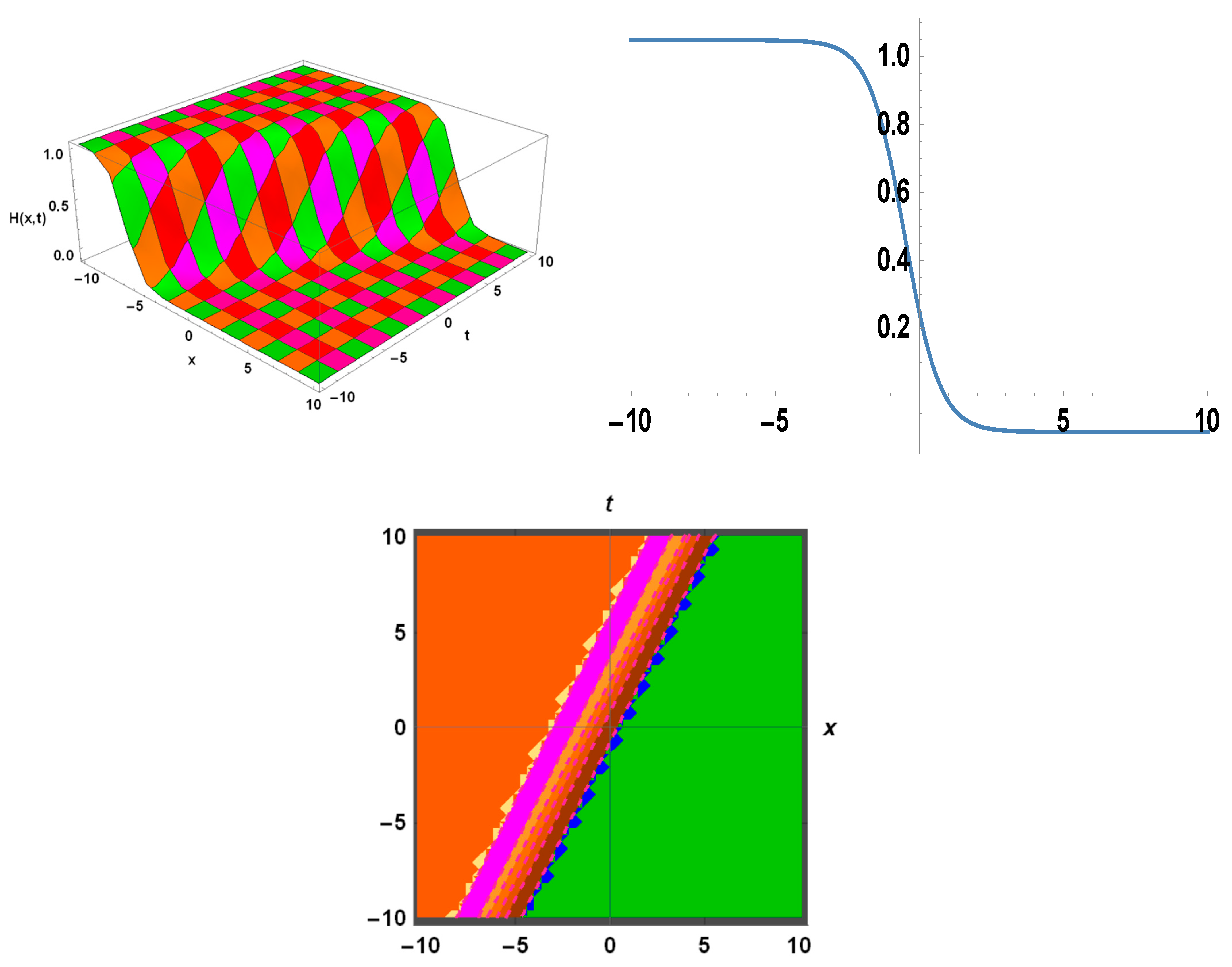
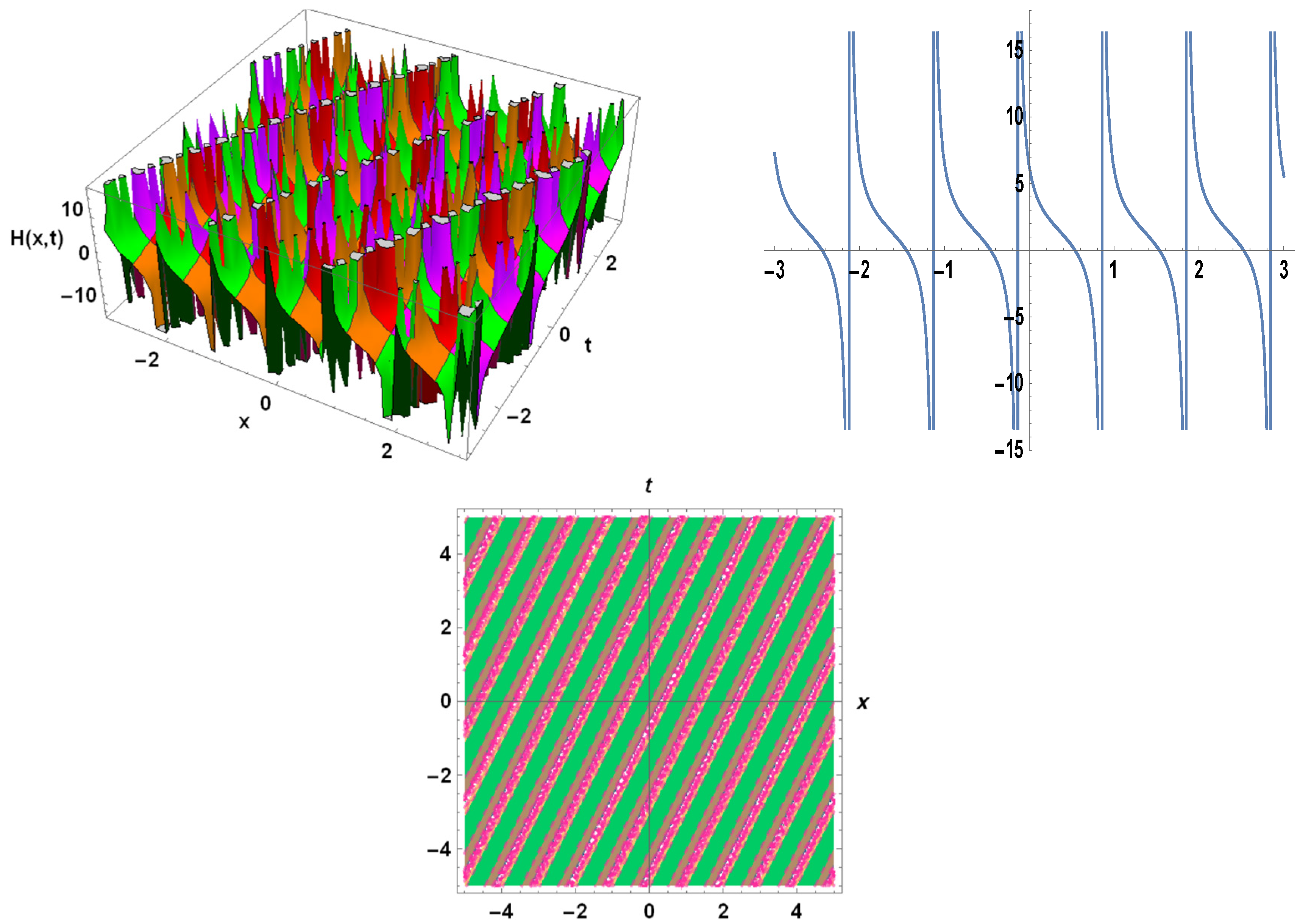
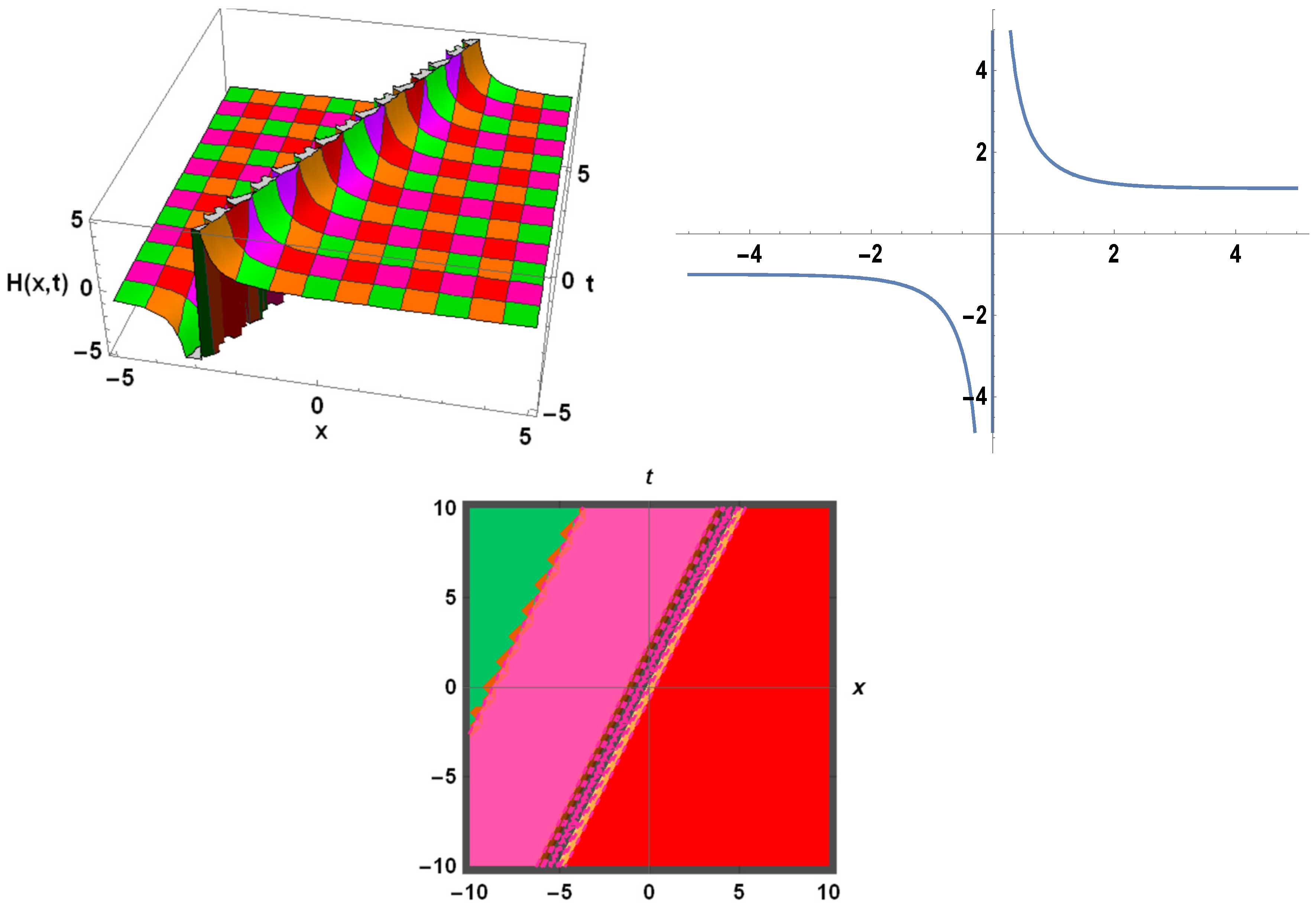
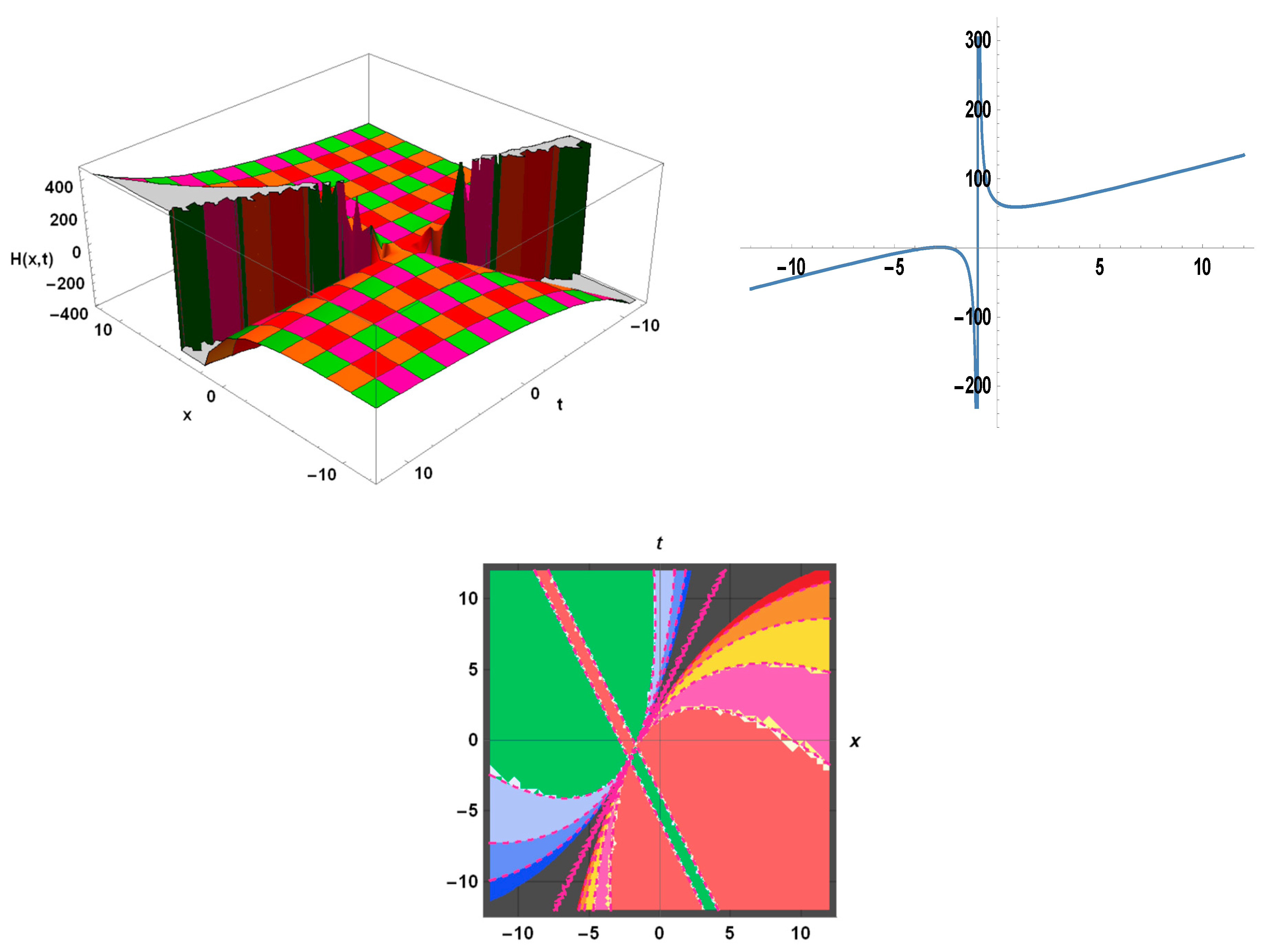
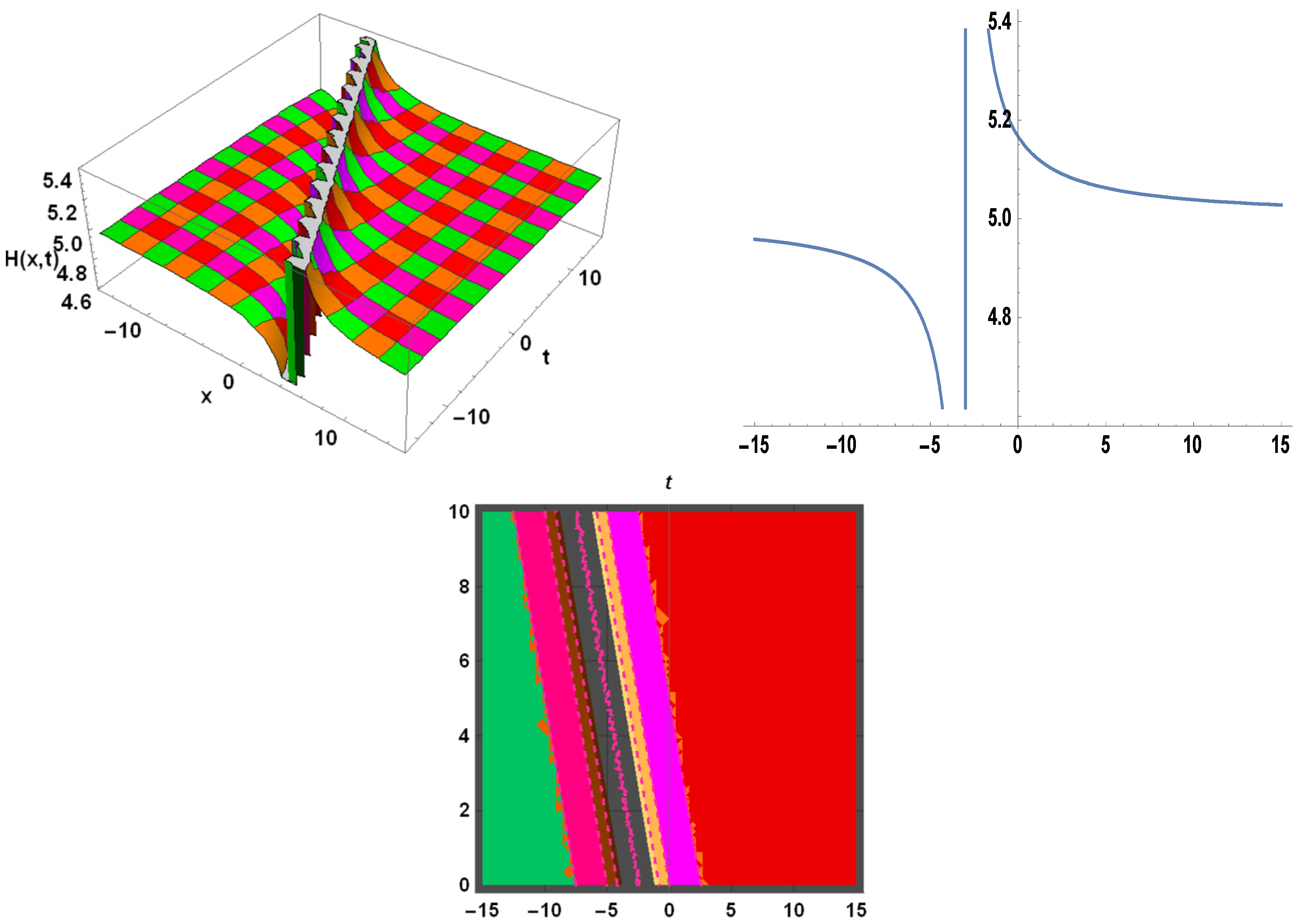
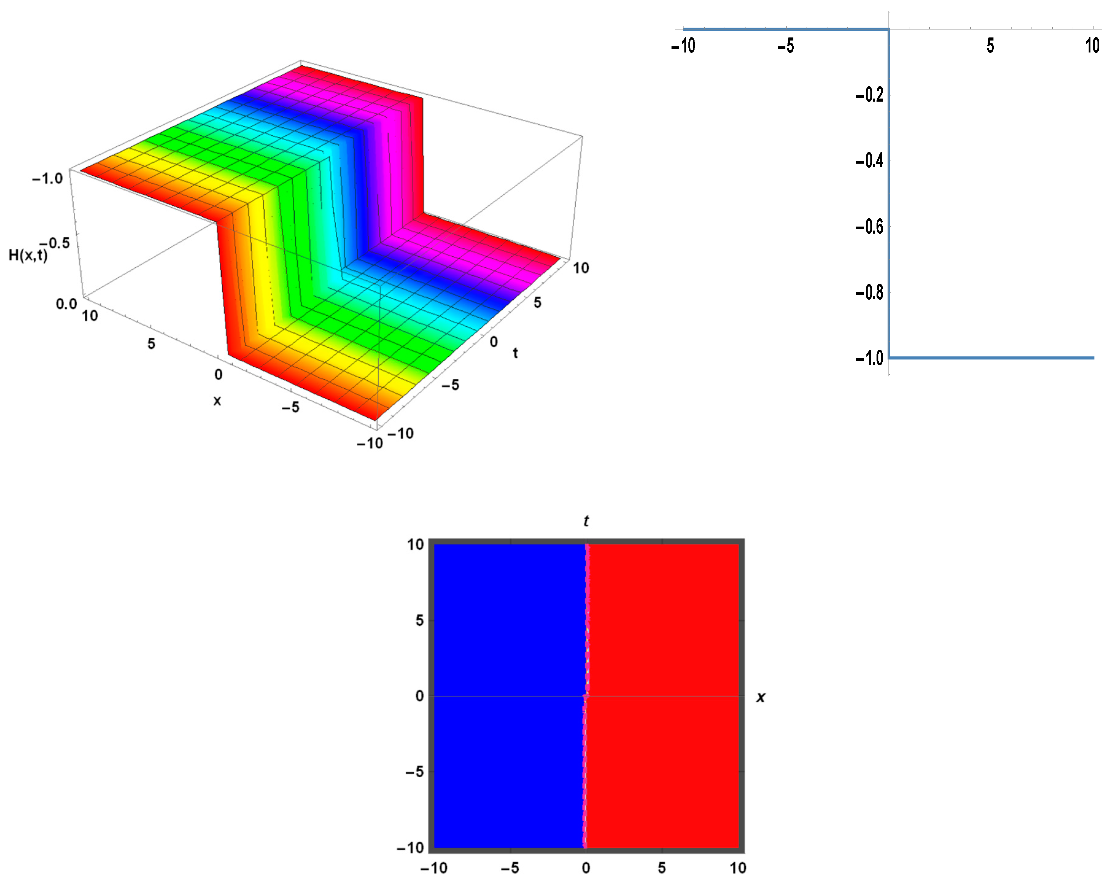
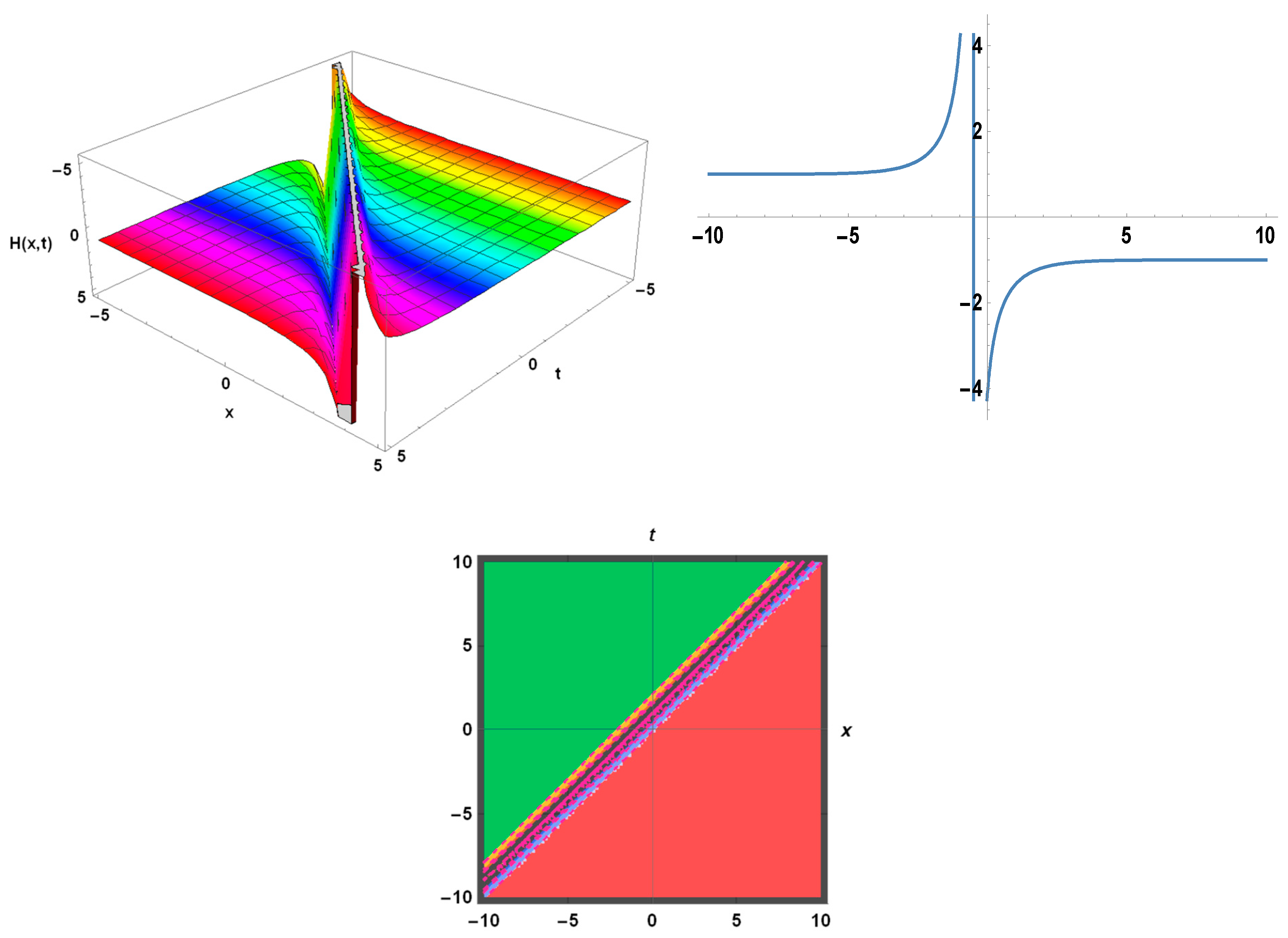
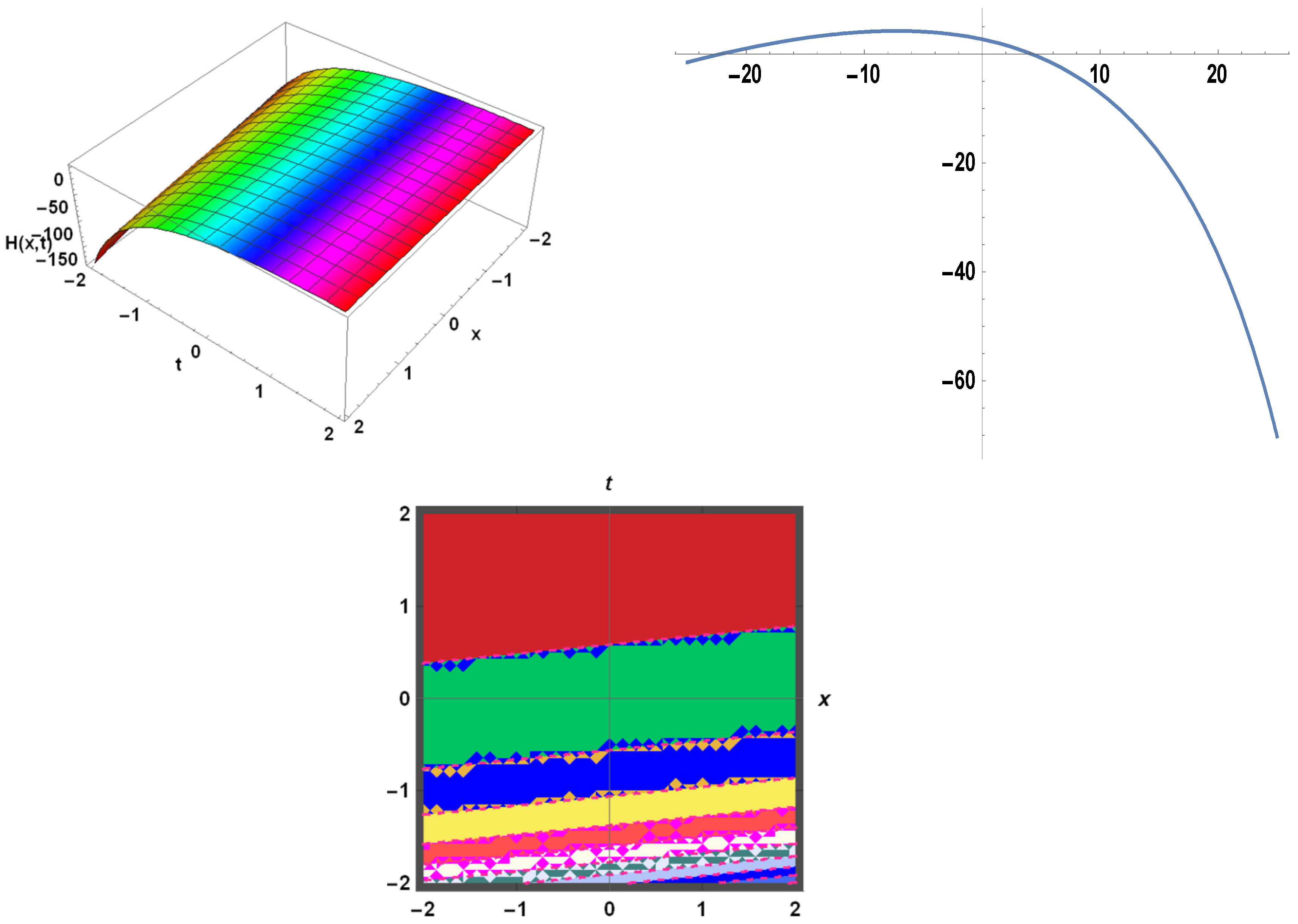
3. Applications
4. Physical Expression of the Problem
5. Conclusions
Author Contributions
Funding
Data Availability Statement
Acknowledgments
Conflicts of Interest
References
- Jafar, B.; Asadi, M.A.; Salehi, F. Rational Homotopy Perturbation Method for solving stiff systems of ordinary differential equations. Appl. Math. Model. 2015, 39, 1291–1299. [Google Scholar]
- Cariello, F.; Tabor, M. Painlevé expansions for nonintegrable evolution equations. Phys. D Nonlinear Phenom. 1989, 39, 77–94. [Google Scholar] [CrossRef]
- Philip, D.G.; Drazin, P.G.; Johnson, R.S. Solitons: An Introduction; No. 2; Cambridge University Press: Cambridge, UK, 1989. [Google Scholar]
- Aslam, M.N.; Akbar, M.A.; Mohyud-Din, S.T. General traveling wave solutions of the strain wave equation in microstructured solids via the new approach of generalized (G′/G)-expansion method. Alex. Eng. J. 2014, 53, 233–241. [Google Scholar] [CrossRef] [Green Version]
- Shakeel, M.; Ul-Hassan, Q.M.; Ahmad, J.; Naqvi, T. Exact solutions of the time fractional BBM-Burger equation by novel (𝐺′/𝐺)-expansion method. Adv. Math. Phys. 2014, 2014, 181594. [Google Scholar] [CrossRef] [Green Version]
- Zhou, Y.; Wang, M.; Wang, Y. Periodic wave solutions to a coupled KdV equations with variable coefficients. Phys. Lett. A 2003, 308, 31–36. [Google Scholar] [CrossRef]
- Ali, A.T. New generalized Jacobi elliptic function rational expansion method. J. Comput. Appl. Math. 2011, 235, 4117–4127. [Google Scholar] [CrossRef] [Green Version]
- Lü, D. Jacobi elliptic function solutions for two variant Boussinesq equations. Chaos Solitons Fractals 2005, 24, 1373–1385. [Google Scholar] [CrossRef]
- Liu, S.; Fu, Z.; Liu, S.; Zhao, Q. Jacobi elliptic function expansion method and periodic wave solutions of nonlinear wave equations. Phys. Lett. A 2001, 289, 69–74. [Google Scholar] [CrossRef]
- Fan, E. Two new applications of the homogeneous balance method. Phys. Lett. A 2000, 265, 353–357. [Google Scholar] [CrossRef]
- Fan, E. Extended tanh-function method and its applications to nonlinear equations. Phys. Lett. A 2000, 277, 212–218. [Google Scholar] [CrossRef]
- Soliman, A.A. The modified extended tanh-function method for solving Burgers-type equations. Phys. A Stat. Mech. Its Appl. 2006, 361, 394–404. [Google Scholar] [CrossRef]
- Li, Z.; Liu, Y. RATH: A Maple package for finding travelling solitary wave solutions to nonlinear evolution equations. Comput. Phys. Commun. 2002, 148, 256–266. [Google Scholar] [CrossRef]
- Peng, Y.Z. A mapping method for obtaining exact travelling wave solutions to nonlinear evolution equations. Chin. J. Phys. 2003, 41, 103–110. [Google Scholar]
- Yomba, E. Construction of new soliton-like solutions of the (2+ 1) dimensional dispersive long wave equation. Chaos Solitons Fractals 2004, 20, 1135–1139. [Google Scholar] [CrossRef]
- Alam, N.; Alam, M.M. An analytical method for solving exact solutions of a nonlinear evolution equation describing the dynamics of ionic currents along microtubules. J. Taibah Univ. Sci. 2017, 11, 939–948. [Google Scholar] [CrossRef]
- MAlam, N.; Hafez, M.G.; Akbar, M.A.; Roshid, H.O. Exact traveling wave solutions to the (3+1)-dimensional mKdV-ZK and the (2+1)-dimensional Burgers equations via exp (-Eta)-expansion method. Alex. Eng. J. 2015, 54, 635–644. [Google Scholar]
- Roshid, H.O.; Alam, M.N.; Akbar, M.A. Traveling wave solutions for fifth order (1+1)-dimensional Kaup-Keperschmidt equation with the help of exp(−Φ(ξ))-expansion method. Walailak J. Sci. Technol. 2015, 12, 1063–1073. [Google Scholar]
- Alam, M.N.; Hafez, M.G.; Akbar, M.A.; Roshid, H.O. Exact solutions to the (2+1)-dimensional Boussinesq equation via exp(−Φ(ξ))-expansion method. J. Sci. Res. 2015, 7, 1–10. [Google Scholar] [CrossRef] [Green Version]
- Alam, M.N.; Belgacem, F.B.M. Microtubules nonlinear models dynamics investigations through the exp(−Φ(ξ))-expansion method implementation. Mathematics 2016, 4, 6. [Google Scholar] [CrossRef]
- Shakeel, M.; Mohyud-Din, S.T.; Iqbal, M.A. Closed form solutions for coupled nonlinear Maccari system. Comput. Math. Appl. 2018, 76, 799–809. [Google Scholar] [CrossRef]
- Liu, H.-Z. An equivalent form for the exp(−Φ(ξ))-expansion method. Jpn. J. Ind. Appl. Math. 2018, 35, 1153–1161. [Google Scholar] [CrossRef]
- Jeffrey, A.; Mohamad, M.N.B. Exact solutions to the KdV-Burgers’ equation. Wave Motion 1991, 14, 369–375. [Google Scholar] [CrossRef]
- Jin, T.; Yang, X. Monotonicity theorem for the uncertain fractional differential equation and application to uncertain financial market. Math. Comput. Simul. 2021, 190, 203–221. [Google Scholar] [CrossRef]
- Jin, T.; Yang, X.; Xia, H.; Ding, H. Reliability index and option pricing formulas of the first hitting time model based on the uncertain fractional-order differential equation with Caputo type. Fractals 2021, 29, 2150001. [Google Scholar] [CrossRef]
- Tian, C.; Jina, T.; Yang, X.; Liu, Q. Reliability analysis of the uncertain heat conduction model. Comput. Math. Appl. 2022, 119, 131–140. [Google Scholar] [CrossRef]
- Bai, X.; Shi, H.; Zhang, K.; Zhang, X.; Wu, Y. Effect of the fit clearance between ceramic outer ring and steel pedestal on the sound radiation of full ceramic ball bearing system. J. Sound Vib. 2022, 529, 116967. [Google Scholar] [CrossRef]
- Li, S.; Liu, Z. Scheduling uniform machines with restricted assignment. Math. Biosci. Eng. 2022, 19, 9697–9708. [Google Scholar] [CrossRef]
- Shao, Z.; Zhai, Q.; Han, Z.; Guan, X. A linear AC unit commitment formulation: An application of data-driven linear power flow model. Int. J. Electr. Power Energy Syst. 2023, 145, 108673. [Google Scholar] [CrossRef]
- Sataric, M.V.; Sekulic, D.L.; Sataric, B.M.; Zdravkovic, S. Role of nonlinear localized Ca2+ pulses along microtubules in tuning the mechano-Sensitivity of hair cells. Prog. Biophys. Mol. Biol. 2015, 119, 162–174. [Google Scholar] [CrossRef]
- Sekulic, D.; Sataric, M.V. An improved nanoscale transmission line model of microtubules: The effect of nonlinearity on the propagation of electrical signals. Facta Univ. Ser. Electron. Energ. 2015, 28, 133–142. [Google Scholar] [CrossRef] [Green Version]
- Sekulic, D.L.; Sataric, B.M.; Tuszynski, J.A.; Sataric, M.V. Nonlinear ionic pulses along microtubules. Eur. Phys. J. E Soft Matter 2011, 34, 49. [Google Scholar] [CrossRef] [PubMed]
- Sekulic, D.; Sataric, M.V.; Zivanov, M.B. Symbolic computation of some new nonlinear partial differential equations of nanobiosciences using modified extended tanh-function method. Appl. Math. Comput. 2011, 218, 3499–3506. [Google Scholar] [CrossRef]
- Sataric, M.V.; Sekulic, D.; Zivanov, M.B. Solitonic ionic currents along microtubules. J. Comput. Theor. Nanosci. 2010, 7, 2281–2290. [Google Scholar] [CrossRef]
- Zayed, E.M.E.; Alurrfi, K.A.E. The generalized projective Riccati equations method and its applications for solving two nonlinear PDEs describing microtubules. Int. J. Phys. Sci. 2015, 10, 391–402. [Google Scholar]
- Sekulic, D.L.; Sataric, M.V. Microtubule as Nanobioelectronic nonlinear circuit. Serb. J. Electr. Eng. 2012, 9, 107–119. [Google Scholar] [CrossRef]
- Zdravkovic, S.; Sataric, M.V.; Maluckov, A.; Balaz, A. A nonlinear model of the dynamics of radial dislocations in microtubules. Appl. Math. Comput. 2014, 237, 227–237. [Google Scholar] [CrossRef]
- Zdravkovic, S.; Sataric, M.V.; Zekovic, S. Nonlinear dynamics of microtibules-A longitudinal model. Europhys. Lett. 2013, 102, 38002. [Google Scholar] [CrossRef] [Green Version]
- Zekovic, S.; Muniyappan, A.; Zdravkovic, S.; Kavitha, L. Employment of Jacobian elliptic functions for solving problems in nonlinear dynamics of microtubules. Chin. Phys. B 2015, 23, 020504. [Google Scholar] [CrossRef] [Green Version]
- Shakeel, M.; Iqbal, M.A.; Din, Q.; Hassan, Q.M.; Ayub, K. New exact solutions for coupled nonlinear system of ion sound and Langmuir waves. Indian J. Phys. 2020, 94, 885–894. [Google Scholar] [CrossRef]
- Weisstein, E.W. Concise Encyclopedia of Mathematics, 2nd ed.; CRC: New York, NY, USA, 2002. [Google Scholar]


| Our Solutions | Solutions by Alam and Belgacem [20] |
|---|---|
| If we put and in our solution (18), then | If we put in solution (24), then |
| If we put and in our solution (19), then | If we put in solution (25), then |
| If we put and in our solution (20), then | If we put in solution (26), then |
| If we put and in our solution (21), then | If we put in solution (27), then |
| If we put and in our solution (22), then | If we put in solution (28), then |
| If we put and in our solution (28), then | If we put in solution (41), then |
| If we put and in our solution (29), then | If we put in solution (41), then |
| If we put and in our solution (30), then | If we put in solution (43), then |
| If we put and in our solution (31), then | If we put in solution (44), then |
| If we put and in our solution (32), then | If we put in solution (45), then |
Disclaimer/Publisher’s Note: The statements, opinions and data contained in all publications are solely those of the individual author(s) and contributor(s) and not of MDPI and/or the editor(s). MDPI and/or the editor(s) disclaim responsibility for any injury to people or property resulting from any ideas, methods, instructions or products referred to in the content. |
© 2023 by the authors. Licensee MDPI, Basel, Switzerland. This article is an open access article distributed under the terms and conditions of the Creative Commons Attribution (CC BY) license (https://creativecommons.org/licenses/by/4.0/).
Share and Cite
Shakeel, M.; Attaullah; Shah, N.A.; Chung, J.D. Modified Exp-Function Method to Find Exact Solutions of Microtubules Nonlinear Dynamics Models. Symmetry 2023, 15, 360. https://doi.org/10.3390/sym15020360
Shakeel M, Attaullah, Shah NA, Chung JD. Modified Exp-Function Method to Find Exact Solutions of Microtubules Nonlinear Dynamics Models. Symmetry. 2023; 15(2):360. https://doi.org/10.3390/sym15020360
Chicago/Turabian StyleShakeel, Muhammad, Attaullah, Nehad Ali Shah, and Jae Dong Chung. 2023. "Modified Exp-Function Method to Find Exact Solutions of Microtubules Nonlinear Dynamics Models" Symmetry 15, no. 2: 360. https://doi.org/10.3390/sym15020360