Jacobi and Lyapunov Stability Analysis of Circular Geodesics around a Spherically Symmetric Dilaton Black Hole

Abstract

We analyze the stability of the geodesic curves in the geometry of the Gibbons–Maeda–Garfinkle–Horowitz–Strominger black hole, describing the space time of a charged black hole in the low energy limit of the string theory. The stability analysis is performed by using both the linear (Lyapunov) stability method, as well as the notion of Jacobi stability, based on the Kosambi–Cartan–Chern theory. Brief reviews of the two stability methods are also presented. After obtaining the geodesic equations in spherical symmetry, we reformulate them as a two-dimensional dynamic system. The Jacobi stability analysis of the geodesic equations is performed by considering the important geometric invariants that can be used for the description of this system (the nonlinear and the Berwald connections), as well as the deviation curvature tensor, respectively. The characteristic values of the deviation curvature tensor are specifically calculated, as given by the second derivative of effective potential of the geodesic motion. The Lyapunov stability analysis leads to the same results. Hence, we can conclude that, in the particular case of the geodesic motion on circular orbits in the Gibbons–Maeda–Garfinkle–Horowitz–Strominger, the Lyapunov and the Jacobi stability analysis gives equivalent results.

1. Introduction

The analysis of the global stability of the solutions of the systems of strongly nonlinear, first or second order differential equations, describing the temporal evolution of complicated dynamical systems, is usually performed in the framework of a rigorous mathematical approach, with the help of the well known, and mathematically extensively investigated Lyapunov stability theory. In this commonly accepted approach to the problem of the stability of the solutions of differential equations, the basic mathematical quantities to be studied are the Lyapunov exponents. The Lyapunov exponents determine the exponential departures of the trajectories, obtained as solutions of the differential equations describing a given dynamical system, as compared to a standard trajectory, taken as reference [1,2]. However, when one attempts to obtain the Lyapunov exponents, one must understand that generally it is a very complicated task to find them in an exact analytical form. For that reason, in order to evaluate the basic Lyapunov exponents, and their properties, one should apply mostly complicated numerical methods. Currently, a large number of powerful numerical methods have been established for their calculation. Such numerical methods are extensively used for the mathematical, as well as physical description of the temporal evolution near the critical points of the differential equations describing dynamical systems [3,4].

The mathematical approach based on the Lyapunov linear stability analysis is well developed from a mathematical point of view. Moreover, it provides an intuitive and clear comprehension of some of the stability properties of the systems of differential equations. Nevertheless, to obtain a more profound understanding of the time evolution and general properties of the natural and mathematical structures, alternative approaches for the investigation of the stability problems must also be proposed, examined, and fully investigated. Hence, after a new method for the study of the stability is developed, one could contrast exhaustively the results, predictions, and the possible shortcomings of the newly introduced method with the consequences and conclusions gained by adopting the linear Lyapunov stability analysis of the considered system of differential equations.

One of the alternative approaches to the problem of stability that could provide valuable information for the investigation of the stability of the systems of ordinary second order differential equations is given by what one could designate as the geometro-dynamical approach. Historically, one of the first illustrations of such a different mathematical investigation of the stability problem of the systems of differential equations is the Kosambi–Cartan–Chern (KCC) theory. In its early formulation, the KCC theory was developed in the major investigations of Kosambi [5], Cartan [6] and Chern [7], respectively, which led to a first rigorous mathematical investigation of the geometric properties of dynamical systems. From a strictly mathematical perspective, the KCC theory is strongly influenced by the geometry of the Finsler spaces, which largely represents, and significantly contributed, to its theoretical justification. The KCC theory is built up by using the basic conjecture according to which there is a mathematical analogy between autonomous or non-autonomous dynamical system, formulated in terms of second order differential equations, and the equations of the geodesics in a Finsler space. The Finsler type geodesic equations can always be associated with a given dynamical system, described by second order, usually strongly nonlinear systems of differential equations (for an in depth presentation of the KCC theory, and of its applications, see [8]).

The KCC theory represents essentially a geometric way of thinking about the variational differential equations describing the divergence/convergence of a bunch of trajectories of a dynamical system, or of a system of differential equations, as compared to the neighbouring ones [9]. The KCC theory proposes a geometrical type characterization of the systems of second order differential equations, considered as geodesic curves. Within the framework of this description, one can construct for each system of differential equations two connections, which are essentially geometric quantities. The first connection is the nonlinear connection $N_j^i$, while a Berwald type connection $G_{jk}^i$ is also considered for the description of the dynamical system. With the use of these two connections, which can be generally defined, five important geometrical invariants can be constructed rigorously. Of these five geometrical invariants, the most relevant, from a mathematical and physical point of view, is the second invariant $P_j^i$, which is named the deviation curvature tensor. From the general perspective of the scientific, engineering and mathematical applications, its importance is given by its main property of determining the so-called Jacobi stability of the considered system of second order nonlinear differential equation [8,9,10,11,12]. Various engineering, physical, chemical, biochemical, or medical systems have been thoroughly investigated with the help of the KCC stability theory [13,14,15,16,17,18,19,20,21,22,23,24,25,26,27].

The KCC theory has also found applications in the study of the gravitational phenomena. Thus, in [14], the static, spherically symmetric structure equations of the static vacuum in the brane world models were analyzed, from the point of view of their stability, by applying both the Jacobi stability analysis, and the linear (Lyapunov) stability analysis. It was shown that the trajectories that are unstable on the static brane with spherical symmetry behave chaotically, which implies that, after a bunch of particles travel a restricted range of a radial distance, it would not be possible to differentiate the trajectories that were extremely close to each other at an initial time, and at an initial point. Thus, the KCC theory together with the Jacobi stability analysis represent a very powerful method for giving some important constraints on the physical properties of the vacuum on the four-dimensional brane.

The stability of the radial solutions of the Lane–Emden semilinear elliptic equation $\Delta u+u^n=0$, with the initial conditions $u\left(0\right)=1$ and $u^{\prime }\left(0\right)=0$, respectively, were studied on the positive real line in [15], by using the Lyapunov standard linear stability analysis, the Jacobi stability approach, and the Lyapunov function method, respectively. By using the KCC theory, one can obtain for the stability of a polytropic star the criterion $E_i/E_g<n\rho \left(r\right)/\overline{\rho }$, where $E_i$ is the internal energy, $E_g$ is the gravitational energy, $\rho \left(r\right)$ is the density of the stellar matter, and $\overline{\rho }\left(r\right)$ is the mean mass density, respectively. An investigation of the stability properties of the inflationary cosmological models in the presence of scalar fields, by using the Jacobi stability analysis, was performed by considering a “second geometrization” of the models, and interpreting them as paths of a semispray, in [23]. The KCC stability properties of the cosmological models in the presence of scalar fields with exponential and Higgs type potentials were considered in detail. The KCC theory was used to investigate the Jacobi type stability/instability of the string equations in [25]. Moreover, by using this approach, precise bounds on the geometrical and physical parameters that guarantee dynamical stability of the windings were determined. It was found that, for the same initial conditions, and in higher dimensions, the topology and the curvature of the internal space have significant influences on the microscopic behavior of the string. On the other hand, it turns out, surprisingly, that the macroscopic behavior of the string is not sensitive to the details of the physical motion in the compact space. The stability of the circular restricted three-body problem, which considers the motion of a particle with a very small mass due to the gravitational attraction of two massive stellar type objects moving on circular orbits about their common center of mass, was analyzed in [27], by using the KCC) theory. It was found that, from the geometric perspective of the KCC theory, the five Lagrangian equilibrium points of the restricted three body problem are all unstable.

Black holes are important observational astrophysical objects, as well as fundamental testing grounds for the theories of gravitation. In particular, the motion of particles around the central black hole can give essential information on the physical processes taking place in the cosmic environments. There are many known black hole solutions, obtained in the framework of the different gravitational theories. Exact black hole type solutions of string theory play an important role for the confrontation of the predictions of the theory with observations. Static, spherically symmetric charged black hole solutions in the low energy limit of string theory were found in [28,29], respectively. These solutions are characterized by three independent parameters: their gravitational mass, electric charge, and the asymptotic value of the scalar dilaton field, respectively, whose presence has important physical consequences. A particular class of solutions, the extremely charged “black holes”, represent, from a geometric point of view, geodesically complete spacetimes, without event horizons and singularities.

It is the goal of the present paper to study the stability properties of the geodesic trajectories in the charged dilatonic solution of the low energy limit of string theory, as obtained in [28,29], respectively. After obtaining the geodesic equations of motion, and the expression of the effective potential, the stability of the trajectories is analyzed by using both the linear Lyapunov and the KCC theory based Jacobi stability approaches. It turns out that, in the case of the string theory inspired dilatonic black hole solution, the predictions of both stability methods coincide.

The present paper is organized as follows: We briefly review the Lyapunov and the Jacobi stability approaches in Section 2. The charged black hole solution of the dilatonic low energy string theory is written down in Section 3, where the equations of the geodesic lines are also obtained. The stability of the trajectories of the particles moving around the black hole is investigated, by using both the Lyapunov and the Jacobi approaches, in Section 4. We discuss and conclude our results in Section 5.

2. Brief Review of Lyapunov Stability and of the KCC Theory

In the present section, we quickly introduce, in a concise but rigorous way, the fundamental ideas, the basic concepts, and the results of the linear Lyapunov stability theory, and of the KCC theory, respectively. For in depth discussions of the mathematical aspects of the linear (Lyapunov) stability theory, and of its applications in astrophysics and cosmology, see [30,31,32,33].

Furthermore, we present the notations of the geometrical and physical quantities used in the present investigation, and we introduce the basic definitions of the relevant geometric objects met in KCC theory (for a detailed presentation, we refer the reader to [8,9]).

2.1. Linear Stability of the Systems of Ordinary Differential Equations

We start by concisely presenting, mostly using the approach introduced in [34], some key consequences of the Lyapunov stability analysis of arbitrary dynamical systems, expressed by general systems of first order Ordinary Differential Equations (ODEs). In the beginning of our presentation, we would like to mention that the stability of a system of first ordinary differential equations is determined, in general, by the roots of its characteristic polynomial. To prove this property, we consider the system of autonomous first order ordinary differential equations [34],

$$\begin{array}{ccc}\hfill \frac{d{x}^1}{dt}& =& f^1\left(x^1,x^2,\dots ,x^n\right),\hfill \\ \hfill \frac{d{x}^2}{dt}& =& f^2\left(x^1,x^2,\dots ,x^n\right),\hfill \\ & & \dots \dots \dots \dots \dots ,\hfill \\ \hfill \frac{d{x}^{n-1}}{dt}& =& f^{n-1}\left(x^1,x^2,\dots ,x^n\right),\hfill \\ \hfill \frac{d{x}^n}{dt}& =& f^n\left(x^1,x^2,\dots ,x^n\right),\hfill \end{array}$$

(1)

where $f_1,f_2,\dots ,f_n$ are, by definition, n smooth functions, possessing derivatives of all orders in their domain of definition. Now, let us linearize the system (1) about one of its steady states (fixed point, or equilibrium point) $\left(x_0^1,x_0^2,\dots ,x_0^n\right)$, by associating with the arbitrary system (1) the linear system

$$\left(\begin{array}{c}\frac{d{x}^1}{dt}\\ \frac{d{x}^2}{dt}\\ \dots \\ \frac{d{x}^n}{dt}\end{array}\right)=A\left(\begin{array}{c}{x}^1\\ x^2\\ \dots \\ x^n\end{array}\right),$$

(2)

where the Jacobian matrix A of the system (1), defined as $A={\left.J\left(f^1,f^2,\dots ,f^n\right)\right|}_{\left(x_0^1,x_0^2,\dots ,x_0^n\right)}$, is evaluated at the steady state,

$$A={\left.\left(\begin{array}{cccc}\frac{\partial f^1}{\partial x^1}& \frac{\partial f^1}{\partial x^2}& \dots & \frac{\partial f1}{\partial x^n}\\ \dots & \dots & \dots & \dots \\ \frac{\partial f^n}{\partial x^1}& \frac{\partial f^n}{\partial x^2}& \dots & \frac{\partial f^n}{\partial x^n}\end{array}\right)\right|}_{\left(x_0^1,x_0^2,\dots ,x_0^n\right)}.$$

The solutions of Equation (2) can be obtained as [34]

$$\left(\begin{array}{c}{x}^1\\ x^2\\ \dots \\ x^n\end{array}\right)=\left(\begin{array}{c}{C}^1{e}^{{\lambda }_{1}t}\\ C^2{e}^{{\lambda }_{2}t}\\ \dots \\ C^n{e}^{{\lambda }_{n}t}\end{array}\right),$$

(3)

where, by $\left(C^1,C^2,\dots ,C^n\right)$, we have denoted the n components of an arbitrary vector quantity having constant components, while $\left({\lambda }_1,{\lambda }_2,\dots ,{\lambda }_n\right)$ denote the proper values (eigenvalues) of the matrix A, which are determined as the algebraic roots of the characteristic polynomial $p\left(\lambda \right)$, which are defined according to the relation,

$$det\left(A-\lambda I_n\right)=0,$$

(4)

where, by $I_n$, we have denoted the identity matrix, defined in the standard way.

Definition 1

([34]). Let us assume that a solution of the system of the ordinary differential Equation (1) is known. The solution is called stable if and only if all the roots $\left({\lambda }_1,{\lambda }_2,\dots ,{\lambda }_n\right)$, of the characteristic polynomial $p\left(\lambda \right)$ are located on the left-hand side of the complex plane, that is, for all roots λ, the condition $\mathrm{Re}\lambda <0$ is satisfied.

Assuming that the condition $\mathrm{Re}\lambda <0$ is satisfied, then it follows that, as $t\to \infty$, $x^i\left(t\right)=e^{{\lambda }_{i}t}$, $i=1,2,\dots ,n$ tend exponentially to zero for all i. Hence, the point $\left(x^1,x^2,\dots ,x^n\right)=\left(0,0,\dots ,0\right)$ is stable with respect to small (linear) perturbations of the system of differential equations.

In the case of n-dimensional system of ordinary differential equations, the characteristic polynomial is given by

$$\mathbf{p}\left(\lambda \right)={\lambda }^n+a_1{\lambda }^{n-1}+\dots +a_n=0,$$

(5)

where the coefficients $a_i$ are all real numbers, $a_i\in R^n$, $i=1,2,\dots ,n$. Moreover, without any loss of generality, it is possible to consistently consider $a_n\ne 0$, since otherwise we would obtain $\lambda =0$, and thus we would have a characteristic polynomial of order $n-1$, having the coefficient of the zeroth order non-vanishing.

The important and fundamental necessary and sufficient conditions for the polynomial $\mathbf{p}\left(\lambda \right)$ to have all algebraic solutions satisfying the condition $\mathrm{Re}\lambda <0$ may be generally formulated as [34]

$$a_n>0,D_1=a_1>0,D_2=\left|\begin{array}{cc}{a}_1& a_3\\ 1& a_2\end{array}\right|>0,$$

$$D_3=\left|\begin{array}{ccc}{a}_1& a_3& a_5\\ 1& a_2& a_4\\ 0& a_1& a_3\end{array}\right|>0,\dots ,D_k=\left|\begin{array}{cccc}{a}_1& a_3& \dots & \dots \\ 1& a_2& a_4& \dots \\ 0& a_1& a_3& \dots \\ 0& 1& a_2& \dots \\ \dots & \dots & \dots & \dots \\ 0& 0& \dots & a_k\end{array}\right|>0,$$

(6)

for all $k=1,2,\dots ,n$.

An alternative and important method for the study of the linear, Lyapunov stability question is to investigate the algebraic relations involving the non-zero solutions of the characteristic polynomial $\mathbf{p}\left(\lambda \right)$. Thus, we obtain

$$s:=\sum _{i=1}^n{\lambda }_i=-a_1,$$

(7)

$$\begin{gathered} {\mu }_1:=\sum _{i,j,i\ne j}^n{\lambda }_i{\lambda }_j=a_2, \\ \dots \end{gathered}$$

(8)

$$p:={\lambda }_1\dots {\lambda }_n={\left(-1\right)}^n{a}_n.$$

(9)

From the values of these coefficients, and by taking into account their algebraic properties, we can determine essential and significant information on the stability properties of the system of ordinary differential Equation (1). in the following, for the sake of completeness of our discussion, we also present the

Remark 1

(Descartes’ Rule of Signs) [34]). Let us consider the characteristic polynomial (5) of the system of differential Equation (1), with the coefficient $a_n$ satisfying the condition $a_n>0$. Let us denote by m the number of changes in sign in the sequence of the coefficients $\left\{a_n,a_{n-1},\dots ,a_0\right\}$, ignoring any coefficients in the sequence that are zero. Then, the polynomial $\mathbf{p}\left(\lambda \right)$ has at most m roots that are real and positive. In addition, m, $m-2$, $m-4$, …, real positive roots of the polynomial do exist [34].

By taking $\omega :=-\lambda$, Descartes’ Rule of Signs gives essential clues about the potential existence of real negative roots of the characteristic polynomial, a piece of information that is crucial for the study of the stability of the systems of strongly nonlinear differential equations.

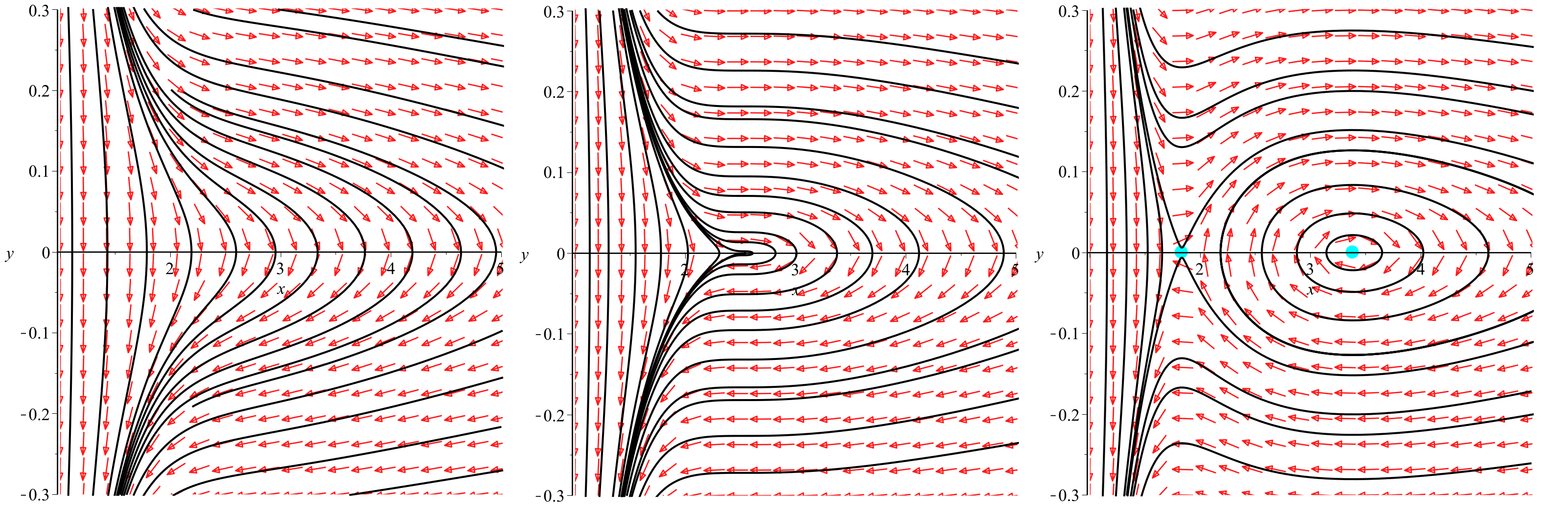
If the proper values of the Jacobian A associated with a system of differential equations, evaluated at the equilibrium point $x_0:=\left(x_0^1,x_0^2,\dots ,x_0^n\right)$, are known, with Equation (3), we obtain the behavior of solution near $x_0$. For example, if we consider a two-dimensional autonomous differential system, we obtain the following classification of the equilibrium points: if the eigenvalues of A have negative real parts, then in the phase plane, all solutions are converging towards the steady state (equilibrium point) $x_0$. The point $x_0$ is named a hyperbolic sink (stable point). Moreover, if the real parts of the proper values (eigenvalues) of A are greater then zero, then all integral curves diverge from the equilibrium point, and $x_0$ is named a hyperbolic source (unstable point). If one eigenvalue is positive, and the other one is negative, the fixed point $x_0$ is a saddle point (unstable). If the proper values (eigenvalues) of A are complex conjugate pairs, and $\mathrm{Re}\lambda \ne 0$, then the equilibrium point is a spiral point (stable if $\mathrm{Re}\lambda <0$, and unstable otherwise). If the proper values (eigenvalues) of A are purely imaginary values ($\mathrm{Re}\lambda =0$), the fixed point is named a center.

If the eigenvalues of the linearized system (2) evaluated in $x_0$ have nonzero real parts, then the equilibrium point is said to be hyperbolic. Otherwise, it is called nonhyperbolic. The relation between the linear stability of the system (1) and its linearization (2) at equilibrium points is given by the following Theorem.

Theorem 1

((Hartman–Grobman) [20]). Let us consider a system of ordinary differential equations $\dot{x}=f\left(x\right)$, $x\in R^n$, with the vector field f being $C^1$. Let us assume that $\overline{x}$ is a hyperbolic fixed point of the considered system of differential equations. Then, a neighborhood of the point $\overline{x}$, on which the flow is topologically equivalent to the flow of the linearization of the system of differential equations at $\overline{x}$, does always exist.

For the sake of completeness, we mention that the linear stability of the system (1) near a nonhyperbolic point could be investigated with the aid of the Lyapunov function introduced through the following Theorem and definition.

Theorem 2

((Lyapunov stability theorem) [20]). Let us consider that a vector field $\dot{x}=f\left(x\right)$, $x\in R^n$ is given. Let $\overline{x}$ denote an equilibrium point of the vector field $\dot{x}$. Moreover, let $\mathsf{\Sigma }:U\to R$ be a $C^1$ function, defined on some neighborhood U of $\overline{x}$, and having the properties

(i) $\mathsf{\Sigma }\left(\overline{x}\right)=0$ and $\mathsf{\Sigma }\left(x\right)>0$, if $x\ne \overline{x}$;

(ii) $\dot{\mathsf{\Sigma }}\left(x\right)\le 0$ in $U-\overline{x}$.

Then, if the conditions (i) and (ii) are satisfied, the point $\overline{x}$ is stable. Furthermore, if

(iii) $\dot{\mathsf{\Sigma }}\left(x\right)<0$ in $U-\overline{x}$, the point $\overline{x}$ is asymptotically stable.

The function $\mathsf{\Sigma }\left(x\right)$ from the above Theorem is called the Lyapunov function. It has the property that, near the equilibrium point $x_0$, the integral curves $f\left(x\right)$ are tangent to the surface levels of $\mathsf{\Sigma }$, or they cross the surface level oriented towards their interior. In other words, $\nabla \mathsf{\Sigma }\left(x_0\right)·f\left(x_0\right)\le 0$.

2.2. KCC Stability Theory

In the following, we introduce the basic ideas, and geometric concepts, of the KCC theory. Our presentation mostly follows the similar expositions of the theory in [8,25], respectively.

2.2.1. Geometrization of Arbitrary Dynamical Systems

We introduce first a set of dynamical variables $x^i$, $i=1,2,\dots ,n$, assumed to be defined on a real, smooth n-dimensional manifold $\mathcal{M}$. We denote in the following by $T\mathcal{M}$ the tangent bundle of $\mathcal{M}$. Usually, $\mathcal{M}$ is considered as $R^n$, $\mathcal{M}=R^n$, and therefore $T\mathcal{M}=T{R}^n=R^n$ [24].

Let us consider now a particular subset $\mathsf{\Omega }$ of the $(2n+1)$ dimensional Euclidian space defined as $R^n\times R^n\times R^1$. On $\mathsf{\Omega }$, we assume the existence of a $2n+1$ dimensional coordinate system denoted $\left(x^i,y^i,t\right)$, $i=1,2,\dots ,n$, where we have also introduced the notations $\left(x^i\right)=\left(x^1,x^2,\dots ,x^n\right)$, and $\left(y^i\right)=\left(y^1,y^2,\dots ,y^n\right)$, respectively. By t, we denote the ordinary time coordinate. We define the coordinates $y^i$ as

$$y^i=\left(\frac{d{x}^1}{dt},\frac{d{x}^2}{dt},\dots ,\frac{d{x}^n}{dt}\right).$$

(10)

A fundamental supposition in the KCC theory refers to the coordinate t, which can be interpreted physically as the time variable, and which is assumed to be an absolute invariant, which does not change in the coordinate transformations. Thus, by taking into account this assumption, on the base manifold $\mathcal{M}$, the only allowed transformations of the coordinates are of the general form [24],

$$\tilde{t}=t,{\tilde{x}}^i={\tilde{x}}^i\left(x^1,x^2,\dots ,x^n\right),i=1,2,\dots ,n.$$

(11)

In various mathematical applications of scientific importance, and interest, the equations of motion describing the evolution of natural or engineering systems are obtainable from a Lagrangian function L, which describes the state of the system, and is an application $L:T\mathcal{M}\to R$. The dynamical evolution of the system can be obtained with the help of the Euler–Lagrange equations, given by [24]

$$\frac{d}{dt}\frac{\partial L}{\partial y^i}-\frac{\partial L}{\partial x^i}=F_i,i=1,2,\dots ,n.$$

(12)

For the specific case of mechanical systems, the quantities $F_i$, $i=1,2,\dots ,n$ give the components of the external force $\overrightarrow{F}$, which cannot be derived from a potential. By assuming that the Lagrangian L is regular, by using some simple calculations, we obtain the fundamental results that the Euler–Lagrange equations Equation (12) are equivalent mathematically to a complicated system of second-order ordinary, strongly nonlinear differential equations, given by [8,24]

$$\frac{d^2{x}^i}{d{t}^2}+2G^i\left(x^j,y^j,t\right)=0,i=1,2,\dots ,n.$$

(13)

As for the functions $G^i$, we assume that each function $G^i\left(x^j,y^j,t\right)$ is $C^{\infty }$ in a neighborhood of some initial conditions $\left(x_0,y_0,t_0\right)$, defined in $\mathsf{\Omega }$.

The key conjecture of the KCC theory is the following. Let us assume that an arbitrary system of strongly nonlinear second-order ordinary differential equations of the form (13) is defined in a general form. Even if the Lagrangian function for the system is not known a priori, we still can investigate the evolution and the behavior of its trajectories by using techniques suggested by the differential geometry of the Finsler spaces. This analysis can be carried out due to the existence of a close similarity between the paths of the Euler–Lagrange system, and the geodesics in a Finsler geometry.

2.2.2. The Nonlinear and Berwald Connections, and the KCC Invariants Associated with a Dynamical System

To investigate from a geometrical perspective, the mathematical properties of the dynamical system described by the system of differential equations Equation (13), we first introduce the nonlinear connection N, defined on the base manifold $\mathcal{M}$, and having the coefficients $N_j^i$ given by [35]

$$N_j^i=\frac{\partial G^i}{\partial y^j}.$$

(14)

From a general geometric perspective, the nonlinear connection $N_j^i$ can be characterized with the help of a dynamical covariant derivative ${\nabla }^N$ by using the following procedure. Let us assume that two vector fields v and w, respectively, are given, with both vector fields defined over a manifold $\mathcal{M}$. Next, we define the covariant derivative ${\nabla }^N$ of w as [36]

$${\nabla }_v^{N}w=\left[v^l\frac{\partial }{\partial x^l}{w}^i+N_j^i(x,y)w^j\right]\frac{\partial }{\partial x^i}.$$

(15)

For $N_i^j(x,y)={\mathsf{\Gamma }}_{il}^j\left(x\right)v^l$, from Equation (15), we directly reobtain the definition of the standard covariant derivative for the particular case of the Levi–Civita linear connection, as introduced usually in the Riemannian geometry [36].

Now, we consider the open subset $\mathsf{\Omega }\subseteq R^n\times R^n\times R^1$ on which the system of differential Equation (13) is defined, together with the coordinate transformations, defined by Equation (11), and assumed to be non-singular. On this mathematical structure, we can define the KCC-covariant derivative of an arbitrary vector field ${\xi }^i\left(x\right)$ by means of the definition [9,10,11,12],

$$\frac{D{\xi }^i}{dt}=\frac{d{\xi }^i}{dt}+N_j^i{\xi }^j.$$

(16)

By taking ${\xi }^i=y^i$, we obtain

$$\frac{D{y}^i}{dt}=N_j^i{y}^j-2G^i=-{ϵ}^i.$$

(17)

The contravariant vector field ${ϵ}^i$ is defined on the subset $\mathsf{\Omega }$ of the Euclidian space, as one can see immediately from the above equation. It represents the first KCC invariant. From a general physical perspective, and within the mathematical formalism of the classical Newtonian mechanics, ${ϵ}^i$, the first KCC invariant, could be understood as an external force, not derivable from a potential, and acting on the dynamical system.

As a next step in our discussion of the KCC theory, we consider the infinitesimal variations of the trajectories $x^i\left(t\right)$ of the dynamical system (13) into neighbouring ones, with the variations defined according to the prescriptions,

$${\tilde{x}}^i\left(t\right)=x^i\left(t\right)+\eta {\xi }^i\left(t\right),{\tilde{y}}^i\left(t\right)=y^i\left(t\right)+\eta \frac{d{\xi }^i\left(t\right)}{dt},$$

(18)

where, by $\left|\eta \right|<<1$, we have denoted a small infinitesimal quantity, while ${\xi }^i\left(t\right)$ denotes the components of an arbitrary contravariant vector field $\xi$. The vector field $\xi$ is defined along the trajectory $x^i\left(t\right)$ of the system of the differential equations under consideration. After the substitution of Equation (18) into Equation (13), and by considering the limit $\eta \to 0$, we arrive to the deviation, or Jacobi, equations, representing the central mathematical result of the KCC theory, and which are given by [9,10,11,12]

$$\frac{d^2{\xi }^i}{d{t}^2}+2N_j^i\frac{d{\xi }^j}{dt}+2\frac{\partial G^i}{\partial x^j}{\xi }^j=0.$$

(19)

With the help of the KCC-covariant derivative, as introduced in Equation (16), we can reformulate Equation (19) in a fully covariant form as

$$\frac{D^2{\xi }^i}{d{t}^2}=P_j^i{\xi }^j,$$

(20)

where we have denoted

$$P_j^i=-2\frac{\partial G^i}{\partial x^j}-2G^l{G}_{jl}^i+y^l\frac{\partial N_j^i}{\partial x^l}+N_l^i{N}_j^l+\frac{\partial N_j^i}{\partial t}.$$

(21)

In Equation (21), we have defined the important tensor $G_{jl}^i$, given by [8,9,10,11,12,35]

$$G_{jl}^i\equiv \frac{\partial N_j^i}{\partial y^l},$$

(22)

and which in the KCC theory is named the Berwald connection.

The tensor $P_j^i$ is called the second KCC-invariant. It is the fundamental quantity in the KCC theory, and in the Jacobi stability investigations. Alternatively, $P_j^i$ is also called the deviation curvature tensor, by indicating its essential geometric nature. Furthermore, we will call in the following Equation (20) the Jacobi equation. This equation exists in both Riemann or Finsler geometries. If one assumes that the system of Equation (13) corresponds to the geodesic motion of a physical system, then Equation (20) gives the so-called Jacobi field equation, which can always be introduced in the considered geometry.

The trace $P=P_i^i$ of the curvature deviation tensor, constructed from $P_j^i$, is a scalar invariant. It can be calculated from the relation

$$P=P_i^i=-2\frac{\partial G^i}{\partial x^i}-2G^l{G}_{il}^i+y^l\frac{\partial N_i^i}{\partial x^l}+N_l^i{N}_i^l+\frac{\partial N_i^i}{\partial t}.$$

(23)

Other important invariants can also be constructed in the KCC theory. The most commonly used invariants are the third, fourth and fifth invariants associated with the given dynamical system, whose evolution and behavior is represented by the second order system of nonlinear Equation (13). These invariants are introduced according to the definitions [9]

$$P_{jk}^i\equiv \frac{1}{3}\left(\frac{\partial P_j^i}{\partial y^k}-\frac{\partial P_k^i}{\partial y^j}\right),P_{jkl}^i\equiv \frac{\partial P_{jk}^i}{\partial y^l},D_{jkl}^i\equiv \frac{\partial G_{jk}^i}{\partial y^l}.$$

(24)

From a geometrical perspective, $P_{jk}^i$, the third KCC invariant, can be described as a torsion tensor. $P_{jkl}^i$, the fourth KCC invariant, represents the equivalent of the Riemann–Christoffel curvature tensor, while $D_{jkl}^i$, the fifth KCC invariant, is called the Douglas tensor [8,9]. Let us point out now that, in a Berwald geometry, these three tensors can always be defined. It is also important to mention that, in the KCC theory, the five invariants defined above are the fundamental mathematical quantities that describe the geometrical properties, and interpretation, of a dynamical system whose time evolution and behavior are represented by an arbitrary system of second-order strongly nonlinear differential equations.

2.2.3. Jacobi Stability of Dynamical Systems

In a large number of scientific investigations, the analysis of the stability of biological, chemical, biochemical, engineering, medical or physical systems, as well as the study of the trajectories of a system of differential equations, as given, for example, by Equation (13), in the vicinity of a given point $x^i\left(t_0\right)$, is of fundamental significance for the understanding of its properties. Moreover, the study of the stability can give important information on the temporal evolution of a general dynamical system.

For simplicity, in the following, we adopt as the origin of the time variable t the value $t_0=0$. Moreover, we define $〈.,.〉$ as representing the canonical inner product of $R^n$. We also introduce the null vector O defined in $R^n$, $O\in R^n$. Next, we assume that the trajectories $x^i=x^i\left(t\right)$ of the system of differential Equation (13) represent smooth curves in the Euclidean space $R^n$, endowed with the canonical inner product $〈.,.〉$. Moreover, to completely characterize the deviation vector $\xi$, we assume, as a general property, that it satisfies the set of two essential initial conditions $\xi \left(0\right)=O$ and $\dot{\xi }\left(0\right)=W\ne O$, respectively [8,9,10,11].

To describe the dispersing/focusing trend of the trajectories of a dynamical system around $t_0=0$, we introduce the following intuitive and simple mathematical picture. Let us assume first that the deviation vector $\xi$ satisfies the condition $\left|\left|\xi \left(t\right)\right|\right|<t^2$, $t\approx 0^{+}$ [8,24]. If this is the case, then it turns out that all the trajectories of the dynamical system are focusing together, and converge towards the origin. Let us assume now that the deviation vector $\xi$ has the property that the condition $\left|\left|\xi \left(t\right)\right|\right|>t^2$, $t\approx 0^{+}$ is satisfied. In this case, it follows that all the solutions of the system of differential Equation (13) have at infinity a dispersing behavior [8,9,10,11].

The dispersing/focusing behavior of the solutions of a given system of second order ordinary differential equations can be also characterized, from the geometrical perspective introduced by the KCC theory, by considering the algebraic properties of the deviation curvature tensor $P_i^j$. This can be achieved in the following way. For $t\approx 0^{+}$, the trajectories of the system of strongly nonlinear equations Equation (13) are bunching/focusing together if and only if the real parts of the characteristic values (eigenvalues) of the deviation tensor $P_j^i\left(0\right)$ are strictly negative. Otherwise, the trajectories of the dynamical system have a dispersing behavior if and only if the real parts of the characteristic values (eigenvalues) of $P_j^i\left(0\right)$ are strictly positive [8,9,10,11].

By taking into account the qualitative discussion presented above, we present now the rigorous mathematical definition of the notion of Jacobi stability for an arbitrary dynamical system, described by a system of ordinary second order differential equations, which is given by the following [8,9,10,11]:

Definition 2.

Let us consider that the general system of differential equations Equation (13), describing the time evolution of a dynamical system, satisfies the initial conditions:

$$\left|\right|x^i\left(t_0\right)-{\tilde{x}}^i\left(t_0\right)\left|\right|=0,\left|\right|{\dot{x}}^i\left(t_0\right)-{\dot{\tilde{x}}}^i\left(t_0\right)\left|\right|\ne 0,$$

defined with respect to the norm$\left|\left|.\right|\right|$induced by a positive definite inner product.

If these conditions are satisfied, the trajectories of the dynamical system, given by Equation (13), are designated as Jacobi stable if and only if the real parts of the characteristic values (eigenvalues) of the curvature deviation tensor $P_j^i$ are everywhere strictly negative.

On the other hand, if the real parts of the characteristic values (eigenvalues) of the curvature deviation tensor $P_j^i$ are strictly positive everywhere, the trajectories of the dynamical system are designated as unstable in the Jacobi sense.

This definition allows us to straightforwardly investigate the stability of the systems of second order differential equations, and of the associated dynamical systems, as an alternative to the standard Lyapunov linear stability method.

2.3. The Correlation between Lyapunov and Jacobi Stability for a Two-Dimensional Autonomous Differential System

Let us recall that the Lyapunov stability is determined by the nature and sign of the eigenvalues of the Jacobian matrix evaluated at an equilibrium point (fixed point). On the other hand, the Jacobi stability is given by the sign of the real part of the eigenvalues of the curvature deviation tensor $P_j^i$, calculated at the same point.

The Jacobi stability of the two-dimensional systems of first order differential equations was explored in [10,11], where the authors considered a system of two arbitrary differential equations written in the general form,

$$\frac{du}{dt}=f(u,v),\frac{dv}{dt}=g(u,v).$$

(25)

Moreover, it was assumed that the point $(0,0)$ is a fixed point of the system (25), that is, $f(0,0)=g(0,0)=0$. If the equilibrium point is $(u_0,v_0)\ne (0,0)$, with the change of the variable $\tilde{u}=u-u_0$, and $\tilde{v}=v-v_0$, respectively, the equilibrium point $(u_0,v_0)$ is moved to the origin $(0,0)$.

In the approach pioneered in [10,11], after relabelling the variables by denoting v as x, and $g(u,v)$ as y, and by also assuming that the condition $g_u{|}_{(0,0)}\ne 0$ is satisfied by the function $g(u,v)$, it turns out that it is possible to eliminate from the system of the two equations (25) the variable u. By taking into account that the point $(u,v)=(0,0)$ is a fixed point, from the Theorem of the Implicit Functions, it follows that, in the neighbourhood of the point $(x,y)=(0,0)$, the algebraic equation $g(u,x)-y=0$ has a unique solution $u=u(x,y)$. By taking into account that $\ddot{x}=\dot{g}=g_{u}f+g_{v}y$, where the subscripts denote the partial derivatives with respect to u and v, respectively, one obtains finally an autonomous one-dimensional second order equation, equivalent mathematically to the system (25), and which is obtained in the general form as

$${\ddot{x}}^1+g^1(x,y)=0,$$

(26)

where

$$g^1(x,y)=-g_u(u(x,y),x)f(u(x,y),x)-g_v(u(x,y),x)y.$$

(27)

Hence, the Jacobi stability properties of a system of two arbitrary first order differential equations can be studied in detail via the equivalent Equation (26) by using the methods of the KCC theory [10,11]. Thereupon, the KCC stability properties of a first order system of differential equations of the form (25) can also be determined easily, thus allowing an in depth comparison between the Jacobi and Lyapunov stability properties of the two-dimensional dynamical systems, which can be performed in a straightforward manner [8].

Let us recall some results from [8] which are applied in this paper. The Jacobian matrix of (25) is

$$J(u,v)=\left(\begin{array}{cc}{f}_u& f_v\\ g_u& g_v\end{array}\right).$$

(28)

The characteristic equation is given by

$${\lambda }^2-\left(\mathrm{tr}A\right)\lambda +detA=0,$$

(29)

where $\mathrm{tr}A=f_u+g_v$, and $detA=f_u{g}_v-g_u{f}_v$ are the trace and the determinant of the Jacobian matrix ${A=J|}_{(0,0)}$, respectively.

The signs of the discriminant $\Delta ={(f_u-g_v)}^2+4f_v{g}_u$, and the trace and the determinant of A, give the Lyapunov (linear) stability of the fixed point $(0,0)$.

The system (25) is equivalent from a mathematical point of view to the second order differential Equation (26). Performing the Jacobi stability analysis for this last equation in [8], assuming that $g_u{|}_{(0,0)}\ne 0$, the authors obtained the result that the curvature deviation tensor $P_1^1$ at the fixed point $(0,0)$ is given by

$$4P_1^1{|}_{(0,0)}=-4g_{,1}^1{{|}_{(0,0)}+{(g_{;1}^1)}^2|}_{(0,0)}=\Delta ,$$

(30)

where

$$\Delta :={\left(trA\right)}^2-4detA$$

is the discriminant of the characteristic Equation (29) and ${A=J|}_{(0,0)}$. Therefore, the authors of [8] concluded their analysis by formulating the following

Theorem 3

([8]). Let us consider the system of two first order ordinary differential equations, given by Equation (25), with the fixed point $P(0,0)$, such that $g_u|(0,0)\ne 0$. Then, the trajectory $v=v\left(t\right)$ is Jacobi stable if and only if $\Delta <0$.

Boehmer et al. [8] emphasized also that, if $f_v{|}_{(0,0)}\ne 0$, eliminating the variable v and relabeling u as x, we obtain a similar result that the trajectory $u=u\left(t\right)$ is Jacobi stable if and only if $\Delta <0$.

In other words, they demonstrated that: if one considers the system of ordinary differential Equation (25) with the fixed point $P(0,0)$ located in the origin of the coordinate system, and satisfying the condition $g_u|(0,0)\ne 0$, then the Jacobian matrix J evaluated at the point P has complex proper values (eigenvalues) if and only if P satisfies the condition of being a stable point in the Jacobi sense.

Let us recall that the condition of stability in the Lyapunov sense for a solution of the dynamical system (25) is that $\mathrm{Re}\lambda <0$ for all roots of the characteristic (eigenvalue) Equation (29). The condition for the Jacobi stability thus requires that the discriminant of the same characteristic (eigenvalue) equation to take negative values. Consequently, Lyapunov stability is in general not equivalent with Jacobi stability, and it is worth finding out the equilibrium points where a system is stable in both Jacobi and Lyapunov sense.

In the next section, we will investigate the relation between Jacobi and Lyapunov stability of the circular orbits around a GMGHS black hole.

3. Black Hole Solutions in Dilaton Gravity

Theoretical models based on the field equations obtained from the string-like action [28,29]

$$S=-\frac{1}{2}\int d^{4}x\sqrt{-g}\left[R-2\gamma {\left(\nabla \varphi \right)}^2+e^{-2\alpha \varphi }{F}^2\right],$$

(31)

where $\alpha =\mathrm{constant}>0$, and $\gamma =\mathrm{constant}>0$, have been extensively investigated in the physical literature. In Equation (31), $\varphi$ denotes the dilaton field, while F represents the Maxwell two-form field, having the components defined as $F_{\mu \nu }={\partial }_{\mu }{A}_{\nu }-{\partial }_{\nu }{A}_{\mu }$. The action (31) can be obtained from the string frame low energy effective action, given by

$$\widehat{S}=-\int d^{4}x\sqrt{-\widehat{g}}{e}^{-2\alpha \varphi }\left[\widehat{R}-2\gamma {\left(\widehat{\nabla }\varphi \right)}^2+F^2\right],$$

(32)

by using the conformal transformation ${\widehat{g}}_{\mu \nu }=e^{2\alpha \varphi }{g}_{\mu \nu }$. As particular cases, the models constructed from the action (32) include the Einstein–Maxwell theory, corresponding to $\alpha =\gamma =0$, and low energy string theory, which is obtained by taking $\alpha =2$, and $\gamma =2$, respectively.

The gravitational field equations derived from the action (32) by varying the metric are given by [29]

$${\nabla }_{\mu }\left(e^{-2\varphi }{F}^{\mu \nu }\right)=0,{\nabla }^2\varphi +\frac{1}{2}{e}^{-2\varphi }{F}^2=0,$$

(33)

and

$$R_{\mu \nu }=2{\nabla }_{\mu }\varphi {\nabla }_{\nu }\varphi +2e^{-2\varphi }{F}_{\mu \rho }{F}_{\nu }^{\rho }-\frac{1}{2}{g}_{\mu \nu }{e}^{-2\varphi }{F}^2,$$

(34)

respectively. By assuming for the static, spherically symmetric metric an ansatz of the form,

$$d{s}^2=-{\lambda }^{2}d{t}^2+\frac{d{r}^2}{{\lambda }^2}+R^{2}d\mathsf{\Omega },$$

(35)

where $\lambda$ and R are functions of r only, Gibbons and Maeda [28], and, independently, three years later, Garfinkle, Horowitz and Strominger [29] found that the unique static charged black hole solution corresponding to the action (31) is given by

$$d{s}^2=-\left(1-\frac{2M}{r}\right)d{t}^2+\frac{1}{\left(1-\frac{2M}{r}\right)}d{r}^2+r\left(r-\frac{Q^2}{M}\right)(d{\theta }^2+{sin}^2\theta d{\phi }^2)$$

(36)

where the electric field strength, and the dilaton field is given by

$$F_{rt}=\frac{Q}{r^2},e^{2\alpha \varphi }=1-\frac{Q^2}{Mr}.$$

(37)

This form of the metric is different from the usual standard form of a spherically symmetric metric, like, for example, the Schwarzschild metric. The above black hole solution (36) is known as a GMGHS black hole. For $Q^2<2M^2$, the black hole has an event horizon, and if $Q^2=2M^2$, the solution corresponds, from a physical point of view, to a naked singularity. This later case is called the extremal GMGHS black hole solution.

An external observer cannot see the region inside the event horizons. The main physical characteristics of a black hole can be acquired by investigating the behavior of matter and light outside the event horizons. A massive test particle moves along time-like geodesics, and photons move on null geodesics. The geodesics of a GMGHS black hole were studied extensively, for both the extremal and the non-extremal cases [37,38,39,40,41,42]. In what follows, we will consider the Jacobi stability of circular time-like geodesics around a GMGHS black hole. The existence and the Lyapunov stability of the circular orbits around GMGHS black holes was already investigated in [41].

Geodesic Equations in a Static-Charged Black Hole Geometry

We derive now the geodesics equations in the GMGHS space-time by using the mathematical formalism based on the Euler–Lagrange Equation (12). The Lagrangian for the metric (36) is:

$$2\mathcal{L}=-\left(1-\frac{2M}{r}\right){\dot{t}}^2+\frac{{\dot{r}}^2}{\left(1-\frac{2M}{r}\right)}+r\left(r-\frac{Q^2}{M}\right)\left({\dot{\theta }}^2+{sin}^2\theta {\dot{\phi }}^2\right)$$

(38)

where by a dot we have denoted the differentiation with respect to $\tau$—an affine parameter defined along the geodesic line. The parameter $\tau$ is chosen so that the Lagrangian $\mathcal{L}$ satisfies the condition $2\mathcal{L}=-1$ on a time-like geodesics, $2\mathcal{L}=0$ on a null geodesics, and $2\mathcal{L}=1$ on a space-like geodesics, respectively. Moreover, all the functions $F_i$, $i=1,2,\dots n$, from the right-hand side of Equation (12) are zero.

We recall that the coordinates t and $\phi$ are cyclic. Thus, we obtain that

$$\left(1-\frac{2M}{r}\right)\dot{t}=\mathrm{constant}=E,$$

(39)

is the energy integral, where E is the total energy of the particle, and

$$2{sin}^2\theta ·r\left(1-\frac{2M}{r}\right)\dot{\phi }=\mathrm{constant}=L,$$

(40)

is the integral of the angular momentum.

The Euler–Lagrange equation for $\theta$ is

$$\frac{d}{d\tau }\left[r\left(r-\frac{Q^2}{M}\right)\dot{\theta }\right]=r\left(r-\frac{Q^2}{M}\right)sin\theta cos\theta ·{\dot{\phi }}^2.$$

(41)

We note that, if $\theta =\pi /2$, then $\dot{\theta }\equiv 0$, $\ddot{\theta }\equiv 0$, and therefore $\theta =\pi /2$ is located on the geodesic curve. Thus, the motion of a massive particle is planar. On the other hand, the angular momentum integral (40) takes the form,

$$r\left(1-\frac{2M}{r}\right)\dot{\phi }=L,$$

(42)

where L represents, from a physical point of view, the angular momentum of the particle, oriented in the direction of an axis perpendicular to the plane in which the motion of the particle takes place.

Being complicated, the Euler–Lagrange equation for r is replaced with the constancy of the Lagrangian,

$$\frac{1}{2}{\left(\frac{dr}{d\tau }\right)}^2+\frac{1}{2}\left(1-\frac{2M}{r}\right)\left[\frac{L^2}{r\left(r-\frac{Q^2}{M}\right)}-ϵ\right]=E^2,$$

(43)

where the constant $ϵ$ takes the numerical values $ϵ=-1$ for time-like geodesics, $ϵ=0$ for null geodesics, and $ϵ=+1$ for space-like geodesics, respectively. The second term on the left-hand side of Equation (43) is the effective potential. Hence, Equation (43) can be written as

$$\frac{1}{2}{\left(\frac{dr}{d\tau }\right)}^2+V\left(r\right)=E^2$$

(44)

A massive test particle moving freely around a GMGHS black hole describes a time-like geodesic line. For them $ϵ=-1$, and the effective potential, becomes

$$V\left(r\right)=\frac{1}{2}\left(1-\frac{2M}{r}\right)\left[\frac{L^2}{r\left(r-\frac{Q^2}{M}\right)}+1\right].$$

(45)

By introducing the new variable $\eta$, defined as $r=2M\eta$, the effective potential (45) becomes

$$V\left(\eta \right)=\frac{1}{2}\left(1-\frac{1}{\eta }\right)\left[\frac{l^2}{{\eta }^2\left(1-\frac{q^2}{\eta }\right)}+1\right],$$

(46)

where we have denoted $l^2=L^2/4M^2$, and $q^2=Q^2/2M^2$, respectively. The variation of the potential $V\left(\eta \right)$ is presented, for different values of l and q, in Figure 1.

The first derivative of the potential can be obtained immediately as

$$V^{\prime }\left(\eta \right)=\frac{1}{2{\eta }^2}\left[1+\frac{l^2}{{\eta }^2}\frac{(1-\frac{2}{\eta })q^2-2(1-\frac{3}{2\eta })\eta }{{\left(1-\frac{q^2}{\eta }\right)}^2}\right].$$

(47)

The variation of the derivative $V^{\prime }\left(\eta \right)$ of the potential as a function of $\eta$ is represented in Figure 2.

For the second derivative of the potential, we obtain

$$V^{″}\left(\eta \right)=-\frac{2}{{\eta }^3}\left[1-\frac{l^2}{{\eta }^4}\frac{3(1-\frac{2}{\eta }){\eta }^2+(1-\frac{3}{\eta })q^4-3(1-\frac{8}{3\eta })\eta q^2}{{\left(1-\frac{q^2}{\eta }\right)}^3}\right].$$

(48)

The variation of $V^{″}\left(\eta \right)$ is presented, for different values of l and q, in Figure 3.

The dependence of the real solution ${\eta }_0$ of the equation $V^{\prime }\left({\eta }_0\right)=0$ on the parameters $l^2$ and $q^2$ of the GMGHS black hole solution is represented in Figure 4.

4. Stability of the Circular Orbits of the Free Test Particles in a GMGHS Spacetime

Next, we will consider the stability in Lyapunov and Jacobi sense of the circular orbits on which massive test particles move freely around a GMGHS black hole.

4.1. Lyapunov Stability Analysis

Equation (43) is the starting point in the dynamical systems approach for the analysis of the stability of the geodesic curves in the GMGHS geometry. Differentiating Equation (43) with respect to $\tau$ and dividing the result with $\dot{r}$, we obtain the following second order differential equation

$$\ddot{r}=-\frac{dV}{dr}.$$

(49)

Equation (49) corresponds to following system of first order differential equations:

$$\frac{dr}{d\tau }=p\frac{dp}{d\tau }=-\frac{dV}{dr}.$$

(50)

The Jacobian matrix of the system (50) is

$$J=\left(\begin{array}{cc}0& 1\\ -V^{″}\left(r\right)& 0\end{array}\right)$$

(51)

where ${}^{\prime }$ means differentiation with respect to r.

The characteristic equation is

$${\lambda }^2+V^{″}\left(r\right)=0,$$

(52)

and the proper values (eigenvalues) of the Jacobian matrix associated with the system (50) are given by

$$\lambda =\pm \sqrt{-V^{″}\left(r\right)},$$

(53)

and so a simple fixed point $(r_0,0)$ of (50) is a saddle point if $(V^{″}\left(r_0\right)<0)$ and a center if $(V^{″}\left(r_0\right)>0)$.

In [41], the existence and stability in the sense of Liapunov of circular time-like geodesics around a GMGHS black hole were explored. The study showed that, for certain values of the parameters, outside the black hole, there are two circular geodesics. In other words, outside the black hole, we can find two values $r_0>2M$ so that $V^{\prime }\left(r_0\right)=0$, one for a minimum of the effective potential ($V^{″}\left(r_0\right)<0$) and the other for a maximum of the potential ($V^{″}\left(r_0\right)>0$).

If $V^{″}\left(r_0\right)<0$, the eigenvalues (53) of the linearization of the system (50) are real and have opposite signs; therefore, the fixed point $(r_0,0)$ of the system is a saddle point, which is Liapunov unstable. A saddle point is a hyperbolic point, and so, based on the Hartman–Grobman theorem, the fixed point $(r_0,0)$ of the system (50) is Liapunov unstable.

If $V^{″}\left(r_0\right)>0$, the values of $\lambda$ from (53) are purely complex conjugate, and the study of the linear stability of system at the fixed point $(r_0,0)$ begins with the search of a Liapunov function for the system (50). We note that the function

$$\mathbf{V}(r,p)=\frac{p^2}{2}+V\left(r\right)$$

(54)

has the property that $\nabla \mathbf{V}(r,p)·f(r,p)=0,\forall (r,p)$, where $f(r,p)=\left(p,-dV/dr\right)$, meaning that the function (54) could be chosen as a Liapunov function. Furthermore, we have to check if $\mathbf{V}$ fulfills the condition of the Liapunov stability theorem. In other words, we have to verify if the fixed point is a local minimum of $\mathbf{V}$. Therefore, we compute the Hessian matrix of $\mathbf{V}$

$${\mathcal{H}}_{\mathbf{V}}=\left(\begin{array}{cc}{V}^{″}\left(r\right)& 0\\ 0& 1\end{array}\right).$$

(55)

We note that the matrix (55) is positive definite when $V^{″}\left(r\right)>0$, meaning that the fixed point $(r_0,0)$ of the linearized system corresponding to (50) is a center. In addition, thus, we finally conclude that the circular orbits around a GMGHS black hole, $r=r_0=\mathrm{constant}$, are Lyapunov stable when $V^{″}\left(r_0\right)>0$, and Lyapunov unstable when $V^{″}\left(r_0\right)<0$.

4.2. Jacobi Stability Analysis

In this section, we will first perform the study of the Jacobi stability analysis of Equation (49), giving the geodesic trajectories of a massive particle in the GMGHS geometry. Then, we will consider the stability of the circular orbits in both Lyapunov and KCC approaches.

4.2.1. Stability of the GMGHS Orbits in the General Case

The affine parameter $\tau$ in the geodesic Equation (49) is an absolute invariant, and hence all the results of the KCC theory can be applied to this case. By introducing the dimensionless radial coordinate $\eta$, the geodesic equation of motion in the GMGHS geometry takes the form

$$\frac{d^2\eta \left(\tau \right)}{d{\tau }^2}+\frac{1}{4M^2}\frac{dV\left(\eta \right)}{d\eta }=0,$$

(56)

or, equivalently,

$$\begin{array}{ccc}& & \frac{d^2\eta \left(\tau \right)}{d{\tau }^2}+\frac{1}{4M^2}\{\frac{1}{{\eta }^2\left(\tau \right)}\left[1+\frac{l^2}{{\eta }^2\left(\tau \right)\left(1-\frac{q^2}{\eta \left(\tau \right)}\right)}\right]\hfill \\ & & -\left(1-\frac{1}{\eta \left(\tau \right)}\right)\left[\frac{2l^2}{{\eta }^3\left(\tau \right)\left(1-\frac{q^2}{\eta \left(\tau \right)}\right)}+\frac{l^2{q}^2}{{\eta }^4\left(\tau \right){\left(1-\frac{q^2}{\eta \left(\tau \right)}\right)}^2}\right]\}=0.\hfill \end{array}$$

(57)

By denoting $\eta \left(\tau \right)=x^1$, and ${\eta }^{\prime }\left(\tau \right)=y^1$, Equation (56) takes the form

$$\frac{d^2{x}^1}{d{\tau }^2}+2G^1\left(x^1\right)=0,$$

(58)

where

$$G^1\left(x^1\right)=\frac{1}{8M^2}\frac{dV\left(x^1\right)}{d{x}^1},$$

(59)

or

$$\begin{array}{ccc}& & G^1\left(x^1\right)=\frac{1}{8M^2}\{\frac{1}{{\left(x^1\right)}^2}\left[1+\frac{l^2}{{\left(x^1\right)}^2\left(1-\frac{q^2}{x^1}\right)}\right]\hfill \\ & & \left(1-\frac{1}{x^1}\right)\left[\frac{2l^2}{{\left(x^1\right)}^2\left(1-\frac{q^2}{x^1}\right)}+\frac{l^2{q}^2}{{\left(x^1\right)}^2{\left(1-\frac{q^2}{x^1}\right)}^2}\right]\}.\hfill \end{array}$$

(60)

The nonlinear connection associated with Equation (58) is obtained as

$$N_1^1=\frac{\partial G^1\left(x^1\right)}{\partial y^1}\equiv 0.$$

(61)

For the Berwald connection, we have

$$G_{11}^1=\frac{\partial N_1^1}{\partial y^1}\equiv 0.$$

(62)

For the curvature deviation tensor, we obtain now the simple expression

$$P_1^1=-2\frac{\partial G^1\left(x^1\right)}{\partial x^1}=-\frac{1}{4M^2}{V}^{″}(x^1)).$$

(63)

Hence, the geodesic trajectories of a massive test particle in the spherically symmetric GMGHS black hole are Jacobi stable if the condition $-\left.V^{″}\left(x^1\right)\right|x^1=x_0^1<0$. On the other hand, we obtain a geometric interpretation of the second derivative of the potential, giving the deviation curvature tensor of the geodesic trajectories. On the other hand, for the first KCC invariant of the system, we obtain

$${ϵ}^1=2G^1\left(x^1\right)=\frac{1}{4M^2}\frac{dV\left(x^1\right).}{d{x}^1}$$

(64)

Hence, the first derivative of the potential, representing physically the force acting on the particle, has a geometric interpretation as the first KCC invariant. Moreover, the geodesic deviation equations take the form

$$\frac{d^2{\xi }^1}{d{\tau }^2}+\frac{1}{4M^2}{V}^{″}\left(x^1\right){\xi }^1=0.$$

(65)

The variation of the deviation curvature tensor of the GMGHS black hole is represented as a function of the solution parameters l and q, for a fixed value of $\eta$, in Figure 5. The contour plot of the deviation tensor is also represented.

4.2.2. Stability of the Circular Orbits

In this section, we will perform the Jacobi stability of the system (50) using the results obtained by Boehmer et al. in [8]. For the system (50), we consider the Jacobian matrix of the system and evaluate its trace and determinant

$$\mathrm{tr}J=0detJ=V^{″}\left(r\right).$$

(66)

Thus, the discriminant of the characteristic equation becomes

$$\Delta =\mathrm{tr}{\left(J\right)}^2-4\det \left(J\right)=-4V^{″}\left(r\right).$$

(67)

Based on the Theorem which makes the link between the discriminant of the characteristic equation and the Jacobi stability, we can conclude that the circular orbit of a free particle moving in an GMGHS spacetime, $r=r_0$, is Jacobi stable when $V^{″}\left(r_0\right)>0$ and Jacobi unstable for $V^{″}\left(r_0\right)<0$.

We note that we have found the same condition for Jacobi stability as for the for Lyapunov stability, meaning that, for the circular orbits on which massive test particle move around a GMGHS black hole, the two types of stability coincide.

We consider now some particular cases of stability, corresponding to some specific values of the parameters l and q of the GMGHS black hole. By taking $l=8$, and $q=0.95$, it turns out that the equation $V^{\prime }\left(\eta \right)=0$ has two real solutions satisfying the condition $\eta >1$, given by ${\eta }_1=1.1996$ and ${\eta }_2=127.8522$. Evaluating the second derivative of the potential in these points gives ${\left.V^{″}\left(\eta \right)\right|}_{\eta =1.19996}=-185.5041<0$, and ${\left.V^{″}\left(\eta \right)\right|}_{\eta =127.8522}=+2.39\times {10}^{-7}>0$, respectively. Hence, we can conclude that the circular trajectory located at $r=2M{\eta }_1$ is both Lyapunov and Jacobi unstable (left panel in Figure 6), while the circular trajectory located at $r=2M{\eta }_2$ is both Lyapunov and Jacobi stable (right panel in Figure 6).

Let us now consider the Lyapunov stability corresponding to the value $l=3/2$ of the parameter l of a GMGHS black hole. By taking $q\in \{0.55,0.6512,0.75\}$, the equation $V^{\prime }\left(\eta \right)=0$ has no real solution, two real and equal solutions, and two different real solutions, satisfying the condition $\eta >1$, meaning that, outside the black hole, there are no circular orbits, one circular orbit and two circular orbits, respectively. For $q=0.6512$, ${\eta }_1=$${\eta }_2=2.5243$, by evaluating the second derivative of the potential, we obtain ${\left.V^{″}\left(\eta \right)\right|}_{\eta =2.5243}=0$, the point $\eta =2.5243$ is an inflection point for the potential, which leads to a cusp in the phase diagram (see the middle panel in Figure 7). For $q=0.75$, ${\eta }_1=1.8333$ and ${\eta }_2=3.3836$ and by evaluating the second derivative of the potential in these points, we obtain ${\left.V^{″}\left(\eta \right)\right|}_{\eta =1.8333}=-0.111<0$ and ${\left.V^{″}\left(\eta \right)\right|}_{\eta =3.3836}=+0.0075>0$, respectively. Therefore, we can conclude that the circular trajectory located at $r=2M{\eta }_1$ is Lyapunov unstable, and the circular trajectory located at $r=2M{\eta }_2$ is Lyapunov stable (see the right panel in Figure 7).

5. Conclusions

In the present paper, we have first revisited, and carefully investigated, two methods of stability analysis: Lyapunov stability and the Jacobi stability approaches, respectively. The Lyapunov stability analysis is conducted by the linearization of the system of differential equations describing the dynamical system at the fixed points. On the other hand, and Jacobi stability involves the perturbations of a whole set of trajectories. Intuitively, the Jacobi stability indicates how the trajectories bunch together, or disperse, when approaching the fixed point.

As an application of the two stability methods, we have comparatively investigated the behavior of the trajectories of the solutions for a specific charged black hole solution that originates in the low energy limit of string theory, called the GMGHS solution. The study of the properties of the geodesic curves in black hole geometries is an important field of investigation [37,38,39,40,41,42], which could lead not only to a better understanding of the theoretical properties of these objects, but could also open new perspectives on their observational detection. Moreover, black holes represent a fertile testing ground of modified gravity theories.

An analysis of the stability of the orbits in the Schwarzschild geometry was performed in [20], by using both Lyapunov and Jacobi stability approaches. As a result of this study, it was shown that stable circular orbits do exist at a radius $r_{\ast }=R_{+}$, where $R_{+}=\left(L^2+\sqrt{L^4-12L^2{M}^2}\right)/2M$, while unstable circular orbits exist at $r_{\ast }=R_{-}$, where $R_{-}=\left(L^2-\sqrt{L^4-12L^2{M}^2}\right)/2M$. A similar analysis of the motion of the particles in Newtonian mechanics in the presence of a central force field $f\left(r\right)$ was carried out in [19]. In nonrelativistic mechanics, circular orbits in a central field do exist if the equation

$$V^{\prime }\left(r\right)=-f\left(r\right)-\frac{L^2}{M{r}^3}=0,$$

(68)

has real roots. Furthermore, if $r=r_0$ is a root of $V^{\prime }\left(r\right)=0$, the circular orbit is stable if the condition

$${\left.V^{″}\left(r\right)\right|}_{r=r_0}=-{\left.f^{\prime }\left(r\right)\right|}_{r=r_0}+\frac{3L^2}{M{r}_0^4}>0,$$

(69)

is satisfied.

In a realistic astrophysical environment, massive general relativistic objects, like, for example, black holes or neutron stars, are often enclosed by an accretion disk. Accretion disks around compact objects can be the basis of physical models that could convincingly provide explanations for many astrophysical phenomena, like, for example, active galactic nuclei and X-ray binaries. The disks can be described theoretically by assuming that they are composed of massive test particles (baryons) that evolve in the gravitational field of the central massive and compact astrophysical object. The disks cool down through the electromagnetic radiation emission from their surface, and this form of energy emission represents an efficient physical mechanism for avoiding the extreme heating of the disk surface [43]. The disk has an inner edge, which is located at the marginally stable orbits of the gravitational, potential created by the central massive compact object. Hence, in higher orbits, the motion of the gas in the disk is Keplerian.

Therefore, the problem of the determination of the position of circular orbits, and of their stability, is fundamental from an astrophysical point of view. The electromagnetic emissivity properties of the accretion disks provide distinct observational signatures for different classes of astrophysical objects, including black holes, neutron, quark or other types of exotic stars. The parameters l and q of the GMGHS black hole can also be constrained from the physical properties of the accretion disks. The condition of the stability of the particle trajectories in the disk also imposes strong constraints on the parameters of central object. In this respect, the results obtained via the applications of the concept of Jacobi and Lyapunov stability may prove to be essential for the understanding of the nature of the black holes, or other types of compact objects.

For example, in [44], it was shown that the equation governing the vertical perturbations of the trajectories of the test particles in the equatorial orbits around massive general relativistic objects is given by

$$\frac{d^2\delta z}{d{s}^2}+\nu \frac{d\delta z}{ds}+{\omega }_{\perp }^2\delta z={\xi }^z\left[g;z\right],$$

(70)

where $\delta z$ is the perturbation of the coordinate z, $\nu$ is a constant, ${\xi }^z\left[g;z\right]$ is the external force, and

$${\omega }_{\perp }^2=\left[{\mathsf{\Gamma }}_{tt,z}^z+2{\mathsf{\Gamma }}_{t\varphi ,z}^z\frac{\mathsf{\Omega }}{c}+{\mathsf{\Gamma }}_{\varphi \varphi ,z}^z{\left(\frac{\mathsf{\Omega }}{c}\right)}^2\right]{\left(u^t\right)}^2,$$

(71)

respectively. In the above equation, ${\mathsf{\Gamma }}_{\mu \nu }^{\lambda }$ denote the Christoffel symbols of a Riemannian metric, $\omega$ is the azimuthal angular velocity, while $u^t$ is the temporal component of the four-velocity of the particles in the disk. To obtain Equation (70), it was assumed that the particles in the disk move along the geodesic lines. The presence of a viscous dissipation and of an external (stochastic force) was also taken into account. Since the vertical perturbations of the disk are described by a second order differential equations, the study of the stability of the disk around the GMGHS black holes can be analyzed by using the theoretical concepts discussed in the present work.

To conclude, in the present study, we have carried out an independent investigation of the stability of the geodesic trajectories of massive, baryonic test particles moving in GMGHS geometry, by using both the Lyapunov and the Jacobi methods for the stability analysis. We have obtained the basic mathematical result that the condition for Jacobi stability of circular orbits in a GMGHS spacetime is the same as the condition for Lyapunov stability, meaning that, in this case, these two types of stability are equivalent. This result is also a consequence of the two-dimensional nature of the system of differential equations, corresponding to the geodesic motion in the GMGHS geometry in spherical static symmetry. For higher dimensional dynamical systems, and in the presence of a complex behavior, the predictions of the Jacobi and Lyapunov stability theories may be different, thus allowing for a better explanation of the physical and mathematical properties of these systems on both qualitative and quantitative levels.

References

1. Boffetta, G.; Cencini, M.; Falcioni, M.; Vulpiani, A. Predictability: A way to characterize complexity. Phys. Rep. 2002, 356, 367–474. [Google Scholar] [CrossRef] [Green Version]
2. Mancho, A.M.; Small, D.; Wiggins, S. A tutorial on dynamical systems concepts applied to Lagrangian transport in oceanic flows defined as finite time data sets: Theoretical and computational issues. Phys. Rep. 2006, 437, 55–124. [Google Scholar] [CrossRef]
3. Motter, A.E.; Gruiz, M.; Károlyi, G.; Tél, T. Doubly Transient Chaos: Generic Form of Chaos in Autonomous Dissipative Systems. Phys. Rev. Lett. 2013, 111, 194101. [Google Scholar] [CrossRef] [Green Version]
4. Donetti, L.; Hurtado, P.I.; Munoz, M.A. Entangled Networks, Synchronization, and Optimal Network Topology. Phys. Rev. Lett. 2005, 95, 188701. [Google Scholar] [CrossRef] [Green Version]
5. Kosambi, D.D. Parallelism and path-spaces. Math. Z. 1933, 608, 608–618. [Google Scholar]
6. Cartan, E. Observations sur le méemoir précédent. Math. Z. 1933, 37, 619–622. [Google Scholar] [CrossRef]
7. Chern, S.S. Sur la géométrie d’un systéme d’equations differentialles du second ordre. Bull. Des Sci. Math. 1939, 63, 206–212. [Google Scholar]
8. Boehmer, C.G.; Harko, T.; Sabau, S.V. Jacobi stability analysis of dynamical systems—Applications in gravitation and cosmology. Adv. Theor. Math. Phys. 2012, 16, 1145–1196. [Google Scholar] [CrossRef]
9. Antonelli, P.L. (Ed.) Handbook of Finsler Geometry; Kluwer Academic: Dordrecht, HI, USA, 2003; Volume 1. [Google Scholar]
10. Sabau, S.V. Systems biology and deviation curvature tensor. Nonlinear Anal. Real World Appl. 2005, 6, 563–587. [Google Scholar]
11. Sabau, S.V. Some remarks on Jacobi stability. Nonlinear Anal. 2005, 63, 143–153. [Google Scholar] [CrossRef]
12. Antonelli, P.L.; Bucataru, I. New results about the geometric invariants in KCC theory. An. St. Univ. ”Al.I. Cuza” Iasi. Mat. (N.S.) 2001, 47, 405–420. [Google Scholar]
13. Yajima, T.; Nagahama, H. KCC-theory and geometry of the Rikitake system. J. Phys. A Math. Theor. 2007, 40, 2755–2772. [Google Scholar]
14. Harko, T.; Sabau, V.S. Jacobi stability of the vacuum in the static spherically symmetric brane world models. Phys. Rev. D 2008, 77, 104009. [Google Scholar] [CrossRef] [Green Version]
15. Boehmer, C.G.; Harko, T. Nonlinear Stability Analysis of the Emden-Fowler Equation. J. Nonlinear Math. 2010, 17, 503–516. [Google Scholar]
16. Yajima, T.; Nagahama, H. Nonlinear dynamical systems and KCC-theory. Acta Math. Acad. Nyíregyházi. 2008, 24, 179–189. [Google Scholar]
17. Yajima, T.; Nagahama, H. Tangent bundle viewpoint of the Lorenz system and its chaotic behavior. Phys. Lett. A 2010, 374, 1315–1319. [Google Scholar] [CrossRef]
18. Abolghasem, H. Liapunov stability versus Jacobi stability. J. Dyn. Syst. Geom. 2012, 10, 13–32. [Google Scholar]
19. Abolghasem, H. Jacobi Stability of Circular Orbits in a Central Force. J. Dyn. Syst. Geom. 2012, 10, 197–214. [Google Scholar] [CrossRef]
20. Abolghasem, H. Stability of circular orbits in Schwarzschild spacetime. Int. J. Differ. Equ. Appl. 2013, 12, 131–147. [Google Scholar]
21. Abolghasem, H. Jacobi stability of Hamiltonian systems. Int. J. Pure Appl. Math. 2013, 87, 181–194. [Google Scholar]
22. Harko, T.; Ho, C.Y.; Leung, C.S.; Yip, S. Jacobi stability analysis of the Lorenz system. Int. J. Geom. Methods Mod. Phys. 2015, 12, 1550081. [Google Scholar] [CrossRef] [Green Version]
23. Harko, T.; Pantaragphong, P.; Sabau, S. A new perspective on the Kosambi–Cartan–Chern theory, and its applications. arXiv 2015, arXiv:1509.00168. [Google Scholar]
24. Harko, T.; Pantaragphong, P.; Sabau, S. Kosambi–Cartan–Chern (KCC) theory for higher-order dynamical systems. Int. J. Geom. Methods Mod. Phys. 2016, 13, 1650014. [Google Scholar]
25. Danila, B.; Harko, T.; Mak, M.K.; Pantaragphong, P.; Sabau, S. Jacobi stability analysis of scalar field models with minimal coupling to gravity in a cosmological background. Adv. High Energy Phys. 2016, 2016, 7521464. [Google Scholar]
26. Lake, M.J.; Harko, T. Dynamical behavior and Jacobi stability analysis of wound strings. Eur. Phys. J. C 2016, 76, 311. [Google Scholar]
27. Blaga, C.; Blaga, P.A.; Harko, T. Jacobi stability analysis of the classical restricted three body problem. Rom. Astron. J. 2021, 31, 101–112. [Google Scholar]
28. Gibbons, G.W.; Maeda, K. Black holes and membranes in higher-dimensional theories with dilaton fields. Nucl. Phys. B 1988, 298, 741–775. [Google Scholar]
29. Garfinkle, T.; Horowitz, G.A.; Strominger, A. Charged black holes in string theory. Phys. Rev. D 1991, 43, 3140–3143. [Google Scholar]
30. Wainwright, J.; Ellis, G.F.R. Dynamical Systems in Cosmology; Cambridge University Press: Cambridge, UK, 1997. [Google Scholar]
31. Boehmer, C.G.; Chan, N.; Lazkoz, R. Dynamics of dark energy models and centre manifolds. Phys. Lett. B 2012, 714, 11–17. [Google Scholar]
32. Boehmer, C.G.; Chan, N. Dynamical systems in cosmology. arXiv 2014, arXiv:1409.5585. [Google Scholar]
33. Garcia-Salcedo, R.; Gonzalez, T.; Horta-Rangel, F.A.; Quiros, I.; Sanchez-Guzmán, D. Introduction to the application of dynamical systems theory in the study of the dynamics of cosmological models of dark energy. Eur. J. Phys. 2015, 36, 025008. [Google Scholar]
34. Murray, J.D. Mathematical Biology; Springer: New York, NY, USA, 1993. [Google Scholar]
35. Miron, R.; Hrimiuc, D.; Shimada, H.; Sabau, V.S. The Geometry of Hamilton and Lagrange Spaces; Kluwer Academic Publishers: Dordrecht, The Netherlands; Boston, MA, USA, 2001. [Google Scholar]
36. Punzi, R.; Wohlfarth, M.N.R. Geometry and stability of dynamical systems. Phys. Rev. E 2009, 79, 046606. [Google Scholar] [CrossRef] [Green Version]
37. Blaga, C.; Blaga, P.A. On the geodesics for a spherically symmetric dilaton black hole. Serb. Astron. J. 1998, 158, 55–59. [Google Scholar]
38. Fernando, S. Null geodesics of charged black holes in string theory. Phys. Rev. D 2012, 85, 024033. [Google Scholar] [CrossRef] [Green Version]
39. Pradhan, P.P. Horizon straddling ISCOs in spherically symmetric string black holes. Int. J. Mod. Phys. D 2015, 24, 1550086. [Google Scholar] [CrossRef] [Green Version]
40. Olivares, M.; Villanueva, J.R. Massive neutral particles on heterotic string theory. Eur. Phys. J. C 2013, 73, 2659. [Google Scholar] [CrossRef] [Green Version]
41. Blaga, C. Circular time-like geodesics around a charged spherically symmetric dilaton black hole. Automat. Comp. Appl. Math. 2013, 22, 41–49. [Google Scholar]
42. Blaga, C. Timelike geodesics around a charged spherically symmetric dilaton black hole. Serb. Astron. J. 2015, 190, 41–48. [Google Scholar]
43. Shahidi, S.; Harko, T.; Kovács, Z. Distinguishing Brans-Dicke-Kerr type naked singularities and black holes with their thin disk electromagnetic radiation properties. Eur. Phys. J. C 2020, 80, 162. [Google Scholar]
44. Harko, T.; Mocanu, G.R. Stochastic oscillations of general relativistic discs. Mon. Not. R. Astron. Soc. 2012, 421, 3102–3110. [Google Scholar] [CrossRef] [Green Version]
Figure 1. Variation as a function of η of the effective potential V ( η ) of the GMGHS black hole for q = 0.95 , and l = 16 (solid curve), l = 14 (dotted curve), l = 12 (short dashed curve), l = 10 (dashed curve), and l = 8 (long dashed curve), respectively (left panel), and for l = 10 , and q = 0.95 (solid curve), q = 0.85 (dotted curve), q = 0.75 (short dashed curve), q = 0.65 (dashed curve), and q = 0.55 (long dashed curve, respectively (right panel).
Symmetry 15 00329 g001
Figure 2. Variation as a function of η of the derivative V ( η ) of the effective potential of the GMGHS black hole for q = 0.95 , and l = 16 (solid curve), l = 14 (dotted curve), l = 12 (short dashed curve), l = 10 (dashed curve), and l = 8 (long dashed curve), respectively (left panel), and for l = 10 , and q = 0.95 (solid curve), q = 0.85 (dotted curve), q = 0.75 (short dashed curve), q = 0.65 (dashed curve), and q = 0.55 (long dashed curve, respectively (right panel).
Symmetry 15 00329 g002
Figure 3. Variation as a function of η of the second derivative V ( η ) of the effective potential of the GMGHS black hole for q = 0.95 , and l = 16 (solid curve), l = 14 (dotted curve), l = 12 (short dashed curve), l = 10 (dashed curve), and l = 8 (long dashed curve), respectively (left panel), and for l = 10 , and q = 0.95 (solid curve), q = 0.85 (dotted curve), q = 0.75 (short dashed curve), q = 0.65 (dashed curve), and q = 0.55 (long dashed curve, respectively (right panel).
Symmetry 15 00329 g003
Figure 4. Variation as a function of l 2 and q 2 of the solution η 0 of the algebraic equation V ( η 0 ) = 0 .
Symmetry 15 00329 g004
Figure 5. Variation of the curvature deviation tensor P 1 1 η , l , q as a function of l and q for η = 1.75 (left panel), and the contour plot of the curvature deviation tensor for η = 1.25 (right panel).
Symmetry 15 00329 g005
Figure 6. The phase plane for the specific values of the parameters l = 8 and q = 0.95 . The behavior of the solution near point η 1 = 1.1996 , represented in the left panel, shows that it is a saddle point. The behavior of the solution near the second point η 2 = 127.8522 , from the right panel, shows that the point is a center.
Symmetry 15 00329 g006
Figure 7. The phase plane for the specific values of the parameters l = 3 / 2 and q { 0.55 , 0.6512 , 0.75 } . The left panel corresponds to q = 0.55 , in which case the first derivative of the potential has no solution for η > 1 , thus there are no critical points in the phase diagram. The middle panel is for q = 0.6512 , in which case the first derivative of the potential has a double solution for η > 1 , meaning that, in the phase plane, there is a cusp in the point ( 2.5243 , 0 ) . The right panel corresponds to q = 0.75 , in which case there are two circular orbits around the black hole, corresponding to η 1 = 1.8333 and η 2 = 3.3836 , respectively, with the first generating a saddle point, while the second a center.
Symmetry 15 00329 g007
Disclaimer/Publisher’s Note: The statements, opinions and data contained in all publications are solely those of the individual author(s) and contributor(s) and not of MDPI and/or the editor(s). MDPI and/or the editor(s) disclaim responsibility for any injury to people or property resulting from any ideas, methods, instructions or products referred to in the content.