Reliability Analysis and Its Applications for a Newly Improved Type-II Adaptive Progressive Alpha Power Exponential Censored Sample

Abstract

Recently, a newly improved Type-II adaptive progressive censoring plan was devised, which can successfully ensure that the test length will not surpass a particular threshold period. In this study, we explore the statistical inference of the alpha power exponential distribution in the context of improved adaptive progressive Type-II censored data. The parameters, reliability, and hazard functions were estimated from both classical and Bayesian viewpoints using this censoring plan. To begin, we applied the maximum likelihood estimation approach to obtain parameter, reliability, and hazard function estimators. Following that, the approximate confidence intervals for the aforementioned metrics were derived, assuming the asymptotic normality traits of the maximum likelihood estimators. Additionally, by employing the Bayesian method via the Markov chain Monte Carlo technique, the point estimators and highest posterior density intervals of various parameters were created based on the symmetric squared error loss. A simulation study that incorporates numerous scenarios was used to assess the effectiveness of various estimation methodologies. The optimal progressive censorship plans are then discussed based on a set of criteria. Finally, three applications from the engineering and medical domains have been offered as examples.

1. Introduction

Full-life testing is not feasible in life tests and engineering experiments due to the extensive amount of time and funds required. As a result, censored life tests that will be stopped when a portion of the products fail have been developed and widely used. One of the most common schemes is progressive Type-II censoring (PT-IIC), which has piqued the attention of statisticians and reliability experts. As described in the following, a progressively Type-II censored sample is noticed. Suppose for a sample of size n units, the researcher determines beforehand that m of these n units fail with PT-IIC plan $\underline{S}=(S_1,\dots ,S_m)$. Once the first failure happens, $S_1$ of the $n-1$ surviving units will be arbitrarily eliminated from the test. Then, when the subsequent failure occurs, $S_2$ of the $n-S_1-2$ remaining units are arbitrarily removed, and so on. In the end, when the mth failure takes place, all of the leftover $n-m-S_1-\cdots -S_{m-1}$, denoted by $S_m$, living units are removed from the test. Many authors have considered this scheme; for example, Ng et al. [1], Kundu [2], Cramer and Schmiedt [3], and Dey et al. [4]. For additional details, see Balakrishnan and Cramer [5].

With advancements in the field in both manufacturing design and technology, the lifespan of products is increasing more and more, resulting in a test duration that is relatively lengthy despite the fact that the PT-IIC is employed. Kundu and Joarder [6] have offered the progressive Type-I hybrid censoring scheme to address this problem. The test time is ensured under this approach and will not exceed the scheduled duration T. Conversely, the experiment is ended at a specific time, leading to a random number of failure units. When the amount of data is small or even zero, the statistical inference results using this scheme may be inappropriate or inefficient. In light of this, Ng et al. [7] presented an adaptive PT-IIC to improve statistical analysis efficiency. In this plan, the number of failures m is decided in advance, and the testing time is allowed to exceed the threshold T. Many academics have studied this strategy due to its exceptional benefits; see, for example, Panahi and Moradi [8], Kohansal and Shoaee [9], Xiong and Gui [10], and Du and Gui [11], among others.

However, as Ng et al. [7] indicated, when the total span of the test is not a major concern, the adaptive PT-IIC scheme functions effectively in statistical inference. However, if the test units are highly reliable products, the testing period will be extremely long, and the adaptive PT-IIC fails to ensure an appropriate total test length. Nonetheless, in numerous practical contexts, the duration of the test is necessarily assumed to be a critical consideration. Yan et al. [12] suggested a novel censoring strategy known as an improved adaptive progressive Type-II censoring (IAPT-IIC) scheme to tackle this problem. The IAPT-IIC scheme has two appealing characteristics. The first is that it can effectively ensure that the experiment terminates within a defined time, and the second is that it is a generalization of many censoring plans. The detailed IAPT-IIC sample can be discussed as follows. Suppose n units are placed in a test with a predetermined desired number of failures m, progressive censoring plan $\underline{S}$, and the two thresholds $T_1$ and $T_2$, where $T_1<T_2$. Here, $T_1$ is the first threshold, and it serves as an indicator of the test time, while $T_2$ is the second threshold, reflecting the maximum time enabled by the test. At the time of the ith failure, say $Y_{i:m:n}$, $S_i$ of the remaining units are removed at random. Following the IAPT-IIC sample, we have one of the following three cases:

• Case I: If the mth failure occurs before the first threshold $T_1$, i.e., $Y_{m:m:n}<T_1$, the test is finished at $Y_{m:m:n}$, which is the conventional progressive Type-II sample with progressive censoring plan $(S_1,\dots ,S_m)$, where $S_m=n-m-{\sum }_{i=1}^{m-1}{S}_i$.
• Case II: If the mth failure occurs between the two thresholds $T_1$ and $T_1$, i.e., $T_1<Y_{m:m:n}<T_2$, the test is terminated at $Y_{m:m:n}$, without any further withdrawals after $Y_{d_1:m:n}$, by putting $S_{d_1+1}=\cdots =S_{m-1}=0$, where $d_1$ is the number of observed failures before the threshold $T_1$. Then, at the time of mth failure, all the remaining units are removed. This case represents the adaptive PT-IIC sample with progressive censoring plan $(S_1,\dots ,S_{d_1},0,\dots ,S_m)$, where $S_m=n-d_1-{\sum }_{i=1}^{d_1}{S}_i$.
• Case III: If the second threshold $T_2$ occurs before the mth failure, i.e., $T_1<T_2<Y_{m:m:n}$, the test is stopped at $T_2$, without any further withdrawals after $Y_{d_1:m:n}$, by replacing $S_{d_1+1}=\cdots =S_{d_2-1}=0$, where $d_2<m$ is the number of observed data before time $T_2$. Thereafter, at $T_2$, all the remaining units are discarded, namely $S^{*}=n-d_2-{\sum }_{i=1}^{d_1}{S}_i$. This is the outcome of the IAPT-IIC sample, with the following observed data:

  $$Y_{1:m:n}<\cdots <Y_{d_1:m:n}<T_1<\cdots <Y_{d_2:m:n}<T_2,$$

  (1)

  with the following progressive censoring plan:

  $$\underline{S}=(S_1,\dots ,S_{d_1},0,\dots ,0,S^{*}).$$

Let $y_i=Y_{i:m:n},i=1,\cdots ,d_2$ for simplicity. Then, with cumulative distribution function (CDF), $G(·)$, and probability density function (PDF), say $g(·)$, the likelihood function of the observed data in (1), denoted by $\underline{\mathbf{y}}=\left(y_1<\cdots <y_{d_1}<T_1<\cdots <y_{d_2}<T_2\right)$ can be expressed according to Yan et al. [12] as follows:

$$L(\mathbf{\Psi }|\underline{\mathbf{y}})=C\prod _{i=1}^{J_2}g\left(y_i\right)\prod _{i=1}^{J_1}{\left[1-G\left(y_i\right)\right]}^{S_i}{\left[1-G\left(T\right)\right]}^{S^{*}},$$

(2)

where C is a constant, $T=(0,y_m,T_2)$ for Case I, II, and III, respectively, while

$$\begin{array}{c}\hfill J_1=\left\{\begin{array}{c}m,\mathrm{for}\mathrm{Case}\mathrm{I}\hfill \\ d_1,\mathrm{for}\mathrm{Case}\mathrm{II}\hfill \\ d_1,\mathrm{for}\mathrm{Case}\mathrm{III}\hfill \end{array}\right.,J_2=\left\{\begin{array}{c}m,\mathrm{for}\mathrm{Case}\mathrm{I}\hfill \\ d_1,\mathrm{for}\mathrm{Case}\mathrm{II}\hfill \\ d_2,\mathrm{for}\mathrm{Case}\mathrm{III}\hfill \end{array}\right.\end{array}$$

and

$$S^{*}=\left\{\begin{array}{c}0,\mathrm{for}\mathrm{Case}\mathrm{I}\hfill \\ n-m-\sum _{i=1}^{d_1}{S}_i,\mathrm{for}\mathrm{Case}\mathrm{II}\hfill \\ n-d_2-\sum _{i=1}^{d_1}{S}_i,\mathrm{for}\mathrm{Case}\mathrm{III}\hfill \end{array}.\right.$$

The exponential (Ex) distribution is probably the most extensively used statistical model among parametric models in a variety of applications. An explanation for its significance is that the exponential distribution has only one parameter, making it relatively easy to handle. Furthermore, this model was the first lifetime model for which extensive statistical methodologies were established in life-testing and reliability experiments. For the random variable Y, the CDF of the Ex distribution is given by $F\left(y\right)=1-exp(-\mu y)$, where $\mu$ is a scale parameter. Numerous variants of the Ex distribution are offered in the literature to add extra flexibility in modeling real-world phenomena. The so-called alpha power Ex (APE) distribution proposed by Mahdavi and Kundu [13] via introducing a new shape parameter represented by $\alpha$ is one of these extensions. If Y is a random variable within the APE distribution, then its PDF and CDF are given as follows:

$$g(y;\alpha ,\mu )=\frac{\mu log\left(\alpha \right)e^{-\mu y}{\alpha }^{1-e^{-\mu y}}}{\alpha -1},y>0,\mu ,\alpha >0,\alpha \ne 1$$

(3)

and

$$G(y;\alpha ,\mu )=\frac{1}{\alpha -1}\left({\alpha }^{1-e^{-\mu y}}-1\right),$$

(4)

respectively. Mahdavi and Kundu [13] investigated the APE distribution’s main features as well as the estimation of its parameters. In terms of exploring real datasets, they demonstrated that the APE distribution can be applied as an alternative for several standard distributions, including Weibull and gamma models. The reliability and hazard rate functions at a distinct time t correspond to the APE distribution, denoted by $R\left(t\right)$ and $h\left(t\right)$, respectively, and are given by:

$$R(t;\alpha ,\mu )=\frac{\alpha -{\alpha }^{1-e^{-\mu t}}}{\alpha -1}$$

(5)

and

$$h(t;\alpha ,\mu )=\frac{\mu log\left(\alpha \right)e^{-\mu t}}{{\alpha }^{e^{-\mu t}}-1}.$$

(6)

The HRF of the APE distribution has three forms, namely, constant, increasing, and decreasing. Because of its importance and flexibility, numerous writers have attempted to study some of its estimation issues using various types of data. Nassar et al. [14] studied various classical estimation approaches for the APE distribution. Salah [15] addressed the APE distribution estimation with progressively Type-II censored data. Alotaibi et al. [16] explored the APE distribution using classical and Bayesian approaches under adaptive progressively Type-II hybrid censored samples.

Owing to the flexibility of the APE distribution in modeling real datasets and the effectiveness of the IAPT-IIC strategy for completing the experiment within a specific time frame, this study focuses on the following points:

1.

Deriving the maximum likelihood estimates of the unknown parameters, as well as the RF and HRF. Based on the maximum likelihood estimates (MLEs), the asymptotic properties are employed to obtain the approximate confidence intervals (ACIs) of the unknown parameters.

2.

Considering the Bayesian estimation approach, the point and highest posterior density (HPD) credible intervals for the various parameters are investigated. The Bayesian estimates are acquired based on the squared error loss function via the Markov chain Monte Carlo (MCMC) procedure.

3.

Selecting the optimal progressively censored plan using four statistical criteria.

4.

Performing a simulation analysis to judge the performance of the various estimation techniques.

5.

Finally, analyzing three real datasets to evaluate the performance of the various estimations and demonstrate the significance of the proposed approaches.

To assure the applicability of the results acquired in this study, we assume the following:

1.

The selected IAPT-IIC sample comes from a population that is known to follow the APE distribution.

2.

The lifetime of the experiment under consideration is very long, so employing any censoring scheme rather than the IAPT-IIC scheme will be impractical.

The remainder of this work is structured as follows. The MLEs and ACIs of the APE parameters, RF, and HRF are reported in Section 2. The Bayesian estimates are derived in Section 3. Section 4 offers the simulation outcomes to point out and assess the functioning of the estimators based on the IAPT-IIC. Section 5 then discusses the determination of optimal censoring strategies based on various optimality criteria. In Section 6, three practical cases are given in order to show the usefulness of the IAT-II PCS. Section 7 brings the paper to a close.

2. Classical Estimation Approach

In this part, the maximum likelihood estimation method is used to provide point and interval estimations of $\mathbf{\Psi }={(\alpha ,\mu )}^{\top }$, RF, and HRF of the APE distribution based on an IAPT-IIC sample. Based on the acquired sample $\underline{\mathbf{y}}$ with a progressive censoring plan $\underline{S}=\left(S_1,\dots ,S_{d_1},0,\dots ,0,S^{*}\right)$, the likelihood function of $\mathbf{\Psi }$ can be formulated from (2)–(4), after ignoring the constant C, as shown below:

$$\begin{array}{ccc}\hfill L(\mathbf{\Psi }|\underline{\mathbf{y}})& =& \frac{{\alpha }^n{[\mu log\left(\alpha \right)]}^{J_2}}{{(\alpha -1)}^n}exp\left[-\mu {\sum }_{i=1}^{J_2}{y}_i-log\left(\alpha \right){\sum }_{i=1}^{J_2}{e}^{-\mu y_i}\right]\hfill \\ & \times & exp\left[{\sum }_{i=1}^{J_1}{S}_{i}log\left(1-{\alpha }^{-e^{-\mu y_i}}\right)+S^{*}log\left(1-{\alpha }^{-e^{-\mu T}}\right)\right].\hfill \end{array}$$

(7)

Let ${\varphi }_i=1-{\alpha }^{-e^{-\mu y_i}},i=1,\dots ,J_2$ and ${\varphi }_T=1-{\alpha }^{-e^{-\mu T}}$. Then, one can write the log-likelihood function, denoted by $L^{*}(\mathbf{\Psi }|\underline{\mathbf{y}})$, as follows:

$$\begin{array}{ccc}\hfill L^{*}(\mathbf{\Psi }|\underline{\mathbf{y}})& =& nlog\left(\alpha \right)+J_{2}log[\mu log\left(\alpha \right)]-nlog(\alpha -1)-\mu {\sum }_{i=1}^{J_2}{y}_i-log\left(\alpha \right){\sum }_{i=1}^{J_2}{e}^{-\mu y_i}\hfill \\ & +& {\sum }_{i=1}^{J_1}{S}_{i}log\left({\varphi }_i\right)+S^{*}log\left({\varphi }_T\right).\hfill \end{array}$$

(8)

We are simply able to determine the normal equations by equating the first partial derivatives of $L^{*}(\mathbf{\Psi }|\underline{\mathbf{y}})$ in (8) with respect to $\alpha$ and $\mu$, respectively, to zero, as follows:

$$\begin{array}{c}\hfill \frac{\mathsf{\partial }{L}^{*}(\mathbf{\Psi }|\underline{\mathbf{y}})}{\mathsf{\partial }\alpha }=\frac{J_2}{\alpha log\left(\alpha \right)}-\frac{n}{\alpha (\alpha -1)}-\frac{1}{\alpha }\left({\sum }_{i=1}^{J_2}{e}^{-\mu y_i}+{\sum }_{i=1}^{J_1}\frac{S_i{e}^{-\mu y_i}}{{\varphi }_i}+\frac{S^{*}{e}^{-\mu T}}{{\varphi }_T}\right)=0\end{array}$$

(9)

and

$$\begin{array}{c}\hfill \frac{\mathsf{\partial }{L}^{*}(\mathbf{\Psi }|\underline{\mathbf{y}})}{\mathsf{\partial }\mu }=\frac{J_2}{\mu }-{\sum }_{i=1}^{J_2}{y}_i-log\left(\alpha \right)\left(\sum _{i=1}^{J_2}{y}_i{e}^{-\mu y_i}+{\sum }_{i=1}^{J_1}\frac{S_i{y}_i{e}^{-\mu y_i}}{{\varphi }_i}+\frac{S^{*}T{e}^{-\mu T}}{{\varphi }_T}\right)=0.\end{array}$$

(10)

The maximum likelihood estimators (MLEs) of $\widehat{\alpha }$ and $\widehat{\mu }$ of $\alpha$ and $\mu$, respectively, are obviously not straightforward in the delivered system of equations. The Newton–Raphson algorithm or another optimization algorithm must be used to obtain the required estimates in such scenarios. Another strategy to obtain the MLEs is to maximize the objective function in (8) with respect to $\alpha$ and $\mu$. This technique is widespread when operating in the R programming language.

Then, using the MLEs’ invariance property, one can determine the MLEs of RF and HRF as follows:

$$\widehat{R}\left(t\right)=\frac{\widehat{\alpha }-{\widehat{\alpha }}^{1-e^{-\widehat{\mu }t}}}{\widehat{\alpha }-1}$$

and

$$\widehat{h}\left(t\right)=\frac{\widehat{\mu }log\left(\widehat{\alpha }\right)e^{-\widehat{\mu }t}}{{\widehat{\alpha }}^{e^{-\widehat{\mu }t}}-1}.$$

The normal approximation of $\widehat{\mathbf{\Psi }}={(\widehat{\alpha },\widehat{\mu })}^{\top }$ can be used to perform asymptotic inference for the parameter vector $\mathbf{\Psi }={(\alpha ,\mu )}^{\top }$. The asymptotic normality of the MLEs provides the basis for establishing the ACIs of the parameters and reliability measures. Under some standard regular conditions, it is known that $\sqrt{n}(\widehat{\mathbf{\Psi }}-\mathbf{\Psi })\sim N_2(\mathbf{0},{\mathit{I}}^{-1}(\mathbf{\Psi }))$ for large n, where ${\mathit{I}}^{-1}(\mathbf{\Psi })$ is the asymptotic variance–covariance matrix, which is likely to be approximated by taking the inverse of the observed Fisher information matrix in the form ${\mathit{I}}^{-1}\left(\widehat{\mathbf{\Psi }}\right)={\left(-\frac{{\mathsf{\partial }}^2{L}^{*}(\mathbf{\Psi }|\underline{\mathbf{y}})}{\mathsf{\partial }\mathbf{\Psi }\mathsf{\partial }{\mathbf{\Psi }}^{\top }}\right)}_{\mathbf{\Psi }=\widehat{\mathbf{\Psi }}}^{-1}$. This method allows for obtaining the estimated variances, which are subsequently used in calculating the needed ACIs. Next, we derive the components of ${\mathit{I}}^{-1}\left(\widehat{\mathbf{\Psi }}\right)$ by finding the second-order derivatives of (8) as:

$$\begin{array}{ccc}\hfill \frac{{\mathsf{\partial }}^2{L}^{*}(\mathbf{\Psi }|\underline{\mathbf{y}})}{\mathsf{\partial }{\alpha }^2}& =& \frac{n(2\alpha -1)}{{\left[\alpha (\alpha -1)\right]}^2}-\frac{J_2(log\left(\alpha \right)+1)}{{[\alpha log\left(\alpha \right)]}^2}+\frac{1}{{\alpha }^2}\left(\sum _{i=1}^{J_2}{e}^{-\mu y_i}+\sum _{i=1}^{J_1}\frac{S_i{\varpi }_i}{e^{\mu y_i}{\varphi }_i^2}+\frac{S^{*}{\varpi }_T}{e^{\mu T}{\varphi }_T^2}\right),\hfill \end{array}$$

$$\begin{array}{ccc}\hfill \frac{{\mathsf{\partial }}^2{L}^{*}(\mathbf{\Psi }|\underline{\mathbf{y}})}{\mathsf{\partial }{\mu }^2}& =& -\frac{J_2}{{\mu }^2}-log\left(\alpha \right)\left(\sum _{i=1}^{J_2}{y}_i^2{e}^{-\mu y_i}+\sum _{i=1}^{J_1}\frac{S_i{y}_i^2{\psi }_i}{e^{\mu y_i}{\varphi }_i^2}+\frac{S^{*}{T}^2{\psi }_i}{e^{\mu T}{\varphi }_T^2}\right)=0\hfill \end{array}$$

and

$$\begin{array}{ccc}\hfill \frac{\mathsf{\partial }{L}^{*}(\mathbf{\Psi }|\underline{\mathbf{y}})}{\mathsf{\partial }\alpha \mathsf{\partial }\mu }& =& \frac{1}{\alpha }\left(\sum _{i=1}^{J_2}{y}_i{e}^{-\mu y_i}+\sum _{i=1}^{J_1}\frac{S_i{y}_i{\varpi }_i}{e^{\mu y_i}{\varphi }_i^2}+\frac{S^{*}T{\varpi }_T}{e^{\mu T}{\varphi }_T^2}\right),\hfill \end{array}$$

where ${\varpi }_i=1-(1+e^{-\mu y_i}){\alpha }^{e^{-\mu y_i}}$, ${\varpi }_T=1-(1+e^{-\mu T}){\alpha }^{e^{-\mu T}}$, ${\psi }_i={\alpha }^{e^{-\mu y_i}}[log\left(\alpha \right)e^{-\mu y_i}-1]+1$, ${\psi }_T={\alpha }^{e^{-\mu T}}[log\left(\alpha \right)e^{-\mu T}-1]+1$. As a result, the approximated variance–covariance matrix ${\mathit{I}}^{-1}\left(\widehat{\mathbf{\Psi }}\right)$ can be expressed as:

$$\begin{array}{c}\hfill {\mathit{I}}^{-1}\left(\widehat{\mathbf{\Psi }}\right)=\left(\begin{array}{cc}{\widehat{\sigma }}_{\alpha \alpha }^2& {\widehat{\sigma }}_{\alpha \mu }\\ {\widehat{\sigma }}_{\mu \alpha }& {\widehat{\sigma }}_{\mu \mu }^2\end{array}\right).\end{array}$$

(11)

The ACIs of the unknown parameters $\mu$ and $\mu$ can be obtained, respectively, as $\widehat{\alpha }\pm z_{\gamma /2}\widehat{se}\left(\widehat{\alpha }\right)$ and $\widehat{\mu }\pm z_{\gamma /2}\widehat{se}\left(\widehat{\mu }\right)$, where $z_{\gamma /2}$ is the percentile $100(1-\gamma /2)\%$ of the standard normal distribution, and $\widehat{se}\left(\widehat{\alpha }\right)={\widehat{\sigma }}_{\alpha \alpha }$ and $\widehat{se}\left(\widehat{\mu }\right)={\widehat{\sigma }}_{\mu \mu }$ are obtained from (11).

Another essential aspect to investigate is the construction of the ACIs for RF and HR. The challenge now is obtaining the variances of $\widehat{R}\left(t\right)$ and $\widehat{h}\left(t\right)$ if we know the variances of $\widehat{\alpha }$ and $\widehat{\mu }$. The delta method is one method used for dealing with this concern. It can be used to approximate the large-sample variance of a function of an estimator with known large-sample traits. Suppose that ${\widehat{\Delta }}_1$ and ${\widehat{\Delta }}_2$ are two vectors consisting of the first partial derivatives for RF and HRF with respect to $\alpha$ and $\mu$, respectively, and evaluated at $\widehat{\alpha }$ and $\widehat{\mu }$, as defined below:

$$\begin{array}{c}\hfill {\widehat{\Delta }}_1=\left(\frac{\mathsf{\partial }R\left(t\right)}{\mathsf{\partial }\alpha },\frac{\mathsf{\partial }R\left(t\right)}{\mathsf{\partial }\mu }\right){|}_{(\alpha ,\mu )=(\widehat{\alpha },\widehat{\mu })}\mathrm{and}{\widehat{\Delta }}_2=\left(\frac{\mathsf{\partial }h\left(t\right)}{\mathsf{\partial }\alpha },\frac{\mathsf{\partial }h\left(t\right)}{\mathsf{\partial }\mu }\right){|}_{(\alpha ,\mu )=(\widehat{\alpha },\widehat{\mu })}.\end{array}$$

Then, the approximate variances of the MLEs of RF and HRF can be expressed as:

$$\begin{array}{c}\hfill {\widehat{\sigma }}_R^2=\left({\widehat{\Delta }}_1{\mathit{I}}^{-1}\left(\widehat{\mathbf{\Psi }}\right){\widehat{\Delta }}_1^{\top }\right)\mathrm{and}{\widehat{\sigma }}_h^2=\left({\widehat{\Delta }}_2{\mathit{I}}^{-1}\left(\widehat{\mathbf{\Psi }}\right){\widehat{\Delta }}_2^{\top }\right),\end{array}$$

where

$$\begin{array}{c}\hfill \frac{\mathsf{\partial }R\left(t\right)}{\mathsf{\partial }\alpha }=\frac{1}{\alpha -1}\left[e^{-\mu t}{\alpha }^{-e^{-\mu t}}+\frac{{\alpha }^{-e^{-\mu t}}-1}{\alpha -1}\right],\frac{\mathsf{\partial }R\left(t\right)}{\mathsf{\partial }\mu }=\frac{\alpha log\left(\alpha \right)t{e}^{-\mu t}{\alpha }^{-e^{-\mu t}}}{\alpha -1},\end{array}$$

$$\begin{array}{c}\hfill \frac{\mathsf{\partial }h\left(t\right)}{\mathsf{\partial }\alpha }=\frac{\mu \left\{\left[1-log\left(\alpha \right)e^{-\mu t}\right]{\alpha }^{-e^{-\mu t}}-1\right\}}{\alpha e^{\mu t}{({\alpha }^{-e^{-\mu t}}-1)}^2}\end{array}$$

and

$$\begin{array}{c}\hfill \frac{\mathsf{\partial }h\left(t\right)}{\mathsf{\partial }\alpha }=\frac{log\left(\alpha \right)\left\{\left[1+\mu t\left(log\left(\alpha \right)e^{-\mu t}-1\right)\right]{\alpha }^{-e^{-\mu t}}+\mu t-1\right\}}{e^{\mu t}{({\alpha }^{-e^{-\mu t}}-1)}^2}.\end{array}$$

Consequently, the ACIs of RF and HRF are given by $\widehat{R}\left(t\right)\pm z_{\gamma /2}\widehat{se}\left(\widehat{R}\right)$ and $\widehat{h}\left(t\right)\pm z_{\gamma /2}\widehat{se}\left(\widehat{h}\right)$, where $\widehat{se}\left(\widehat{R}\right)={\widehat{\sigma }}_R$ and $\widehat{se}\left(\widehat{h}\right)={\widehat{\sigma }}_h$.

3. Bayesian Estimation Approach

The Bayesian method is a strong alternative to conventional estimation methods, enabling us to treat the unknown parameters as random variables and combine past experience with sample data. Clearly, Bayesian inference is the procedure of obtaining statistical inference from a Bayesian framework. The Bayesian perspective is a statistical concept in which prior knowledge is updated when new observations are collected. The entire concept that defines the Bayesian approach has its foundation in the so-called Bayes rule, which clarifies the relationship between new information, previous experience, and information gathered from observed data. In this part, the point and interval Bayes estimates of the APE parameters are acquired using the symmetric squared error loss function.

3.1. Prior and Posterior

In this study, we investigate the Bayesian estimation of the APE distribution using IAPT-IIC data, assuming that the unknown parameters $\alpha$ and $\mu$ are independent and have gamma prior distributions. One can see that no conjugate priors are available for the APE distribution. On the other hand, it is not easy to acquire the Jeffreys prior due to the complex forms of the elements of the Fisher information matrix. For these reasons, we suggest using the gamma prior distribution because it adjusts to the support of the parameters and is flexible, which might not lead to many difficult computational and inferential problems. As a result, we can write the joint prior distributions as:

$$q(\mathbf{\Psi })\propto {\alpha }^{a_1-1}{\mu }^{a_2-1}{e}^{-[b_1\alpha +b_2\mu ]},\alpha ,\mu >0,a_j,b_j>0,j=1,2.$$

(12)

Given prior knowledge as shown in (12) and observed data as given by the likelihood function in (7), the joint posterior distribution that defines all our knowledge about the unknown parameters can be expressed as:

$$\begin{array}{ccc}\hfill \pi (\mathbf{\Psi }|\underline{\mathbf{y}})& =& \frac{{\alpha }^{n+a_1-1}{\mu }^{J_2+a_2-1}{[log\left(\alpha \right)]}^{J_2}}{A{(\alpha -1)}^n}exp\left[-\mu \left(\sum _{i=1}^{J_2}{y}_i+b_2\right)-log\left(\alpha \right)\sum _{i=1}^{J_2}{e}^{-\mu y_i}-b_1\alpha \right]\hfill \\ & \times & exp\left[\sum _{i=1}^{J_1}{S}_{i}log\left(1-{\alpha }^{-e^{-\mu y_i}}\right)+S^{*}log\left(1-{\alpha }^{-e^{-\mu T}}\right)\right],\hfill \end{array}$$

(13)

where A refers to the normalized constant defined by:

$$\begin{array}{c}\hfill A={\int }_0^{\infty }{\int }_0^{\infty }q(\mathbf{\Psi })L(\mathbf{\Psi }|\underline{\mathbf{y}})d\alpha d\mu .\end{array}$$

(14)

It is evident from (15) that the marginal posteriors for $\alpha$ and $\mu$ cannot be found due to the complicated structure of the joint posterior distribution. Furthermore, if someone attempts to find the Bayes estimate of any function with unknown parameters, say $\hslash (\mathbf{\Psi })$, using the squared error loss function, they must deal with the following ratio of integrals:

$$\begin{array}{c}\hfill \tilde{\hslash }(\mathbf{\Psi })=\frac{{\int }_0^{\infty }{\int }_0^{\infty }\hslash (\mathbf{\Psi })q(\mathbf{\Psi })L(\mathbf{\Psi }|\underline{\mathbf{y}})d\alpha d\mu }{{\int }_0^{\infty }{\int }_0^{\infty }q(\mathbf{\Psi })L(\mathbf{\Psi }|\underline{\mathbf{y}})d\alpha d\mu },\end{array}$$

(15)

where $\tilde{\hslash }(\mathbf{\Psi })$ denotes the Bayes estimate of the function $\hslash (\mathbf{\Psi })$. Needless to say, the integral ratio that is given in (15) does not have an explicit formulation. To tackle this obstacle, we take advantage of the MCMC technique, which is detailed in the following subsection, to develop the Bayes point and HPD credible interval estimates.

3.2. MCMC Procedure

The MCMC is one of the foremost essential and frequently used concepts in Bayesian statistics, particularly when conducting inference. It offers a number of techniques for random sampling from high-dimensional probability distributions. The MCMC generates samples in which the next sample depends on the previous sample. This enables the algorithms to focus on the parameter being approximated from the distribution, despite there being a high number of parameters. To apply this approach, we should obtain the so-called full conditional distributions of the unknown parameters. In our case, one can derive the required conditional distributions of $\alpha$ and $\mu$, respectively, as given below:

$$\begin{array}{ccc}\hfill \pi \left(\alpha \right|{\mathbf{\Psi }}_{-\alpha },\underline{\mathbf{y}})& \propto & \frac{{\alpha }^{n+a_1-1}{[log\left(\alpha \right)]}^{J_2}}{{(\alpha -1)}^n}exp\left[-log\left(\alpha \right)\sum _{i=1}^{J_2}{e}^{-\mu y_i}-b_1\alpha \right]\hfill \\ & \times & exp\left[\sum _{i=1}^{J_1}{S}_{i}log\left(1-{\alpha }^{-e^{-\mu y_i}}\right)+S^{*}log\left(1-{\alpha }^{-e^{-\mu T}}\right)\right]\hfill \end{array}$$

(16)

and

$$\begin{array}{ccc}\hfill \pi \left(\mu \right|{\mathbf{\Psi }}_{-\mu },\underline{\mathbf{y}})& \propto & {\mu }^{J_2+a_2-1}{e}^{-\mu \left({\sum }_{i=1}^{J_2}{y}_i+b_2\right)}\hfill \\ & \times & exp\left[\sum _{i=1}^{J_1}{S}_{i}log\left(1-{\alpha }^{-e^{-\mu y_i}}\right)+S^{*}log\left(1-{\alpha }^{-e^{-\mu T}}\right)\right].\hfill \end{array}$$

(17)

The distributions in (16) and (17) are not reducible to any recognizable distribution. To address this issue, we recommend applying the Metropolis–Hastings (M–H) algorithm to produce samples at random from (16) and (17). The M–H algorithm takes into account two distributions: the target distribution, which is the full conditional distribution in our case, and the proposal distribution from which a candidate sample for the next Markov Chain transition is generated. To carry out the M–H technique, we use the normal distribution as a proposal distribution to generate the candidate sample in order to provide Bayesian estimates and HPD credible intervals for the various unknown parameters. The MCMC algorithm performs the following steps:

Step 1. 

Place $k=1$ and choose the beginning beliefs as $({\alpha }^{\left(0\right)},{\mu }^{\left(0\right)})=(\widehat{\alpha },\widehat{\mu })$.

Step 2. 

Employ the M–H steps to obtain ${\alpha }^{\left(k\right)}$ from (16) with a normal nominating distribution.

Step 3. 

Use the M–H steps to obtain ${\mu }^{\left(k\right)}$ from (17) with a normal nominating distribution.

Step 4. 

Make $k=k+1$.

Step 5. 

Perform steps 2–5 for M rounds to achieve $({\alpha }^{\left(k\right)},{\mu }^{\left(k\right)}),k=1,\dots ,M$.

Step 6. 

Obtain $R^{\left(k\right)}\left(t\right)=R(t;{\alpha }^{\left(k\right)},{\mu }^{\left(k\right)})$ and $h^{\left(k\right)}\left(t\right)=h(t;{\alpha }^{\left(k\right)},{\mu }^{\left(k\right)})$.

Step 7. 

After discarding N as a burn-in period, one can obtain the Bayesian estimate for any parameter, say $\theta$, as:

$$\begin{array}{c}\hfill \tilde{\theta }=\frac{1}{M-N}\sum _{k=N+1}^M{\theta }^{\left(k\right)}.\end{array}$$

Step 8. 

Obtain the HPD interval of the unknown parameter $\theta$ according to the next steps:

(a)

Order ${\theta }^{\left(k\right)},k=N+1,\dots ,M$ to be ${\theta }_{(N+11)}<{\theta }_{(N+2)}<\cdots <{\theta }_{\left(M\right)}$.

(b)

Compute the HPD as follows:

$$\left[{\theta }_{\left(k^{*}\right)},{\theta }_{\left(k^{*}+\left(1-\gamma \right)(M-N)\right)}\right],$$

where $k^{*}=1,\dots ,M-N$ is selected in such a way that

$${\theta }_{(k^{*}+\left[(1-\gamma )(M-N)\right])}-{\theta }_{\left(k^{*}\right)}=\underset{1⩽k⩽\gamma (M-N)}{min}\left\{{\theta }_{\left(k+\left[\right(1-\gamma \left)\right(M-N\left)\right]\right)}-{\theta }_{\left(k\right)}\right\},$$

at which $\left[v\right]$ is the greatest integer that is either smaller or equal to v.

4. Numerical Evaluations

This section provides extensive Monte-Carlo simulations to test the efficiency of the derived point/interval estimators of $\alpha$, $\mu$, $R\left(t\right)$, and $h\left(t\right)$ provided in the preceding sections.

4.1. Simulation Scenarios

The estimates of $\alpha$, $\mu$, $R\left(t\right)$, and $h\left(t\right)$ are assessed using different choices of $T_i,i=1,2$, n, m, and $\underline{\mathrm{S}}$. To achieve this objective, for $\mathrm{APE}(0.5,1.5)$, we acquired 1000 IAPT-IIC samples. Using $t=0.1$, the values of $R\left(t\right)$ and $h\left(t\right)$ are 0.81593 and 1.99168, respectively. In addition to $n(=40,80)$, and $(T_1,T_2)=(0.3,0.8)$ and (0.8, 1.2), several selections of m are used as failure percentages (FPs) of each n, such as $\frac{m}{n}(=50,75)$%.

For the individual set $(n,m)$, the following progressive censoring schemes (PCSs) $\underline{\mathrm{S}}$ are used, where $0^m$ means 0 repeats m times, namely:

$$\begin{array}{cc}& \mathrm{Scheme\; A}:\underline{\mathrm{S}}=\left(n-m,0^{m-1}\right),\hfill \\ & \mathrm{Scheme\; B}:\underline{\mathrm{S}}=\left(0^{\frac{m}{2}-1},n-m,0^{\frac{m}{2}}\right),\hfill \\ & \mathrm{Scheme\; C}:\underline{\mathrm{S}}=\left(0^{m-1},n-m\right),\hfill \end{array}$$

where A, B, and C represents the left, middle, and right progressive removals, respectively.

To implement the experiment based on the philosophy sampling of IAPT-IIC from the proposed model, for specific values of $T_i,i=1,2$, n, m, and $S_i,i=1,2,\dots ,m$, do the following steps:

Step 1. 

Put the true values of $\alpha$ and $\mu$.

Step 2. 

Simulate a PT-IIC sample as:

a.

Get a uniform sample of size m (say ${\varrho }_1,{\varrho }_2,\dots ,{\varrho }_m$).

b.

Set ${\delta }_i={\varrho }_i^{{\left(i+{\sum }_{j=m-i+1}^m{S}_j\right)}^{-1}},i=1,2,\dots ,m$.

c.

Set $U_i=1-{\delta }_m{\delta }_{m-1}\cdots {\delta }_{m-i+1}$ for $i=1,2,\dots ,m$.

d.

Produce an IAPT-IIC sample from $\mathrm{APE}(\alpha ,\mu )$ by set $Y_i=-{\mu }^{-1}log(1-log(u_i(\alpha -1)+1)/log\left(\alpha \right)),i=1,2,\dots ,m$.

Step 3. 

Obtain $d_1$ at $T_1$ and remove the remaining sample $Y_i,i=d_1+2,\dots ,m$.

Step 4. 

Obtain the first $m-d_1-1$ order statistics (say $Y_{d_1+2},\dots ,Y_m$) from a truncated distribution $g\left(y\right)/\left[R\left(y_{d_1+1}\right)\right]$ with sample size $n-d_1-1-{\sum }_{i=1}^{d_1}{S}_i$.

Step 5. 

Determine the IAPT-IIC sample type as follows:

a.

If $Y_m<T_1<T_2$, the test stops at $Y_m$; that is, Case I.

b.

If $T_1<Y_m<T_2$, the test stops at $Y_m$, that is, Case II.

c.

If $T_1<T_2<Y_m$, the test stops at $T_2$, that is, Case III.

Once 1000 IAPT-IIC samples are collected via $\mathsf{R}$ 4.2.2 programming software, we install two recommended packages:

• A ’$\mathsf{maxLik}$’ package in the ’$\mathsf{maxNR}$’ function (by Henningsen and Toomet [17]) to evaluate the MLEs and ACIs of $\alpha$, $\mu$, $R\left(t\right)$, and $h\left(t\right)$.
• A ’$\mathsf{coda}$’ package (by Plummer et al. [18]) to calculate the Bayes and HPD interval estimates.

Implementing the MH approach examined in this study, the first 2000 (of 12,000) MCMC iterations are used as burn-in for each unknown quantity. Following that, the Bayes–MCMC estimates and associated 95% HPD intervals of $\alpha$, $\mu$, $R\left(t\right)$, or $h\left(t\right)$ are produced using the ’$\mathsf{coda}$’ package. In regard to two criteria, namely, prior mean and prior variance, two sets labeled Prior 1 and 2 of the hyperparameters $(a_1,a_2,b_1,b_2)$ are taken as (2.5, 7.5, 5, 5) and (5, 15, 10, 10), respectively.

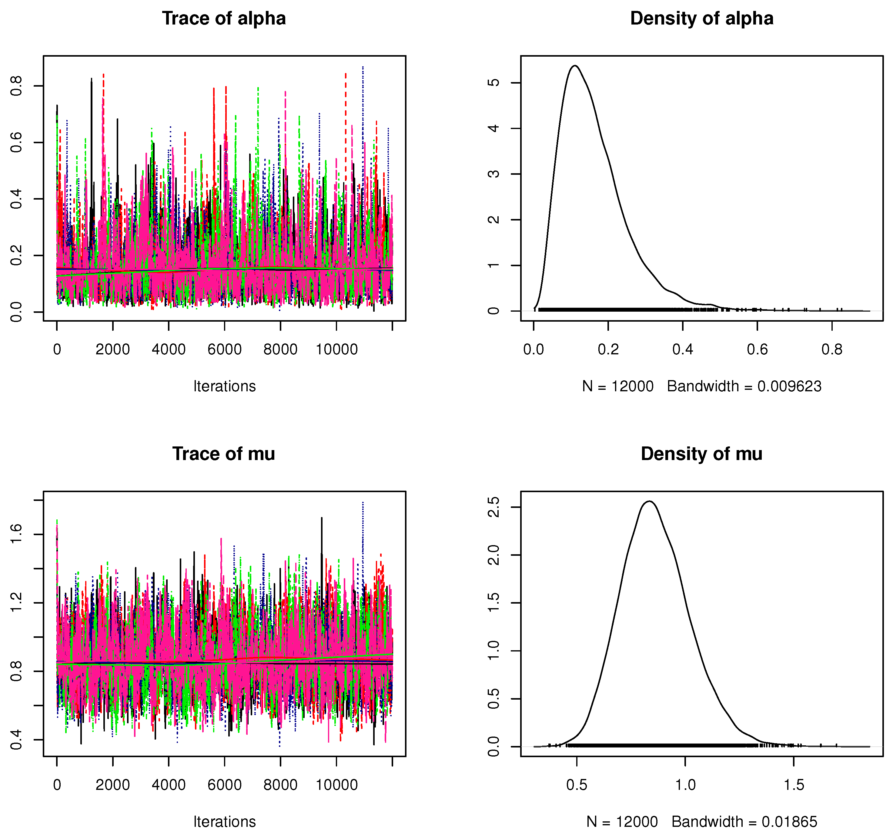
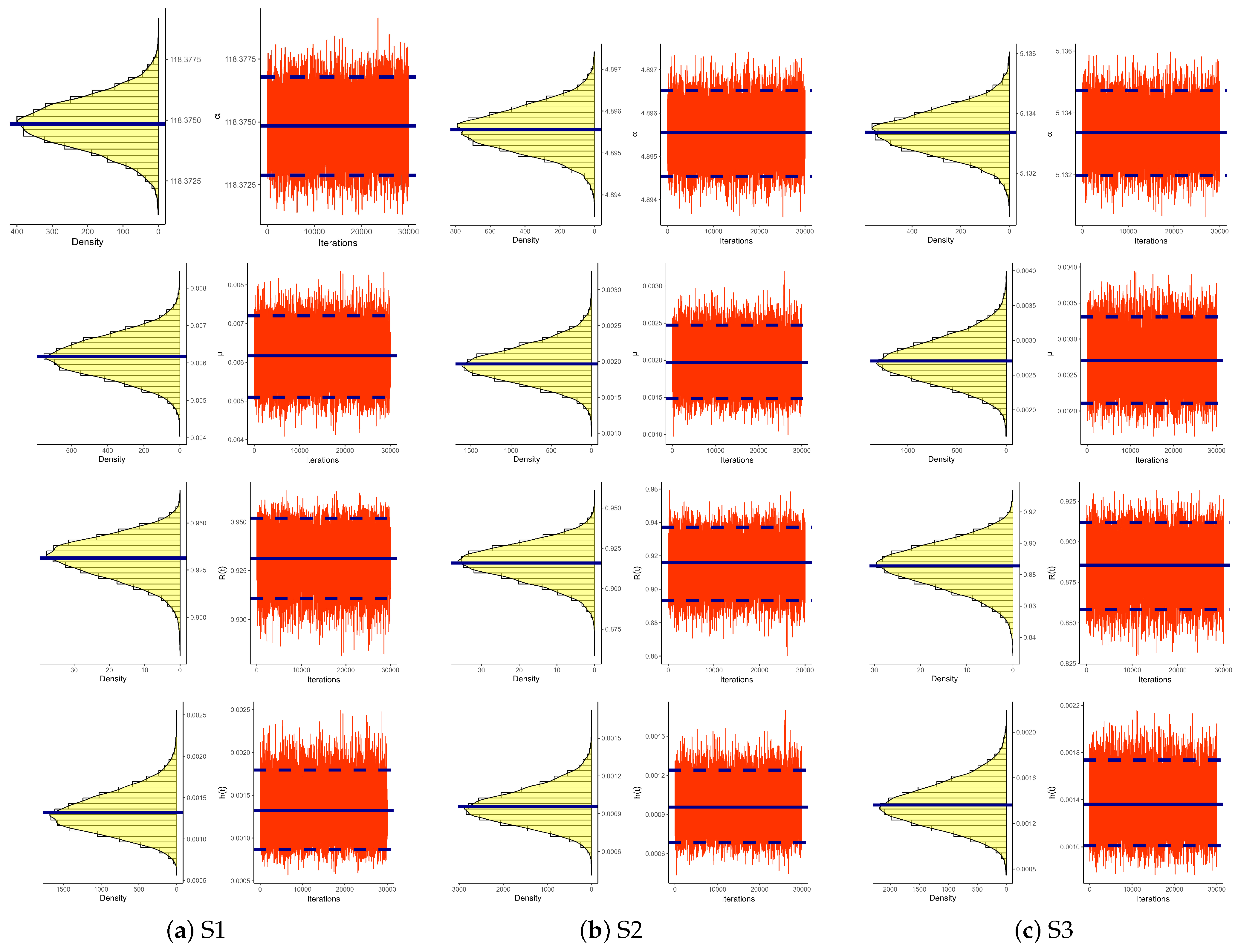
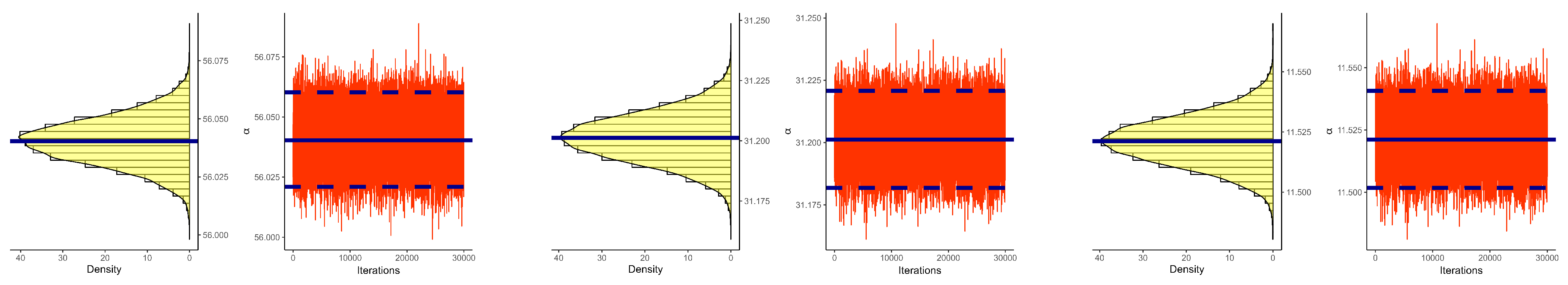
In Bayes MCMC computations, the convergence evaluation entails ensuring that the pattern, or chain, is the major concern in order to obtain a representative sample from the objective posterior distribution. For this objective, three convergence techniques are used: (i) the auto-correlation function (ACF), (ii) the Brooks–Gelman–Rubin (BGR) diagnostic, and (iii) the trace thinning-based (for example, we took the 5th point). Taking $(\alpha ,\mu )=(0.2,0.8)$, $(T_1,T_2)=(0.5,1.5)$, n[FP%] = 100[40%], $\underline{\mathrm{S}}=\left(1^{50}\right)$, and $(a_1,a_2,b_1,b_2)=(2,8,10,10)$, Figure 1 and Figure 2 show the suggested convergence (i)–(iii) operators. Figure 1a demonstrates that the lag autocorrelation inside every chain for every parameter stands for a high mixture of the generated chains and notable convergence for the posterior distribution. Figure 1b illustrates that there is a little variation in the variance within and variance between the resulting Markov chains. It additionally suggests that raising the quantity of the burn-in data is a successful strategy for reducing the impact of the starting values. Figure 2 signifies that the developed Markov chains of $\alpha$, $\mu$, $R\left(t\right)$, or $h\left(t\right)$ are suitably composite. As an outcome, the furnished point and interval estimations of $\alpha$, $\mu$, $R\left(t\right)$, and $h\left(t\right)$ are dependable and acceptable.

Specifically, for the parameter $\alpha$, the average estimate (Av.E) is expressed as:

$$Av.E\left(\alpha \right)=\frac{1}{1000}{\sum }_{i=1}^{1000}{\breve{\alpha }}^{\left(i\right)},$$

where ${\breve{\alpha }}^{\left(i\right)}$ is the estimate obtained from the ith sample. The root mean squared errors (RMSEs) and mean absolute biases (MABs) for comparing the various point estimates of $\alpha$ were obtained, respectively, as:

$$\mathrm{RMSE}\left(\breve{\alpha }\right)=\sqrt{\frac{1}{1000}{\sum }_{i=1}^{1000}{\left({\breve{\alpha }}^{\left(i\right)}-\alpha \right)}^2}$$

and

$$\mathrm{MAB}\left(\breve{\alpha }\right)=\frac{1}{1000}{\sum }_{i=1}^{1000}\left|{\breve{\alpha }}^{\left(i\right)}-\alpha \right|.$$

The assessment of interval estimates of $\alpha$ is based on their average confidence lengths (ACLs) and coverage percentages (CPs), which are defined, respectively, as:

$${\mathrm{ACL}}_{(1-\gamma )\%}\left(\alpha \right)=\frac{1}{1000}{\sum }_{i=1}^{1000}\left({\mathcal{U}}_{{\breve{\alpha }}^{\left(i\right)}}-{\mathcal{L}}_{{\breve{\alpha }}^{\left(i\right)}}\right)$$

and

$${\mathrm{CP}}_{(1-\gamma )\%}\left(\alpha \right)=\frac{1}{1000}{\sum }_{i=1}^{1000}{\mathit{I}}_{\left({\mathcal{L}}_{{\breve{\alpha }}^{\left(i\right)}};{\mathcal{U}}_{{\check{\alpha }}^{\left(i\right)}}\right)}^{\circ }\left(\alpha \right),$$

where ${\mathit{I}}^{\circ }(·)$ indicates the indicator operator and $\left(\mathcal{L}\right(·),\mathcal{U}(·\left)\right)$ represent the (lower, upper) boundaries of the $(1-\gamma )\%$ asymptotic (or credible) interval of $\alpha$. The Av.E, RMSE, MAB, ACL, and CP values for the other parameters can be easily calculated in the same way.

4.2. Simulation Results

A heatmap is a usual approach to displaying information. Colors are used to indicate individual values in a matrix in this tool. Therefore, Figure 3, Figure 4, Figure 5 and Figure 6 depict the acquired RMSEs, MABs, ACLs, and CPs of the various quantities using the $\mathsf{R}$ 4.2.2 programming language. Further descriptions of the methods on hand have been outlined on the ’$\mathsf{x}\text{-}\mathsf{axis}$’ line in Figure 3, Figure 4, Figure 5 and Figure 6 for concentration, including (for Prior 1 (say P1) as an example) the Bayesian MCMC estimates termed ”MCMC-P1” and the HPD interval estimates mentioned as ”HPD-P1”. In the Supplementary File, the corresponding numerical outcomes of $\alpha$, $\mu$, $R\left(t\right)$, and $h\left(t\right)$ are reported.

Figure 3, Figure 4, Figure 5 and Figure 6 show the following findings in regard to the lowest RMSE, MAB, and 95% ACL values, in addition to highest 95% CP values:

• The most important part is that the offered estimates of $\alpha$, $\mu$, $R\left(t\right)$, or $h\left(t\right)$ function adequately.
• As n (or FP%) increases, all estimates of $\alpha$, $\mu$, $R\left(t\right)$, and $h\left(t\right)$ behave satisfactorily. A similar comment is offered when ${\sum }_{i=1}^m{S}_i$ decreases. Therefore, to obtain a better result, we advise increasing the level of n (or FP%) as much as possible.
• As $T_i,i=1,2,$ increase, the RMSEs, MABs, and ACLs of various quantities decrease, while their CPs increase.
• Because of the gamma knowledge, the Bayesian estimates of various parameters outperform alternative estimates, as predicted. The same finding is drawn in the context of HPD intervals.
• Because Prior 2’s variance is less than Prior 1’s variance, MCMC simulations using Prior 2 yield greater precision estimates than others for $\alpha$, $\mu$, $R\left(t\right)$, or $h\left(t\right)$.
• When the proposed schemes A, B, and C are compared, it is discovered that the proposed estimates of $\alpha$ and $R\left(t\right)$ behave better with scheme A and those of $\mu$, and $h\left(t\right)$ behave better with scheme C than others.
• Therefore, to obtain high-quality estimates of any unknown life parameter in the presence of the proposed censored data, the experimenter must maximize the total test duration while taking into account the total cost of the test.
• To sum up, in the context of data acquired through improved adaptive progressive Type-II censoring, implementing a Bayesian framework via Metropolis–Hastings sampling is recommended for estimating the APE parameters or their reliability features.

5. Optimal Progressive Censoring

Up to this point, we have talked about statistical inferences of the unknown parameters of the APE distribution when the data are IAPT-IIC for a specific censoring strategy. The logical issue is how to select a specific censoring mechanism. Should we select a plan based just on ease of use or on statistical criteria?

Choosing an optimal censoring strategy in various scenarios has recently gained a lot of attention in the statistical literature. See, for instance, Wang and Yu [19] and Pradhan and Kundu [20]. It is essential for an investigator to find the ideal censoring strategy out of a number of alternative schemes, which is ideal in terms of how it supplies the greatest amount of information about the unknown parameters. The term “alternative schemes” relates to the numerous $(S_1,\dots ,S_m)$ choices for predetermined n, m, and threshold times. In this part, we present four criteria for identifying the best progressive censoring plan. For the vector $\mathbf{\Psi }$ with an asymptotic variance–covariance matrix denoted by ${\mathit{I}}^{-1}\left(\widehat{\mathbf{\Psi }}\right)$, the following criteria can be used to define optimality:

1.

Maximizing the trace of observed Fisher information matrix, denoted by $C_1$.

2.

Minimizing the trace of ${\mathit{I}}^{-1}\left(\widehat{\mathbf{\Psi }}\right)$ as

$$C_2=Min\left({\widehat{\sigma }}_{\alpha \alpha }^2+{\widehat{\sigma }}_{\mu \mu }^2\right).$$

3.

Minimizing the determinant of ${\mathit{I}}^{-1}\left(\widehat{\mathbf{\Psi }}\right)$ as

$$C_3=Min\left({\widehat{\sigma }}_{\alpha \alpha }^2{\widehat{\sigma }}_{\mu \mu }^2-{\widehat{\sigma }}_{\alpha \mu }^2\right).$$

4.

Minimizing the variance of the MLE of the logarithm of the qth quantile, with $0<q<1$, as

$$C_4=Min\left({\widehat{\sigma }}_{\alpha \alpha }^2{\widehat{Q}}_{\alpha }^2+2{\widehat{\sigma }}_{\alpha \mu }{\widehat{Q}}_{\alpha }{\widehat{Q}}_{\mu }+{\widehat{\sigma }}_{\mu \mu }^2{\widehat{Q}}_{\mu }^2\right),$$

where

$${\widehat{Q}}_{\alpha }=\frac{\widehat{\alpha }qlog\left(\widehat{\alpha }\right)-\widehat{\tau }log\left(\widehat{\tau }\right)}{\widehat{\tau }\widehat{\alpha }log\left(\widehat{\alpha }\right)\left[1-\frac{log\left(\widehat{\tau }\right)}{log\left(\widehat{\alpha }\right)}\right][log\left(\widehat{\tau }\right)-log\left(\widehat{\alpha }\right)]}$$

and

$${\widehat{Q}}_{\mu }=-\frac{1}{\widehat{\mu }},$$

with $\widehat{\tau }=1+q(\widehat{\alpha }-1)$.

6. Real-Life Applications

This section looks at three sets of real-world data from cancer, pathology, and mechanical fields of study to highlight the utility of the submitted estimation approaches and the relevance of the study’s aims to situations in reality.

6.1. Cancer Data Analysis

In this application, we look at a dataset that represents the survival periods of 121 people who were diagnosed with breast cancer from a large medical institution from 1929 to 1938. This dataset was provided by Lee [21] and recently reanalyzed by Alsolmi [22]. The Kolmogorov–Smirnov (KS) statistic (along with its P-value) is calculated to determine whether or not breast cancer data fit the APE distribution. Before going further, beyond multiplying each lifetime point of the given breast cancer data by 10 (for computational convenience and without loss of generality),

Table 1. Newly transformed breast cancer data.

3	3	40	50	56	62	63	66	68	74	75
84	84	103	110	118	122	123	135	144	144	148
155	157	162	163	165	168	172	173	175	179	198
204	209	210	210	211	230	234	236	240	240	279
282	291	300	310	310	320	350	350	370	370	370
380	380	380	390	390	400	400	400	410	410	410
420	430	430	430	440	450	450	460	460	470	480
490	510	510	510	520	540	550	560	570	580	590
600	600	600	610	620	650	650	670	670	680	690
780	800	830	880	890	900	930	960	1030	1050	1090
1090	1110	1150	1170	1250	1260	1270	1290	1290	1390	1540

lists a newly transformed breast cancer dataset.

As a consequence, from Table 1, the MLEs (with their standard errors (St.Ers) of $\alpha$ and $\mu$ are 7.6046 (3.8651) and 0.0033 (0.0003), respectively, with KS (P-value) 0.0528 (0.8885). That is, the APE model fits the breast cancer data rather satisfactorily. Employing the complete breast cancer data, Figure 7 depicts: (i) estimated/empirical reliability curves and (ii) the contour of the log-likelihood function. It supports the same KS facts and shows that the calculated MLEs $\widehat{\alpha }\cong 7.6046$ and $\widehat{\mu }\cong 0.0033$ might exist and are unique.

To examine the proposed estimation methodologies, from the complete breast cancer data, for fixed $m=41$ and various choices of $\underline{\mathrm{S}}$ and $T_i,i$ = 1, 2, different artificial IAPT-IIC samples of size $d_2$ are created; see

Table 2. Artificial IAPT-IIC samples from breast cancer data.

Sample	$\underline{\mathbf{S}}$	${\mathit{T}}_1\left({\mathit{d}}_1\right)$	${\mathit{T}}_2\left({\mathit{d}}_2\right)$	${\mathit{S}}^{*}$	T	Data
S1	$(4^{20},0^{21})$	185 (18)	250 (23)	26	250	3, 40, 56, 62, 68, 75, 84, 103, 118, 122, 135, 148, 155, 163, 165,
						168, 175, 179, 198, 211, 230, 236, 240
S2	$(0^{11},4^{20},0^{10})$	380 (27)	415 (31)	26	415	3, 3, 40, 50, 56, 62, 63, 66, 68, 74, 75, 84, 110, 118, 144, 148, 155,
						165, 168, 179, 198, 282, 291, 300, 310, 350, 370, 390, 390, 400, 410
S3	$(0^{21},4^{20})$	305 (30)	435 (40)	25	435	3, 3, 40, 50, 56, 62, 63, 66, 68, 74, 75, 84, 84, 103, 110, 118, 122,
						135, 148, 162, 165, 168, 175, 198, 210, 210, 211, 230, 279, 300,
						310, 350, 370, 370, 370, 380, 390, 410, 420, 430

. From Table 2, the MLEs and Bayesian MCMC estimates (along with their St.Ers), as well as the 95% ACI/HPD interval estimates (with their interval widths (IWs)) of $\alpha$, $\mu$, $R\left(t\right)$, and $h\left(t\right)$ (at $t=100$), are obtained and presented in

Table 3. Estimates of $\alpha$, $\mu$, $R\left(t\right)$, and $h\left(t\right)$ from breast cancer data.

Sample	Par.	MLE		MCMC		ACI			HPD
		Est.	St.Er	Est.	St.Er	Lower	Upper	IW	Lower	Upper	IW
S1	$\alpha$	118.37	4.2001	118.37	0.0010	110.14	126.61	16.464	118.37	118.38	0.0039
	$\mu$	0.0062	0.0006	0.0062	0.0005	0.0049	0.0075	0.0025	0.0051	0.0072	0.0021
	$R\left(100\right)$	0.9313	0.0127	0.9314	0.0107	0.9063	0.9563	0.0500	0.9106	0.9520	0.0413
	$h\left(100\right)$	0.0013	0.0003	0.0013	0.0002	0.0008	0.0019	0.0011	0.0009	0.0018	0.0009
S2	$\alpha$	4.8956	6.3436	4.8956	0.0005	0.0000	17.329	17.329	4.8945	4.8965	0.0020
	$\mu$	0.0020	0.0009	0.0020	0.0003	0.0001	0.0038	0.0037	0.0015	0.0025	0.0010
	$R\left(100\right)$	0.9152	0.0227	0.9158	0.0113	0.8708	0.9597	0.0889	0.8932	0.9371	0.0439
	$h\left(100\right)$	0.0010	0.0002	0.0010	0.0001	0.0006	0.0014	0.0008	0.0007	0.0012	0.0006
S3	$\alpha$	5.1334	3.4620	5.1334	0.0007	0.0000	11.919	11.919	5.1320	5.1347	0.0028
	$\mu$	0.0027	0.0006	0.0027	0.0003	0.0015	0.0040	0.0025	0.0021	0.0033	0.0012
	$R\left(100\right)$	0.8849	0.0217	0.8855	0.0137	0.8424	0.9274	0.0850	0.8584	0.9118	0.0534
	$h\left(100\right)$	0.0014	0.0002	0.0014	0.0002	0.0009	0.0018	0.0009	0.0010	0.0017	0.0007

. Because there is no prior information about $\alpha$ and $\mu$ in the supplied breast cancer dataset, the acquired Bayesian and HPD interval estimates are evaluated using improper gamma priors by running the MCMC sampler 40,000 times and skipping the initial 10,000 repetitions as burn-in. The unknown hyperparameters are set to 0.001 for computational aspect reasons. Table 3 reveals that the supplied MCMC estimates of $\alpha$, $\mu$, $R\left(t\right)$, or $h\left(t\right)$ act closely to the proposed frequentist estimates.

To show the existence and uniqueness of the offered MLEs of $\alpha$ and $\mu$, Figure 8 depicts the profile log-likelihood functions of $\alpha$ and $\mu$ for each simulated sample given in Table 2. It proves, based on all breast cancer samples, that the proposed MLEs of the two unknown parameters may exist and are unique.

Figure 9 depicts both the density and trace plots of the various parameters from each dataset presented in Table 2 to emphasize the convergence of MCMC runs. The solid line shows the Bayesian point estimate for discrimination, whereas the dotted line indicates the 95% HPD interval boundaries. The MCMC technique converges in a good way, as shown in Figure 9, and the recommended size of the burn-in sample is suitable to avoid the consequences of any suggested initial values. Furthermore, it demonstrates that the derived estimates of $\alpha$ and $\mu$ tend to be symmetrical, whereas those of $R\left(t\right)$ and $h\left(t\right)$ are negatively and positively skewed, respectively.

Further, to determine the best progressive censoring design among the proposed schemes used in samples Si for i = 1, 2, 3, the fitted optimum criteria $C_i,i$ = 1, 2, 3, 4 from the breast cancer data are provided in

Table 4. Optimum progressive censoring plans from breast cancer data.

Sample	${\mathit{C}}_1$	${\mathit{C}}_2$	${\mathit{C}}_3$	${\mathit{C}}_4$
$\mathit{q}\to$				0.3	0.6	0.9
S1	2,426,219.08342	17.64053	0.0000073	544.2602	1413.7016	4097.81283
S2	11,452,547.5681	40.24136	0.0000035	2535.639	25,723.104	244,288.613
S3	8,420,921.06268	11.98525	0.0000014	1086.728	5159.8135	35,074.1145

. It is evident that:

• Via criterion $C_1$; the middle censoring scheme $\underline{\mathrm{S}}=(0^{11},4^{20},0^{10})$ (in S2) is the optimum plan compared to others.
• Via criteria $C_i,i=2,3$; the right censoring scheme $\underline{\mathrm{S}}=(0^{21},4^{20})$ (in S3) is the optimum plan compared to others.
• Via criterion $C_4$ for all given values of q; the left censoring scheme $\underline{\mathrm{S}}=(4^{20},0^{21})$ (in S1) is the optimum plan compared to others.
• The ideal progressive censoring plans suggested based on the given breast cancer data confirm the same findings provided in Section 4.

6.2. Pathology Data Analysis

This application is concerned with analyzing a real-world dataset of 56 blood specimens from organ transplant patients. This dataset was originally offered by Hawkins [23] and was then studied by Nassar et al. [24]. The organ transplant blood (OTB) data are presented in

Table 5. Blood data from 56 organ transplant patients.

35	71	77	87	93	99	104	109	109	112	118	118
125	127	129	130	148	151	153	156	159	159	162	166
185	198	203	206	221	227	241	244	245	254	266	271
275	280	285	318	327	336	339	340	346	350	370	402
428	440	498	521	556	578	653	980

.

Before looking into the proposed estimators, one concern arises: namely, whether the OTB data match the APE lifetime model or not. Here, from Table 5, we have that the MLEs (with their St.Ers) of $\alpha$ and $\mu$ are 106.44 (118.88) and 0.0085 (0.0011), respectively, while the KS (P-value) is 0.0858 (0.8031). This result implies that the APE distribution fits the entire OTB reasonably well. To highlight the KS results and to show the existence and uniqueness of the offered MLEs $\widehat{\alpha }$ and $\widehat{\mu }$, based on the complete OTB data, Figure 10 confirms the calculated KS distance and shows that the estimates of 106.44 and 0.0085 for $\widehat{\alpha }$ and $\widehat{\mu }$ might exist and are unique.

Just as in our computation scenarios reported in Section 6.1, we report the outcomes of $\alpha$, $\mu$, $R\left(t\right)$, and $h\left(t\right)$ based on the real OTB dataset. Now, from the complete OTB data, we illustrate the various estimators of $\alpha$, $\mu$, $R\left(t\right)$, and $h\left(t\right)$. Taking $m=26$, using some choices of $T_i,i=1,2,$ and $\underline{\mathrm{S}}$, different IAPT-IIC samples are obtained; see

Table 6. Artificial IAPT-IIC samples from OTB data.

Sample	$\underline{\mathbf{S}}$	${\mathit{T}}_1\left({\mathit{d}}_1\right)$	${\mathit{T}}_2\left({\mathit{d}}_2\right)$	${\mathit{S}}^{*}$	T	Data
S1	$(3^{10},0^{16})$	128 (9)	200 (15)	14	200	35, 77, 99, 104, 109, 112, 118, 125, 127, 130, 151, 156, 159, 166, 185
S2	$(0^8,3^{10},0^8)$	225 (16)	260 (20)	12	260	35, 71, 77, 87, 93, 99, 104, 109, 109, 112, 127, 156, 185, 203, 206,
						221, 227, 244, 245, 254
S3	$(0^{16},3^{10})$	245 (23)	260 (25)	10	260	35, 71, 77, 87, 93, 99, 104, 109, 109, 112, 118, 118, 125, 127, 129,
						130, 148, 156, 159, 198, 221, 227, 244, 245, 254

. For each group in Table 5, the maximum likelihood and Bayesian estimates, St.Ers, two-sided 95% ACI/HPD interval estimates, and IWs of $\alpha$, $\mu$, $R\left(t\right)$, and $h\left(t\right)$ (at $t=50$) are obtained; see

Table 7. Estimates of $\alpha$, $\mu$, $R\left(t\right)$, and $h\left(t\right)$ from OTB data.

Sample	Par.	MLE		MCMC		ACI			HPD
		Est.	St.Er	Est.	St.Er	Lower	Upper	IW	Lower	Upper	IW
S1	$\alpha$	326.97	8.3911	326.97	0.0010	310.52	343.42	32.8923	326.97	326.97	0.0039
	$\mu$	0.0088	0.0010	0.0088	0.0007	0.0068	0.0109	0.0040	0.0074	0.0102	0.0028
	$R\left(50\right)$	0.9788	0.0046	0.9788	0.0033	0.9697	0.9878	0.0182	0.9724	0.9851	0.0127
	$h\left(50\right)$	0.0008	0.0002	0.0008	0.0001	0.0004	0.0012	0.0008	0.0005	0.0011	0.0006
S2	$\alpha$	154.79	5.9368	154.79	0.0010	143.15	166.42	23.272	154.79	154.79	0.0039
	$\mu$	0.0076	0.0008	0.0076	0.0006	0.0060	0.0092	0.0032	0.0063	0.0088	0.0025
	$R\left(50\right)$	0.9746	0.0046	0.9746	0.0035	0.9656	0.9836	0.0179	0.9678	0.9815	0.0137
	$h\left(50\right)$	0.0009	0.0002	0.0009	0.0001	0.0005	0.0012	0.0007	0.0006	0.0011	0.0006
S3	$\alpha$	157.27	5.9371	157.27	0.0010	145.63	168.91	23.273	157.27	157.27	0.0039
	$\mu$	0.0085	0.0008	0.0085	0.0006	0.0069	0.0102	0.0033	0.0072	0.0098	0.0025
	$R\left(50\right)$	0.9694	0.0051	0.9695	0.0039	0.9593	0.9795	0.0202	0.9620	0.9774	0.0153
	$h\left(50\right)$	0.0011	0.0002	0.0011	0.0002	0.0007	0.0015	0.0008	0.0007	0.0014	0.0006

. It suggests that all gained point (or credible) estimates of various parameters created using the likelihood and Bayesian approaches are relatively close to one other.

Figure 11 displays the log-likelihood functions of $\alpha$ and $\mu$, demonstrating that the MLEs may exist and are unique. Figure 12 shows trace plots for the last 30,000 MCMC simulated variants of $\alpha$, $\mu$, $R\left(t\right)$, and $h\left(t\right)$ for examining the process of convergence of the MCMC process. As a result, Figure 12 indicates that the suggested MCMC procedure converges satisfactorily for all unknown parameters. It also shows that the generated posterior estimates $\alpha$ and $\mu$, $R\left(t\right)$, or $h\left(t\right)$ are very symmetrical, while those are negatively and positively skewed, respectively.

Additionally, in

Table 8. Optimum PT-IIC plans from OTB data.

Sample	${\mathit{C}}_1$	${\mathit{C}}_2$	${\mathit{C}}_3$	${\mathit{C}}_4$
$\mathit{q}\to$				0.3	0.6	0.9
S1	953,893.91674	70.40987	0.000074	425.350	1012.303	2752.519
S2	1,461,398.3979	35.24607	0.000025	432.693	1094.945	3114.816
S3	1,420,349.7756	33.24870	0.000024	279.772	706.8901	2008.804

, the best progressive censoring design from OTB data is proposed based on the fitted optimum criteria $C_i,i=1,2,3,4$. It is evident that:

• Via criterion $C_1$; the middle censoring scheme $\underline{\mathrm{S}}=(0^8,3^{10},0^8)$ (in S2) is the optimum plan compared to others.
• Via criteria $C_i,i=2,3,4$; the right censoring scheme $\underline{\mathrm{S}}=(0^{16},3^{10})$ (in S3) is the optimum plan compared to others.
• The ideal progressive censoring plans suggested based on the given OTB data confirm the same findings as provided in Section 4.

6.3. Mechanical Data Analysis

In this application, we look at a real-world engineering data collection that contains 30 failures of repairable mechanical equipment (RME) components; see

Table 9. Failure times for 30 RME items.

0.11	0.30	0.40	0.45	0.59	0.63	0.70	0.71	0.74	0.77
0.94	1.06	1.17	1.23	1.23	1.24	1.43	1.46	1.49	1.74
1.82	1.86	1.97	2.23	2.37	2.46	2.63	3.46	4.36	4.73

. This dataset was originally provided by Murthy et al. [25] and reanalyzed by Elshahhat et al. [26].

First, in checking the fit status, the MLEs and the KS statistic (with its P-value) based on the RME items are obtained. The MLE (St.Er) of $\alpha$ is 21.369 (25.988) and of $\mu$ is 1.1725 (0.2292), while the KS (P-value) is 0.0784 (0.9927). This illustrates that the APE distribution is a suitable life model for the RME data. Figure 13 confirms the identical fit facts and proposes using the estimates $\widehat{\alpha }\cong 21.369$ and $\widehat{\mu }\cong 1.1725$ (which both might exist and are unique) as the basis for upcoming numerical calculations.

Similar to our computing scenarios mentioned in Section 6.1 and Section 6.2, we analyze all theoretical conclusions of $\alpha$, $\mu$, $R\left(t\right)$, and $h\left(t\right)$ based on the real RME dataset. To evaluate our acquired estimators, from the full RME dataset, we create different IAPT-IIC groups (when $m=15$) employing some values of $\underline{\mathrm{S}}$ and $T_i,i=1,2$; see

Table 10. Artificial IAPT-IIC samples from RME data.

Sample	$\underline{\mathbf{S}}$	${\mathit{T}}_1\left({\mathit{d}}_1\right)$	${\mathit{T}}_2\left({\mathit{d}}_2\right)$	${\mathit{S}}^{*}$	T	Data
S1	$(3^5,0^{10})$	0.65 (4)	1.45 (11)	7	1.45	0.11, 0.30, 0.45, 0.63, 0.71, 0.74, 0.77, 0.94, 1.06, 1.17, 1.43
S2	$(0^5,3^5,0^5)$	0.85 (8)	1.55 (13)	8	1.55	0.11, 0.30, 0.40, 0.45, 0.59, 0.63, 0.70, 0.77, 0.94, 1.17, 1.23, 1.43, 1.49
S3	$(0^{10},3^5)$	1.15 (12)	1.75 (15)	9	1.75	0.11, 0.30, 0.40, 0.45, 0.59, 0.63, 0.70, 0.71, 0.74, 0.77, 0.94, 1.06, 1.24, 1.49, 1.74

. All estimates are computed as presented in

Table 11. Estimates of $\alpha$, $\mu$, $R\left(t\right)$, and $h\left(t\right)$ from RME data.

Sample	Par.	MLE		MCMC		ACI			HPD
		Est.	St.Er	Est.	St.Er	Lower	Upper	IW	Lower	Upper	IW
S1	$\alpha$	56.041	17.245	56.040	0.0100	22.241	89.842	67.601	56.021	56.060	0.0393
	$\mu$	1.4314	0.2495	1.4304	0.0100	0.9425	1.9204	0.9779	1.4109	1.4497	0.0387
	$R\left(1\right)$	0.6291	0.0909	0.6295	0.0037	0.4510	0.8073	0.3563	0.6223	0.6368	0.0145
	$h\left(1\right)$	0.8516	0.2607	0.8505	0.0107	0.3405	1.3626	1.0221	0.8297	0.8711	0.0414
S2	$\alpha$	31.202	19.613	31.201	0.0100	0.0000	69.643	69.643	31.182	31.221	0.0390
	$\mu$	1.2064	0.2363	1.2052	0.0101	0.7433	1.6694	0.9261	1.1856	1.2249	0.0393
	$R\left(1\right)$	0.6642	0.0773	0.6646	0.0038	0.5126	0.8157	0.3031	0.6570	0.6720	0.0149
	$h\left(1\right)$	0.6900	0.2045	0.6889	0.0100	0.2892	1.0908	0.8016	0.6698	0.7086	0.0388
S3	$\alpha$	11.522	16.650	11.521	0.0100	0.0000	44.155	44.155	11.502	11.541	0.0390
	$\mu$	0.9460	0.3384	0.9448	0.0101	0.2828	1.6093	1.3265	0.9253	0.9646	0.0393
	$R\left(1\right)$	0.6711	0.0741	0.6716	0.0041	0.5259	0.8164	0.2905	0.6636	0.6794	0.0158
	$h\left(1\right)$	0.5671	0.1757	0.5660	0.0092	0.2227	0.9114	0.6886	0.5484	0.5842	0.0358

. The point estimates of $\alpha$, $\mu$, $R\left(t\right)$, and $h\left(t\right)$ appear to act closely due to the fact that they tend to be near each other. The overall trend of the interval estimates is identical. This is anticipated due to a lack of any extra previous information that could be helpful, leading to a little variation among the suggested frequentist and Bayesian estimations.

Figure 14 depicts the log-likelihood functions of $\alpha$ and $\mu$, demonstrating that the MLEs might exist and are unique. To evaluate the degree of convergence of the MCMC technique, the density and trace plots of various parameters are displayed in Figure 15. This indicates that the MCMC approach properly converges. It likewise demonstrates that the 30,000 modeled MCMC variant of various parameters are notably symmetrical.

The task of selecting the optimal progressive censoring plan on the basis of the RME data is also highlighted in

Table 12. Optimum progressive censoring plans from RME data.

Sample	${\mathit{C}}_1$	${\mathit{C}}_2$	${\mathit{C}}_3$	${\mathit{C}}_4$
$\mathit{q}\to$				0.3	0.6	0.9
S1	16.9820	297.46858	17.5167	0.02175	0.06127	0.19105
S2	24.4889	384.73270	15.7105	0.02451	0.07450	0.26544
S3	34.4151	277.32385	8.05819	0.03532	0.11442	0.72380

. It provides the following:

• Via criteria $C_i,i=1,2,3$; the right censoring scheme $\underline{\mathrm{S}}=(0^{10},3^5)$ (in S3) is the optimum plan compared to others.
• Via criterion $C_4$; the left censoring scheme $\underline{\mathrm{S}}=(3^5,0^{10})$ (in S1) is the optimum plan compared to others.
• The ideal progressive censoring plans proposed based on the given RME data confirm the same findings as reported in Section 4.

Finally, based on the analysis of the three mentioned real datasets, one can conclude that the right progressive censoring plan is the optimal progressive plan when compared with the left or middle ones. This is due to the fact that the right censoring plan has the longest lifetime, which means more observed values when compared with the other schemes. Moreover, we can draw the conclusion that the suggested inferential procedures perform well when applied to real-world data and provide an adequate interpretation of the alpha power exponential lifetime model when a sample is generated from the recommended censoring strategy.

7. Conclusions

In this study, we looked at how to estimate the alpha power exponential parameters, including reliability and hazard rate functions, when the data are improved and adaptive progressively Type-II censored. It was found that maximum likelihood estimates are unable to be acquired in clear form. As a consequence, the requisite estimates are calculated numerically by applying the Newton–Raphson technique. The approximate confidence intervals for each of the parameters are also presented using the asymptotic properties of the derived estimates. After that, the Bayesian estimation method is implemented to find the point and highest posterior density credible intervals. The Bayesian estimates are formed using the squared error loss function and the assumption of independent gamma priors. It should be noted that the joint posterior distribution cannot be deduced explicitly. As a result, we use the strategy of generating random samples from that distribution using the Markov chain Monte Carlo procedure to obtain the requisite estimates. Because the various estimates cannot be conceptually compared, simulation research is carried out to assess the statistical performance under various experimental conditions. We also provided the optimal sampling plans based on several criteria. Three illustrations representing the survival duration of breast cancer patients, blood specimens from organ transplant patients, and failure times of repairable mechanical equipment components were explored to demonstrate how the recommended methodologies may be utilized in practical scenarios. We believe that the conclusions and methods given here will be beneficial for reliability practitioners and will be used in future filtering mechanisms. In future work, it may be of interest to compare the selection process of the censoring plans used in the current work for the alpha power exponential distribution based on the improved adaptive progressive Type-II censoring scheme with other censoring schemes, like progressive Type-II and adaptive progressive Type-II censoring schemes. One can also consider the out-of-distribution cases, where the test data distribution is different from the training data distribution in the presence of improved adaptive progressively Type-II censored data. In this regard, see the work of Wang et al. [27]. Additional future work may be to test the behavior of extreme distributions in the case of the improved adaptive progressive Type-II censoring scheme.

References

1. Ng, H.K.T.; Chan, P.S.; Balakrishnan, N. Optimal progressive censoring plans for the Weibull distribution. Technometrics 2004, 46, 470–481. [Google Scholar] [CrossRef]
2. Kundu, D. Bayesian inference and life testing plan for the Weibull distribution in presence of progressive censoring. Technometrics 2008, 50, 144–154. [Google Scholar] [CrossRef]
3. Cramer, E.; Schmiedt, A.B. Progressively Type-II censored competing risks data from Lomax distributions. Comput. Stat. Data Anal. 2011, 55, 1285–1303. [Google Scholar] [CrossRef]
4. Dey, S.; Elshahhat, A.; Nassar, M. Analysis of progressive type-II censored gamma distribution. Comput. Stat. 2023, 38, 481–508. [Google Scholar] [CrossRef]
5. Balakrishnan, N.; Cramer, E. The Art of Progressive Censoring; Springer: Berlin/Heidelberg, Germany, 2014. [Google Scholar]
6. Kundu, D.; Joarder, A. Analysis of Type-II progressively hybrid censored data. Comput. Stat. Data Anal. 2006, 50, 2509–2528. [Google Scholar] [CrossRef]
7. Ng, H.K.T.; Kundu, D.; Chan, P.S. Statistical analysis of exponential lifetimes under an adaptive Type-II progressive censoring scheme. Nav. Res. Logist. 2009, 56, 687–698. [Google Scholar] [CrossRef]
8. Panahi, H.; Moradi, N. Estimation of the inverted exponentiated Rayleigh distribution based on adaptive Type II progressive hybrid censored sample. J. Comput. Appl. Math. 2020, 364, 112345. [Google Scholar] [CrossRef]
9. Kohansal, A.; Shoaee, S. Bayesian and classical estimation of reliability in a multicomponent stress-strength model under adaptive hybrid progressive censored data. Stat. Pap. 2021, 62, 309–359. [Google Scholar] [CrossRef]
10. Xiong, Z.; Gui, W. Classical and Bayesian inference of an exponentiated half-logistic distribution under adaptive type II progressive censoring. Entropy 2021, 23, 1558. [Google Scholar] [CrossRef]
11. Du, Y.; Gui, W. Statistical inference of adaptive type II progressive hybrid censored data with dependent competing risks under bivariate exponential distribution. J. Appl. Stat. 2022, 49, 3120–3140. [Google Scholar] [CrossRef]
12. Yan, W.; Li, P.; Yu, Y. Statistical inference for the reliability of Burr-XII distribution under improved adaptive Type-II progressive censoring. Appl. Math. Model. 2021, 95, 38–52. [Google Scholar] [CrossRef]
13. Mahdavi, A.; Kundu, D. A new method for generating distributions with an application to exponential distribution. Commun. Stat. Theory Methods 2017, 46, 6543–6557. [Google Scholar] [CrossRef]
14. Nassar, M.; Afify, A.Z.; Shakhatreh, M. Estimation methods of alpha power exponential distribution with applications to engineering and medical data. Pak. J. Stat. Oper. Res. 2020, 16, 149–166. [Google Scholar] [CrossRef]
15. Salah, M.M. On progressive Type-II censored samples from alpha power exponential distribution. J. Math. 2020, 2020, 2584184. [Google Scholar] [CrossRef]
16. Alotaibi, R.; Elshahhat, A.; Rezk, H.; Nassar, M. Inferences for Alpha Power Exponential Distribution Using Adaptive Progressively Type-II Hybrid Censored Data with Applications. Symmetry 2022, 14, 651. [Google Scholar] [CrossRef]
17. Henningsen, A.; Toomet, O. maxLik: A package for maximum likelihood estimation in R. Comput. Stat. 2011, 26, 443–458. [Google Scholar] [CrossRef]
18. Plummer, M.; Best, N.; Cowles, K.; Vines, K. CODA: Convergence diagnosis and output analysis for MCMC. R News 2006, 6, 7–11. [Google Scholar]
19. Wang, B.X.; Yu, K. Optimum plan for step-stress model with progressive type-II censoring. Test 2009, 18, 115–135. [Google Scholar] [CrossRef]
20. Pradhan, B.; Kundu, D. On progressively censored generalized exponential distribution. Test 2009, 18, 497–515. [Google Scholar] [CrossRef]
21. Lee, E.T. Statistical Methods for Survival Data Analysis; John Wiley: New York, NY, USA, 1992. [Google Scholar]
22. Alsolmi, M.M. Investigating cancer patients characteristics using a newly generated family of distributions. Alex. Eng. J. 2023, 77, 319–340. [Google Scholar] [CrossRef]
23. Hawkins, D.M. Diagnostics for conformity of paired quantitative measurements. Stat. Med. 2002, 21, 1913–1935. [Google Scholar] [CrossRef] [PubMed]
24. Nassar, M.; Alotaibi, R.; Elshahhat, A. Complexity analysis of E-Bayesian estimation under type-II censoring with application to organ transplant blood data. Symmetry 2022, 14, 1308. [Google Scholar] [CrossRef]
25. Murthy, D.N.P.; Xie, M.; Jiang, R. Weibull Models; Wiley Series in Probability and Statistics; Wiley: Hoboken, NJ, USA, 2004. [Google Scholar]
26. Elshahhat, A.; Almetwally, E.M.; Dey, S.; Mohammed, H.S. Analysis of WE Parameters of Life Using Adaptive-Progressively Type-II Hybrid Censored Mechanical Equipment Data. Axioms 2023, 12, 690. [Google Scholar] [CrossRef]
27. Wang, J.; Lan, C.; Liu, C.; Ouyang, Y.; Qin, T.; Lu, W.; Chen, Y.; Zeng, W.; Yu, P.S. Generalizing to Unseen Domains: A Survey on Domain Generalization. IEEE Trans. Knowl. Data Eng. 2022, 35, 8052–8072. [Google Scholar] [CrossRef]
Figure 1. The ACF and BGR plots of α , μ , R ( t ) , and h ( t ) in a Monte Carlo simulation.
Symmetry 15 02137 g001
Figure 2. Trace (left) and density (right) of plots α and μ in a Monte Carlo simulation.
Symmetry 15 02137 g002
Figure 3. Heatmap plots for α .
Symmetry 15 02137 g003
Figure 4. Heatmap plots for μ .
Symmetry 15 02137 g004
Figure 5. Heatmap plots for R ( t ) .
Symmetry 15 02137 g005
Figure 6. Heatmap plots for h ( t ) .
Symmetry 15 02137 g006
Figure 7. Empirical/fitted RF plot (left) and contour plot (right) based on breast cancer data.
Symmetry 15 02137 g007
Figure 8. The log-likelihood functions of α and μ from breast cancer data.
Symmetry 15 02137 g008aSymmetry 15 02137 g008b
Figure 9. Density (left) and trace (right) plots of α , μ , R ( t ) , and h ( t ) from breast cancer data.
Symmetry 15 02137 g009
Figure 10. Empirical/fitted RF plot (left) and contour plot (right) based on OTB data.
Symmetry 15 02137 g010
Figure 11. The log-likelihood functions of α and μ from OTB data.
Symmetry 15 02137 g011
Figure 12. Density (left) and trace (right) plots of α , μ , R ( t ) , and h ( t ) from OTB data.
Symmetry 15 02137 g012
Figure 13. Empirical/fitted RF plot (left) and contour plot (right) based on RME data.
Symmetry 15 02137 g013
Figure 14. The log-likelihood functions of α and μ from RME data.
Symmetry 15 02137 g014
Figure 15. Density (left) and trace (right) plots of α , μ , R ( t ) , and h ( t ) from RME data.
Symmetry 15 02137 g015aSymmetry 15 02137 g015b