Author Contributions
Conceptualization, H.M.A., H.A.-M., J.-T.S. and S.K.K.; Methodology, H.M.A., H.A.-M., J.-T.S. and S.K.K.; Software, H.M.A., H.A.-M., J.-T.S. and S.K.K.; Validation, H.M.A., H.A.-M., J.-T.S. and S.K.K.; Formal analysis, H.M.A., H.A.-M., J.-T.S. and S.K.K.; Investigation, H.M.A.; Data curation, H.A.-M. and J.-T.S.; Writing—original draft, H.M.A., H.A.-M., J.-T.S. and S.K.K.; Writing—review & editing, H.M.A.; Visualization, H.M.A., H.A.-M., J.-T.S. and S.K.K. All authors have read and agreed to the published version of the manuscript.
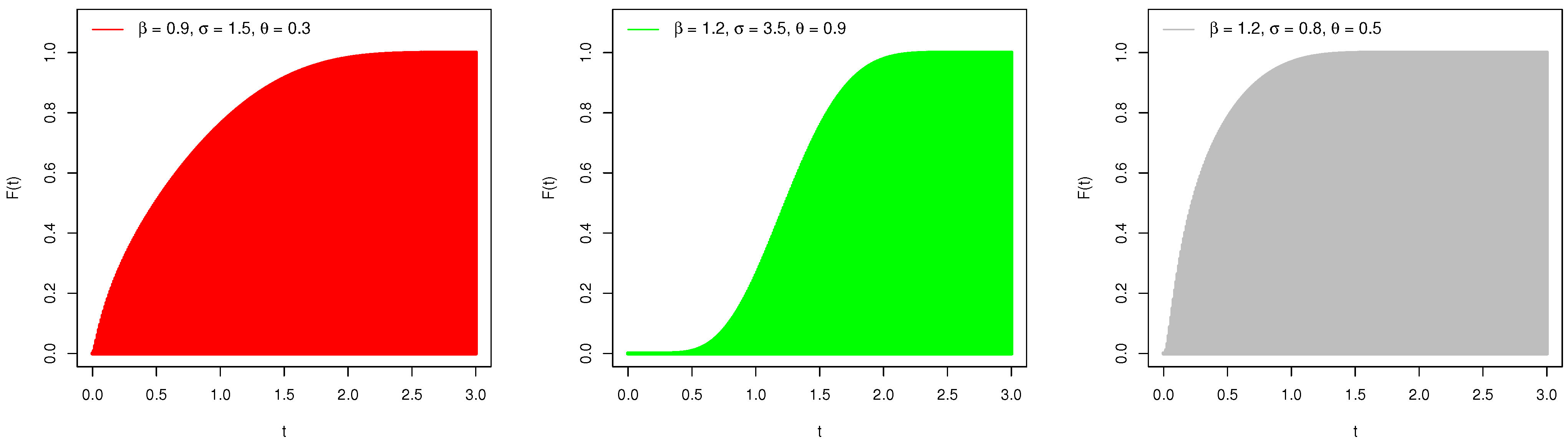
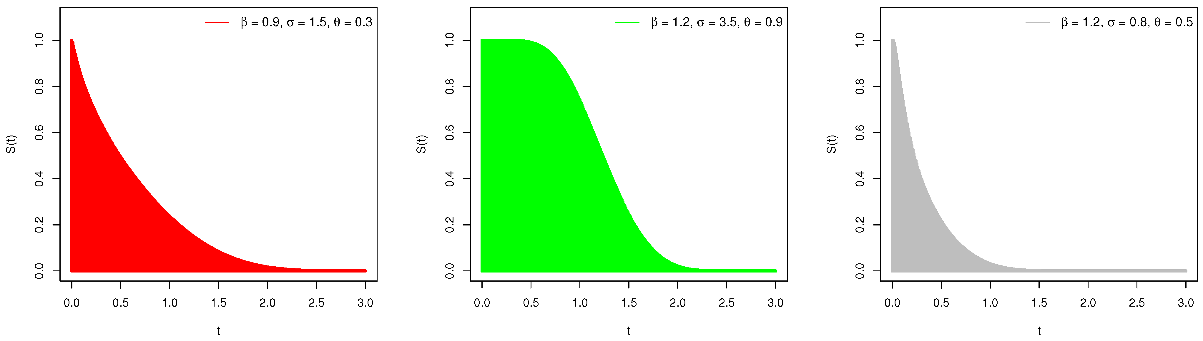
Figure 1.
The visual illustrations of and of the NTF-Weibull distribution for different values of , and .
Figure 1.
The visual illustrations of and of the NTF-Weibull distribution for different values of , and .
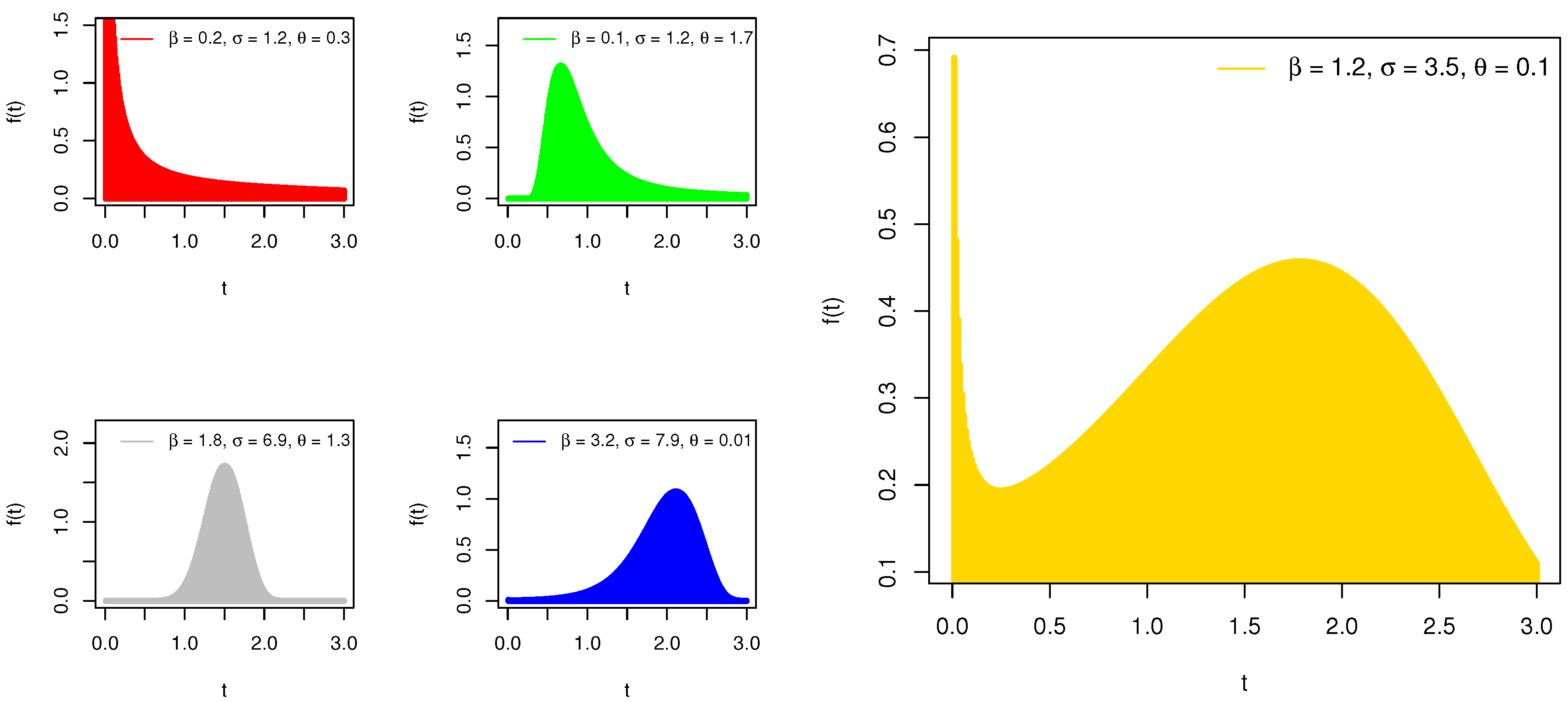
Figure 2.
The visual illustrations of of the NTF-Weibull distribution for different values of , and .
Figure 2.
The visual illustrations of of the NTF-Weibull distribution for different values of , and .
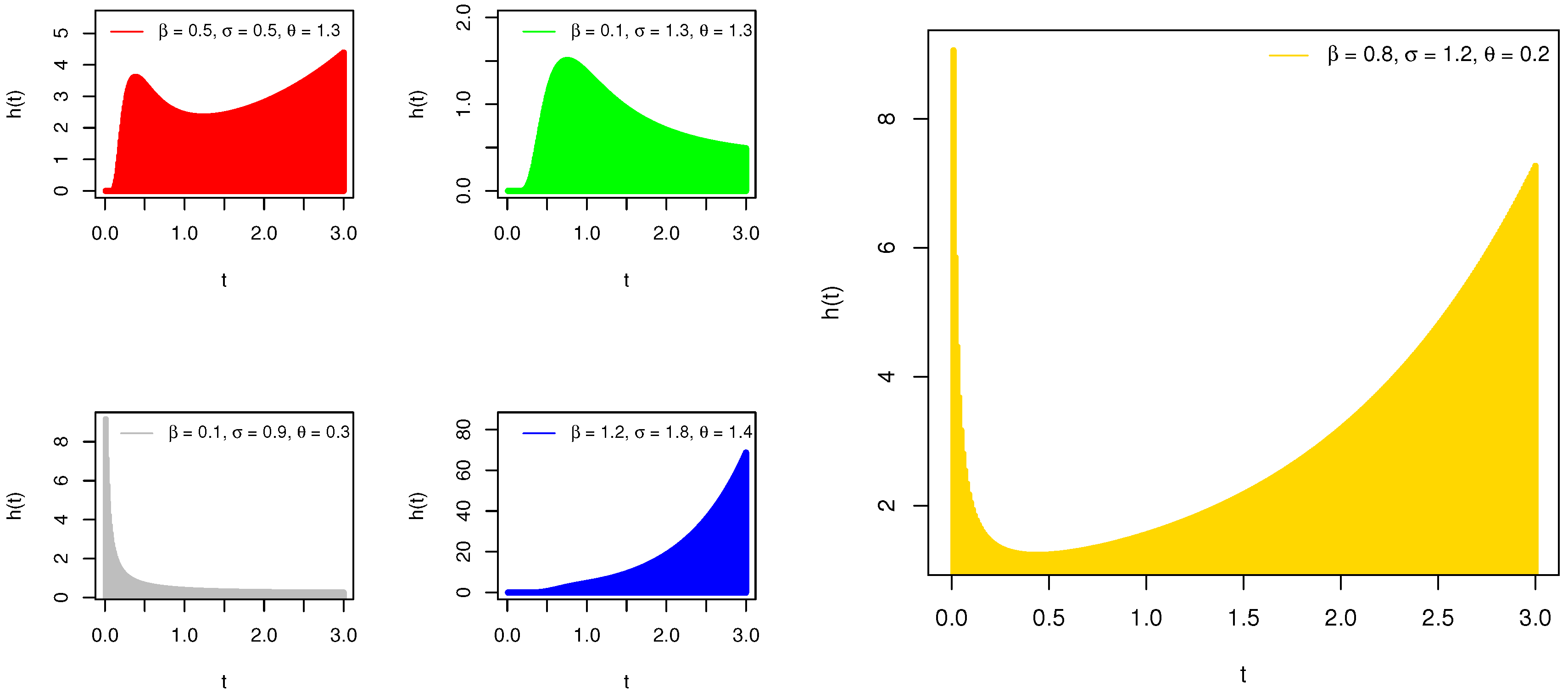
Figure 3.
The visual illustrations of of the NTF-Weibull distribution for different values of , and .
Figure 3.
The visual illustrations of of the NTF-Weibull distribution for different values of , and .
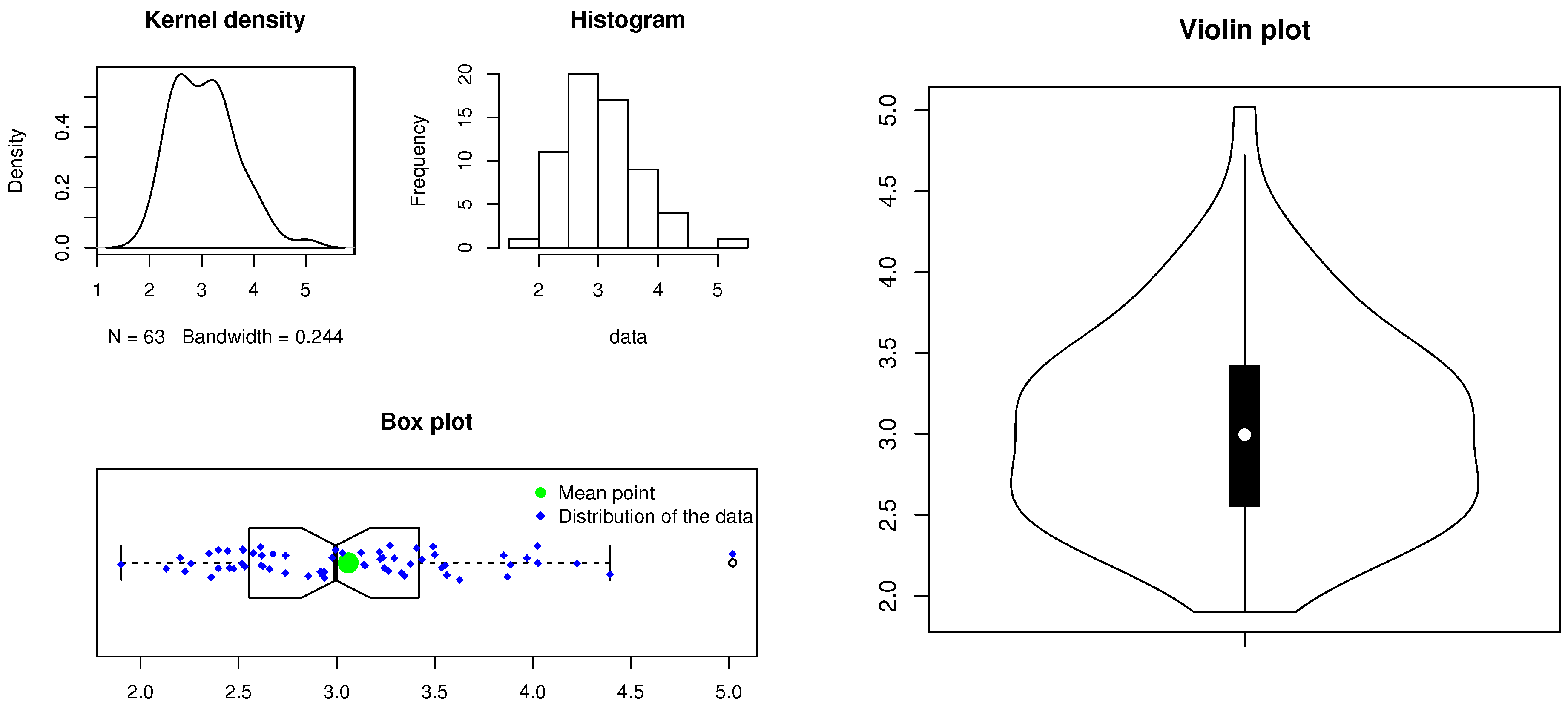
Figure 4.
Some descriptive plots of Data 1.
Figure 4.
Some descriptive plots of Data 1.
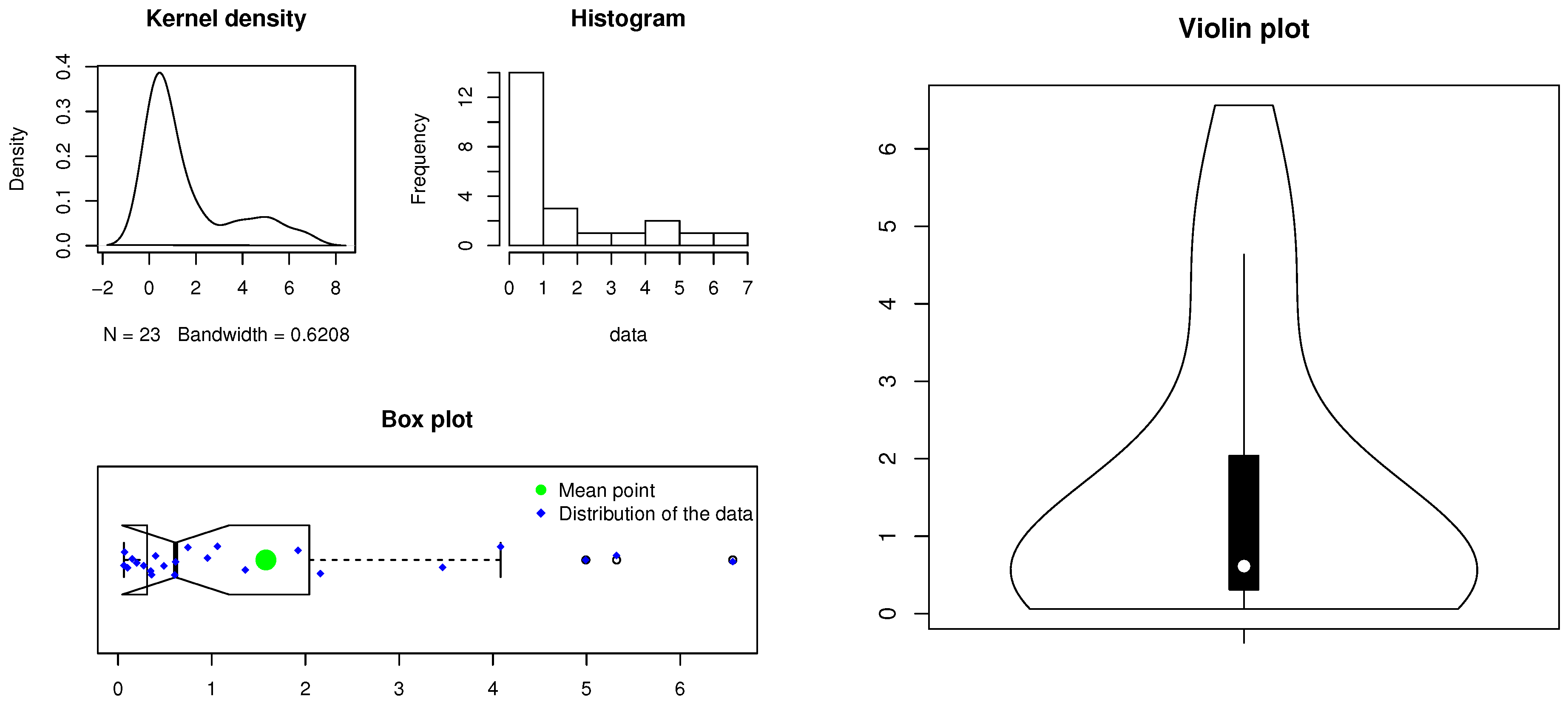
Figure 5.
Some descriptive plots of Data 2.
Figure 5.
Some descriptive plots of Data 2.
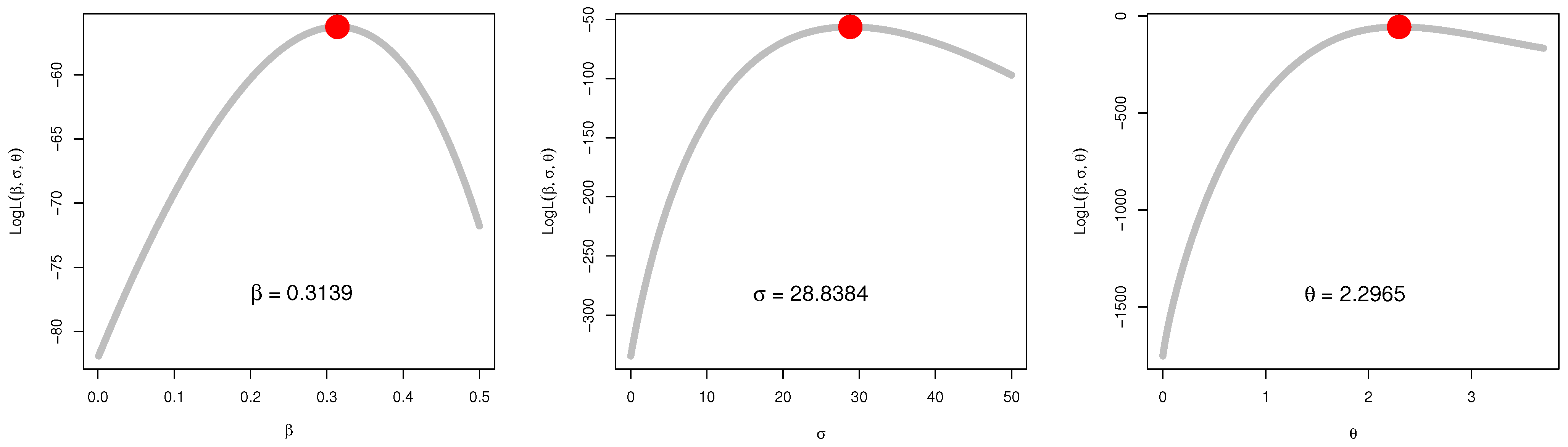
Figure 6.
The profiles of the LLF of and of the NTF-Weibull distribution for Data 1.
Figure 6.
The profiles of the LLF of and of the NTF-Weibull distribution for Data 1.
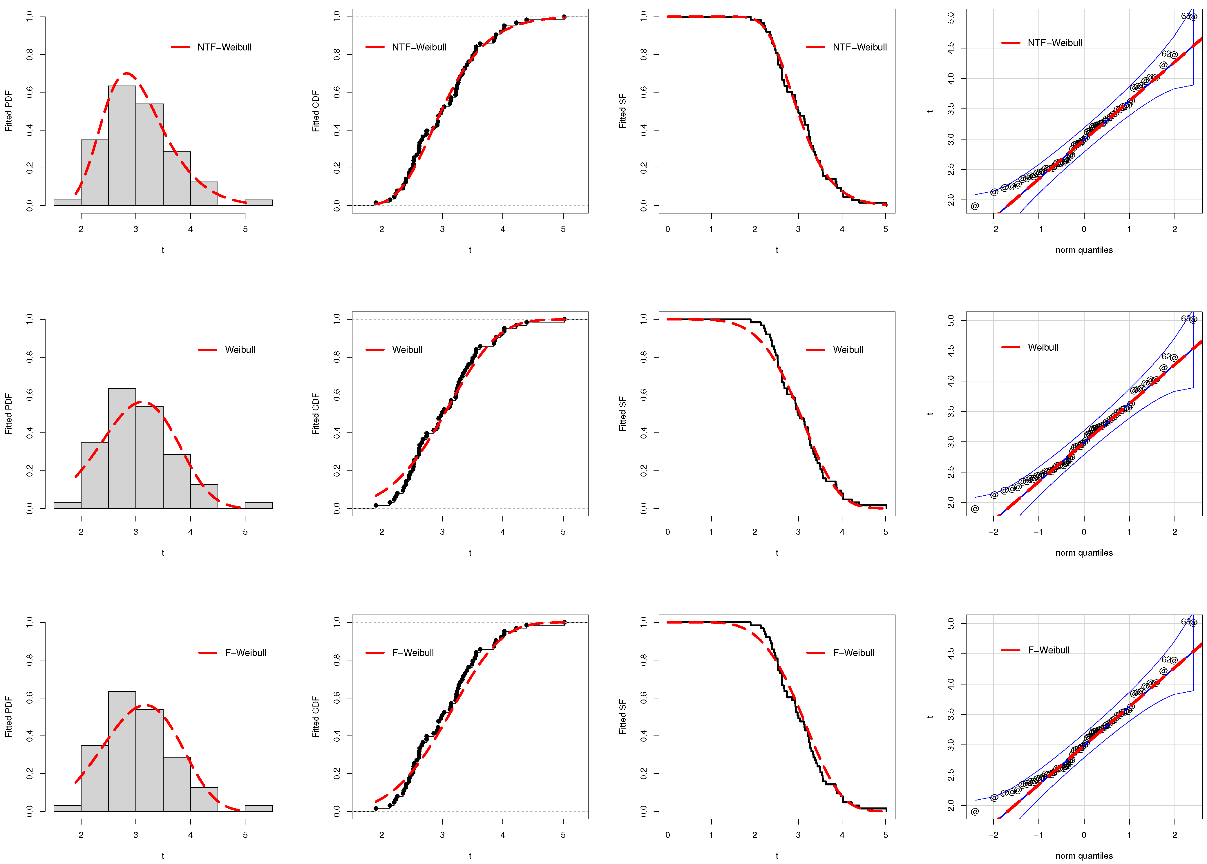
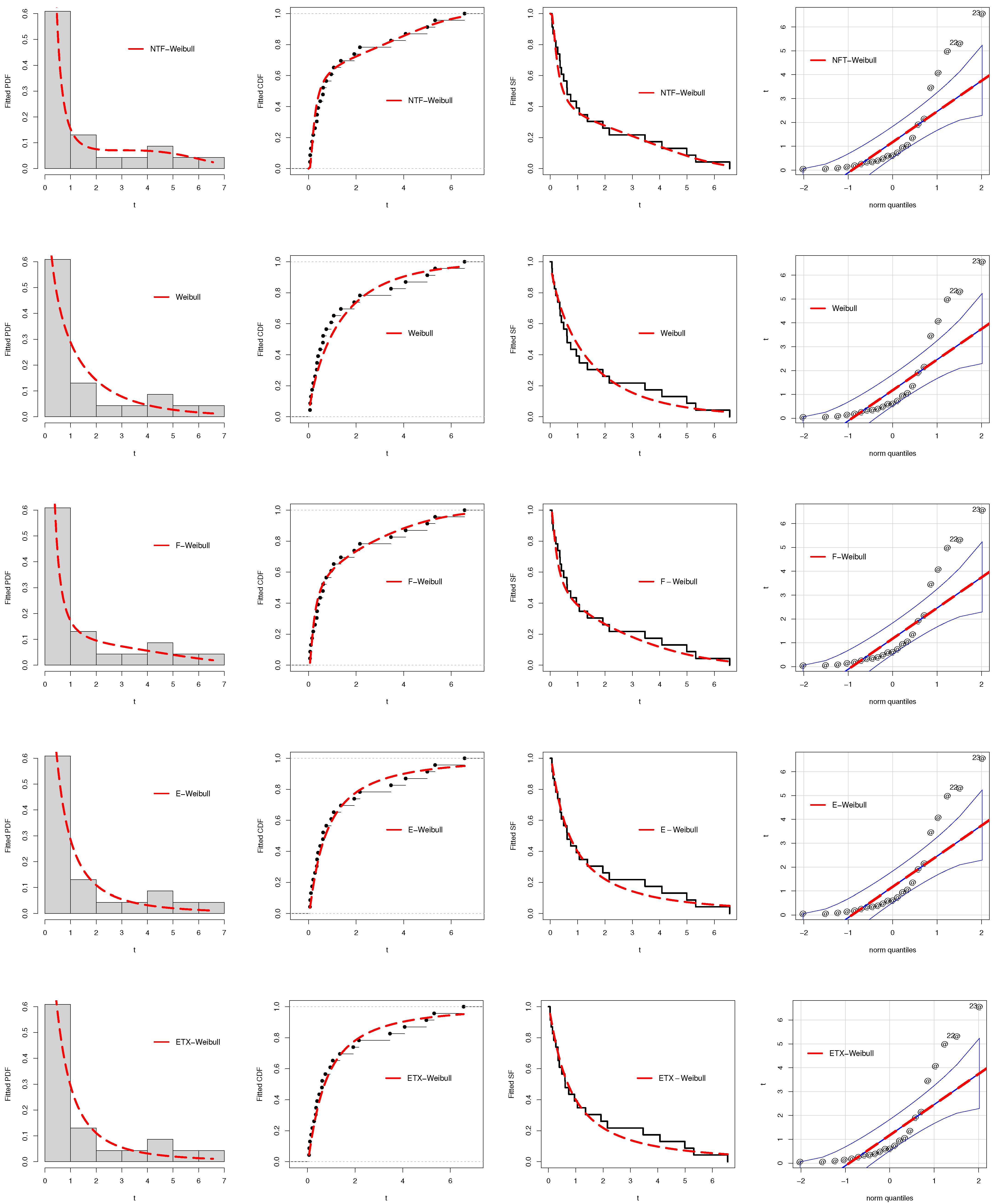
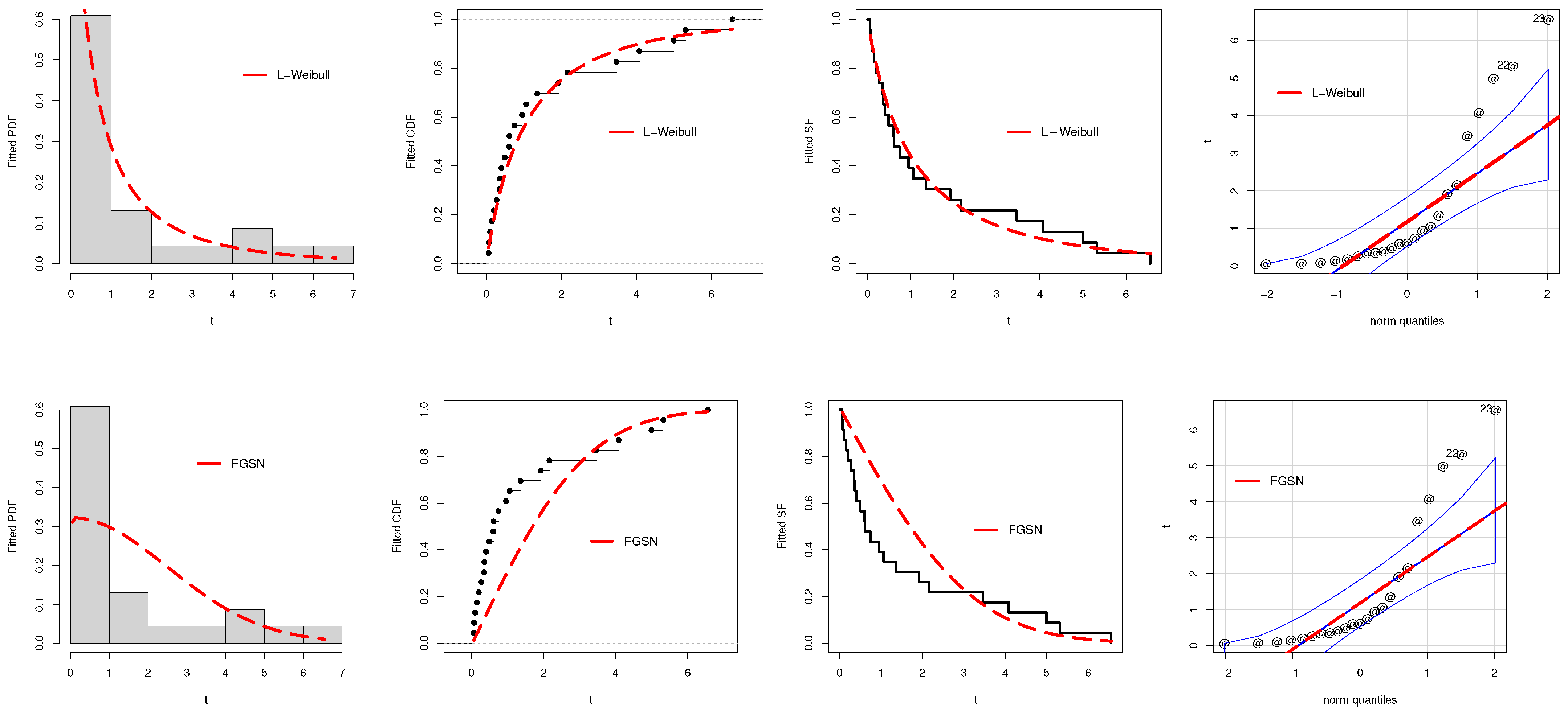
Figure 7.
The graphical evaluation of the fitted models using the mechanical engineering data set.
Figure 7.
The graphical evaluation of the fitted models using the mechanical engineering data set.
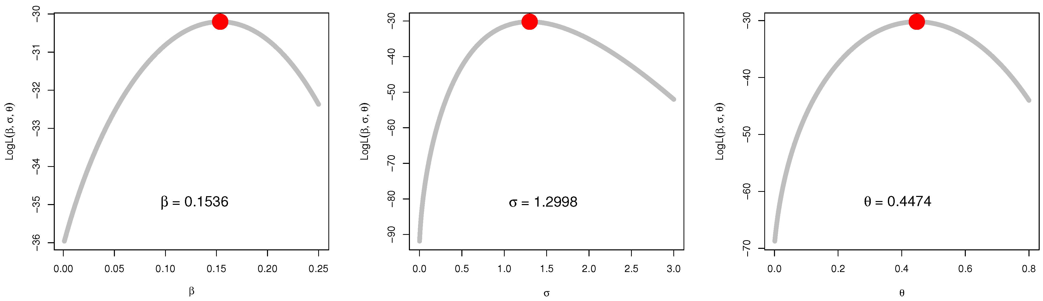
Figure 8.
The profiles of the LLF of and of the NTF-Weibull distribution using Data 2.
Figure 8.
The profiles of the LLF of and of the NTF-Weibull distribution using Data 2.
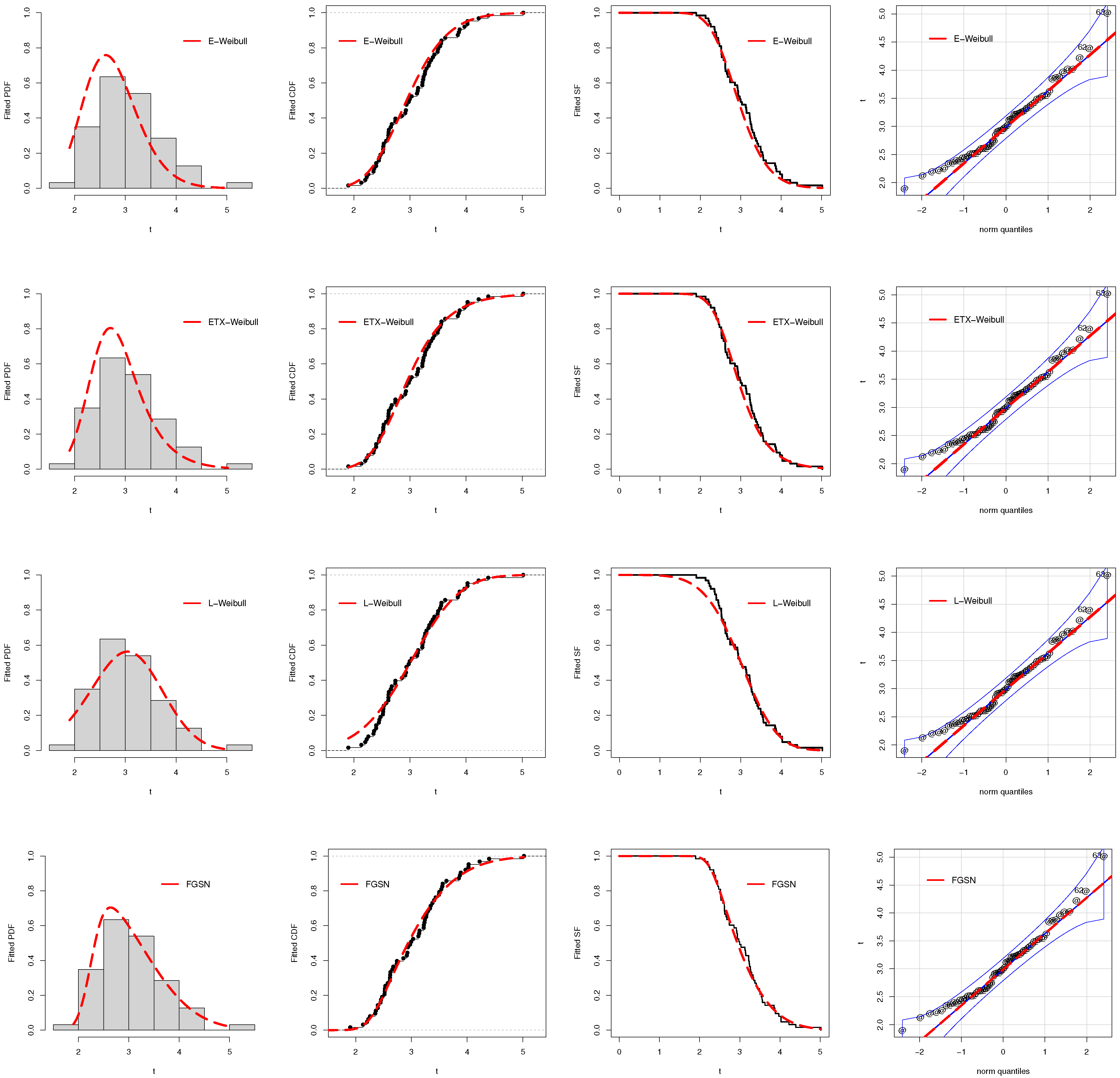
Figure 9.
The graphical evaluation of the fitted models using the reliability engineering data set.
Figure 9.
The graphical evaluation of the fitted models using the reliability engineering data set.
Table 1.
Simulation results for .
Table 1.
Simulation results for .
| n | Est. | Est. Par. | WLSE | OLSE | MLE | MPSE | CVME | ADE | RADE |
|---|
| 10 | | | | | | | | | |
| | | | | | | | | | |
| | | | | | | | | | |
| | MSE | | | | | | | | |
| | | | | | | | | | |
| | | | | | | | | | |
| | MRE | | | | | | | | |
| | | | | | | | | | |
| | | | | | | | | | |
| | | | | | | | | | |
| 20 | | | | | | | | | |
| | | | | | | | | | |
| | | | | | | | | | |
| | MSE | | | | | | | | |
| | | | | | | | | | |
| | | | | | | | | | |
| | MRE | | | | | | | | |
| | | | | | | | | | |
| | | | | | | | | | |
| | | | | | | | | | |
| | | | | | | | | | |
| 50 | | | | | | | | | |
| | | | | | | | | | |
| | | | | | | | | | |
| | MSE | | | | | | | | |
| | | | | | | | | | |
| | | | | | | | | | |
| | MRE | | | | | | | | |
| | | | | | | | | | |
| | | | | | | | | | |
| | | | | | | | | | |
| | | | | | | | | | |
| 80 | | | | | | | | | |
| | | | | | | | | | |
| | | | | | | | | | |
| | MSE | | | | | | | | |
| | | | | | | | | | |
| | | | | | | | | | |
| | MRE | | | | | | | | |
| | | | | | | | | | |
| | | | | | | | | | |
| | | | | | | | | | |
| | | | | | | | | | |
| 120 | | | | | | | | | |
| | | | | | | | | | |
| | | | | | | | | | |
| | MSE | | | | | | | | |
| | | | | | | | | | |
| | | | | | | | | | |
| | MRE | | | | | | | | |
| | | | | | | | | | |
| | | | | | | | | | |
| | | | | | | | | | |
| | | | | | | | | | |
| 200 | | | | | | | | | |
| | | | | | | | | | |
| | | | | | | | | | |
| | MSE | | | | | | | | |
| | | | | | | | | | |
| | | | | | | | | | |
| | MRE | | | | | | | | |
| | | | | | | | | | |
| | | | | | | | | | |
| | | | | | | | | | |
| | | | | | | | | | |
| 350 | | | | | | | | | |
| | | | | | | | | | |
| | | | | | | | | | |
| | MSE | | | | | | | | |
| | | | | | | | | | |
| | | | | | | | | | |
| | MRE | | | | | | | | |
| | | | | | | | | | |
| | | | | | | | | | |
| | | | | | | | | | |
Table 2.
Simulation results for .
Table 2.
Simulation results for .
| n | Est. | Est. Par. | WLSE | OLSE | MLE | MPSE | CVME | ADE | RADE |
|---|
| 10 | | | | | | | | | |
| | | | | | | | | | |
| | | | | | | | | | |
| | MSE | | | | | | | | |
| | | | | | | | | | |
| | | | | | | | | | |
| | MRE | | | | | | | | |
| | | | | | | | | | |
| | | | | | | | | | |
| | | | | | | | | | |
| 20 | | | | | | | | | |
| | | | | | | | | | |
| | | | | | | | | | |
| | MSE | | | | | | | | |
| | | | | | | | | | |
| | | | | | | | | | |
| | MRE | | | | | | | | |
| | | | | | | | | | |
| | | | | | | | | | |
| | | | | | | | | | |
| 50 | | | | | | | | | |
| | | | | | | | | | |
| | | | | | | | | | |
| | MSE | | | | | | | | |
| | | | | | | | | | |
| | | | | | | | | | |
| | MRE | | | | | | | | |
| | | | | | | | | | |
| | | | | | | | | | |
| | | | | | | | | | |
| 80 | | | | | | | | | |
| | | | | | | | | | |
| | | | | | | | | | |
| | MSE | | | | | | | | |
| | | | | | | | | | |
| | | | | | | | | | |
| | MRE | | | | | | | | |
| | | | | | | | | | |
| | | | | | | | | | |
| | | | | | | | | | |
| | | | | | | | | | |
| 120 | | | | | | | | | |
| | | | | | | | | | |
| | | | | | | | | | |
| | MSE | | | | | | | | |
| | | | | | | | | | |
| | | | | | | | | | |
| | MRE | | | | | | | | |
| | | | | | | | | | |
| | | | | | | | | | |
| | | | | | | | | | |
| | | | | | | | | | |
| 200 | | | | | | | | | |
| | | | | | | | | | |
| | | | | | | | | | |
| | MSE | | | | | | | | |
| | | | | | | | | | |
| | | | | | | | | | |
| | MRE | | | | | | | | |
| | | | | | | | | | |
| | | | | | | | | | |
| | | | | | | | | | |
| | | | | | | | | | |
| 350 | | | | | | | | | |
| | | | | | | | | | |
| | | | | | | | | | |
| | MSE | | | | | | | | |
| | | | | | | | | | |
| | | | | | | | | | |
| | MRE | | | | | | | | |
| | | | | | | | | | |
| | | | | | | | | | |
| | | | | | | | | | |
Table 3.
Simulation results for .
Table 3.
Simulation results for .
| n | Est. | Est. Par. | WLSE | OLSE | MLE | MPSE | CVME | ADE | RADE |
|---|
| 10 | | | | | | | | | |
| | | | | | | | | | |
| | | | | | | | | | |
| | MSE | | | | | | | | |
| | | | | | | | | | |
| | | | | | | | | | |
| | MRE | | | | | | | | |
| | | | | | | | | | |
| | | | | | | | | | |
| | | | | | | | | | |
| 20 | | | | | | | | | |
| | | | | | | | | | |
| | | | | | | | | | |
| | MSE | | | | | | | | |
| | | | | | | | | | |
| | | | | | | | | | |
| | MRE | | | | | | | | |
| | | | | | | | | | |
| | | | | | | | | | |
| | | | | | | | | | |
| 50 | | | | | | | | | |
| | | | | | | | | | |
| | | | | | | | | | |
| | MSE | | | | | | | | |
| | | | | | | | | | |
| | | | | | | | | | |
| | MRE | | | | | | | | |
| | | | | | | | | | |
| | | | | | | | | | |
| | | | | | | | | | |
| 80 | | | | | | | | | |
| | | | | | | | | | |
| | | | | | | | | | |
| | MSE | | | | | | | | |
| | | | | | | | | | |
| | | | | | | | | | |
| | MRE | | | | | | | | |
| | | | | | | | | | |
| | | | | | | | | | |
| | | | | | | | | | |
| 120 | | | | | | | | | |
| | | | | | | | | | |
| | | | | | | | | | |
| | MSE | | | | | | | | |
| | | | | | | | | | |
| | | | | | | | | | |
| | MRE | | | | | | | | |
| | | | | | | | | | |
| | | | | | | | | | |
| | | | | | | | | | |
| | | | | | | | | | |
| 200 | | | | | | | | | |
| | | | | | | | | | |
| | | | | | | | | | |
| | MSE | | | | | | | | |
| | | | | | | | | | |
| | | | | | | | | | |
| | MRE | | | | | | | | |
| | | | | | | | | | |
| | | | | | | | | | |
| | | | | | | | | | |
| | | | | | | | | | |
| 350 | | | | | | | | | |
| | | | | | | | | | |
| | | | | | | | | | |
| | MSE | | | | | | | | |
| | | | | | | | | | |
| | | | | | | | | | |
| | MRE | | | | | | | | |
| | | | | | | | | | |
| | | | | | | | | | |
| | | | | | | | | | |
Table 4.
Simulation results for .
Table 4.
Simulation results for .
| n | Est. | Est. Par. | WLSE | OLSE | MLE | MPSE | CVME | ADE | RADE |
|---|
| 10 | | | | | | | | | |
| | | | | | | | | | |
| | | | | | | | | | |
| | MSE | | | | | | | | |
| | | | | | | | | | |
| | | | | | | | | | |
| | MRE | | | | | | | | |
| | | | | | | | | | |
| | | | | | | | | | |
| | | | | | | | | | |
| 20 | | | | | | | | | |
| | | | | | | | | | |
| | | | | | | | | | |
| | MSE | | | | | | | | |
| | | | | | | | | | |
| | | | | | | | | | |
| | MRE | | | | | | | | |
| | | | | | | | | | |
| | | | | | | | | | |
| | | | | | | | | | |
| | | | | | | | | | |
| 50 | | | | | | | | | |
| | | | | | | | | | |
| | | | | | | | | | |
| | MSE | | | | | | | | |
| | | | | | | | | | |
| | | | | | | | | | |
| | MRE | | | | | | | | |
| | | | | | | | | | |
| | | | | | | | | | |
| | | | | | | | | | |
| | | | | | | | | | |
| 80 | | | | | | | | | |
| | | | | | | | | | |
| | | | | | | | | | |
| | MSE | | | | | | | | |
| | | | | | | | | | |
| | | | | | | | | | |
| | MRE | | | | | | | | |
| | | | | | | | | | |
| | | | | | | | | | |
| | | | | | | | | | |
| | | | | | | | | | |
| 120 | | | | | | | | | |
| | | | | | | | | | |
| | | | | | | | | | |
| | MSE | | | | | | | | |
| | | | | | | | | | |
| | | | | | | | | | |
| | MRE | | | | | | | | |
| | | | | | | | | | |
| | | | | | | | | | |
| | | | | | | | | | |
| | | | | | | | | | |
| 200 | | | | | | | | | |
| | | | | | | | | | |
| | | | | | | | | | |
| | MSE | | | | | | | | |
| | | | | | | | | | |
| | | | | | | | | | |
| | MRE | | | | | | | | |
| | | | | | | | | | |
| | | | | | | | | | |
| | | | | | | | | | |
| | | | | | | | | | |
| 350 | | | | | | | | | |
| | | | | | | | | | |
| | | | | | | | | | |
| | MSE | | | | | | | | |
| | | | | | | | | | |
| | | | | | | | | | |
| | MRE | | | | | | | | |
| | | | | | | | | | |
| | | | | | | | | | |
| | | | | | | | | | |
Table 5.
Simulation results for .
Table 5.
Simulation results for .
| n | Est. | Est. Par. | WLSE | OLSE | MLE | MPSE | CVME | ADE | RADE |
|---|
| 10 | | | | | | | | | |
| | | | | | | | | | |
| | | | | | | | | | |
| | MSE | | | | | | | | |
| | | | | | | | | | |
| | | | | | | | | | |
| | MRE | | | | | | | | |
| | | | | | | | | | |
| | | | | | | | | | |
| | | | | | | | | | |
| 20 | | | | | | | | | |
| | | | | | | | | | |
| | | | | | | | | | |
| | MSE | | | | | | | | |
| | | | | | | | | | |
| | | | | | | | | | |
| | MRE | | | | | | | | |
| | | | | | | | | | |
| | | | | | | | | | |
| | | | | | | | | | |
| 50 | | | | | | | | | |
| | | | | | | | | | |
| | | | | | | | | | |
| | MSE | | | | | | | | |
| | | | | | | | | | |
| | | | | | | | | | |
| | MRE | | | | | | | | |
| | | | | | | | | | |
| | | | | | | | | | |
| | | | | | | | | | |
| | | | | | | | | | |
| 80 | | | | | | | | | |
| | | | | | | | | | |
| | | | | | | | | | |
| | MSE | | | | | | | | |
| | | | | | | | | | |
| | | | | | | | | | |
| | MRE | | | | | | | | |
| | | | | | | | | | |
| | | | | | | | | | |
| | | | | | | | | | |
| | | | | | | | | | |
| 120 | | | | | | | | | |
| | | | | | | | | | |
| | | | | | | | | | |
| | MSE | | | | | | | | |
| | | | | | | | | | |
| | | | | | | | | | |
| | MRE | | | | | | | | |
| | | | | | | | | | |
| | | | | | | | | | |
| | | | | | | | | | |
| | | | | | | | | | |
| 200 | | | | | | | | | |
| | | | | | | | | | |
| | | | | | | | | | |
| | MSE | | | | | | | | |
| | | | | | | | | | |
| | | | | | | | | | |
| | MRE | | | | | | | | |
| | | | | | | | | | |
| | | | | | | | | | |
| | | | | | | | | | |
| | | | | | | | | | |
| 350 | | | | | | | | | |
| | | | | | | | | | |
| | | | | | | | | | |
| | MSE | | | | | | | | |
| | | | | | | | | | |
| | | | | | | | | | |
| | MRE | | | | | | | | |
| | | | | | | | | | |
| | | | | | | | | | |
| | | | | | | | | | |
Table 6.
Simulation results for .
Table 6.
Simulation results for .
| n | Est. | Est. Par. | WLSE | OLSE | MLE | MPSE | CVME | ADE | RADE |
|---|
| 10 | | | | | | | | | |
| | | | | | | | | | |
| | | | | | | | | | |
| | MSE | | | | | | | | |
| | | | | | | | | | |
| | | | | | | | | | |
| | MRE | | | | | | | | |
| | | | | | | | | | |
| | | | | | | | | | |
| | | | | | | | | | |
| 20 | | | | | | | | | |
| | | | | | | | | | |
| | | | | | | | | | |
| | MSE | | | | | | | | |
| | | | | | | | | | |
| | | | | | | | | | |
| | MRE | | | | | | | | |
| | | | | | | | | | |
| | | | | | | | | | |
| | | | | | | | | | |
| 50 | | | | | | | | | |
| | | | | | | | | | |
| | | | | | | | | | |
| | MSE | | | | | | | | |
| | | | | | | | | | |
| | | | | | | | | | |
| | MRE | | | | | | | | |
| | | | | | | | | | |
| | | | | | | | | | |
| | | | | | | | | | |
| 80 | | | | | | | | | |
| | | | | | | | | | |
| | | | | | | | | | |
| | MSE | | | | | | | | |
| | | | | | | | | | |
| | | | | | | | | | |
| | MRE | | | | | | | | |
| | | | | | | | | | |
| | | | | | | | | | |
| | | | | | | | | | |
| 120 | | | | | | | | | |
| | | | | | | | | | |
| | | | | | | | | | |
| | MSE | | | | | | | | |
| | | | | | | | | | |
| | | | | | | | | | |
| | MRE | | | | | | | | |
| | | | | | | | | | |
| | | | | | | | | | |
| | | | | | | | | | |
| | | | | | | | | | |
| 200 | | | | | | | | | |
| | | | | | | | | | |
| | | | | | | | | | |
| | MSE | | | | | | | | |
| | | | | | | | | | |
| | | | | | | | | | |
| | MRE | | | | | | | | |
| | | | | | | | | | |
| | | | | | | | | | |
| | | | | | | | | | |
| | | | | | | | | | |
| 350 | | | | | | | | | |
| | | | | | | | | | |
| | | | | | | | | | |
| | MSE | | | | | | | | |
| | | | | | | | | | |
| | | | | | | | | | |
| | MRE | | | | | | | | |
| | | | | | | | | | |
| | | | | | | | | | |
| | | | | | | | | | |
Table 7.
Partial and overall ranks of the classical estimation methods for several parametric values.
Table 7.
Partial and overall ranks of the classical estimation methods for several parametric values.
| n | WLSE | OLSE | MLE | MPSE | CVME | ADE | RADE |
|---|
| | 10 | 4 | 5 | 2.5 | 1 | 7 | 2.5 | 6 |
| | 20 | 4 | 6 | 2 | 1 | 7 | 3 | 5 |
| | 50 | 4 | 6 | 1 | 2 | 7 | 3 | 5 |
| 80 | 4 | 6 | 1 | 2 | 7 | 3 | 5 |
| | 120 | 4 | 5.5 | 1 | 2 | 7 | 3 | 5.5 |
| | 200 | 4 | 7 | 2 | 1 | 6 | 3 | 5 |
| | 350 | 3 | 5 | 1 | 2 | 7 | 4 | 6 |
| | 10 | 4 | 5 | 1 | 2 | 7 | 3 | 6 |
| | 20 | 5 | 6 | 1 | 2 | 7 | 3 | 4 |
| | 50 | 5 | 6 | 1 | 2 | 7 | 3 | 4 |
| 80 | 5 | 6 | 1 | 2 | 7 | 3 | 4 |
| | 120 | 4 | 6 | 1 | 2 | 7 | 3 | 5 |
| | 200 | 4.5 | 7 | 1 | 2 | 6 | 3 | 4.5 |
| | 350 | 4 | 6 | 2 | 1 | 7 | 3 | 5 |
| | 10 | 4 | 6 | 1 | 2 | 7 | 3 | 5 |
| | 20 | 5 | 6 | 2 | 1 | 7 | 3 | 4 |
| | 50 | 5 | 6 | 2 | 1 | 7 | 3 | 4 |
| 80 | 5 | 7 | 2 | 1 | 6 | 3 | 4 |
| | 120 | 5 | 6 | 2 | 1 | 7 | 3 | 4 |
| | 200 | 5 | 6 | 2 | 1 | 7 | 3 | 4 |
| | 350 | 4.5 | 6 | 2 | 1 | 7 | 3 | 4.5 |
| | 10 | 4 | 5 | 1 | 2 | 6.5 | 3 | 6.5 |
| | 20 | 4 | 6 | 1 | 2 | 7 | 3 | 5 |
| | 50 | 4 | 7 | 2 | 1 | 6 | 3 | 5 |
| 80 | 4 | 6 | 2 | 1 | 7 | 3 | 5 |
| | 120 | 4 | 5.5 | 2 | 1 | 7 | 3 | 5.5 |
| | 200 | 4 | 6 | 1 | 2 | 7 | 3 | 5 |
| | 350 | 4 | 7 | 1 | 2 | 6 | 3 | 5 |
| | 10 | 4 | 5 | 2 | 1 | 7 | 3 | 6 |
| | 20 | 5 | 6 | 1 | 2 | 7 | 3 | 4 |
| | 50 | 5 | 7 | 1 | 2 | 6 | 3 | 4 |
| 80 | 5 | 6 | 1 | 2 | 7 | 3 | 4 |
| | 120 | 4 | 7 | 2 | 1 | 6 | 3 | 5 |
| | 200 | 4 | 7 | 1 | 2 | 6 | 3 | 5 |
| | 350 | 4 | 6 | 2 | 1 | 7 | 3 | 5 |
| | 10 | 4 | 5.5 | 2.5 | 1 | 7 | 2.5 | 5.5 |
| | 20 | 5 | 6 | 1 | 2 | 7 | 3 | 4 |
| | 50 | 5 | 7 | 2 | 1 | 6 | 3 | 4 |
| 80 | 5 | 6 | 1 | 2 | 7 | 3 | 4 |
| | 120 | 5 | 6 | 2 | 1 | 7 | 3 | 4 |
| | 200 | 5 | 7 | 2 | 1 | 6 | 3 | 4 |
| | 350 | 5 | 6 | 2 | 1 | 7 | 3 | 4 |
| | 10 | 4 | 5 | 2 | 1 | 6 | 3 | 7 |
| | 20 | 4 | 6 | 1 | 2 | 7 | 3 | 5 |
| | 50 | 4 | 6 | 1 | 2 | 7 | 3 | 5 |
| 80 | 4 | 7 | 1 | 2 | 6 | 3 | 5 |
| | 120 | 4 | 5.5 | 1 | 2 | 7 | 3 | 5.5 |
| | 200 | 4 | 5.5 | 1 | 2 | 7 | 3 | 5.5 |
| | 350 | 4 | 7 | 1 | 2 | 6 | 3 | 5 |
| | 10 | 4 | 5 | 1 | 2 | 7 | 3 | 6 |
| | 20 | 4.5 | 6 | 1 | 2 | 7 | 3 | 4.5 |
| | 50 | 5 | 6 | 1 | 2 | 7 | 3 | 4 |
| 80 | 5 | 6 | 1 | 2 | 7 | 3 | 4 |
| | 120 | 5 | 6 | 1 | 2 | 7 | 3 | 4 |
| | 200 | 4 | 6 | 1 | 2 | 7 | 3 | 5 |
| | 350 | 4 | 7 | 2 | 1 | 6 | 3 | 5 |
| | 10 | 4 | 5 | 2 | 1 | 7 | 3 | 6 |
| | 20 | 5 | 6 | 1 | 2 | 7 | 3 | 4 |
| | 50 | 5 | 6 | 2 | 1 | 7 | 3 | 4 |
| 80 | 5 | 6 | 2 | 1 | 7 | 3 | 4 |
| | 120 | 5 | 7 | 2 | 1 | 6 | 3 | 4 |
| | 200 | 5 | 7 | 2 | 1 | 6 | 3.5 | 3.5 |
| | 350 | 5 | 6 | 2 | 1 | 7 | 4 | 3 |
| | 10 | 4 | 5 | 2 | 1 | 7 | 3 | 6 |
| | 20 | 4 | 6 | 1 | 2 | 7 | 3 | 5 |
| | 50 | 4 | 6 | 1 | 2 | 7 | 3 | 5 |
| 80 | 4 | 6 | 1 | 2 | 7 | 3 | 5 |
| | 120 | 4 | 5 | 1 | 2 | 6 | 3 | 7 |
| | 200 | 4 | 5.5 | 1 | 2 | 7 | 3 | 5.5 |
| | 350 | 4 | 5 | 1 | 2 | 6.5 | 3 | 6.5 |
| | 10 | 4 | 5.5 | 1 | 2 | 7 | 3 | 5.5 |
| | 20 | 4 | 6 | 1 | 2 | 7 | 3 | 5 |
| | 50 | 4 | 7 | 1 | 2 | 6 | 3 | 5 |
| 80 | 4 | 6 | 1 | 2 | 7 | 3 | 5 |
| | 120 | 4 | 6 | 1 | 2 | 7 | 3 | 5 |
| | 200 | 4 | 6 | 1 | 2 | 7 | 3 | 5 |
| | 350 | 4 | 6 | 1 | 2 | 7 | 3 | 5 |
| | 10 | 4 | 5 | 1 | 2 | 7 | 3 | 6 |
| | 20 | 5 | 6 | 1 | 2 | 7 | 3 | 4 |
| | 50 | 4 | 6 | 1 | 2 | 7 | 3 | 5 |
| 80 | 4 | 7 | 2 | 1 | 6 | 3 | 5 |
| | 120 | 4 | 6 | 1 | 2 | 7 | 3 | 5 |
| | 200 | 4 | 7 | 2 | 1 | 6 | 3 | 5 |
| | 350 | 4 | 7 | 2 | 1 | 6 | 3 | 5 |
| | 10 | 4 | 5 | 1 | 2 | 7 | 3 | 6 |
| | 20 | 4 | 6 | 1 | 2 | 7 | 3 | 5 |
| | 50 | 4 | 7 | 1 | 2 | 6 | 3 | 5 |
| 80 | 4 | 6 | 1 | 2 | 7 | 3 | 5 |
| | 120 | 4 | 5.5 | 2 | 1 | 7 | 3 | 5.5 |
| | 200 | 4 | 5.5 | 1 | 2 | 7 | 3 | 5.5 |
| | 350 | 3 | 5.5 | 1 | 2 | 7 | 4 | 5.5 |
| | 10 | 4 | 5 | 1 | 2 | 7 | 3 | 6 |
| | 20 | 4.5 | 6 | 1 | 2 | 7 | 3 | 4.5 |
| | 50 | 4 | 7 | 1 | 2 | 6 | 3 | 5 |
| 80 | 4 | 6 | 1 | 2 | 7 | 3 | 5 |
| | 120 | 4 | 6 | 1 | 2 | 7 | 3 | 5 |
| | 200 | 4 | 7 | 1 | 2 | 6 | 3 | 5 |
| | 350 | 4 | 7 | 2 | 1 | 6 | 3 | 5 |
| | 10 | 4 | 5 | 2 | 1 | 7 | 3 | 6 |
| | 20 | 5 | 6 | 1 | 2 | 7 | 3 | 4 |
| | 50 | 4 | 7 | 1 | 2 | 6 | 3 | 5 |
| 80 | 4 | 6 | 2 | 1 | 7 | 3 | 5 |
| | 120 | 4 | 6 | 2 | 1 | 7 | 3 | 5 |
| | 200 | 4 | 6 | 2 | 1 | 7 | 3 | 5 |
| | 350 | 4 | 6 | 2 | 1 | 7 | 3 | 5 |
| | 10 | 4 | 5 | 1 | 2 | 7 | 3 | 6 |
| | 20 | 4 | 5.5 | 1 | 2 | 7 | 3 | 5.5 |
| | 50 | 4 | 5.5 | 1 | 2 | 7 | 3 | 5.5 |
| 80 | 4 | 7 | 1 | 2 | 6 | 3 | 5 |
| | 120 | 4 | 5.5 | 1 | 2 | 7 | 3 | 5.5 |
| | 200 | 4 | 7 | 1 | 2 | 6 | 3 | 5 |
| | 350 | 4 | 6 | 1 | 2 | 7 | 3 | 5 |
| | 10 | 4 | 5 | 1 | 2 | 7 | 3 | 6 |
| | 20 | 5 | 6 | 1 | 2 | 7 | 3 | 4 |
| | 50 | 4 | 6 | 1 | 2 | 7 | 3 | 5 |
| 80 | 4 | 6 | 1 | 2 | 7 | 3 | 5 |
| | 120 | 4 | 6 | 2 | 1 | 7 | 3 | 5 |
| | 200 | 4 | 7 | 1 | 2 | 6 | 3 | 5 |
| | 350 | 4 | 7 | 1 | 2 | 6 | 3 | 5 |
| | 10 | 4 | 5 | 2 | 1 | 7 | 3 | 6 |
| | 20 | 5 | 6 | 1 | 2 | 7 | 3 | 4 |
| | 50 | 5 | 7 | 2 | 1 | 6 | 3 | 4 |
| 80 | 4 | 6 | 2 | 1 | 7 | 3 | 5 |
| | 120 | 4 | 6 | 1 | 2 | 7 | 3 | 5 |
| | 200 | 4 | 7 | 2 | 1 | 6 | 3 | 5 |
| | 350 | 4 | 7 | 2 | 1 | 6 | 3 | 5 |
| | 10 | 4 | 5 | 1 | 2 | 6 | 3 | 7 |
| | 20 | 4 | 5 | 1 | 2 | 7 | 3 | 6 |
| | 50 | 4 | 7 | 1 | 2 | 5.5 | 3 | 5.5 |
| 80 | 4 | 7 | 1 | 2 | 5 | 3 | 6 |
| | 120 | 4 | 6.5 | 1 | 2 | 5 | 3 | 6.5 |
| | 200 | 4 | 5 | 1 | 2 | 7 | 3 | 6 |
| | 350 | 3 | 5 | 1 | 2 | 6.5 | 4 | 6.5 |
| | 10 | 4 | 3 | 1 | 2 | 6 | 5 | 7 |
| | 20 | 4 | 6 | 1 | 2 | 7 | 3 | 5 |
| | 50 | 4 | 6 | 1 | 2 | 7 | 3 | 5 |
| 80 | 4 | 7 | 1 | 2 | 6 | 3 | 5 |
| | 120 | 4 | 6 | 1 | 2 | 7 | 3 | 5 |
| | 200 | 3 | 7 | 2 | 1 | 6 | 4 | 5 |
| | 350 | 3 | 6 | 2 | 1 | 7 | 4 | 5 |
| | 10 | 4 | 2.5 | 6 | 7 | 1 | 5 | 2.5 |
| | 20 | 6 | 3 | 4 | 7 | 1 | 5 | 2 |
| | 50 | 6 | 4 | 5 | 7 | 3 | 2 | 1 |
| 80 | 5 | 7 | 1 | 2 | 6 | 3 | 4 |
| | 120 | 4 | 7 | 2 | 1 | 6 | 3 | 5 |
| | 200 | 3 | 7 | 2 | 1 | 6 | 4 | 5 |
| | 350 | 3 | 6 | 2 | 1 | 7 | 4 | 5 |
| | 10 | 4 | 5 | 1 | 2 | 7 | 3 | 6 |
| | 20 | 4 | 6 | 1 | 2 | 7 | 3 | 5 |
| | 50 | 4 | 6 | 1 | 2 | 7 | 3 | 5 |
| 80 | 4 | 7 | 1 | 2 | 5 | 3 | 6 |
| | 120 | 4 | 6 | 1 | 2 | 5 | 3 | 7 |
| | 200 | 4 | 6.5 | 1 | 2 | 5 | 3 | 6.5 |
| | 350 | 3 | 5 | 2 | 1 | 6 | 4 | 7 |
| | 10 | 4 | 3 | 2 | 1 | 6 | 5 | 7 |
| | 20 | 4 | 6 | 1 | 2 | 7 | 3 | 5 |
| | 50 | 4 | 7 | 1 | 2 | 6 | 3 | 5 |
| 80 | 4 | 6 | 1 | 2 | 7 | 3 | 5 |
| | 120 | 4 | 7 | 1 | 2 | 6 | 3 | 5 |
| | 200 | 4 | 7 | 2 | 1 | 6 | 3 | 5 |
| | 350 | 3 | 7 | 2 | 1 | 6 | 4 | 5 |
| | 10 | 4 | 2 | 7 | 6 | 1 | 5 | 3 |
| | 20 | 6 | 2 | 5 | 7 | 1 | 4 | 3 |
| | 50 | 7 | 6 | 1 | 5 | 4 | 3 | 2 |
| 80 | 5 | 7 | 2 | 1 | 6 | 4 | 3 |
| | 120 | 3 | 6 | 2 | 1 | 7 | 4 | 5 |
| | 200 | 3 | 7 | 2 | 1 | 6 | 4 | 5 |
| | 350 | 3 | 7 | 2 | 1 | 6 | 4 | 5 |
| | 10 | 4 | 5 | 2 | 1 | 6 | 3 | 7 |
| | 20 | 4 | 5.5 | 1 | 2 | 7 | 3 | 5.5 |
| | 50 | 4 | 5.5 | 1 | 2 | 7 | 3 | 5.5 |
| 80 | 4 | 5.5 | 1 | 2 | 7 | 3 | 5.5 |
| | 120 | 4 | 7 | 1 | 2 | 5.5 | 3 | 5.5 |
| | 200 | 4 | 7 | 2 | 1 | 6 | 3 | 5 |
| | 350 | 4 | 7 | 2 | 1 | 5 | 3 | 6 |
| | 10 | 5 | 3 | 2 | 1 | 6 | 4 | 7 |
| | 20 | 4 | 6 | 2 | 1 | 7 | 3 | 5 |
| | 50 | 4 | 6 | 1 | 2 | 7 | 3 | 5 |
| 80 | 4 | 7 | 1 | 2 | 6 | 3 | 5 |
| | 120 | 4 | 7 | 2 | 1 | 6 | 3 | 5 |
| | 200 | 4 | 7 | 2 | 1 | 6 | 3 | 5 |
| | 350 | 4 | 7 | 2 | 1 | 6 | 3 | 5 |
| | 10 | 3 | 1 | 6 | 4.5 | 2 | 7 | 4.5 |
| | 20 | 7 | 1 | 6 | 4 | 3 | 5 | 2 |
| | 50 | 7 | 6 | 1 | 2 | 5 | 3 | 4 |
| 80 | 4.5 | 7 | 2 | 1 | 6 | 3 | 4.5 |
| | 120 | 4 | 7 | 2 | 1 | 6 | 3 | 5 |
| | 200 | 4 | 6 | 2 | 1 | 7 | 3 | 5 |
| | 350 | 3 | 7 | 2 | 1 | 6 | 4 | 5 |
| | 10 | 1.5 | 1.5 | 7 | 4 | 6 | 5 | 3 |
| | 20 | 1 | 5 | 7 | 3 | 6 | 4 | 2 |
| = 0.31390 | 50 | 1 | 4.5 | 7 | 4.5 | 2.5 | 6 | 2.5 |
| = 28.83840, | 80 | 1 | 5 | 7 | 4 | 3 | 6 | 2 |
| = 2.29650 | 120 | 1 | 3 | 7 | 2 | 5 | 6 | 4 |
| | 200 | 1 | 4 | 7 | 1.5 | 3 | 6 | 5 |
| | 350 | 1.5 | 3 | 7 | 1 | 4 | 6 | 5 |
| | 10 | 2 | 4 | 5 | 1 | 7 | 3 | 6 |
| | 20 | 4 | 5 | 3 | 1 | 7 | 2 | 6 |
| = 0.15360 | 50 | 4 | 5.5 | 2 | 1 | 7 | 3 | 5.5 |
| = 1.29980, | 80 | 4 | 7 | 1 | 2 | 6 | 3 | 5 |
| = 0.44742 | 120 | 4 | 5.5 | 2 | 1 | 7 | 3 | 5.5 |
| | 200 | 4 | 6 | 1 | 2 | 7 | 3 | 5 |
| | 350 | 4 | 6 | 1 | 2 | 7 | 3 | 5 |
| ∑ Ranks | | 828.5 | 1187.5 | 357 | 368.5 | 1283 | 657.5 | 1002 |
| Overall Rank | | 4 | 6 | 1 | 2 | 7 | 3 | 5 |
Table 8.
The values of , , , , , and along with the standard errors (in parenthesise) of the fitted distributions using Data 1.
Table 8.
The values of , , , , , and along with the standard errors (in parenthesise) of the fitted distributions using Data 1.
| Models | | | | | | | | | | | | |
|---|
| NTF-Weibull | - | 0.3139 (0.1009) | 28.8384 (12.2965) | 2.2965 (0.5123) | - | - | - | - | - | - | - | - |
| Weibull | 4.9013 (0.1866) | 0.0030 (0.0006) | - | - | - | - | - | - | - | - | - | - |
| F-Weibull | - | 0.7466 (0.0639) | 8.2688 (0.8418) | - | - | - | - | - | - | - | - | |
| E-Weibull | 1.5090 (0.7061) | 0.7392 (0.9308) | - | - | 31.9126 (59.1279) | - | - | - | - | - | - | - |
| ETX-Weibull | 1.8356 (1.1188) | 0.3275 (0.6296) | - | - | - | 12.5241 (21.8193) | - | - | - | - | - | - |
| L-Weibull | 2.4850 (0.03271) | 0.6117 (0.0401) | - | - | - | - | 0.1769 (0.0328) | 0.0056 (0.0022) | - | - | - | - |
| FGSN | - | - | - | - | - | - | - | - | 4.8069 (2.6411) | 0.6756 (28.9924) | 2.2514 (0.1388) | 1.0209 (0.1550) |
Table 9.
For Data 1, the values of the statistical tests of the fitted distributions.
Table 9.
For Data 1, the values of the statistical tests of the fitted distributions.
| Models | CVM | AD | KS | p-Value |
|---|
| NTF-Weibull | 0.05867 | 0.31704 | 0.07833 | 0.83420 |
| Weibull | 0.12223 | 0.85085 | 0.10017 | 0.55210 |
| F-Weibull | 0.12129 | 0.84557 | 0.08698 | 0.72710 |
| E-Weibull | 0.06120 | 0.32704 | 0.07997 | 0.81520 |
| ETX-Weibull | 0.07225 | 0.38696 | 0.08451 | 0.75910 |
| L-Weibull | 0.06916 | 0.37172 | 0.08347 | 0.77230 |
| FGSN | 0.05292 | 0.28126 | 0.08576 | 0.74300 |
Table 10.
For Data 1, the values of the information criteria of the fitted distributions.
Table 10.
For Data 1, the values of the information criteria of the fitted distributions.
| Models | AIC | BIC | CAIC | HQIC |
|---|
| NTF-Weibull | 118.5254 | 118.9322 | 124.9548 | 121.0541 |
| Weibull | 128.1359 | 128.3359 | 132.4222 | 129.8217 |
| F-Weibull | 127.1997 | 127.3997 | 131.4860 | 128.8855 |
| E-Weibull | 120.6269 | 121.0337 | 127.0563 | 123.1556 |
| ETX-Weibull | 121.4615 | 121.8683 | 127.8909 | 123.9902 |
| L-Weibull | 121.8455 | 122.5351 | 130.4180 | 125.2171 |
| FGSN | 119.8780 | 120.5676 | 128.4505 | 123.2496 |
Table 11.
The values of , , , , , and along with the standard errors (in parenthesise) of the fitted distributions using Data 2.
Table 11.
The values of , , , , , and along with the standard errors (in parenthesise) of the fitted distributions using Data 2.
| Models | | | | | | | | | | | | |
|---|
| NTF-Weibull | - | 0.1536 (0.0587) | 1.2998 (0.3080) | 0.44742 (0.1089) | - | - | - | - | - | - | - | - |
| Weibull | 0.8091 (0.1297) | 0.7642 (0.1825) | - | - | - | - | - | - | - | - | - | - |
| F-Weibull | - | 0.2071 (0.0431) | 0.2587 (0.0656) | - | - | - | - | - | - | - | - | - |
| E-Weibull | 0.3047 (0.2709) | 2.9744 (2.7846) | - | - | 9.8073 (26.4870) | - | - | - | - | - | - | - |
| ETX-Weibull | 0.4149 (0.4581) | 1.6090 (2.2204) | - | - | - | 4.0848 (9.6394) | - | - | - | - | - | - |
| L-Weibull | 0.8089 (0.0270) | 7.8478 (0.0622) | - | - | - | - | 0.1005 (0.0676) | 5.5115 (0.1195) | - | - | - | - |
| FGSN | - | - | - | - | - | - | - | - | 5.0386 (2.1265) | 5.3983 (3.6989) | 1.6377 (0.1552) | 1.8891 (0.2786) |
Table 12.
For Data 2, the values of the statistical tests of the fitted distributions.
Table 12.
For Data 2, the values of the statistical tests of the fitted distributions.
| Models | CVM | AD | KS | p-Value |
|---|
| NTF-Weibull | 0.01892 | 0.15392 | 0.08408 | 0.99220 |
| Weibull | 0.06548 | 0.43105 | 0.11838 | 0.86680 |
| F-Weibull | 0.04121 | 0.26699 | 0.13848 | 0.71910 |
| E-Weibull | 0.02350 | 0.21322 | 0.09706 | 0.96730 |
| ETX-Weibull | 0.02642 | 0.23125 | 0.10019 | 0.95730 |
| L-Weibull | 0.06173 | 0.40561 | 0.11907 | 0.86240 |
| FGSN | 0.13312 | 0.83032 | 0.28191 | 0.04138 |
Table 13.
For Data 2, the values of the information criteria of the fitted distributions.
Table 13.
For Data 2, the values of the information criteria of the fitted distributions.
| Models | AIC | BIC | CAIC | HQIC |
|---|
| NTF-Weibull | 66.4045 | 67.6677 | 69.8110 | 67.2612 |
| Weibull | 69.0278 | 69.6278 | 71.2988 | 69.5989 |
| F-Weibull | 67.7658 | 68.3658 | 70.0368 | 68.3369 |
| E-Weibull | 69.6644 | 70.9275 | 73.0709 | 70.5211 |
| ETX-Weibull | 70.1203 | 71.3834 | 73.5268 | 70.9770 |
| L-Weibull | 71.6381 | 73.8603 | 76.1801 | 72.7804 |
| FGSN | 82.1866 | 84.4088 | 86.7285 | 83.3289 |


