Article

An Enhanced Ant Colony System Algorithm Based on Subpaths for Solving the Capacitated Vehicle Routing Problem

by
Zakir Hussain Ahmed
1,*,
Asaad Shakir Hameed
2,3,
Modhi Lafta Mutar
2,4 and
Habibollah Haron
5
1
Department of Mathematics and Statistics, College of Science, Imam Mohammad Ibn Saud Islamic University (IMSIU), Riyadh 11623, Saudi Arabia
2
Department of Mathematics, General Directorate of Thi-Qar Education, Ministry of Education, Thi-Qar 64001, Iraq
3
Petroleum Engineering College, Al-Ayen University, Thi-Qar 64001, Iraq
4
Computer Engineering Technology Department, Technical Engineering College, Al-Ayen University, Thi-Qar 64001, Iraq
5
Faculty of Computing, Universiti Teknologi Malaysia, Johor Bahru 81310, Malaysia
*
Author to whom correspondence should be addressed.
Symmetry 2023, 15(11), 2020; https://doi.org/10.3390/sym15112020
Submission received: 8 September 2023 / Revised: 21 October 2023 / Accepted: 1 November 2023 / Published: 3 November 2023
(This article belongs to the Special Issue Symmetry in Optimization Theory, Algorithm and Applications)

Abstract

:
The capacitated vehicle routing problem (CVRP) is regarded as an NP-hard problem. Moreover, the CVRP is described as a model that can be used in many applications such as transport, logistics, and distribution. The exact algorithms can find exact optimal solutions on the small-sized problem instances; however, for large-sized instances it is difficult to find the exact optimal solutions in polynomial time. This reason motivated the researchers to present heuristic/metaheuristic algorithms to solve large-sized problem instances within a reasonable computational time. One of the good algorithms that deal with the CVRP is the ant colony optimization (ACO) algorithm. Several ACO algorithms have been suggested in the literature, such as the ant system (AS) algorithm, ant colony system (ACS) algorithm, and so on. On the other hand, ACO is designed to solve the path problem that finds the best way. However, this algorithm still lacks exploratory mechanisms, which results in premature convergence and stagnation issues. Therefore, we propose to develop an enhanced ACS (EACS) algorithm for solving the CVRP based on subpaths. In our proposed algorithm, we propose to utilize the K-nearest neighbour (KNN) algorithm for finding the best initial solution and then enhance the diversity mechanism of the proposed algorithm by avoiding the generation of the same solution using subpaths. This uses the diversity of the generated solution to find a better solution with a shorter route in a reasonable amount of computational time. Furthermore, we propose to apply the three-opt algorithm to the completed subtour and the k-opt algorithm to the subpath gained from the experience of the subpath. Finally, to verify the effectiveness of the proposed EACS algorithm, the algorithm is tested on some CVRP instances and is compared with one of the state-of-the-art methods, namely, the enhanced simulated annealing algorithm. The comparative study showed a better performance of our EACS compared to the enhanced simulated annealing algorithm.

1. Introduction

The capacitated vehicle routing problem (CVRP) is a widely recognized problem that was first observed in [1]. The problem aims to minimize the total costs (i.e., the distance traveled by the vehicles) needed for servicing a group of customers. The best solution that could be derived for this problem could allow its application in different fields of transportation, distribution, and logistics. The CVRP generalizes the benchmark traveling salesman problem (TSP) [2]. Hence, it is regarded as an NP-hard problem. Therefore, no polynomial-time algorithm can be used to solve them exactly [3]. In the past 50 years since the existence of this problem, several exact, heuristic, and metaheuristics algorithms have been proposed to solve it. One such algorithm, i.e., ant colony optimization (ACO), was initially proposed in [4]. The ACO algorithm was inspired by the actual behavior of ants who are searching for food. While looking for food away from its nest, it was noted that the ant put a chemical compound, pheromone, on the path. A pheromone trail is a form of communication among all ants that will attract the other ants to use the same route to travel. Thus, a higher number of pheromones will boost the probability of selecting the following way to travel. Furthermore, the ACO can be used for solving the path problems for determining the best route where all components of the algorithm are compatible with the properties of the problems wherein the ant nests are regarded as depots, artificial ants are considered as vehicles, food acts as the customer, trails form the routes, and pheromone concentration can present the best route for optimizing the total distance [5].
Many algorithms are included in the ACO family of algorithms, like the ant colony system (ACS), ant system (AS), etc. The ACS algorithm is inspired by nature wherein the ants scout for food in their neighborhood. Thus, this is a probabilistic algorithm and is a member of the swarm intelligence method [6,7,8,9]. Recently, in [10], the authors compared all types of ACO algorithms and noted that the ACS algorithm developed the properties of its components through an amended transition rule, the presentation of a local pheromone update, and the global pheromone update is only the best solution. However, this algorithm still suffers from a lack of exploration mechanisms that leads to the issues of premature convergence and stagnation [11,12]. Therefore, this study addresses the exploration problem in the ACS algorithm, one of the main issues with the metaheuristic algorithm, by providing an answer to the question: what can be done to address the exploration problem in the ACS algorithm for solving the CVRP? Additionally, in comparison to one of the modern approaches in the literature, it also produces positive results. The following objectives are proposed in this research work to answer this question:
(i)
To utilize the K-nearest neighbour (KNN) algorithm for finding the initial solution;
(ii)
To enhance the diversity mechanism of the ACS algorithm by avoiding the generation of the same solution using subpaths. This uses the diversity of the generated solution to find a better solution with a shorter route in a reasonable amount of computational time;
(iii)
To apply the three-opt algorithm to the completed subtour and k-opt algorithm to the subpath gained from the experience of the subpath;
(iv)
To verify the effectiveness of the proposed EACS algorithm, the algorithm is tested on some CVRP benchmark instances and is compared with one of the state-of-the-art methods, namely, the enhanced simulated annealing algorithm. The comparative study showed a better performance of our EACS compared to the enhanced simulated annealing algorithm.
This paper has been arranged as follows: Section 2 introduces the literature review of the problem as well as the previous studies dealing with ACO algorithms whereas Section 3 explains the materials and methods applied in the study. Section 4 reports and discusses the results noted in the study; Section 5 describes the theoretical analysis and presents a critical explanation of the performance of the EACS algorithm proposed in the study. Finally, Section 6 presents the conclusions of the study.

2. Literature Review

The purpose of the literature review covered in this study is to discuss works that are relevant to the CVRP. The problem was introduced in 1959 by Dantzig and Ramser [1] and until now, for the past 50 years, many researchers have investigated the problem and have proposed several heuristics and metaheuristic algorithms for solving it. We shall report a brief review on the literature pertaining to the problem using different algorithms and report a more detailed review of the literature using the ACO algorithm.
An improved hybrid firefly algorithm was proposed in [13] for the CVRP and was implemented on 82 instances. An improved simulated annealing algorithm along with a crossover operator was developed in [14] to solve the CVRP. An improved genetic algorithm using fuzzy C-means clustering was proposed to solve the CVRP that showed promising results [15]. In [16], one simple genetic algorithm (GA) and four different hybrid GAs were proposed to solve the asymmetric distance-constrained vehicle routing problem (VRP). A set of eight crossover operators in genetic algorithms have been applied to the CVRP and a relative study among them is reported in [17]. A modified football game algorithm (MFGA) is proposed to solve the VRP with the time window in [18].
Along with recognizing the most recent versions of ACO algorithms, it is also important to recognize the issues they still must suggest remedies. Recently, some studies have used the subpaths to enhance the effectiveness of the local search to support the mechanism of exploitation to enhance the ACS algorithm [19]. Furthermore, the subpaths are used for updating the global pheromone based on the number of subpaths through which all solutions pass away. In other words, these studies have used subpaths to serve as the mechanism of exploitation. The problem statement of this research work is as follows: the ACS algorithm reduces the pheromone on the visited path after building a full path for each ant to avoid revisiting the same path again [7]. However, this algorithm is still suffering from a lack of exploration mechanism that leads to the issues of premature convergence and stagnation [20,21]. Therefore, there is an urgent need to enhance the design of the ACS algorithm and to introduce an enhanced algorithm based on subpaths to provide a low probability for reselecting nodes. This again reconstructs the already visited subpaths and becomes lower when the length of an already visited subpath increases to prevent revisiting a subpath.
The problem has many applications like the distribution and transportation of items and people, transportation services, waste collection, and so on. These problems have an economic relevance, particularly in developed countries. Additionally, the economic aspect and saving expenses can motivate companies and researchers to decide the best technique for resolving as well as improving transport efficiency. The CVRP also refers to the process of designing the best and the shortest possible route that connects one location to other geographically distributed locations, for example, school, warehouse, store, university, customer, city, etc. [22,23,24].

Previous Studies Dealing with ACO Algorithms

The aim of this section is to discuss works that are relevant to the ACO algorithm and how it has evolved over time. Along with recognizing the most recent versions of ACO algorithms, it is also important to recognize the issues that still need remedies to be suggested. The ACO is described as a swarm intelligence metaheuristic technique that is developed based on the behavior of ants when they search for their food in nature. In ACO, the ants indicate the procedures involved in the building of stochastic solutions; the solutions are constructed in an iterative and probabilistic method that aims to construct complete solutions from smaller ingredients. Regarding the ACO, the ants often select their path based on the pheromones and how they become attracted to each path. The ACO algorithm is constructed using an iterative technique that mimics the common effort of the ants. The primary components involved in the ACO were the initialization, construction of ant solutions, application of a local search, and updating of the pheromones [21,25]. There are different kinds of ACOs but only the commonly used ones in the literature are mentioned in this study.
The AS was the first algorithm studied out of various ACO algorithms. It is a prototype of numerous ACO extensions. The AS algorithm was firstly suggested in [26]. This algorithm consists of two phases, i.e., creation of a solution and pheromone update. The creation includes the application of a probabilistic choice rule used by the ant. This rule is called the random proportional rule. In this algorithm, the likelihood of an ant moving from one node to the other depends on the pheromones and heuristic values. In the pheromone updating phase, the first step involves a decrease in the pheromone values on all arcs by a fixed factor. This step helps the algorithm to overcome the bad decisions made in the past and, simultaneously, if the arc is not selected by the ants, the related pheromone value reduces exponentially with the number of iterations. After the compound has completely evaporated, the pheromone is deposited by the ants on all arcs that they visited when they were searching for their food [27]. Many researchers studied the elitist strategy of AS (EAS) that was modified AS [4]. In this EAS algorithm, the pheromone is deposited in the best global solution for all iterations used by the other ants. The pheromone compound is evaporated using the same technique as used in the AS process; however, the use of the elitist strategy helps in deriving better routes than those generated by the AS using a lower iteration number. Moreover, the best route is reinforced by adding more of the pheromone compound to the arcs depending on the length of the route and a new parameter is defined as the weight that is included in the best tour [28,29].
Thereafter, the researchers investigated the rank-based AS (ASrank) that was suggested in [30]. In the ASrank, every ant deposits a specific amount of the pheromone compound that decreases with its rank. Like the EAS, the best ant so far deposits the maximal amount of pheromone through the iteration. In the first step, the pheromone is updated in the ASrank and all ants are sorted based on their tour length. The rank of the ants is used for weighing the concentration of the pheromones that would be deposited by the ants based on their rank. Through the iterations, the algorithm allowed only the best-ranking ants and the ants that generated the best tour to deposit the pheromone compound ([31,32]).
Many researchers also studied the MAX–MIN (MMAS) algorithm which was seen to be an enhanced version of the original AS [33]. However, it is different from the basic algorithm as follows. Firstly, it used a greedier search process that allowed proper exploitation of all accumulated experiences. Secondly, the MMAS used a wide variety of pheromone trail values that prevented the issue of premature stagnation that frequently occurred during the search technique. Thirdly, the primary value of the pheromone trails was marked as the upper pheromone trail limit after accounting for some pheromone evaporation, in such a manner that the tour exploitation is increased when the search is initiated. Lastly, in the MMAS algorithm, the pheromone trails were reinitialized every time the system did not generate a better tour for a specified number of successive iterations. It was noted that in the MMAS algorithm, the pheromone trails were updated based on the tour developed by the ants after accounting for the pheromone evaporation, like the AS technique [34]. Thereafter, the new pheromone compound is deposited depending on the best-so-far tour. The algorithm allowed only two of the ants to add the pheromone, i.e., either the best-so-far ant or the iteration best ant. In this MMAS algorithm, the lower and upper limits [τmin and τmax] of the pheromone compound on any of the arcs were used to prevent search stagnation ([35,36,37]).

3. Materials and Methods

This section includes all concepts and techniques used in this research work.

3.1. Mathematical Model of the CVRP

The CVRP is shown to be an NP-hard problem [27]. The CVRP is associated with a set of pathways related to a fleet of vehicles that starts from one depot. However, the multi-depot CVRP is associated with a set of pathways related to fleet of vehicles that starts from some depots with a specified number of clients (or customers) in various geographical locations. It includes a maximal load capacity for all vehicles. The CVRP is a variation of the vehicle routing problem (VRP) that includes the capacity constraints associated with all vehicles. In this context, the main objective of both VRP and CVRP is to minimize the total traveling costs (or distance). The route design considers visiting each customer by a single vehicle such that all customer demand is fulfilled.
(i)
The uniformed vehicle fleet needs to originate from a single station (or depot);
(ii)
Every order by a customer cannot be separated and must be served by only one vehicle.
The CVRP is described as a problem that aims to determine the optimal route that can visit each customer and satisfy their demands, subject to different constraints. All components in the CVRP are described as follows: a complete graph G = ( V , E ) where n = V   is the number of nodes, V = 1 ,   2 , , n denotes a set of nodes (customers), and E = i , j : i , j V : i j represents edges that connect the nodes. D = d i j is the distance matrix among the nodes including a depot while the Euclidean distance between two nodes I and j can be calculated as   d i j = x i x j 2 + y i y j 2 . It must be noted that every edge i , j E is related to the cost c i j , C = c i j . The distance and cost matrices are related to E. The function C : E Z + is the cost function and node 0 represents the depot and the demand of the depot is q 0 = 0 . The remaining nodes represent the customers and every customer i has a non-negative demand and the function q : V Z + represents the demand function; m is the number of vehicles that are identical and present in the depot [37] based on the additional constraint that the total demand of a route cannot surpass the vehicle capacity ([19,38]). 
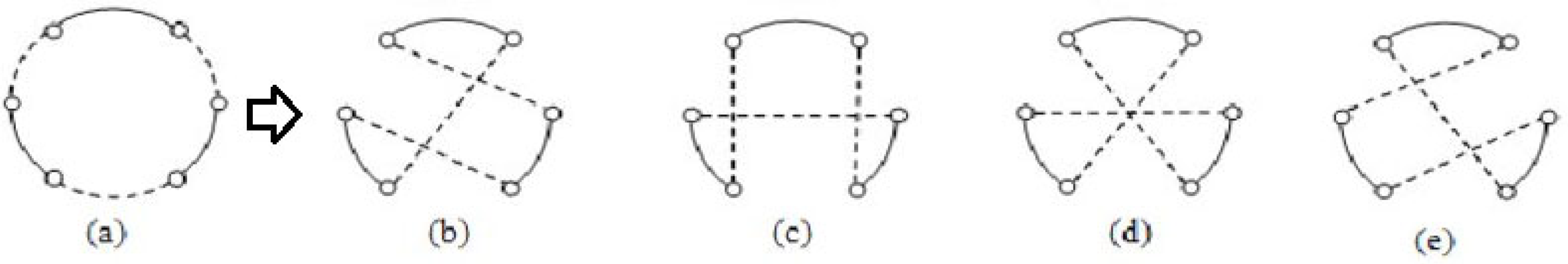
Figure 1 depicts an example of routes for the CVRP with three vehicles as follows.
 (A) 
Assumptions
(i)
Customer demand,   q i , is known 0 < qiQ;
(ii)
Limited vehicle capacity.
 (B) 
Variables and parameters
(i)
V: A set of customers is represented as V = {v0, v1, v2, …, vn} where n is the number of customers;
(ii)
cij: Transportation cost from nodes (customers) i to j;
(iii)
D: Length of the route (total distance that is travelled by the vehicle) should not surpass a particular defined constraint;
(iv)
Q: Capacity of each vehicle;
(v)
m: Number of vehicles;
(vi)
v0: Main distribution centre refers to the depot node where a tour starts and ends;
(vii)
K: Set of identical vehicles; K = {k0, k1, k2, …, km} is based on the main distribution centre, v0.
Dantzig and Ramser [1] proposed the first mathematical model for the CVRP ([6,39]) which is described below:
L e t   x i j k = 1   i f   v e h i c l e   k   g o e s   f r o m   i   t o   j 0   o t h e r w i s e
Minimize Z = i = 0 n j = 0 j i n k = 1 m c i j x i j   k    
Based on the following constraints:
k = 1 m j = 1 n x i j   k m ;   i = 0
i = 0 n x i j   k j = 0 n x j i   k = 0 ;   k K
k = 1 m i = 0 j i n x i j   k = 1 ;   j { 1 , , n }
k = 1 m j = 0 i j n x i j   k = 1 ;   i { 1 , , n }
j = 1 n x 0 j k 1 ;   k K  
i = 1 n x i 0 k 1 ;   k K
j = 1 n i = 0 i j n q j x i j k   Q ;   k K
k = 1 n i S j S i j x i j k | S | 1 ;   S V \ { 1 }
Equation (1) describes the objective functions used for minimizing the total distance travelled by a vehicle under constraint as shown in (2)–(8). Constraint (3) ensures that the number of vehicles entering a customer is the same as the number of vehicles leaving the same customer. Constraints (4) and (5) are applied for observing the customers who receive the service only once. On the other hand, Constraints (6) and (7) ensure that each vehicle that is used starts and ends at a depot and travels only once to offer its service. The main equation that is used for solving the CVRP problem is presented in (8) where it assigns the vehicle’s capacity for transporting different items. The sub-tour elimination constraints (9) guarantee that the solution contains no sub-tour.

3.2. Three-Opt Local Search Algorithm

A basic heuristic local search algorithm can be used for solving the TSP and network problems, like deleting the three edges of a tour or network and reconnecting them to three alternative edges for forming a network of all probable edges for determining the optimal tours. The researchers repeated this technique for different sets of three edges. It must be noted that there are many ways of connecting the nodes so that the tour can be restarted while also respecting the constraints of the problem [40]. In [32], all possible enhanced solutions by two-opt and three-opt are presented but we report only the possible solutions by three-opt in Figure 2 since we are applying three-opt in our proposed algorithm.

3.3. K-Nearest Neighbour (KNN) Algorithm

The K-nearest neighbour (KNN) algorithm is an effective technique that can be used for solving combinatorial optimization problems (COPs) like the CVRP. The KNNs are non-deterministic, i.e., they make random decisions which increases their robustness. This is a good technology that is used in the stochastic search for solving complex problems that need a bigger time space for determining the optimal solution. It is also seen to be a vital technique that is used for finding the optimal solutions. The KNN is regarded as a good technique that is used for solving hard problems with high computational complexity, particularly in the field of computer science. This technique has several applications like traffic optimization, the distribution of packages, and the selection of the tour where the aim of tour optimization for the VRP and TSP helps in decreasing the costs and visiting the locations with constraints ([41,42,43]). The steps of the KNN algorithm are as follows:
(i)
Load the training and testing data in the first step of the KNN algorithm;
(ii)
Choose a value of K (nearest data point);
(iii)
For every point included in the test data, the given steps must be implemented;
(a)
Using the Euclidean distance rule, estimate the distance between the test data and every row of the training data;
(b)
The distance values are sorted in ascending order;
(c)
The KNN algorithm selects the topmost K rows of the sorted values;
(d)
Assign a class to the test point depending on the most recurring class of rows.

3.4. Proposed Enhanced Ant Colony System (EACS) Algorithm

The ACS algorithm consists of four main steps—initialization, solution creation, local search, and pheromone update. The steps of the EACS algorithm are presented by proposing an enhancement mechanism based on the subpaths that achieve finding the best solutions for the proposed objectives. The enhancement is made in the step of building the solution which is characterized by the transition of the ant through the transitional equation that has a significant impact on achieving a balance between exploitation and exploration mechanisms. In the same context, this equation has been enhanced by using two mechanisms. The first one is related to the diversification by introducing a new term that supports the exploration mechanism of the transition equation from node to node. The second one is related to the intensification by selecting the best subpaths previously saved in a table that supports the exploitation mechanism for the transitional equation from node to subpath. The steps of our proposed EACS are as follows.
Step I (Initialization): Initialize the pheromone primary matrix, distance matrix, number of ants that are to be used, and control parameters—α, β, ρ, τ0, η i j , (Q ≥ 0). The total demand of items carried by each vehicle must not surpass the vehicle’s capacity, Q. η i j is the inverse of the distance between nodes i and j. The initial pheromone amount for every edge (i, j) depends on the following function: τ 0 = 1 l K N N where τ 0 > 0 represents the initial value describing the pheromone effect and l K N N refers to the cost generated by the KNN.
Step II: (i) (Solution creation): The transition rule equation used in the ACS algorithm was significant as it allowed the algorithm structure to enhance the solutions. This was attributed to the fact that based on the traditional formulation mentioned in Table 1, the ants move from one node to the other. Hence, it should be properly used for improving the transition and preventing any incorrect move to an unacceptable node since it could lead to a waste of effort and prove to be expensive. The transition rule is enhanced by using the two formulations described in Table 1.
After improving the transition rule, Step 1 implements the transition rule node by node for deriving new solutions. On the other hand, the second formulation was dependent on the movement between the node to subpaths for generating solutions. The first formulation is dependent on the subpaths because it helps in diversifying the solutions when travelling from one node to the next after the addition of a new term that supports the exploration mechanism since all terms in the initial transition rule support the exploitation mechanism implemented for this purpose. Then, all subpaths are saved after each iteration in the table while the repetitive subpaths are excluded for improving the diversification. Thereafter, the second formulation is applied in the intensification mechanism after determining the best solution while travelling from the node to the subpath. The best subpaths are stored after every iteration in different tables wherein all subpaths are utilized rather than depending on the nodes (i.e., the conventional formulation). The paths initiate at a particular node and stop at different specified nodes. The total distance and total pheromone concentration are calculated. Moreover, determine the amount of pheromone that is saved for every subpath of the path. Then, the transition rule is applied after they are considered as a single edge. The enhancement in the transition rule depends on the transition between the nodes or the transition to the subpath in the following manner (Equation (10)):
S = S C j   i f   h > a S P j   i f   h < a
Here, S C j   is the transition equation of node-by-node, S P j is the transition equation from node to subpath, h is the coefficient for utilizing the subpaths, and α 0 ,   1 is a random number. In the traditional transitional rule, a tour is carried out from one node to another wherein each ant successively adds new nodes until it visits all nodes. Here, if the ant k is present at node i, it moves to the next node, j, from the set of legal nodes, U (i.e., the set of unvisited nodes). The justification for suggesting this enhancement is because the ACS algorithm suffers from a lack of diversity so there is a need for improving the transitional rule which has derived from a set of terms with its associated coefficients that has been enhanced by most related studies ([44,45]) that used the terms to support exploitation. While this research work introduced a new term φ i l k   for this transitional rule in the enhanced ACS algorithm through which the passage of the same subpaths that were visited in previous solutions is avoided, this supports the exploration mechanism and, thus, the diversity is increased. The transitional rule became the following (Equation (11)):
S C j = a r g   m a x l U τ i l α η i l β ξ i l γ φ i l k δ   i f   q i Q J o t h e r w i s e
Here, φ i l k = 1 ψ i l k , ψ i l k   is the maximum number of continuously visited nodes from the beginning of the solution k that exist partly or completely on one of the recorded previous subpaths so that the more the number of nodes in the chosen subpath ψ i l k increases, the value of φ i l k decreases. Therefore, the probability of choosing it later decreases and the probability of exploring other subpaths then increases. Furthermore, (i, l) refers to the edge; l is the city that was not yet visited by ant k. If   q i Q , the exploitation mechanism was selected; however, if Q q i , the exploration was selected. J is the random variable that is specified based on the probability transition rule between different nodes p i j k [38] that was applied on the subpaths in the following manner (Equation (12)):
J : p i j k = τ i j α η i j β ξ i j γ φ i j k δ l U τ i l α η i l β ξ i l γ   i f   j U   0                                                                 o t h e r w i s e  
Here, τ i j is amount of pheromone on the edge E i j , η i j is the inverse of the distance between nodes i and j, ξij is the savings between nodes i and j, and α, β, γ, and δ are the control parameters. In the mechanism of building the solution by using the subpaths, we convert the terms of the transitional equation so that it depends on the subpaths and not on the edges as we select the best subpaths to build the solution sequentially. The transition rule based on subpaths is given as below (Equation (13)):
S P r = a r g   m a x l G τ P i l α η P i l β ξ P i l γ   i f   q i Q J r o t h e r w i s e
Here, J r is the random variable that is defined based on the probability of the transition rule from the node to a subpath p i r k which is applied according to the subpaths in the following manner (Equation (14)):
J r : p i r k = τ P i r α η P i r β ξ P i r γ l G τ P i l α η P i l β ξ P i l γ   i f   r G 0                                                                           o t h e r w i s e
Here, G represents the set of nodes of the subpaths that start at node i. Between the start and end nodes, these subpaths include many other unvisited nodes. These subpaths have a common feature where they start at one node and differ in other nodes and end at a different node while travelling between different paths.
Step II: (ii) (Local pheromone update): It includes the update of local pheromone to limit its concentration for exploring unused routes to produce different solutions and avoids the fall in a locally optimal, thus making the route less attractive for the next ants. Equation (15) shows the process of this stage.
τ i j t + 1 = 1 ρ · τ i j t + ρ τ 0
Here, ρ   ϵ   [ 0 ,   1 ] is a parameter, known as the evaporation coefficient, whose value is described in Table 2. τ 0 = ( L K N N ) 1 represents the primary pheromone level of edges and L K N N is the length of the tour generated by the KNN.
Step III: (Local search): In this section, the nodes are changed to enhance the route of all vehicles and, hence, to enhance the solutions that have been built by all ants through improving the quality of the solution of every ant. Alternatively, when utilizing the local search, the best local enhanced solutions might have a major chance to find the best solution. So, the local search is utilized for improving the solutions. Although this can be conducted in many ways, the most popular techniques include the use of two-opt and three-opt local search methods. In the two-opt method, two edges are eliminated from the tour and then the eliminated two edges are reconnected. The two edges can only be reconnected such that the validity of the tour is guaranteed and it is shorter. It is seen that the three-opt algorithm is operated similarly; however, rather than eliminating two edges, the algorithm removes three edges. This means that there are two techniques of reconnecting the three edges. In this study, we focused on using the large CVRP data, hence, we apply the three-opt technique for completing their subtour and k-opt was applied to various subpaths derived based on the experience of subpaths from the earlier iterations. This considered the installation of node 1 at last in every subpath. This ensures the enhancement of the best picture of the paths. In this phase, we apply the local search technique for improving the best solutions and thereby improving the best subpaths. This experience can help in successive iterations. This could be maximized after improving the subpaths where we can use them for global update.
Step IV: (Global pheromone update): A global update is carried out after every iteration wherein the pheromone values are updated based on the solution quality in the existing iteration. It can be performed by decreasing the pheromone values for all solutions using the evaporation procedure. This increases the pheromone value which helps in deriving the best solutions. On the other hand, in the EACS algorithm, the best elitist ants present in the iteration can lay the pheromone compound on the ribs where they travelled. A global updating rule may be described as follows (Equation (16)).
τ i j t + 1 = ρ τ i j t + Δ τ i j + Δ τ i j *
where
τ i j = μ = 1 σ 1 Δ τ i j μ , Δ τ i j μ = ( σ μ ) Q L μ   i f   t h e   μ - t h   b e s t   a n t   t r a v e l s   o n   e d g e   i , j 0   o t h e r w i s e  
a n d   Δ τ i j * = σ Q L *   i f   e d g e i , j   i s   p a r t   o f   t h e   b e s t   s o l u t i o n   f o u n d 0   o t h e r w i s e  
where μ = ranking index, Δ τ i j μ   refers to the increased trail level on the edge (i, j) that are affected by μ - t h best ant, L μ   = tour length of μ - t h best ant, Δ τ i j * represents the increase in the trail level on the edge (i, j) triggered by elitist ants, σ = no. of elitist ants, L * = tour length of the best solution, and t = iteration counter while ρ   ∈ (0, 1] is the parameter used for regulating the decrease in τ i j . The global update section collects all experience of the earlier iterations and updates the pheromone level of the best solution using another coefficient that differs from other coefficients used for the specific solutions that were not as effective as the elitist solutions. In the algorithm proposed in this study, the experience of the distinctive subpaths derived using the earlier iterations was retained for their later use. They could be used for developing solutions that were based on the experience of paths and helped in generating better results in less time. The pseudocode of the proposed EACS algorithm was presented as in Algorithm 1.
Algorithm 1: EACS algorithm
Symmetry 15 02020 i001

4. Results and Discussion

The results of the proposed EACS algorithm on benchmark CVRP data have been presented on a few statistical criteria. Furthermore, we compared the effectiveness of the proposed algorithm before and after the enhancement. We also compared the proposed algorithm with a state-of-the-art technique.

4.1. Statistical Criteria Used in the Study

The statistical criteria have included several statistical measures that have been used in this section to calculate the solutions for the CVRP instances that involve two types of solutions called best-known solution (BKS) and optimal solution (OPT). The statistical techniques used in the study include the calculation of the best solution (BS), average solution (AS), worst solution (WS), percentage of best gap (BG), percentage of average gap (AG), percentage of worst gap (WG), average time (AT), and standard deviation (SD) of 10 runs for each problem instance. In addition, the instances of the CVRP used in this study are taken from the CVRPLIB (http://vrp.galgos.inf.puc-rio.br/index.php/en/) accessed on 15 July 2023.

4.2. Parameter Tuning

The parameter tuning process is carried out for determining the best parameters that can help in improving the efficiency of the algorithm. It is noted that the grid search process is a simple optimization technique that carries out an exhaustive search process and manually derives a precise set of parameter regions for the classification technique. The benefit of the grid search technique is that the parameter settings are thoroughly created. For that, every dataset will be used to test all datasets [46]. Grid search has three steps which are given below.
(i)
Deriving the specific parameter settings depending on the specified cost limit. For example, the cost limit of five means the no. of specific settings for every parameter is five. Hence, for the despotic classifier with three parameters and a cost limit of five, the grid search process produces 5 × 5 × 5 = 125 mixtures of parameter settings.
(ii)
Assessing every specific parameter setting.
(iii)
Identification of the optimal parameter settings.
We report our parameters that are used in our proposed algorithm in Table 2.

4.3. Implementation of the EACS Algorithm on the CVRP Dataset

We have presented the results after applying the proposed EACS algorithm using the CVRP dataset. We have encoded our algorithm using MATLAB (R2018b (9.5.0.944444) on a 64 bit (win64) PC with Intel (R) Core (TM) i7-3770 CPU @ 3.40 GHz under MS Windows 10 and 8 GB RAM. We tested the application of the algorithm using different statistical measures; the best criterion was derived after solving the equations using the CVRP dataset wherein the lowest value was derived using the objective function of the CVRP model during repetition with the help of the proposed EACS algorithm. On the other hand, the worst criteria indicated the maximal value that could be derived from the objective function for the CVRP model during repetition with the help of the proposed EACS algorithm. One other criterion that was used included the average, i.e., mean of the objective function for the CVRP model during repetition with the help of the proposed EACS algorithm. Then, CPU time in seconds. Finally, SD denotes how far these values are far from the value in the centre. Moreover, to evaluate the solutions obtained through the proposed algorithm, Equation (19) was utilized to determine the percentage of gap (Gap) between the optimal solution and the best solution.
G a p = S C * C * × 100
Here, S is the obtained solution and C* is the OPT/BKS reported in the CVRPLIB. If the value of the gap is zero, then the solution is optimal; if the gap is close to zero, then it is a good solution; and if the gap is away from zero, then it is not a good solution. For example, as for the instance CMT1 from the CVRP dataset, this instance has an optimal solution in the CVRP dataset and its value is 524.61. When implementing our proposed EACS algorithm on this instance, we obtained BS value 524.61 after 10 runs. To evaluate this solution, we find the gap as follows:
G a p = 524.61 524.61 524.61 × 100 = 0.00
Table 3 shows the results of the EACS algorithm in the case of a CVRP dataset, called CMT, which contains 14 instances, out of which 13 instances have OPT and 1 instance has BKS. The results show that the algorithm could obtain 12 OPTS out of 13 OPTS and 1 BKS out of 1 BKS. The average of the best solutions is 983.54 while the average of solutions in CVRPLIB is 976.03; that means the average percentage of the best gap is 0.72 with an average SD of 21.91 and the average time is 249.53 s, which is a reasonable time.
The results of the proposed EACS algorithm on the case “Set P” of CVRP dataset have presented in Table 4, which has 23 instances, and the type of solutions is OPT. The results show that the EACS algorithm obtained 21 OPTS out of 23 OPTS and the average of BS is 591.48 which is the same as the average of solutions in CVRP. That means the average of the BG is 0.52, with the average SD being 8.88 and the average time being 157.61 s, which is a reasonable time.

4.4. Evaluating the Effectiveness of Our EACS Algorithm

We have assessed the effectiveness of the ACS algorithm after its enhancement with the help of the subpath. This assessment was carried out in the following manner.

4.4.1. Comparison between the ACS and EACS Algorithms

We have compared the performance between ACS and EACS algorithms based on the gap (accuracy) mentioned in Equation (19). Table 5 shows the comparative results.
The comparison was confirmed in the previous section that relied on evaluation metrics for the EACS algorithm, has outstanding performance, and is superior to ACS algorithm. This is reflected positively to optimize the solutions of the CVRP instances within a reasonable computational time. For example, the Bgs of the instances CMT3, CMT4, CMT5, CMT7, CMT8, CMT10, CMT11, and CMT12 are 1.67, 1.54, 2.31, 1.69, 1.28, 2.07, 10.62, and 2.58, respectively, using the ACS algorithm. These Bgs have been reduced to 0.00, 0.00, 0.00, 0.00, 0.00, 0.00, 10.09, and 0.00, respectively, using the EACS algorithm. For the average of AT for all “CMT” instances, the ACS algorithm takes 328.84 s whereas the EACS algorithm takes 249.53 s.
Furthermore, a comparison between ACS and EACS algorithms was conducted on the CVRP “P-n-k” case and is reported in Table 6. The exploration issue in the ACS algorithm had a negative impact on its efficiency, robustness, and strong convergence so the performance negatively affected the obtained results. For example, the BG of the instances P-n16-k8, P-n19-k2, P-n20-k2, P-n22-k8, P-n23-k8, P-n60-k15, P-n65-k10, and P-n70-k10 were 22.89, 11.32, 10.19, 7.63, 19.85, 12.81, 5.68, and 8.83, respectively, using the ACS algorithm. Conversely, the EACS algorithm dealt with the exploration issue by using subpaths and thus it was able to increase the diversity, which reflected positively on the performance of the algorithm and thus achieved 21 OPTS out of 23 OPTS of the “P-n-k” instances from CVRP dataset. In terms of implementation time, the traditional algorithm ACS found solutions for these instances within 189.44 s; the EACS algorithm resolved those cases within 114.132 s.

4.4.2. Comparison between ACS and EACS Algorithms Based on the Efficiency Criteria

For comparing the efficiency of the algorithms, one of the three formulations is used which are given below [47].
(i)
Minimum number of times\iteration to find new solutions given by the following formula:
λmin = mins {λs + 1}
(ii)
Mean number of times\iteration to find new solutions given by the following formula:
λ mean = S = 1 S 1 λ s + 1 S
(iii)
Maximum number of times\iteration to find new solutions given by the following formula:
λmax = maxs {λs + 1}
Here, λ = time (seconds) or no. of iterations carried out for determining new solutions; λs+1 = time (seconds) or no. of iterations conducted for determining new solutions that start from a solution number, s; S = solution index; S + 1 = new solution index. We have used the first formula, i.e., Equation (20), to compare the efficiency of the algorithms. So, the algorithm is more robust if λmin is less than other algorithms. Table 7 shows the comparison between the ACS and EACS algorithms based on the efficiency criteria on the “CMT” case.
Based on the results reported in Table 7, the EACS algorithm gives lower values for the efficiency measure, which means that it discovers a new solution in a shorter time, unlike the traditional ACS algorithm which gives high values for an efficiency measure, especially if the size of the instance (n) is large. For example, for the instances CMT4, CMT5, and CMT13 of sizes 150, 199, and 120, respectively, the efficiency rates of the ACS algorithm are 86.00, 98.33, and 93.00, respectively, while the efficiency rates of the EACS algorithm are 29.00, 35.20, and 29.75, respectively.
Another comparison between ACS and EACS algorithms using the evaluation metrics has been presented in Table 8 on “P-n-k” data of CVRP.
The results in Table 8 show that the enhanced EACS algorithm has an outstanding performance compared to the traditional ACS algorithm based on the efficiency criteria. The efficiency results of the ACS algorithm are higher than that of those by the EACS algorithm. For example, the results of the instances P-n55-k15, P-n60-k10, P-n60-k15, P-n65-k10, and P-n70-k10 using the ACS algorithm are 58.80, 36.00, 40.50, 65.25 and 52.67, respectively, while the results of those instances using the EACS algorithm are 9.50, 11.00, 20.20, 10.67, and 7.50, respectively.

4.4.3. Comparison of EACS Algorithm with a State-of-the-Art Algorithm

In this section, our EACS algorithm is compared with one of the state-of-the-art methods that solved the CVRP. In [47], a simulated annealing algorithm based on the population (PSA) was proposed to solve the CVRP and was implemented on some well-known instances from the CVRP dataset. Table 9 reports the results of this comparison.
Notably, the values in boldfaces are obtained by our proposed EACS algorithm that indicate better results than those obtained by the PSA [47]. Figure 3, Figure 4, Figure 5 and Figure 6 show the no. of OPT obtained by our EACS algorithm and the PSA algorithm [47] on “Sets A, B, P, and E” datasets from the CVRP.

5. Theoretical Analysis and Critical Explanation for the Performance of the Proposed EACS Algorithm

Many earlier studies showed that the metaheuristic algorithms are very effective in handling the NP-hard problems. Hence, in this study, we proposed an EACS algorithm belonging to the swarm intelligence (SI) category, which is a class of metaheuristic algorithms. The no free lunch (NFL) theorem [48] used in the optimization field states that no single algorithm displays a good performance while solving all problems. Moreover, this performance can also be poor in a few instances. Hence, we have proposed an enhanced algorithm that would show an enhanced performance on a specific problem; however, it would not provide a comprehensive solution for all problems.
For achieving an efficient performance of this proposed algorithm, the metaheuristic algorithms must address some issues like lack of an exploration mechanism, stagnation, and parameter tuning. All these issues have been addressed in this study. Furthermore, studies in the literature have succeeded in improving the intensification (exploitation) of the ACS algorithm by the experience of subpaths [23]. However, the ACS algorithm is suffering from an exploration issue; therefore, this study has considered this issue by enhancing the traditional transition rule in the ACS algorithm by using the subpaths to support the exploration mechanism in the EACS algorithm where all subpaths are stored after finishing every iteration in a table to exclude repeated subpaths for achieving diversification. To verify that our proposed algorithm has a good contribution, the performance was evaluated using evaluation metrics that included efficiency and gap. The proposed algorithm showed an enhanced efficiency as the convergence was increased to optimal solutions within a reasonable computation time for the CMT6, as shown in Figure 7, Figure 8, Figure 9 and Figure 10.

Statistical Analysis

In this section, we have presented a statistical analysis of all findings displayed by the EACS and the ACS algorithms where they used the p-value for rejecting the null hypothesis as follows. The statistical analysis related to comparison between the best solutions obtained by the ACS and EACS algorithms that have solved some of the instances from the CVRP dataset. The different hypotheses consist of the null hypothesis, which refers to the average of the best solutions acquired by the ACS algorithm. This was seen to be equal to the mean of all best solutions derived using the EACS algorithm. Hypothesis 2 refers to the alternative hypothesis, which is seen to be the mean best solution that is derived with the help of the ACS algorithm. This was not equal to the mean of the best solutions acquired using the EACS algorithm. Table 10 presents the statistical analysis of the paired samples.
As shown in Table 10, the p-value of the null hypothesis was less than 0.05 in the 95% confidence interval, hence, it was rejected. This indicated that there was strong evidence indicating that the above solutions were different. Owing to its positive value, the solutions derived using the ACS algorithm were worse compared to the solutions derived using the EACS algorithm. On the other hand, the Wilcoxon signed-rank test was used for statistically analyzing the performance of the proposed EACS algorithm and the algorithm PSA that was proposed in [49] as follows:
No difference was noted between the average value obtained using the PSA and the proposed EACS algorithms for the null hypothesis. On the other hand, differences were noted in the mean value calculated using the proposed EACS and PSA algorithms in the case of the alternative hypothesis. The results of this test have been presented in Table 11 and Table 12.
The test statistics have been presented in Table 12.
As shown in Table 11 and Table 12, the test value was seen to be −4.82 while the confidence level was 0.00, which was less than 0.05. Hence, the researchers have rejected the null hypothesis and accepted the alternative hypothesis. Though the comparative study showed a better performance of our EACS compared to the enhanced simulated annealing algorithm, our proposed algorithm could not find an optimal solution for all problem instances.

6. Conclusions

Despite the metaheuristic algorithms’ success, balancing the smart mechanisms owned by these algorithms represented in exploitation and exploration is considered a challenge for most of these algorithms. Therefore, this research work has addressed the exploration issue in the ACS algorithm by using subpaths to avoid generating the same solutions, thus leveraging the diversity of generating solutions to find better solutions with less route distance in a reasonable time. The performance evaluation results of the EACS algorithm have shown that the EACS algorithm is better than the ACS algorithm based on the evaluation metrics efficiency and powerful convergence in addition to being better than that based on the gap (accuracy) by using Equation (18). In this study, we also compared the EACS algorithm with a state-of-the-art technique and noted that our proposed EACS algorithm showed a better performance compared to the enhanced simulated annealing algorithm. The enhanced simulated annealing algorithm yielded 29 optimal solutions out of the 61 optimal solutions whereas the proposed EACS algorithm yielded 57 out of the 61 optimal solutions.
Though the comparative study showed a better performance of our EACS compared to the enhanced simulated annealing algorithm (PSA), our proposed algorithm could not find optimal solution for all problem instances. So, other metaheuristic algorithms, like genetic algorithms, tabu search [50], and/or combination of them can show better performance of the algorithm. Furthermore, the proposed EACS algorithm can be used for solving many healthcare-related combinatorial optimization problems like the nurse scheduling problem (NSP) within a shorter computational time.

Author Contributions

Conceptualization, Z.H.A. and M.L.M.; Methodology, A.S.H. and H.H.; Software M.L.M.; Validation A.S.H. and M.L.M.; Investigation, Z.H.A., A.S.H. and H.H.; Resources, M.L.M. and H.H.; Data curation, A.S.H.; Writing—original draft, A.S.H.; Writing—review & editing, Z.H.A. and H.H.; Supervision Z.H.A.; Project administration, H.H.; Funding acquisition, Z.H.A. All authors have read and agreed to the published version of the manuscript.

Funding

This research was funded by the Deanship of Scientific Research at Imam Mohammad Ibn Saud Islamic University (IMSIU) (grant number IMSIU-RP23030).

Data Availability Statement

The dataset used to support the findings of this study is available in ORLibrary.

Acknowledgments

The authors express their gratitude for the financial support provided by the Deanship of Scientific Research at Imam Mohammad Ibn Saud Islamic University (IMSIU).

Conflicts of Interest

The authors declare no conflict of interest.

References

  1. Dantzig, G.B.; Ramser, J.H. The Truck Dispatching Problem. Manag. Sci. 1959, 6, 80–91. [Google Scholar] [CrossRef]
  2. Contardo, C.; Martinelli, R. A new exact algorithm for the multi-depot vehicle routing problem under capacity and route length constraints. Discret. Optim. 2014, 12, 129–146. [Google Scholar] [CrossRef]
  3. Hameed, A.S.; Aboobaider, B.M.; Choon, N.H.; Mutar, M.L.; Bilal, W.H. A comparative study between the branch and cut algorithm and ant colony algorithm to solve the electric meter reader problem in rural areas. Opcion 2018, 34, 1525–1539. [Google Scholar]
  4. Dorigo, M.; Maniezzo, V.; Colorni, A. Ant system: An autocatalytic optimizing process. In Technical Report 91-016; Politecnico di Milano: Milano, Italy, 1991; pp. 1–21. [Google Scholar]
  5. Bell, J.E.; McMullen, P.R. Ant colony optimization techniques for the vehicle routing problem. Adv. Eng. Inform. 2004, 18, 41–48. [Google Scholar] [CrossRef]
  6. Stodola, P.; Mazal, J.; Podhorec, M.; Litvaj, O. Using the Ant Colony Optimization algorithm for the Capacitated Vehicle Routing Problem. In Proceedings of the 16th International Conference on Mechatronics-Mechatronika (ME), Brno, Czech Republic, 3–5 December 2014; pp. 503–510. [Google Scholar]
  7. Necula, R.; Breaban, M.; Raschip, M. Tackling Dynamic Vehicle Routing Problem with Time Windows by means of ant colony system. In Proceedings of the 2017 IEEE Congress on Evolutionary Computation (CEC), San Sebastian, Spain, 5–8 June 2017; pp. 2480–2487. [Google Scholar]
  8. Gallotti, R.; Chialvo, D.R. How ants move: Individual and collective scaling properties. J. R. Soc. Interface 2018, 15, 20180223. [Google Scholar] [CrossRef]
  9. Pérez-Delgado, M.-L. Color quantization with Particle swarm optimization and artificial ants. Soft Comput. 2020, 24, 4545–4573. [Google Scholar] [CrossRef]
  10. Mutar, M.L.; Burhanuddin, M.A.; Hameed, A.S.; Yusof, N.; Mutashar, H.J. An efficient improvement of ant colony system algorithm for handling capacity vehicle routing problem. Int. J. Ind. Eng. Comput. 2020, 11, 549–564. [Google Scholar] [CrossRef]
  11. Jabbar, A.M.; Sagban, R.; Ku-Mahamud, K.R. Balancing exploration and exploitation in acs algorithms for data clustering. J. Theor. Appl. Inf. Technol. 2019, 97, 4320–4333. [Google Scholar]
  12. Lloyd, H.; Amos, M. Solving sudoku with ant colony optimization. IEEE Trans. Games 2020, 12, 302–311. [Google Scholar] [CrossRef]
  13. Altabeeb, A.M.; Mohsen, A.M.; Ghallab, A. An improved hybrid firefly algorithm for capacitated vehicle routing problem. Appl. Soft Comput. 2019, 84, 105728. [Google Scholar] [CrossRef]
  14. İlhan, İ. An improved simulated annealing algorithm with crossover operator for capacitated vehicle routing problem. Swarm Evol. Comput. 2021, 64, 100911. [Google Scholar] [CrossRef]
  15. Zhu, J. Solving Capacitated Vehicle Routing Problem by an Improved Genetic Algorithm with Fuzzy C-Means Clustering. Sci. Program. 2022, 2022, 8514660. [Google Scholar] [CrossRef]
  16. Ahmed, Z.H.; Ahmed, Z.H.; Hameed, A.S.; Hameed, A.S.; Mutar, M.L.; Mutar, M.L. Hybrid Genetic Algorithms for the Asymmetric Distance-Constrained Vehicle Routing Problem. Math. Probl. Eng. 2022, 2022, 2435002. [Google Scholar] [CrossRef]
  17. Ahmed, Z.H.; Al-Otaibi, N.; Al-Tameem, A.; Saudagar, A.K.J. Genetic Crossover Operators for the Capacitated Vehicle Routing Problem. Comput. Mater. Contin. 2023, 74, 1575–1605. [Google Scholar] [CrossRef]
  18. Ahmed, Z.H.; Maleki, F.; Yousefikhoshbakht, M.; Haron, H. Solving the vehicle routing problem with time windows using modified football game algorithm. Egypt. Inform. J. 2023, 24, 100403. [Google Scholar] [CrossRef]
  19. Wu, W.; Tian, Y.; Jin, T. A label based ant colony algorithm for heterogeneous vehicle routing with mixed backhaul. Appl. Soft Comput. 2016, 47, 224–234. [Google Scholar] [CrossRef]
  20. Kuo, R.J.; Zulvia, F.E. Hybrid genetic ant colony optimization algorithm for capacitated vehicle routing problem with fuzzy demand—A case study on garbage collection system. In Proceedings of the 2017 4th International Conference on Industrial Engineering and Applications (ICIEA), Nagoya, Japan, 21–23 April 2017; pp. 244–248. [Google Scholar]
  21. Zhai, Y.; Xiang, Z. Overview of Pheromone Control Method based on Ant Colony Algorithm in Wireless Communication. In Proceedings of the 2019 7th International Conference on Information, Communication and Networks (ICICN), Macau, China, 24–26 April 2019; pp. 1–5. [Google Scholar]
  22. Skinderowicz, R. An improved Ant Colony System for the Sequential Ordering Problem. Comput. Oper. Res. 2017, 86, 1–17. [Google Scholar] [CrossRef]
  23. Dorigo, M.; Stützle, T. Ant colony optimization: Overview and recent advances. In Handbook of Metaheuristics; Gendreau, M., Potvin, J.Y., Eds.; International Series in Operations Research & Management Science; Springer: Cham, Switzerland, 2010; Volume 272. [Google Scholar] [CrossRef]
  24. Cheong, P.Y.; Aggarwal, D.; Hanne, T.; Dornberger, R. Variation of ant colony optimization parameters for solving the travelling salesman problem. In Proceedings of the 2017 IEEE 4th International Conference on Soft Computing & Machine Intelligence (ISCMI), Port Louis, Mauritius, 23–24 November 2017; pp. 60–65. [Google Scholar]
  25. Akhtar, A. Evolution of Ant Colony Optimization Algorithm—A Brief Literature Review. arXiv 2019, arXiv:1908.08007. [Google Scholar] [CrossRef]
  26. Colorni, A.; Dorigo, M.; Maniezzo, V. Distributed optimization by ant colonies. In Proceedings of the European Conference on Artificial Life, ECAL’91, Paris, France; Varela, F., Bourgine, P., Eds.; Elsevier Publishing: Amsterdam, The Netherlands, 1991; pp. 134–142. [Google Scholar]
  27. Yu, B.; Yang, Z.-Z.; Yao, B. An improved ant colony optimization for vehicle routing problem. Eur. J. Oper. Res. 2009, 196, 171–176. [Google Scholar] [CrossRef]
  28. Matos, A.C.; Oliveira, R.C. An Experimental Study of the Ant Colony System for the Period Vehicle Routing Problem. In Ant Colony Optimization and Swarm Intelligence; Dorigo, M., Birattari, M., Blum, C., Gambardella, L.M., Mondada, F., Stützle, T., Eds.; ANTS 2004. Lecture Notes in Computer Science; Springer: Berlin/Heidelberg, Germany, 2004; Volume 3172. [Google Scholar] [CrossRef]
  29. Oonsrikaw, Y.; Thammano, A. Enhanced Ant Colony Optimization with Local Search. In Proceedings of the 2018 IEEE/ACIS 17th International Conference on Computer and Information Science (ICIS), Singapore, 6–8 June 2018; pp. 291–296. [Google Scholar]
  30. Bullnheimer, B.; Hartl, R.; Strauss, C. An improved Ant System algorithm for theVehicle Routing Problem. Ann. Oper. Res. 1999, 89, 319–328. [Google Scholar] [CrossRef]
  31. Kheirkhahzadeh, M.; Barforoush, A.A. A hybrid algorithm for the vehicle routing problem. In Proceedings of the 2009 IEEE Congress on Evolutionary Computation (CEC), Trondheim, Norway, 18–21 May 2009; pp. 1791–1798. [Google Scholar]
  32. Gianluca; Tan, W.F.; Lee, L.S.; Majid, Z.A.; Seow, H.V. Ant Colony Optimization for Capacitated Vehicle Routing Problem. J. Comput. Sci. 2012, 8, 846–852. [Google Scholar] [CrossRef]
  33. Stützle, T.; Hoos, H.H. MAX–MIN Ant System. Futur. Gener. Comput. Syst. 2000, 16, 889–914. [Google Scholar] [CrossRef]
  34. Dorigo, M.; Birattari, M.; Stutzle, T. Ant colony optimization. IEEE Comput. Intell. Mag. 2006, 1, 28–39. [Google Scholar] [CrossRef]
  35. Sankar, K.; Krishnamoorthy, K. Ant Colony algorithm for routing problem using rule-mining. In Proceedings of the 2010 IEEE International Conference on Computational Intelligence and Computing Research (ICCIC), Coimbatore, India, 28–29 December 2010; pp. 1–8. [Google Scholar]
  36. Tang, J.; Guan, J.; Yu, Y.; Chen, J. Beam Search Combined With MAX-MIN Ant Systems and Benchmarking Data Tests for Weighted Vehicle Routing Problem. IEEE Trans. Autom. Sci. Eng. 2014, 11, 1097–1109. [Google Scholar] [CrossRef]
  37. Li, X.; Wang, Y. Scheduling Batch Processing Machine Using Max–Min Ant System Algorithm Improved by a Local Search Method. Math. Probl. Eng. 2018, 2018, 3124182. [Google Scholar] [CrossRef]
  38. Xia, M. A modified Ant Colony Algorithm with local search for capacitated vehicle routing problem. In Proceedings of the 2009 Asia-Pacific Conference on Computational Intelligence and Industrial Applications (PACIIA 2009), Wuhan, China, 19–20 December 2009; pp. 84–87. [Google Scholar]
  39. Janjarassuk, U.; Masuchun, R. An ant colony optimization method for the capacitated vehicle routing problem with stochastic demands. In Proceedings of the 2016 International Computer Science and Engineering Conference (ICSEC), Chiang Mai, Thailand, 14–17 December 2016; pp. 1–5. [Google Scholar]
  40. Mazidi, A.; Fakhrahmad, M.; Sadreddini, M. A Meta-heuristic approach to CVRP Problem: Local search optimization based on GA and ant colony. J. Adv. Comput. Res. 2016, 7, 1–22. [Google Scholar]
  41. Schuijbroek, J.; Hampshire, R.; van Hoeve, W.-J. Inventory rebalancing and vehicle routing in bike sharing systems. Eur. J. Oper. Res. 2017, 257, 992–1004. [Google Scholar] [CrossRef]
  42. Abdul Khalid, N.E.; Ibrahim, S.; Haniff, P.N.M.M. MRI brain abnormalities segmentation using K-nearest neighbors (k-NN). Int. J. Comput. Sci. Eng. 2011, 3, 980–990. [Google Scholar]
  43. Mohammed, M.A.; Ghani, M.K.A.; Hamed, R.I.; Mostafa, S.A.; Ibrahim, D.A.; Jameel, H.K.; Alallah, A.H. Solving vehicle routing problem by using improved K-nearest neighbor algorithm for best solution. J. Comput. Sci. 2017, 21, 232–240. [Google Scholar] [CrossRef]
  44. Dorigo, M.; Gambardella, L. Ant colony system: A cooperative learning approach to the traveling salesman problem. IEEE Trans. Evol. Comput. 1997, 1, 53–66. [Google Scholar] [CrossRef]
  45. Hsu, C.-C.; Hou, R.-Y.; Wang, W.-Y. Path Planning for Mobile Robots Based on Improved Ant Colony Optimization. In Proceedings of the 2013 IEEE International Conference on Systems, Man and Cybernetics (SMC 2013), Manchester, UK, 13–16 October 2013; pp. 2777–2782. [Google Scholar]
  46. Tantithamthavorn, C.; McIntosh, S.; Hassan, A.E.; Matsumoto, K. The Impact of Automated Parameter Optimization on Defect Prediction Models. IEEE Trans. Softw. Eng. 2019, 45, 683–711. [Google Scholar] [CrossRef]
  47. Tavakkoli-Moghaddam, R.; Raziei, Z.; Tabrizian, S. Performance analysis of meta-heuristic algorithms for a quadratic assignment problem. arXiv 2020, arXiv:2007.14885. [Google Scholar] [CrossRef]
  48. Ilhan, I. A population based simulated annealing algorithm for capacitated vehicle routing problem. Turk. J. Electr. Eng. Comput. Sci. 2020, 28, 1217–1235. [Google Scholar] [CrossRef]
  49. Wolpert, D.H.; Macready, W.G. No free lunch theorems for optimization. IEEE Trans. Evol. Comput. 1997, 1, 67–82. [Google Scholar] [CrossRef]
  50. Ahmed, Z.H.; Yousefikhoshbakht, M. An improved tabu search algorithm for solving heterogeneous fixed fleet open vehicle routing problem with time windows. Alex. Eng. J. 2022, 64, 349–363. [Google Scholar] [CrossRef]
Figure 1. Routes for the CVRP with three vehicles.
Symmetry 15 02020 g001
Figure 2. (a) The original Hamiltonian cycle, (be) All other possible Hamiltonian cycles using three-opt search.
Symmetry 15 02020 g002
Figure 3. No. of OPT obtained by EACS and PSA on the “Set A” case.
Symmetry 15 02020 g003
Figure 4. No. of OPT obtained by EACS and PSA on the “Set B” case.
Symmetry 15 02020 g004
Figure 5. No. of OPT obtained by EACS and PSA on the “Set P” case.
Symmetry 15 02020 g005
Figure 6. No. of OPT obtained by EACS and PSA on the “Set E” case.
Symmetry 15 02020 g006
Figure 7. Strong convergence rate of best, worst, and average solutions by the EACS algorithm to solve the instance of CMT6.
Symmetry 15 02020 g007
Figure 8. Strong convergence rate of the best, worst, and average solutions by the ACS algorithm to solve the instance of CMT6.
Symmetry 15 02020 g008
Figure 9. Time efficiency of strong convergence by EACS algorithm to solve the instance of CMT6.
Symmetry 15 02020 g009
Figure 10. Time efficiency of strong convergence by ACS algorithm to solve the instance of CMT6.
Symmetry 15 02020 g010
Table 1. Transitional rules before and after enhancement.
Traditional Formulation ([38,39])Formulation after the Enhancement
S j = a r g   m a x l U τ i l α η i l β ,   i f   q i Q p i j k = τ i j α η i j β l U τ i l α η i l β     j U ,   o t h e r w i s e 1-  S C j = a r g   m a x l U τ i l α η i l β ξ i l γ φ i l k δ ,   i f   q i Q p i j k = τ i j α η i j β ξ i j γ φ i j k δ l U τ i l α η i l β ξ i l γ   j U ,   o t h e r w i s e
2-  S P r = a r g   m a x l G τ P i l α η P i l β ξ P i l γ ,   i f   q i Q p i r k = τ P i r α η P i r β ξ P i r γ l G τ P i l α η P i l β ξ P i l γ   r G ,   o t h e r w i s e
Table 2. Parameter settings used in our algorithm.
ParametersValue
β 2
q 0 0.90
α 2
ρ 0.90
τ 0 L K N N 1
γ 2
σ 5
No. of iterations, N1000
Q As in the CVRPLIB
No. of vehicles, mAs in the CVRPLIB
No. of ants, n = mAs in the CVRPLIB
Table 3. Results of the EACS algorithm on the “CMT” case.
No.InstanceSolution in CVRPLIBType of SolutionBSWSASBGWGAGSDAT(s)
1CMT1524.61OPT524.61594.23531.570.0013.271.3322.0125.44
2CMT2835.26OPT835.26940.47845.780.0012.601.2633.2749.83
3CMT3826.14OPT826.14969.38840.460.0017.341.7345.30117.17
4CMT41028.42OPT1028.421028.421028.420.000.000.000.00256.98
5CMT51291.29OPT1291.291291.291291.290.000.000.000.00802.21
6CMT6555.43OPT555.43595.82563.030.007.271.3716.0627.93
7CMT7909.68OPT909.67909.67909.670.000.000.000.0060.33
8CMT8865.94OPT865.94865.94865.940.000.000.000.00107.81
9CMT91162.55OPT1162.551302.091188.490.0012.002.2354.88281.36
10CMT101395.85OPT1395.851706.141426.880.0022.232.2298.12548.20
11CMT111042.11OPT1147.271174.831159.5310.0912.7411.278.64653.23
12CMT12819.56OPT819.56909.57828.560.0010.981.1028.47230.60
13CMT131541.14No1541.141541.141541.140.000.000.000.00209.67
14CMT14866.37OPT866.37866.37866.370.000.000.000.00122.64
Average976.03 983.541049.67991.940.727.741.6121.91249.53
Table 4. Results of the EACS algorithm on the “Set P” case.
No.InstanceSolution in CVRPLIBType of SolutionBSWSASBGWGAGSDAT(s)
1P-n16-k8450OPT450450450.000.000.000.000.002.54
2P-n19-k2212OPT212224213.200.005.660.573.7916.85
3P-n20-k2216OPT216216216.000.000.000.000.0012.88
4P-n21-k2211OPT211218211.700.003.320.332.2120.47
5P-n22-k2216OPT216226217.700.004.630.793.6515.86
6P-n22-k8603OPT603603603.000.000.000.000.001398.34
7P-n23-k8529OPT529529529.000.000.000.000.0021.37
8P-n40-k5458OPT458482460.400.005.240.527.5912.75
9P-n45-k5510OPT510560515.000.009.800.9815.8132.31
10P-n50-k7554OPT554603571.200.008.843.1022.5134.30
11P-n50-k8631OPT631662634.100.004.910.499.8032.64
12P-n50-k10696OPT719741735.303.306.475.656.53431.94
13P-n51-k10741OPT741788745.700.006.340.6314.8648.09
14P-n55-k7568OPT568568568.000.000.000.000.0024.99
15P-n55-k10694OPT694694694.000.000.000.000.0026.98
16P-n55-k15989OPT989989989.000.000.000.000.0032.81
17P-n60-k10744OPT744799754.500.007.391.4122.1742.91
18P-n60-k15968OPT9681025973.700.005.890.5918.0361.54
19P-n65-k10792OPT792874807.900.0010.352.0133.5464.51
20P-n70-k10827OPT898915908.108.5910.649.816.711002.21
21P-n76-k4593OPT593593593.000.000.000.000.0074.70
22P-n76-k5627OPT627718644.500.0014.512.7936.93108.62
23P-n101-k4681OPT681681681.000.000.000.000.00105.45
Average587.39 591.48615.57596.350.524.521.298.88157.61
Table 5. Comparison between ACS and EACS algorithms on the “CMT” case.
InstanceSolution in CVRPLIBACS AlgorithmEACS Algorithm
BSBGAT(s)BSBGAT(s)
CMT1524.61524.610.00114.04524.610.0025.44
CMT2835.26838.180.3588.91835.260.0049.83
CMT3826.14839.921.67282.87826.140.00117.17
CMT41028.421044.291.54546.611028.420.00256.98
CMT51291.291321.072.31863.891291.290.00802.21
CMT6555.43560.240.8744.43555.430.0027.93
CMT7909.68925.091.69107.97909.670.0060.33
CMT8865.94877.001.28139.46865.940.00107.81
CMT91162.551167.040.39334.981162.550.00281.36
CMT101395.851424.702.07688.651395.850.00548.20
CMT111042.111152.8010.62750.101147.2710.09653.23
CMT12819.56840.722.58224.36819.560.00230.60
CMT131541.141551.350.66301.191541.140.00209.67
CMT14866.37868.400.23116.27866.370.00122.64
Average995.391.88328.84983.540.72249.53
Table 6. Comparison between ACS and EACS algorithms on “P-n-k” case.
InstanceSolution in CVRPLIBACS AlgorithmEACS Algorithm
BS BGAT(s) BSBGAT(s)
P-n16-k845055322.8912.704500.002.54
P-n19-k221223611.3255.802120.0016.85
P-n20-k221623810.1928.532160.0012.88
P-n21-k22112110.0090.572110.0020.47
P-n22-k22162160.0078.172160.0015.86
P-n22-k86036497.631241.346030.00398.34
P-n23-k852963419.8534.355290.0021.37
P-n40-k54584743.4916.224580.0012.75
P-n45-k55105232.5536.305100.0032.31
P-n50-k75545794.5147.265540.0034.30
P-n50-k86316777.2977.336310.0032.64
P-n50-k1069678312.50511.587193.30431.94
P-n51-k107418028.2369.187410.0048.09
P-n55-k75685934.4043.085680.0024.99
P-n55-k106947426.9238.526940.0026.98
P-n55-k15989109911.1242.549890.0032.81
P-n60-k1074483011.5651.827440.0042.91
P-n60-k15968109212.8185.339680.0061.54
P-n65-k107928375.6863.577920.0064.51
P-n70-k10 827 9008.831218.178988.591002.21
P-n76-k45936031.69141.345930.0074.70
P-n76-k56276493.51168.356270.00108.62
P-n101-k46816911.47205.136810.00105.45
Average635.267.76189.44591.480.52114.13
Table 7. Comparison between ACS and EACS algorithms using efficiency criteria on the “CMT” case.
InstanceEfficiency Criteria
ACSEACS
CMT156.4030.50
CMT268.5024.88
CMT374.5029.13
CMT486.0029.00
CMT598.3335.20
CMT665.0025.38
CMT773.0056.40
CMT884.7516.67
CMT986.5052.00
CMT1095.0057.00
CMT1178.334.43
CMT1296.5072.75
CMT1393.0029.75
CMT1476.3332.20
Table 8. Comparison between ACS and EACS algorithms using efficiency criteria on the “P-n-k” case.
InstanceEfficiency Criteria
ACSEACS
P-n16-k876.0036.00
P-n19-k274.7529.75
P-n20-k225.133.50
P-n21-k247.006.33
P-n22-k245.0012.50
P-n22-k862.6710.50
P-n23-k825.005.50
P-n40-k533.0014.50
P-n45-k524.006.25
P-n50-k739.6724.80
P-n50-k836.7515.60
P-n50-k1032.6014.00
P-n51-k1042.0022.00
P-n55-k748.6738.53
P-n55-k1040.0018.00
P-n55-k1558.809.50
P-n60-k1036.0011.00
P-n60-k1540.5020.20
P-n65-k1065.2510.67
P-n70-k1052.677.50
P-n76-k448.5031.20
P-n76-k557.0034.75
P-n101-k455.8037.33
P-n16-k876.0036.00
Table 9. Comparison between EACS algorithm and PSA [47].
No.InstanceSolution in CVRPLIBBest Solutions by
PSAEACS
1A-n32-k5784784784
2A-n33-k5661661661
3A-n33-k6742750742
4A-n37-k5669669669
5A-n37-k6949972949
6A-n39-k6831831837
7A-n45-k6944958944
8A-n45-k7114611461146
9A-n46-k7914939914
10A-n48-k7107310731073
11A-n55-k9107310731073
12A-n60-k9135413801354
13A-n65-k9117411741179
14A-n80-k10176318371763
15B-n31-k5672672672
16B-n34-k5788788788
17B-n38-k6805820805
18B-n39-k5549549549
19B-n41-k6829831829
20B-n43-k6742742748
21B-n44-k7909937909
22B-n45-k5751751751
23B-n45-k6678678678
24B-n50-k7741750741
25B-n50-k8131213581312
26B-n56-k7707707707
27B-n66-k9131613161316
28B-n67-k10103210621032
29B-n68-k9127212721272
30B-n78-k10122112501221
31P-n16-k8450450450
32P-n19-k2212212212
33P-n20-k2216216216
34P-n21-k2211211211
35P-n22-k2216216216
36P-n22-k8603603603
37P-n40-k5458458458
38P-n45-k5510510515
39P-n50-k7554561554
40P-n50-k10696716696
41P-n51-k10741769741
42P-n55-k7568581568
43P-n55-k10694721694
44P-n60-k10744784744
45P-n60-k15968989968
46P-n65-k10792804792
47P-n70-k10827842827
48P-n76-k4593602593
49P-n76-k5627638641
50P-n101-k4681705681
51E-n22-k4375381375
52E-n23-k3569569569
53E-n30-k3534549534
54E-n33-k4835835835
55E-n51-k5521521521
56E-n76-k7682697682
57E-n76-k8735753735
58E-n76-k10830830830
59E-n76-k14102110461021
60E-n101-k8815833815
Table 10. Statistical analysis of the results of the best solutions obtained by ACS and EACS algorithms.
ItemEACSACS
Mean735.69746.95
Variance120,518.58121,013.52
Observations3030
Pearson Correlation0.99
Hypothesized Mean Difference0
df29
t Stat2.84
p-value two-tail 0.01
t Critical two-tail2.05
Table 11. Wilcoxon Signed Rank Test.
NMean RankSum of Ranks
EACS—PSANegative Ranks30 a20.30609.00
Positive Ranks5 b4.2021.00
Ties25 c
Total60
a EACS < PSA, b EACS > PSA, c EACS = PSA.
Table 12. Test Statistics a.
EACS—PSA
Z−4.82 b
Asymp. Sig. (2-tailed)0.00
a Wilcoxon Signed Ranks Test, b Based on positive rank.
Disclaimer/Publisher’s Note: The statements, opinions and data contained in all publications are solely those of the individual author(s) and contributor(s) and not of MDPI and/or the editor(s). MDPI and/or the editor(s) disclaim responsibility for any injury to people or property resulting from any ideas, methods, instructions or products referred to in the content.

